数字图像处理MATLAB程序完整版

合集下载

MATLAB图像处理实验程序及结果

1.建立输入图像，在64⨯64的黑色图像矩阵的中心建立16⨯16的白色矩形图像点阵，形成图像文件。

对输入图像进行二维傅立叶变换，将原始图像及变换图像（三维、中心化）都显示于屏幕上。

clear N=100; f=zeros(64,64);f(24:39,24:39)=1;subplot(1, 2 ,1),imshow(f,'notruesize') title('原始图像') F=fft2(f,N,N)F2=fftshift(abs(F));subplot(1, 2 ,2),x=1:N;y=1:N; mesh(x,y,F2(x,y)); title('傅里叶变换')原始图像100傅里叶变换2.调整输入图像中白色矩形的位置，再进行变换，将原始图像及变换图像（三维、中心化）都显示于屏幕上，比较变换结果。

clear N=100; f=zeros(64,64);f(10:25,10:25)=1;subplot(1, 2 ,1),imshow(f,'notruesize') title('原始图像') F=fft2(f,N,N)F2=fftshift(abs(F));subplot(1, 2 ,2),x=1:N;y=1:N; mesh(x,y,F2(x,y)); title('傅里叶变换')原始图像0100傅里叶变换3.调整输入图像中白色矩形的尺寸（40⨯40，4⨯4），再进行变换，将原始图像及变换图像（三维、中心化）都显示于屏幕上，比较变换结果。

clear N=100;f=zeros(64,64); f(12:51,12:51)=1;subplot(1, 2 ,1),imshow(f,'notruesize') title('原始图像') F=fft2(f,N,N)F2=fftshift(abs(F));subplot(1, 2 ,2),x=1:N;y=1:N; mesh(x,y,F2(x,y)); title('傅里叶变换')原始图像100clear N=100; f=zeros(64,64);f(30:33,30:33)=1;subplot(1, 2 ,1),imshow(f,'notruesize') title('原始图像') F=fft2(f,N,N)F2=fftshift(abs(F));subplot(1, 2 ,2),x=1:N;y=1:N; mesh(x,y,F2(x,y)); title('傅里叶变换')原始图像1001.显示图像（cameraman.tif ）及灰度直方图。

MATLAB数字图像处理实验

实验一：使用MATLAB计算图像有关统计参数一．实验目的：1．了解图片的基本处理方法。

2．了解MATLAB图片处理函数的基本应用。

3．了解MATLAB图片处理的方法。

二．实验要求：1．获取图片的大小2．将图片重新设置为大小200×200的图片，并计算图片的灰度平均值，协方差矩阵，图片的灰度标准差，图片的相关系数3．将图片旋转90°，180°，270°，360°，计算它们与原图片的相关系数三．实验步骤：1.获取图像大小：（1）实验原理：使用imread（）函数读入图像，并且通过size（）函数获取图像大小。

（2）编程及运算结果：I=imread('football.jpg');subplot(2,2,1);imshow(I);J=rgb2gray(I);subplot(2,2,2);imshow(J);s=size(J)s =256 320（3）处理结果图像截图：获取图像灰度化图像2. 将图像重新设置大小为200×200，并输出图像（1）实验原理：调用imresize函数重新设置图像大小。

（2）编程如下：I=imread('football.jpg');subplot(2,2,1);imshow(I);J=rgb2gray(I);subplot(2,2,2);imshow(J);B=imresize(J,[200,200],'nearest');subplot(2,2,3);imshow(B);（3）处理或图像截图：3. 计算图像的灰度平均值，协方差矩阵，图像的灰度标准差，图像的相关系数(1)实验原理：分别调用meam2()函数、cov（）函数、corr2（）函数以及std2（）函数计算灰度平均值，协方差等。

比较两幅图的相关性，因而读取另外一副图，做相同处理后使用corr2()函数。

（2）编程如下：ave=mean2(J)；ave =74.4516Cov(double(J))Cov=Sd=std2(double(J))Sd =37.1236P=imread('greens.jpg'); %读取另外一副图，灰度处理、重设大小。

Matlab数字图像处理

Matlab数字图像处理直方图均衡化：（左右分别为处理前和处理后的图像）简单程序：---------------------------------------------------------------------------------------------------A=imread('F:\Mat\work\test_1.jpg');Hist=zeros(1,256);Cdf=zeros(1,256);for i=1:500for j=1:500Hist(A(i,j))=Hist(A(i,j))+1;end;end;Cdf(1)=Hist(1);for i=2:256Cdf(i)=Hist(i)+Cdf(i-1);end;for i=1:500for j=1:500K=Cdf(A(i,j))*255/250000;A(i,j)=double(K);end;end;imshow(A,[0 255]);A=uint8(A);imwrite(A,'test1_change.jpg');---------------------------------------------------------------------------------------------理想平滑滤波器---------------------------------------------------------------------------------------------A=imread('test_2.jpg');figure;imshow(A);A=double(A);[m,n]=size(A);for i=1:mfor j=1:nA(i,j)=A(i,j)*(-1)^(i+j);endendfigure;imshow(A,[0 255]);A=fft2(A);figure;imshow(A,[0 255]);B=abs(A);C=10*log(1+B);figure;imshow(C,[0 255]);D=zeros(m,n);H=zeros(m,n);Dt=50;for i=1:mfor j=1:nD(i,j)=sqrt((i-m/2-1)*(i-m/2-1)+(j-n/2-1)*(j-n/2-1));if D(i,j)<=DtH(i,j)=1;elseH(i,j)=0;endendendG=A.*H;figure;imshow(G,[0 255]);B=abs(G);C=10*log(1+B);figure;imshow(C,[0 255]);A=ifft2(G);for i=1:mfor j=1:nA(i,j)=A(i,j)*(-1)^(i+j);endendfigure;imshow(A,[0 255]);A=uint8(A);imwrite(A,'test2_change.jpg');---------------------------------------------------------------------------------------------中值滤波去除椒盐噪声---------------------------------------------------------------------------------------------A=imread('test_3.jpg');figure;imshow(A);A=double(A);[m,n]=size(A);B=ones(m+2,n+2);B=B*255;B(2:m+1,2:n+1)=A;for i=1:mfor j=1:nC=sort(B(i:i+2,j:j+2)); %模板窗口元素排序B(i+1,j+1)=C(2,2);endendA=B(2:m+1,2:n+1);A=uint8(A);figure;imshow(A);imwrite(A,'test3c2.jpg');MATLAB在数字图像处理中的应用2．1 几个基本术语在运用MATLAB进行数字图像处理之前，我们必须明确几个基本术语：1）位图：是根据图像的尺寸和分辨率创建和保存的图像，由扫描输入。

(完整版)数字图像处理MATLAB程序【完整版】

第一部分数字图像处理实验一图像的点运算实验1.1 直方图一．实验目的1．熟悉matlab图像处理工具箱及直方图函数的使用；2．理解和掌握直方图原理和方法；二．实验设备1.PC机一台；2.软件matlab。

三．程序设计在matlab环境中，程序首先读取图像，然后调用直方图函数，设置相关参数，再输出处理后的图像。

I=imread('cameraman.tif');%读取图像subplot(1,2,1),imshow(I) %输出图像title('原始图像') %在原始图像中加标题subplot(1,2,2),imhist(I) %输出原图直方图title('原始图像直方图') %在原图直方图上加标题四．实验步骤1. 启动matlab双击桌面matlab图标启动matlab环境；2. 在matlab命令窗口中输入相应程序。

书写程序时，首先读取图像，一般调用matlab自带的图像，如:cameraman图像；再调用相应的直方图函数，设置参数；最后输出处理后的图像；3．浏览源程序并理解含义；4．运行，观察显示结果；5．结束运行，退出；五．实验结果观察图像matlab环境下的直方图分布。

(a)原始图像 (b)原始图像直方图六．实验报告要求1、给出实验原理过程及实现代码；2、输入一幅灰度图像，给出其灰度直方图结果，并进行灰度直方图分布原理分析。

实验1.2 灰度均衡一．实验目的1．熟悉matlab图像处理工具箱中灰度均衡函数的使用；2．理解和掌握灰度均衡原理和实现方法；二．实验设备1.PC机一台；2.软件matlab；三．程序设计在matlab环境中，程序首先读取图像，然后调用灰度均衡函数，设置相关参数，再输出处理后的图像。

I=imread('cameraman.tif');%读取图像subplot(2,2,1),imshow(I) %输出图像title('原始图像') %在原始图像中加标题subplot(2,2,3),imhist(I) %输出原图直方图title('原始图像直方图') %在原图直方图上加标题a=histeq(I,256); %直方图均衡化，灰度级为256subplot(2,2,2),imshow(a) %输出均衡化后图像title('均衡化后图像') %在均衡化后图像中加标题subplot(2,2,4),imhist(a) %输出均衡化后直方图title('均衡化后图像直方图') %在均衡化后直方图上加标题四．实验步骤1. 启动matlab双击桌面matlab图标启动matlab环境；2. 在matlab命令窗口中输入相应程序。

数字图像处理阮秋琦 MATLAB源程序

%系统自动生成的创建对话框的代码function varargout = myproject(varargin)% MYPROJECT M-file for myproject.fig% MYPROJECT, by itself, creates a new MYPROJECT or raises the existing% singleton*.%% H = MYPROJECT returns the handle to a new MYPROJECT or the handle to% the existing singleton*.%% MYPROJECT('CALLBACK',hObject,eventData,handles,...) calls the local% function named CALLBACK in MYPROJECT.M with the given input arguments. %% MYPROJECT('Property','Value',...) creates a new MYPROJECT or raises the% existing singleton*. Starting from the left, property value pairs are% applied to the GUI before myproject_OpeningFcn gets called. An% unrecognized property name or invalid value makes property application% stop. All inputs are passed to myproject_OpeningFcn via varargin.%% *See GUI Options on GUIDE's Tools menu. Choose "GUI allows only one% instance to run (singleton)".%% See also: GUIDE, GUIDA TA, GUIHANDLES% Edit the above text to modify the response to help myproject% Last Modified by GUIDE v2.5 07-Jun-2008 11:33:02% Begin initialization code - DO NOT EDITgui_Singleton = 1;gui_State = struct('gui_Name', mfilename, ...'gui_Singleton', gui_Singleton, ...'gui_OpeningFcn', @myproject_OpeningFcn, ...'gui_OutputFcn', @myproject_OutputFcn, ...'gui_LayoutFcn', [] , ...'gui_Callback', []);if nargin && ischar(varargin{1})gui_State.gui_Callback = str2func(varargin{1});endif nargout[varargout{1:nargout}] = gui_mainfcn(gui_State, varargin{:});elsegui_mainfcn(gui_State, varargin{:});end% End initialization code - DO NOT EDIT% --- Executes just before myproject is made visible.function myproject_OpeningFcn(hObject, eventdata, handles, varargin)% This function has no output args, see OutputFcn.% hObject handle to figure% eventdata reserved - to be defined in a future version of MATLAB% handles structure with handles and user data (see GUIDA TA)% varargin command line arguments to myproject (see V ARARGIN)% Choose default command line output for myprojecthandles.output = hObject;% Update handles structureguidata(hObject, handles);% UIWAIT makes myproject wait for user response (see UIRESUME)% uiwait(handles.figure1);% --- Outputs from this function are returned to the command line.function varargout = myproject_OutputFcn(hObject, eventdata, handles)% varargout cell array for returning output args (see V ARARGOUT);% hObject handle to figure% eventdata reserved - to be defined in a future version of MATLAB% handles structure with handles and user data (see GUIDA TA)% Get default command line output from handles structurevarargout{1} = handles.output;%以下为另存为按钮的回调函数，功能为存储图像处理后的图像到用户选择的磁盘空间中。

数字图像处理实验程序MATLAB

实验一内容（一）（1）彩色图像变灰度图像A=imread('1.jpg');B=rgb2gray(A);figuresubplot(1,2,1),imshow(A)title('原图')subplot(1,2,2),imshow(B)title('原图灰度图像')（2）彩色图像变索引图像A=imread('1.jpg');figuresubplot(1,2,1),imshow(A)title('原图')[X,map]=rgb2ind(A,128);subplot(1,2,2),imshow(X,map)title('原图索引图像')（3）彩色图像变二值图像A=imread('1.jpg');figuresubplot(1,2,1),imshow(A)title('原图')C=im2bw(A,0.2);subplot(1,2,2),imshow(C)title('原图二值图像')（4）灰度图像变索引图像（一）A=imread('1.jpg');figureB=rgb2gray(A);subplot(1,2,1),imshow(B)title('灰度图像')C=grayslice(B,39);subplot(1,2,2),imshow(C)title('灰度变索引图像')（5）灰度图像变索引图像（二）A=imread('1.jpg');figureB=rgb2gray(A);subplot(1,2,1),imshow(B)title('灰度图像')[X,map]=gray2ind(B,63);subplot(1,2,2),imshow(X,map)title('灰度变索引图像')（6）灰度图像变彩色图像A=imread('1.jpg');figureB=rgb2gray(A);subplot(1,2,1),imshow(B)title('灰度图像')C=gray2rgb(B,map);subplot(1,2,2),imshow(C)title('灰度变彩色图像')内容（二）（1）灰度平均值A=imread('1.jpg');figureB=rgb2gray(A);subplot(1,2,1),imshow(B)title('灰度图像')B=double(B);[m,n]=size(B);sumg=0.0;for i=1:m;for j=1:n;sumg=sumg+B(i,j);endendavg=sumg/(m*n) % 均值maxg=max(max(B)) % 区域最大灰度ming=min(min(B)) % 区域最小灰度（2）彩色平均值figureimshow(A)title('彩色图像')A=double(A);[m,n]=size(A);sumg=0.0;for i=1:m;for j=1:n;sumg=sumg+A(i,j);endendavg=sumg/(m*n)squre=m*nmaxg=max(max(A))ming=min(min(A))内容（三）采样量化实验二图像变换傅里叶变换、反变换、I=imread('19.jpg');A=rgb2gray(I);x1=fft2(A);x2=fftshift(x1);x3=ifft(x1)/10;figure,subplot(1,4,1);imshow(A)title('原图');subplot(1,4,2);imshow(x1)title('频谱图');subplot(1,4,3);imshow(log(abs(x2)+1),[0 10]);title('直流分量移至频谱图中心');subplot(1,4,4);imshow(x3,[0 10])title('傅里叶反变换');DCT变换、反变换I=rgb2gray(X);subplot(1,3,1);imshow(I);title('原图');subplot(1,3,2);J=dct2(I);imshow(log(abs(J)),[0 20]);title('二维离散余弦变换');subplot(1,3,3);K=idct2(J)/20;imshow(K,[0 20]);title('二维离散反余弦变换');利用DCT变换压缩图像I=imread('19.jpg');A=rgb2gray(I);B=DCT2(A);B(abs(B)<0.1)=0;C=idct2(B)/255;figure,subplot(1,3,1);imshow(A);title('原图');subplot(1,3,2);imshow(B);title('二维离散余弦变换频谱图');subplot(1,3,3);imshow(C);title('压缩后图像');实验三图像增强（一）灰度图像增强（1）线性变换法clc;clear all;I=imread('19.jpg');A=rgb2gray(I);colormap;imshow(A);%设置图像倒数参数j=imadjust(A,[0 1],[1 0],1.5);figure;subimage(j)(2)灰度图像的非线性变换（之对数）I=imread('19.jpg');colormapimshow(I)J=double(I);J=45*log(J+1);I=uint8(J);figure,subimage(J)(二)直方图校正直方图均衡I=imread('19.jpg');B=rgb2gray(I);imshow(B,[40 255]);figure,imhist(B)title('直方图')J=imadjust(B,[0.15 0.9],[0 1]); figure,imhist(B,64)title('均衡直方图')滤波I=imread('19.jpg');figure,B=rgb2gray(I);C=imnoise(B,'salt & pepper',0.02);D=imfilter(B,fspecial('average',3)); E=medfilt2(B);subplot(1,3,2)imshow(D)title('均值滤波')subplot(1,3,3)imshow(D)title('中值滤波')subplot(1,3,1)imshow(C)title('加入椒盐噪声图像')锐化处理I=imread('19.jpg');A=rgb2gray(I);figure,subplot(2,3,1),imshow(A);title('原图');hs=fspecial('sobel');S=imfilter(A,hs);hp=fspecial('prewitt');P=imfilter(A,hs);A=double(A);%双精度型H=[0 1 0,1 -4 1,0 1 0];%拉普拉斯算子J=conv2(A,H,'same');K=A-J;subplot(2,3,2),imshow(K);title('拉普拉斯锐化图像');B=edge(A,'roberts',0.1);subplot(2,3,3),imshow(B);title('罗伯特锐化图像');subplot(2,3,4),imshow(S);title('sobel算子锐化图像');subplot(2,3,5),imshow(P);title('prewitt算子锐化图像');实验四放缩A=imread('19.jpg');imshow(A);title('原图')B=imresize(A,2)figure,imshow(B);title('二倍图')C=imresize(A,0.5)figureimshow(C)title('二分之一图')旋转A=imread('19.jpg');figuresubplot(1,4,1),imshow(A);title('原图像')B=imrotate(A,30,'nearest');subplot(1,4,2),imshow(uint8(B));title('旋转30度图像')C=imrotate(A,45,'nearest');subplot(1,4,3),imshow(uint8(C));title('旋转45度图像')D=imrotate(A,60,'nearest');subplot(1,4,4),imshow(uint8(D));title('旋转60度图像')镜像A1=imread('19.jpg');A1=double(A1);Figure，subplot(1,4,1),imshow(uint8(A1));H=size(A1);title('原像')A2(1:H(1),1:H(2),1:H(3))=A1(H(1):-1:1,1:H(2),1:H(3));%垂直镜像subplot(1,4,2),imshow(uint8(A2));title('垂直镜像')A3(1:H(1),1:H(2),1:H(3))=A1(1:H(1),H(2):-1:1,1:H(3));%水平镜像subplot(1,4,3),imshow(uint8(A3));title('水平镜像')A4(1:H(1),1:H(2),1:H(3))=A1(H(1):-1:1,H(2):-1:1,1:H(3));%对角镜像subplot(1,4,4),imshow(uint8(A4));title('对角镜像')剪切A1=imread('19.jpg');A2=imcrop(A1,[75 68 100 110]);figuresubplot(1,2,1),imshow(A1);title('原像')subplot(1,2,2),imshow(A2);title('剪切后像')实验五阈值分割A=imread('19.jpg');figuresubplot(1,4,1),imshow(A);title('原图像')B=im2bw(A,91/255);subplot(1,4,2),imshow(B);title('阈值91的图像')C=im2bw(A,71/255);subplot(1,4,3),imshow(C);title('阈值71的图像')D=im2bw(A,140/255);subplot(1,4,4),imshow(D);title('阈值140的图像')边缘检测I=imread('19.jpg');A=rgb2gray(I);figuresubplot(1,4,1),imshow(A);title('原图像')B=edge(A,'sobel',0.1);%edge边缘检测函数subplot(1,4,2),imshow(B);title('sobel算子检测')C=edge(A,'roberts',0.1);%0.1为门限subplot(1,4,3),imshow(C);title('roberts算子检测')D=edge(A,'prewitt',0.1);subplot(1,4,4),imshow(D);title('prewitt算子检测')所谓数字图像处理[7]就是利用计算机对图像信息进行加工以满足人的视觉心理或者应用需求的行为。

图像处理MATLAB程序大全

图像处理MATLAB程序大全%注意：imadjust()%功能：调整图像灰度值或颜色映像表，也可实现伽马校正。

%语法：J = imadjust(I,[low_in high_in],[low_out high_out],gamma)%newmap = imadjust(map,[low_in high_in],[low_out high_out],gamma)%RGB2 = imadjust(RGB1,...)I = imread('pout.tif');J = imadjust(I);figure, imshow(I), figure, imshow(J)K = imadjust(I,[0.3 0.7],[]);figure, imshow(K)RGB1 = imread('football.jpg');RGB2 = imadjust(RGB1,[.2 .3 0; .6 .7 1],[]);figure, imshow(RGB1), figure, imshow(RGB2)%采用三种不同算子对图像进行锐化处理。

i=imread('football.jpg')I=rgb2gray(i)H=fspecial('sobel')%应用Sobel算子锐化图像I1=filter2(H,I)%Sobel算子滤波锐化H=fspecial('prewitt')%应用prewitt算子锐化图像I2=filter2(H,I)%prewitt算子滤波锐化H=fspecial('log')%应用log算子锐化图像I3=filter2(H,I)%log算子滤波锐化subplot(2,2,1);imshow(i);title('原图像')subplot(2,2,2);imshow(I1);title('Sobel算子锐化图像')subplot(2,2,3);imshow(I2);title('prewitt算子锐化图像')subplot(2,2,4);imshow(I3);title('log算子锐化图像')%对图像进行均衡化处理i=imread('F:\work\Digital Image Processing\2015\ketangshiyan\ceshitu\Plane211.jpg');I=rgb2gray(i);%J=histeq(I);H=adapthisteq(I);figure(1);imshow(I);xlabel('原始图像');figure(2);imshow(J);xlabel('histeq均衡化');figure(3);imshow(H);xlabel('adapthisteq均衡化');%读入图像c，执行直方图规定化，使图像a的灰度分布与c大致相同，显示变换后图像及对应直方图。

《数字图像处理(matlab版)》教程课件

kittlerMet : 表示kittler 最小分类错误(minimum error thresholding)全局二值化算法。
直
原
接
图
阈
像
值
分
割
0.25
算法
算法算法
割
分
法
算
OTSU
Niblack
KittlerMet
Kapur
割
分
值
阈
动
自
/2、图像的点运算
五、直方图均衡化
DB f
添加高斯白噪声
添加椒盐噪声
/4、空间域图像增强二、空间域滤波
滤波过程就是在图像f(x,y)中逐点移动模板，使模板中心和点(x,y)重合，滤波器在每一点(x,y)的响应是根据模板的具体内容并通过预先定义的关系来计算的。
W(-1,-1) W(-1,0) W(-1,1)
W(0,-1) W(0,0) W(0,1)
原图像及直方图
图像变暗后灰度均衡化图像变亮后灰度均衡化
/3、图像的几何变换
一、图像平移
正变换
1 0 0
[ x1 y1 1] [ x0 y0 1] 0 1 0
Tx
Ty
1
逆变换
1
0 0
[x0 y0 1] [x1 y1 1] 0
1 0
Tx
Ty
1
strel %用来创建形态学结构元素 translate(SE,[y x])%原结构元素SE上y和x方向平移 imdilate%形态学膨胀
thresh法：最大类间方差法自动单阈值分割。
Kapur算法：一维直方图熵阈值算法
niblack算法：局部阈值分割阈值的计算公式是T = m + k*v，其中m为以该像素点为中心的区域的平均灰度值，v是该区域的标准差，k是一个系数。

数字图像处理ch01(MATLAB)-课件

2024/10/12
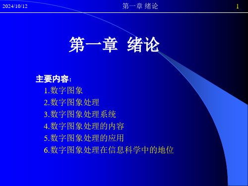
第一章绪论
17
2024/10/12
第一章绪论
18
2024/10/12
第一章绪论
19
2024/10/12
第一章绪论
20
<2>几何处理
放大、缩小、旋转，配准，几何校正，面积、周长计算。
请计算台湾的陆地面积
2024/10/12
第一章绪论
21
<3>图象复原
由图象的退化模型，求出原始图象
图像处理是指按照一定的目标，用一系列的操作来“改造”图像的方法.
2024/10/12
第一章绪论
7
➢图象处理技术的分类(从方法上进行分类)[2]
1．模拟图象处理（光学图像处理等）
用光学、电子等方法对模拟信号组成的图像，用光学器件、电子器件进行光学变换等处理得到所需结果（哈哈镜、望远镜，放大镜，电视等）.
2024/10/12
第一章绪论
22
<4>图象重建[3]
[3]此图像来自罗立民，脑成像，
2024/10/12
第一章绪论
23
/zhlshb/ct/lx.htm
2024/10/12
第一章绪论
图形用户界面，动画，网页制作等
2024/10/12象处理的基本概念，和基本问题，以及一些典型的应用。
2024/10/12
第一章绪论
33
提问
摄像头(机),扫描仪,CT成像装置,其他图象成像装置
2)图象的存储
各种图象存储压缩格式(JPEG,MPEG等),海量图象数据库技术
3)图象的传输
内部传输(DirectMemoryAccess),外部传输(主要是网络)

数字图像处理MATLAB程序大全1

数字图像处理MATLAB程序大全1%对一幅图像进行2倍、4倍、8倍和16倍减采样，显示结果。

a=imread('E:\lmt\ketangshiyan\ceshitu\Plane211.jpg');b=rgb2gray(a);for m=1:4figure[width,height]=size(b);quartimage=zeros(floor(width/(m)),floor(height/(2*m)));k=1;n=1;for i=1:(m):widthfor j=1:(2*m):heightquartimage(k,n)=b(i,j);n=n+1;endk=k+1;n=1;endimshow(uint8(quartimage));endI=imread('F:\work\Digital Image Processing\2015\ketangshiyan\ceshitu\Plane211.jpg');I2=rgb2gray(I);imshow(I);figure,imshow(I2);%读入源图像，BMP格式I=imread('F:\work\Digital Image Processing\2015\ketangshiyan\ceshitu\cameraman.bmp'); %显示图像I的基本信息whos I%显示图像imshow(I)%显示图像的详细信息，filename是存储在磁盘中的图像全名imfinfo('F:\work\Digital Image Processing\2015\ketangshiyan\ceshitu\cameraman.bmp') %保存图像I为jpg格式，压缩存储，q为图像质量，介于0-100之间的整数imwrite(I,'F:\work\Digital Image Processing\2015\ketangshiyan\ceshitu\cameraman1.jpg'); %以位图的格式存储图像imwrite(I,'F:\work\Digital Image Processing\2015\ketangshiyan\ceshitu\cameraman1.tif');%在同一个图像窗口显示多幅图像，并为每幅图像添加标题。

(完整版)数字图像处理代码大全

1.图像反转MATLAB程序实现如下：I=imread('xian.bmp');J=double(I);J=-J+(256-1); %图像反转线性变换H=uint8(J);subplot(1,2,1),imshow(I);subplot(1,2,2),imshow(H);2.灰度线性变换MATLAB程序实现如下：I=imread('xian.bmp');subplot(2,2,1),imshow(I);title('原始图像');axis([50,250,50,200]);axis on; %显示坐标系I1=rgb2gray(I);subplot(2,2,2),imshow(I1);title('灰度图像');axis([50,250,50,200]);axis on; %显示坐标系J=imadjust(I1,[0.1 0.5],[]); %局部拉伸，把[0.1 0.5]内的灰度拉伸为[0 1]subplot(2,2,3),imshow(J);title('线性变换图像[0.1 0.5]');axis([50,250,50,200]);grid on; %显示网格线axis on; %显示坐标系K=imadjust(I1,[0.3 0.7],[]); %局部拉伸，把[0.3 0.7]内的灰度拉伸为[0 1]subplot(2,2,4),imshow(K);title('线性变换图像[0.3 0.7]');axis([50,250,50,200]);grid on; %显示网格线axis on; %显示坐标系3.非线性变换MATLAB程序实现如下：I=imread('xian.bmp');I1=rgb2gray(I);subplot(1,2,1),imshow(I1);title('灰度图像');axis([50,250,50,200]);grid on; %显示网格线axis on; %显示坐标系J=double(I1);J=40*(log(J+1));H=uint8(J);subplot(1,2,2),imshow(H);title('对数变换图像');axis([50,250,50,200]);grid on; %显示网格线axis on; %显示坐标系4.直方图均衡化MATLAB程序实现如下：I=imread('xian.bmp');I=rgb2gray(I);figure;subplot(2,2,1);imshow(I);subplot(2,2,2);imhist(I);I1=histeq(I);figure;subplot(2,2,1);imshow(I1);subplot(2,2,2);imhist(I1);5.线性平滑滤波器用MATLAB实现领域平均法抑制噪声程序：I=imread('xian.bmp');subplot(231)imshow(I)title('原始图像')I=rgb2gray(I);I1=imnoise(I,'salt & pepper',0.02);subplot(232)imshow(I1)title('添加椒盐噪声的图像')k1=filter2(fspecial('average',3),I1)/255; %进行3*3模板平滑滤波k2=filter2(fspecial('average',5),I1)/255; %进行5*5模板平滑滤波k3=filter2(fspecial('average',7),I1)/255; %进行7*7模板平滑滤波k4=filter2(fspecial('average',9),I1)/255; %进行9*9模板平滑滤波subplot(233),imshow(k1);title('3*3模板平滑滤波');subplot(234),imshow(k2);title('5*5模板平滑滤波');subplot(235),imshow(k3);title('7*7模板平滑滤波');subplot(236),imshow(k4);title('9*9模板平滑滤波'); 6.中值滤波器用MATLAB实现中值滤波程序如下：I=imread('xian.bmp');I=rgb2gray(I);J=imnoise(I,'salt&pepper',0.02);subplot(231),imshow(I);title('原图像');subplot(232),imshow(J);title('添加椒盐噪声图像');k1=medfilt2(J); %进行3*3模板中值滤波k2=medfilt2(J,[5,5]); %进行5*5模板中值滤波k3=medfilt2(J,[7,7]); %进行7*7模板中值滤波k4=medfilt2(J,[9,9]); %进行9*9模板中值滤波subplot(233),imshow(k1);title('3*3模板中值滤波'); subplot(234),imshow(k2);title('5*5模板中值滤波'); subplot(235),imshow(k3);title('7*7模板中值滤波'); subplot(236),imshow(k4);title('9*9模板中值滤波'); 7.用Sobel算子和拉普拉斯对图像锐化：I=imread('xian.bmp');subplot(2,2,1),imshow(I);title('原始图像');axis([50,250,50,200]);grid on; %显示网格线axis on; %显示坐标系I1=im2bw(I);subplot(2,2,2),imshow(I1);title('二值图像');axis([50,250,50,200]);grid on; %显示网格线axis on; %显示坐标系H=fspecial('sobel'); %选择sobel算子J=filter2(H,I1); %卷积运算subplot(2,2,3),imshow(J);title('sobel算子锐化图像');axis([50,250,50,200]);grid on; %显示网格线axis on; %显示坐标系h=[0 1 0,1 -4 1,0 1 0]; %拉普拉斯算子J1=conv2(I1,h,'same'); %卷积运算subplot(2,2,4),imshow(J1);title('拉普拉斯算子锐化图像');axis([50,250,50,200]);grid on; %显示网格线axis on; %显示坐标系8.梯度算子检测边缘用MATLAB实现如下：I=imread('xian.bmp');subplot(2,3,1);imshow(I);title('原始图像');axis([50,250,50,200]);grid on; %显示网格线axis on; %显示坐标系I1=im2bw(I);subplot(2,3,2);imshow(I1);title('二值图像');axis([50,250,50,200]);grid on; %显示网格线axis on; %显示坐标系I2=edge(I1,'roberts');figure;subplot(2,3,3);imshow(I2);title('roberts算子分割结果');axis([50,250,50,200]);grid on; %显示网格线axis on; %显示坐标系I3=edge(I1,'sobel');subplot(2,3,4);imshow(I3);title('sobel算子分割结果');axis([50,250,50,200]);grid on; %显示网格线axis on; %显示坐标系I4=edge(I1,'Prewitt');subplot(2,3,5);imshow(I4);title('Prewitt算子分割结果');axis([50,250,50,200]);grid on; %显示网格线axis on; %显示坐标系9.LOG算子检测边缘用MATLAB程序实现如下：I=imread('xian.bmp');subplot(2,2,1);imshow(I);title('原始图像');I1=rgb2gray(I);subplot(2,2,2);imshow(I1);title('灰度图像');I2=edge(I1,'log');subplot(2,2,3);imshow(I2);title('log算子分割结果'); 10.Canny算子检测边缘用MATLAB程序实现如下：I=imread('xian.bmp'); subplot(2,2,1);imshow(I);title('原始图像')I1=rgb2gray(I);subplot(2,2,2);imshow(I1);title('灰度图像');I2=edge(I1,'canny'); subplot(2,2,3);imshow(I2);title('canny算子分割结果');11.边界跟踪（bwtraceboundary函数）clcclear allI=imread('xian.bmp');figureimshow(I);title('原始图像');I1=rgb2gray(I); %将彩色图像转化灰度图像threshold=graythresh(I1); %计算将灰度图像转化为二值图像所需的门限BW=im2bw(I1, threshold); %将灰度图像转化为二值图像figureimshow(BW);title('二值图像');dim=size(BW);col=round(dim(2)/2)-90; %计算起始点列坐标row=find(BW(:,col),1); %计算起始点行坐标connectivity=8;num_points=180;contour=bwtraceboundary(BW,[row,col],'N',connectivity,num_p oints);%提取边界figureimshow(I1);hold on;plot(contour(:,2),contour(:,1), 'g','LineWidth' ,2); title('边界跟踪图像');12.Hough变换I= imread('xian.bmp');rotI=rgb2gray(I);subplot(2,2,1);imshow(rotI);title('灰度图像');axis([50,250,50,200]);grid on;axis on;BW=edge(rotI,'prewitt');subplot(2,2,2);imshow(BW);title('prewitt算子边缘检测后图像');axis([50,250,50,200]);grid on;axis on;[H,T,R]=hough(BW);subplot(2,2,3);imshow(H,[],'XData',T,'YData',R,'InitialMagnification','fit'); title('霍夫变换图');xlabel('\theta'),ylabel('\rho');axis on , axis normal, hold on;P=houghpeaks(H,5,'threshold',ceil(0.3*max(H(:))));x=T(P(:,2));y=R(P(:,1));plot(x,y,'s','color','white');lines=houghlines(BW,T,R,P,'FillGap',5,'MinLength',7); subplot(2,2,4);,imshow(rotI);title('霍夫变换图像检测');axis([50,250,50,200]);grid on;axis on;hold on;max_len=0;for k=1:length(lines)xy=[lines(k).point1;lines(k).point2];plot(xy(:,1),xy(:,2),'LineWidth',2,'Color','green');plot(xy(1,1),xy(1,2),'x','LineWidth',2,'Color','yellow');plot(xy(2,1),xy(2,2),'x','LineWidth',2,'Color','red');len=norm(lines(k).point1-lines(k).point2);if(len>max_len)max_len=len;xy_long=xy;endendplot(xy_long(:,1),xy_long(:,2),'LineWidth',2,'Color','cyan'); 13.直方图阈值法用MATLAB实现直方图阈值法：I=imread('xian.bmp');I1=rgb2gray(I);figure;subplot(2,2,1);imshow(I1);title('灰度图像')axis([50,250,50,200]);grid on; %显示网格线axis on; %显示坐标系[m,n]=size(I1); %测量图像尺寸参数GP=zeros(1,256); %预创建存放灰度出现概率的向量for k=0:255GP(k+1)=length(find(I1==k))/(m*n); %计算每级灰度出现的概率，将其存入GP中相应位置endsubplot(2,2,2),bar(0:255,GP,'g') %绘制直方图title('灰度直方图')xlabel('灰度值')ylabel('出现概率')I2=im2bw(I,150/255);subplot(2,2,3),imshow(I2);title('阈值150的分割图像')axis([50,250,50,200]);grid on; %显示网格线axis on; %显示坐标系I3=im2bw(I,200/255); %subplot(2,2,4),imshow(I3);title('阈值200的分割图像')axis([50,250,50,200]);grid on; %显示网格线axis on; %显示坐标系14. 自动阈值法：Otsu法用MATLAB实现Otsu算法：clcclear allI=imread('xian.bmp');subplot(1,2,1),imshow(I);title('原始图像')axis([50,250,50,200]);grid on; %显示网格线axis on; %显示坐标系level=graythresh(I); %确定灰度阈值BW=im2bw(I,level);subplot(1,2,2),imshow(BW);title('Otsu法阈值分割图像')axis([50,250,50,200]);grid on; %显示网格线axis on; %显示坐标系15.膨胀操作I=imread('xian.bmp'); %载入图像I1=rgb2gray(I);subplot(1,2,1);imshow(I1);title('灰度图像')axis([50,250,50,200]);grid on; %显示网格线axis on; %显示坐标系se=strel('disk',1); %生成圆形结构元素I2=imdilate(I1,se); %用生成的结构元素对图像进行膨胀subplot(1,2,2);imshow(I2);title('膨胀后图像');axis([50,250,50,200]);grid on; %显示网格线axis on; %显示坐标系16.腐蚀操作MATLAB实现腐蚀操作I=imread('xian.bmp'); %载入图像I1=rgb2gray(I);subplot(1,2,1);imshow(I1);title('灰度图像')axis([50,250,50,200]);grid on; %显示网格线axis on; %显示坐标系se=strel('disk',1); %生成圆形结构元素I2=imerode(I1,se); %用生成的结构元素对图像进行腐蚀subplot(1,2,2);imshow(I2);title('腐蚀后图像');axis([50,250,50,200]);grid on; %显示网格线axis on; %显示坐标系17.开启和闭合操作用MATLAB实现开启和闭合操作I=imread('xian.bmp'); %载入图像subplot(2,2,1),imshow(I);title('原始图像');axis([50,250,50,200]);axis on; %显示坐标系I1=rgb2gray(I);subplot(2,2,2),imshow(I1);title('灰度图像');axis([50,250,50,200]);axis on; %显示坐标系se=strel('disk',1); %采用半径为1的圆作为结构元素I3=imclose(I1,se); %闭合操作subplot(2,2,3),imshow(I2);title('开启运算后图像');axis([50,250,50,200]);axis on; %显示坐标系subplot(2,2,4),imshow(I3);title('闭合运算后图像');axis([50,250,50,200]);axis on; %显示坐标系18.开启和闭合组合操作I=imread('xian.bmp'); %载入图像subplot(3,2,1),imshow(I);title('原始图像');axis([50,250,50,200]);axis on; %显示坐标系I1=rgb2gray(I);subplot(3,2,2),imshow(I1);title('灰度图像');axis([50,250,50,200]);axis on; %显示坐标系se=strel('disk',1);I3=imclose(I1,se); %闭合操作subplot(3,2,3),imshow(I2);title('开启运算后图像');axis([50,250,50,200]);axis on; %显示坐标系subplot(3,2,4),imshow(I3);title('闭合运算后图像');axis([50,250,50,200]);axis on; %显示坐标系se=strel('disk',1);I4=imopen(I1,se);I5=imclose(I4,se);subplot(3,2,5),imshow(I5); %开—闭运算图像title('开—闭运算图像');axis([50,250,50,200]);axis on; %显示坐标系I6=imclose(I1,se);I7=imopen(I6,se);subplot(3,2,6),imshow(I7); %闭—开运算图像title('闭—开运算图像');axis([50,250,50,200]);axis on; %显示坐标系19.形态学边界提取利用MATLAB实现如下：I=imread('xian.bmp'); %载入图像subplot(1,3,1),imshow(I);title('原始图像');axis([50,250,50,200]);grid on; %显示网格线axis on; %显示坐标系I1=im2bw(I);subplot(1,3,2),imshow(I1);title('二值化图像');axis([50,250,50,200]);grid on; %显示网格线axis on; %显示坐标系I2=bwperim(I1); %获取区域的周长subplot(1,3,3),imshow(I2);title('边界周长的二值图像');axis([50,250,50,200]);grid on;axis on;20.形态学骨架提取利用MATLAB实现如下：I=imread('xian.bmp'); subplot(2,2,1),imshow(I); title('原始图像');axis([50,250,50,200]); axis on;I1=im2bw(I);subplot(2,2,2),imshow(I1); title('二值图像');axis([50,250,50,200]); axis on;I2=bwmorph(I1,'skel',1); subplot(2,2,3),imshow(I2); title('1次骨架提取');axis([50,250,50,200]); axis on;I3=bwmorph(I1,'skel',2); subplot(2,2,4),imshow(I3); title('2次骨架提取');axis([50,250,50,200]); axis on;21.直接提取四个顶点坐标I = imread('xian.bmp');I = I(:,:,1);BW=im2bw(I);figureimshow(~BW)[x,y]=getpts。

数字图像处理matlab代码

一、编写程序完成不同滤波器的图像频域降噪和边缘增强的算法并进行比较，得出结论。

1、不同滤波器的频域降噪1.1 理想低通滤波器(ILPF)和二阶巴特沃斯低通滤波器(BLPF)clc;clear all;close all;I1=imread('me.jpg');I1=rgb2gray(I1);subplot(2,2,1),imshow(I1),title('原始图像');I2=imnoise(I1,'salt & pepper');subplot(2,2,2),imshow(I2),title('噪声图像');F=double(I2);g = fft2(F);g = fftshift(g);[M, N]=size(g);result1=zeros(M,N);result2=zeros(M,N);nn = 2;d0 =50;m = fix(M/2);n = fix(N/2);for i = 1:Mfor j = 2:Nd = sqrt((i-m)^2+(j-n)^2);h = 1/(1+0.414*(d/d0)^(2*nn));result1(i,j) = h*g(i,j);if(g(i,j)< 50)result2(i,j) = 0;elseresult2(i,j) =g(i,j);endendendresult1 = ifftshift(result1);result2 = ifftshift(result2);J2 = ifft2(result1);J3 = uint8(real(J2));subplot(2, 2, 3),imshow(J3,[]),title('巴特沃斯低通滤波结果'); J4 = ifft2(result2);J5 = uint8(real(J4));subplot(2, 2, 4),imshow(J5,[]),title('理想低通滤波结果');实验结果：原始图像噪声图像巴特沃斯低通滤波结果理想低通滤波结果1.2 指数型低通滤波器(ELPF)clc;clear all;close all;I1=imread('me.jpg');I1=rgb2gray(I1);I2=im2double(I1);I3=imnoise(I2,'gaussian',0.01);I4=imnoise(I3,'salt & pepper',0.01);subplot(1,3,1),imshow(I2), title('原始图像'); %显示原始图像subplot(1,3,2),imshow(I4),title('加入混合躁声后图像 ');s=fftshift(fft2(I4));%将灰度图像的二维不连续Fourier 变换的零频率成分移到频谱的中心[M,N]=size(s); %分别返回s的行数到M中，列数到N中n1=floor(M/2); %对M/2进行取整n2=floor(N/2); %对N/2进行取整d0=40;for i=1:Mfor j=1:Nd=sqrt((i-n1)^2+(j-n2)^2); %点（i,j）到傅立叶变换中心的距离 h=exp(log(1/sqrt(2))*(d/d0)^2);s(i,j)=h*s(i,j); %ILPF滤波后的频域表示endends=ifftshift(s); %对s进行反FFT移动s=im2uint8(real(ifft2(s)));subplot(1,3,3),imshow(s),title('ELPF滤波后的图像（d=40）');运行结果：1.3 梯形低通滤波器(TLPF)clc;clear all;close all;I1=imread('me.jpg');I1=rgb2gray(I1); %读取图像I2=im2double(I1);I3=imnoise(I2,'gaussian',0.01);I4=imnoise(I3,'salt & pepper',0.01);subplot(1,3,1),imshow(I2),title('原始图像'); %显示原始图像subplot(1,3,2),imshow(I4),title('加噪后的图像');s=fftshift(fft2(I4));%将灰度图像的二维不连续Fourier 变换的零频率成分移到频谱的中心[M,N]=size(s); %分别返回s的行数到M中，列数到N中n1=floor(M/2); %对M/2进行取整n2=floor(N/2); %对N/2进行取整d0=10;d1=160;for i=1:Mfor j=1:Nd=sqrt((i-n1)^2+(j-n2)^2); %点（i,j）到傅立叶变换中心的距离 if (d<=d0)h=1;else if (d0<=d1)h=(d-d1)/(d0-d1);else h=0;endends(i,j)=h*s(i,j); %ILPF滤波后的频域表示endends=ifftshift(s); %对s进行反FFT移动s=im2uint8(real(ifft2(s))); %对s进行二维反离散的Fourier变换后，取复数的实部转化为无符号8位整数subplot(1,3,3),imshow(s),title('TLPF滤波后的图像');运行结果：1.4 高斯低通滤波器(GLPF)clear all;clc;close all;I1=imread('me.jpg');I1=rgb2gray(I1);I2=im2double(I1);I3=imnoise(I2,'gaussian',0.01);I4=imnoise(I3,'salt & pepper',0.01);subplot(1,3,1),imshow(I2),title('原始图像');subplot(1,3,2),imshow(I4),title('加噪后的图像');s=fftshift(fft2(I4));%将灰度图像的二维不连续Fourier 变换的零频率成分移到频谱的中心[M,N]=size(s); %分别返回s的行数到M中，列数到N中n1=floor(M/2); %对M/2进行取整n2=floor(N/2); %对N/2进行取整d0=40;for i=1:Mfor j=1:Nd=sqrt((i-n1)^2+(j-n2)^2); %点（i,j）到傅立叶变换中心的距离 h=1*exp(-1/2*(d^2/d0^2)); %GLPF滤波函数s(i,j)=h*s(i,j); %ILPF滤波后的频域表示endends=ifftshift(s); %对s进行反FFT移动s=im2uint8(real(ifft2(s))); %对s进行二维反离散的Fourier变换后，取复数的实部转化为无符号8位整数subplot(1,3,3),imshow(s),title('GLPF滤波后的图像（d=40）');运行结果：1.5 维纳滤波器clc;clear all;close all;I=imread('me.jpg'); %读取图像I=rgb2gray(I);I1=im2double(I);I2=imnoise(I1,'gaussian',0.01);I3=imnoise(I2,'salt & pepper',0.01);I4=wiener2(I3);subplot(1,3,1),imshow(I1),title('原始图像'); %显示原始图像subplot(1,3,2),imshow(I3),title('加入混合躁声后图像');I4=wiener2(I3);subplot(1,3,3),imshow(I4),title('wiener滤波后的图像');运行结果：结论：理想低通滤波器，虽然有陡峭的截止频率，却不能产生良好的效果，图像由于高频分量的滤除而变得模糊，同时还产生振铃效应。

(完整版)MATLAB在数字图像处理中的应用正文毕业设计

以下文档格式全部为word格式，下载后您可以任意修改编辑。

目录1 绪论 (1)1.1 研究背景 (1)1.2 课题研究目的和意义 (2)1.3研究内容 (2)2 数字图像处理的基础知识简介 (2)2.1 什么是数字图像 (2)2.2 数字图像处理概述 (4)2.2.1 基本概念 (4)2.2.2 研究内容 (4)2.2.3 基本特点 (6)2.2.4 主要应用 (6)2.3 图像处理文件格式 (7)2.3.1 MATLAB图像文件格式 (7)2.3.2 图像类型 (8)3 利用MATLAB增强图像清晰度 (9)3.1 空域变换增强 (9)3.1.1 增强对比度 (9)3.1.2 图像求反 (11)3.2 空域滤波增强 (12)3.2.1 基本原理 (12)3.2.2 线性平滑滤波器 (13)3.2.3 非线性平滑滤波器 (14)3.2.4 线性锐化滤波器 (15)3.3 频域增强 (16)3.3.1 基本原理 (16)3.3.2 低通滤波 (17)3.3.3 高通滤波 (18)4 结束语 (20)参考文献 (21)致谢 (22)1 绪论1.1 研究背景数字图像处理最早出现于20世纪50年代，当时的电子计算机已经发展到一定水平，人们开始利用计算机来处理图形和图像信息。

数字图像处理作为一门学科大约形成于20世纪60年代初期。

早期的图像处理的目的是改善图像的质量，它以人为对象，以改善人的视觉效果为目的。

图像处理中，输入的是质量低的图像，输出的是改善质量后的图像，常用的图像处理方法有图像增强、复原、编码、压缩等。

首次获得实际成功应用的是美国喷气推进实验室(JPL)。

他们对航天探测器徘徊者7号在1964年发回的几千张月球照片使用了图像处理技术，如几何校正、灰度变换、去除噪声等方法进行处理，并考虑了太阳位置和月球环境的影响，由计算机成功地绘制出月球表面地图，获得了巨大的成功。

随后又对探测飞船发回的近十万张照片进行更为复杂的图像处理，以致获得了月球的地形图、彩色图及全景镶嵌图，为人类登月创举奠定了坚实的基础，也推动了数字图像处理这门学科的诞生。

非常全非常详细的MATLAB数字图像处理技术

MATLAB数字图像处理1 概述BW=dither(I)灰度转成二值图；X=dither(RGB,map)RGB转成灰度图，用户需要提供一个Colormap；[X,map]=gray2ind(I,n)灰度到索引；[X,map]=gray2ind(BW,n)二值图到索引，map可由gray(n)产生。

灰度图n默认64，二值图默认2；X=graylice(I,n)灰度图到索引图，门限1/n,2/n,…,(n-1)/n，X=graylice(I,v)给定门限向量v；BW=im2bw(I,level)灰度图I到二值图；BW=im2bw(X,map,level)索引图X到二值图；level是阈值门限，超过像素为1，其余置0，level在[0,1]之间。

BW=im2bw(RGB,level)RGB到二值图；I=ind2gray(X,map)索引图到灰度图；RGB=ind2rgb(X,map)索引图到RGB；I=rgb2gray(RGB)RGB到灰度图。

2 图像运算2.1 图像的读写MATLAB支持的图像格式有bmp,gif,ico,jpg,png,cur，pcx,xwd和tif。

读取（imread）：[1] A=imread(filename,fmt)[2] [X,map]=imread(filename,fmt)[3] […]=imread(filename)[4] […]=imread(URL,…)说明：filename是图像文件名，如果不在搜索路径下应是图像的全路径，fmt是图像文件扩展名字符串。

前者可读入二值图、灰度图、彩图(主要是RGB)；第二个读入索引图，map 为索引图对应的Colormap,即其相关联的颜色映射表，若不是索引图则map为空。

URL表示引自Internet URL中的图像。

写入（imwrite）：[1] R=imwrite(A,filename,fmt);[2] R=imwrite(X,map,filename,fmt);[3] R=imwrite(…,filename);[4] R=imwrite(…,Param1,V al1,Param2,Val2)说明：针对第四个，该语句用于指定HDF,JPEG,PBM,PGM,PNG,PPM,TIFF等类型输出文件的不同参数。

数字图像处理基础程序及运行结果图像matlab程序

目录实验一MATLAB数字图像处理初步 (2)实验二图像的代数运算 (7)实验三图像增强—灰度变换 (11)实验四图像增强—直方图变换 (14)实验五图像增强—空域滤波 (16)实验六图像的傅立叶变换 (22)实验七图像增强—频域滤波 (24)实验八彩色图像处理 (27)实验九图像分割 (33)实验十形态学运算 (36)实验一 MATLAB数字图像处理初步一、实验目的与要求1．熟悉及掌握在MATLAB中能够处理哪些格式图像。

2．熟练掌握在MATLAB中如何读取图像。

3．掌握如何利用MATLAB来获取图像的大小、颜色、高度、宽度等等相关信息。

4．掌握如何在MATLAB中按照指定要求存储一幅图像的方法。

5．图像间如何转化。

二、实验内容及步骤1．利用imread( )函数读取一幅图像，假设其名为flower.tif，存入一个数组中；2．利用whos 命令提取该读入图像flower.tif的基本信息；3．利用imshow()函数来显示这幅图像；4．利用imfinfo函数来获取图像文件的压缩，颜色等等其他的详细信息；5．利用imwrite()函数来压缩这幅图象，将其保存为一幅压缩了像素的jpg 文件,设为flower.jpg；语法：imwrite(原图像，新图像，‘quality’,q), q取0-100。

6．同样利用imwrite()函数将最初读入的tif图象另存为一幅bmp图像，设为flower.bmp。

7．用imread()读入图像：Lenna.jpg 和camema.jpg；8．用imfinfo()获取图像Lenna.jpg和camema.jpg 的大小；9．用figure,imshow()分别将Lenna.jpg和camema.jpg显示出来，观察两幅图像的质量。

10．用im2bw将一幅灰度图像转化为二值图像，并且用imshow显示出来观察图像的特征。

11．将每一步的函数执行语句拷贝下来，写入实验报告，并且将得到第3、9、10步得到的图像效果拷贝下来三、考核要点1、熟悉在MATLAB中如何读入图像、如何获取图像文件的相关信息、如何显示图像及保存图像等，熟悉相关的处理函数。

数字图像处理：图像的灰度变换（Matlab实现）

数字图像处理：图像的灰度变换（Matlab实现）(1)线性变换:通过建⽴灰度映射来调整源图像的灰度。

k>1增强图像的对⽐度；k=1调节图像亮度，通过改变d值达到调节亮度⽬的；0i = imread('theatre.jpg');i = im2double(rgb2gray(i));[m,n]=size(i);%增加对⽐度Fa = 1.25; Fb = 0;O = Fa.*i + Fb/255;figure(1), subplot(221), imshow(O);title('Fa = 1.25, Fb = 0, contrast increasing');figure(2),subplot(221), [H,x]=imhist(O, 64);stem(x, (H/m/n), '.');title('Fa = 1.25, Fb = 0, contrast increasing');%减⼩对⽐度Fa =0.5; Fb = 0;O = Fa.*i + Fb/255;figure(1), subplot(222),imshow(O);title('Fa = 0.5, Fb = 0, contrast decreasing');figure(2), subplot(222), [H,x] = imhist(O, 64);stem(x, (H/m/n), '.');title('Fa = 0.5, Fb = 0, contrast decreasing');%线性亮度增加Fa = 0.5; Fb = 50;O = Fa.*i + Fb/255;figure(1), subplot(223), imshow(O);title('Fa = 0.5, Fb = 50, brightness control');figure(2), subplot(223), [H,x]=imhist(O,64);stem(x, (H/m/n), '.');title('Fa = 0.5, Fb = 50, brightness control');%反相显⽰Fa = -1; Fb = 255;O = Fa.*i + Fb/255;figure(1), subplot(224), imshow(O);title('Fa = -1, Fb = 255, reversal processing');figure(2), subplot(224),[H,x]=imhist(O, 64);stem(x, (H/m/n), '.');title('Fa = -1, Fb = 255, reversal processing');(2)对数变换：增强低灰度，减弱⾼灰度值。

MATLAB图像处理(实例+代码)

MATLAB图像处理(1) %%%%%%%%%%%%%%%%%%%%%%%%%%%%%%%%%%%%%%%%%%%%%%%%%%%%%%%%%% %测量交角(线性拟合的思想）%Step 1: Load image%Step 2: Extract the region of interest%Step 3: Threshold the image%Step 4: Find initial point on each boundary%Step 5: Trace the boundaries%Step 6: Fit lines to the boundaries%Step 7: Find the angle of intersection%Step 8: Find the point of intersection%Step 9: Plot the results.clc;clear;close all;%Step 1: Load imageRGB = imread('gantrycrane.png');imshow(RGB);%Step 2: Extract the region of interest% pixel information displayed by imviewstart_row = 34;start_col = 208;cropRGB = RGB(start_row:163, start_col:400, :);figure, imshow(cropRGB)% Store (X,Y) offsets for later use; subtract 1 so that each offset will% correspond to the last pixel before the region of interestoffsetX = start_col-1;offsetY = start_row-1;%Step 3: Threshold the imageI = rgb2gray(cropRGB);threshold = graythresh(I);BW = im2bw(I,threshold);BW = ~BW; % complement the image (objects of interest must be white) figure, imshow(BW)%Step 4: Find initial point on each boundarydim = size(BW);% horizontal beamcol1 = 4;row1 = min(find(BW(:,col1)));% angled beamrow2 = 12;col2 = min(find(BW(row2,:)));%Step 5: Trace the boundariesboundary1 = bwtraceboundary(BW, [row1, col1], 'N', 8, 70);% set the search direction to counterclockwise, in order to trace downward. boundary2 = bwtraceboundary(BW, [row2, col2], 'E', 8, 90,'counter'); figure, imshow(RGB); hold on;% apply offsets in order to draw in the original imageplot(offsetX+boundary1(:,2),offsetY+boundary1(:,1),'g','LineWidth',2); plot(offsetX+boundary2(:,2),offsetY+boundary2(:,1),'g','LineWidth',2);%Step 6: Fit lines to the boundariesab1 = polyfit(boundary1(:,2), boundary1(:,1), 1);ab2 = polyfit(boundary2(:,2), boundary2(:,1), 1);%Step 7: Find the angle of intersectionvect1 = [1 ab1(1)]; % create a vector based on the line equationvect2 = [1 ab2(1)];dp = dot(vect1, vect2);% compute vector lengthslength1 = sqrt(sum(vect1.^2));length2 = sqrt(sum(vect2.^2));% obtain the larger angle of intersection in degreesangle = 180-acos(dp/(length1*length2))*180/pi%Step 8: Find the point of intersectionintersection = [1 ,-ab1(1); 1, -ab2(1)] \ [ab1(2); ab2(2)];% apply offsets in order to compute the location in the original,% i.e. not cropped, image.intersection = intersection + [offsetY; offsetX]%Step 9: Plot the results.inter_x = intersection(2);inter_y = intersection(1);% draw an "X" at the point of intersectionplot(inter_x,inter_y,'yx','LineWidth',2);text(inter_x-60, inter_y-30, [sprintf('%1.3f',angle),'{\circ}'],...'Color','y','FontSize',14,'FontWeight','bold');interString = sprintf('(%2.1f,%2.1f)', inter_x, inter_y);text(inter_x-10, inter_y+20, interString,...'Color','y','FontSize',14,'FontWeight','bold');%%%%%%%%%%%%%%%%%%%%%%%%%%%%%%%%%%%%%%%%%%%%%%%%%%%%%%% %%%%检测一段圆弧的半径（圆形拟合）%Step 1: Read image%Step 2: Threshold the image%Step 3: Extract initial boundary point location%Step 4: Trace the boundaries%Step 5: Fit a circle to the boundary %%%%%%%%%%%%%%%%%%%%%%%%%%%%%%%%%%%%%%%%%%%%%%%%%%%%%%% %%%%2006.6.23基于特征的与运算>> load imdemos dots box>> imshow(dots)>> figure,imshow(box)>> logical_and=box&dots;>> imshow(logical_and);>> [r,c]=find(logical_and);>> feature_and=bwselect(dots,c,r);>> figure,imshow(feature_and); %%%%%%%%%%%%%%%%%%%%%%%%%%%%%%%%%%%%%%%%%%%%%%%%%%%%%%% %%%%利用逻辑运算，提取含有细胞核的细胞load imdemos bacteria;imshow(bacteria);bact_bw=(bacteria>=100);%figure,imshow(bact_bw);bact_bw=~bact_bw;figure,imshow(bact_bw); %直接二值取反figure,imshow(bact_bw)%细胞和细胞核重叠在一起，无法区分%进行Laplace算子滤波，突出核与胞的区别filtered=filter2(fspecial('laplacian'),bacteria);>> figure,imshow(filtered) %先拉氏滤波>> bact_granules=(filtered>-4);figure,imshow(bact_granules); %“－4”运算bact_granules=bact_granules&bact_bw; %特征与运算figure,imshow(bact_granules);erode_bw=erode(bact_bw); %%figure,imshow(erode_bw);nobord=imclearborder(erode_bw); %fill_bw=imfill(nobord,'holes');figure,imshow(fill_bw);%fill_bw=bwfill(erode_bw,'holes');%figure,imshow(fill_bw);bact_granules_0=(bact_granules==0); %判0运算的结果,等价与figure,imshow(bact_granules_0); %下边的取反运算！%bact_granules_anti=~bact_granules;%figure,imshow(bact_granules_anti);>> granules=fill_bw&bact_granules_0; %尽可能多地把“核”提取出来>> figure,imshow(granules)>> [r,c]=find(granules);>> result=bwselect(bact_bw,c,r);>> figure,imshow(bacteria);>> figure,imshow(result) %%%%%%%%%%%%%%%%%%%%%%%%%%%%%%%%%%%%%%%%%%%%%%%%%%%%%%% %%%%2006.7.15%按顺序标记每一个连通区域clc;clear;close all;%Step 1: Read image%Step 2: Threshold the image%Step 3: Remove the noise%Step 4: Find the boundaries%Step 5: Determine which objects are round>> RGB = imread('pillsetc.png');>> imshow(RGB)>> I = rgb2gray(RGB);>> threshold = graythresh(I);>> bw = im2bw(I,threshold);>> bw = bwareaopen(bw,30);>> se = strel('disk',2);>> bw = imclose(bw,se);>> bw = imfill(bw,'holes');>> [B,L] = bwboundaries(bw,'noholes');>> figure,imshow(label2rgb(L, @jet, [.5 .5 .5]))>> hold on>> data=regionprops(L,'all');>> centr=[data.Centroid]; %标记在重心上>> nums=1:length(B); %需要标记的物体个数for k = 1:length(B)boundary = B{k};plot(boundary(:,2), boundary(:,1), 'w', 'LineWidth', 2)signal=num2str(nums(k));text(centr(2*k-1),centr(2*k),signal) %按序标记物体endfor k=1:length(B) %画出每个区域的最小凸边形plot(data(k).ConvexHull(:,1),data(k).ConvexHull(:,2),'b','LineWidth',2) end>> stats = regionprops(L,'Area','Centroid');>> stats = regionprops(L,'Area','Centroid');threshold = 0.94;for k = 1:length(B)boundary = B{k};delta_sq = diff(boundary).^2;perimeter = sum(sqrt(sum(delta_sq,2)));area = stats(k).Area;metric = 4*pi*area/perimeter^2;metric_string = sprintf('%2.2f',metric);if metric > thresholdcentroid = stats(k).Centroid;plot(centroid(1),centroid(2),'ko');endtext(boundary(1,2)-35,boundary(1,1)+13,metric_string,'Color','y',...'FontSize',14,'FontWeight','bold');end>> title(['Metrics closer to 1 indicate that ',...'the object is approximately round']);%%%%%%%%%%%%%%%%%%%%%%%%%%%%%%%%%%%%%%%%%%%%%%%%%%%%%%% %%%%%%%%%%%%%%%2006.7.17%果穗梗、花椒籽分离%d:\matlab7\toolbox\images\images\truesize.m*(308行)clear;close all;clc>> i=imread('huaj_600_rgb.tif');>> figure,imshow(i);>> ig=rgb2gray(i);>> imed=medfilt2(ig);>> imedcanny=edge(imed,'canny');>> se90=strel('line',2,90);se0=strel('line',2,0);bwsdil=imdilate(imedcanny,[se90 se0]);%>> figure,imshow(bwsdil)>> ifill=imfill(bwsdil,'holes');>> bwero=imerode(ifill,[se90 se0]);>> nosmall=bwareaopen(bwero,3000,4);>> nobord=imclearborder(nosmall,4);figure,imshow(nobord);>> [labeled,numobjects]=bwlabel(nobord,4);rgb_label=label2rgb(labeled,@spring,'c','shuffle');figure,imshow(rgb_label);mexdata=regionprops(labeled,'all');hold on;centr=[mexdata.Centroid]; %寻找重心位置nums=1:numobjects;for k = 1:numobjectssoli=mexdata(k).Solidity;soli_string=sprintf('%2.2f',soli); %等价于转字符串% signal=num2str(nums(k));signal=sprintf('%d',k); %直接使用打印语句打印序号text(centr(2*k-1),centr(2*k),signal) %按序标记物体text(centr(2*k-1)-30,centr(2*k)-30,soli_string) %标注每个Solidity值end%画最小凸多边形>> for k=1:numobjectsplot(mexdata(k).ConvexHull(:,1),mexdata(k).ConvexHull(:,2),...'b','Linewidth',2)endhold off;%作出Solidity值的分布图，以之选定阈值>> figure,hist([mexdata.Solidity],255)%只显示Solidity>0.92的物体的图像>> idx = find([mexdata.Solidity] > 0.95);>> nut = ismember(labeled,idx);>> figure,imshow(nut)>> [labnut,numnut]=bwlabel(nut,4);>> numnut %数出花椒籽的粒数>> %只显示Solidity<0.92的物体的图像idx = find([mexdata.Solidity] < 0.75);peduncle = ismember(labeled,idx);figure,imshow(peduncle)>> [labped,numped]=bwlabel(peduncle,4);>> numped %数出含果穗梗的花椒数>> %只显示无果穗梗的花椒图像idx = find([mexdata.Solidity]>=0.75&[mexdata.Solidity]<=0.95);pure = ismember(labeled,idx);figure,imshow(pure)>> [labpure,numpure]=bwlabel(pure,4);>> numpure %纯净花椒的粒数%分别对籽，皮，梗使用regionprops函数>> nutdata=regionprops(labnut,'all');>> peddata=regionprops(labped,'all');>> puredata=regionprops(labpure,'all'); %%%%%%%%%%%%%%%%%%%%%%%%%%%%%%%%%%%%%%%%%%%%%%%%%%%%%%% %%%%%%%%%%%%%%%封装成一个函数function huaj();%对花椒图像进行处理imname=input('input an image name:','s');i=imread(imname);figure,imshow(i);ig=rgb2gray(i);imed=medfilt2(ig);imedcanny=edge(imed,'canny');se90=strel('line',2,90);se0=strel('line',2,0);bwsdil=imdilate(imedcanny,[se90 se0]);%figure,imshow(bwsdil)ifill=imfill(bwsdil,'holes');bwero=imerode(ifill,[se90 se0]);nosmall=bwareaopen(bwero,3000,4);nobord=imclearborder(nosmall,4);figure,imshow(nobord);[labeled,numobjects]=bwlabel(nobord,4);rgb_label=label2rgb(labeled,@spring,'c','shuffle');figure,imshow(rgb_label);mexdata=regionprops(labeled,'all');hold on;centr=[mexdata.Centroid]; %寻找重心位置nums=1:numobjects;for k = 1:numobjectssoli=mexdata(k).Solidity;soli_string=sprintf('%2.2f',soli); %等价于转字符串% signal=num2str(nums(k));signal=sprintf('%d',k); %直接使用打印语句打印序号text(centr(2*k-1),centr(2*k),signal) %按序标记物体text(centr(2*k-1)-30,centr(2*k)-30,soli_string) %标注每个Solidity值end%画最小凸多边形for k=1:numobjectsplot(mexdata(k).ConvexHull(:,1),mexdata(k).ConvexHull(:,2),...'b','Linewidth',2)endhold off;%作出Solidity值的分布图，以之选定阈值figure,hist([mexdata.Solidity],255)%只显示Solidity>0.92的物体的图像idx = find([mexdata.Solidity] > 0.92);nut = ismember(labeled,idx);figure,imshow(nut)[labnut,numnut]=bwlabel(nut,4);numnut %数出花椒籽的粒数%只显示Solidity<0.75的果穗梗图像idx = find([mexdata.Solidity] < 0.75);peduncle = ismember(labeled,idx);figure,imshow(peduncle)[labped,numped]=bwlabel(peduncle,4);numped %数出含果穗梗的花椒数%只显示无果穗梗的花椒果皮图像idx = find([mexdata.Solidity]>=0.75&[mexdata.Solidity]<=0.92);pure = ismember(labeled,idx);figure,imshow(pure)[labpure,numpure]=bwlabel(pure,4);numpure %纯净花椒的粒数%分别对籽，皮，梗使用regionprops函数nutdata=regionprops(labnut,'all');peddata=regionprops(labped,'all');puredata=regionprops(labpure,'all');%封装成一个函数%%%%%%%%%%%%%%%%%%%%%%%%%%%%%%%%%%%%%%%%%%%%%%%%%%%%%%% %%%%%%%%%%%%%%%%%%%%%%%%%%%%%%%%%%%%%%%%%%%%%%%%%%%%%%%%%%%%%%%%%%%%% %%%%%%%%%%%%%%%2006.7.18%命令文件%rice_1.m>> i=imread('rice.png');>> imshow(i);>> background=imopen(i,strel('disk',15));>> i2=imsubtract(i,background);>> figure,imshow(i2);>> i3=imadjust(i2,stretchlim(i2),[0 1]);>> figure,imshow(i3);>> level=graythresh(i3);>> bw=im2bw(i3,level);>> figure,imshow(bw);>> [labeled,numobjects]=bwlabel(bw,4);%函数文件%rice.mfunction y=rice;str=input('enter a image name:','s');i=imread(str);imshow(i);background=imopen(i,strel('disk',15));i2=imsubtract(i,background);figure,imshow(i2);i3=imadjust(i2,stretchlim(i2),[0 1]);figure,imshow(i3);level=graythresh(i3);bw=im2bw(i3,level);figure,imshow(bw);[labeled,numobjects]=bwlabel(bw,4);label_rgb=label2rgb(labeled,@spring,'c','shuffle');y=label_rgb; %%%%%%%%%%%%%%%%%%%%%%%%%%%%%%%%%%%%%%%%%%%%%%%%%%%%%%% %%%%%%%%%%%%%%%用if-else-end结构来控制循环，使之跳出或中断for或while循环a(1)=1;a(2)=2;for i=2:50a(i+1)=a(i-1)+a(i);i=i+1;if a(i)>10000 %查找第一个大于10000的元素break %用if语句控制for循环endendi,a(i)%用递归调用形式计算n!%(1)编写递归调用函数文件factor.mfunction f=factor(n);%factor.m 计算n!if n==1f=1;return;elsef=n*factor(n-1);return;end%(2)运行函数文件factor(6)%函数参数传递function sa=circle(r,s);%CIRCLE PLOT A CIRCLE OF RADIUS R IN THE LINE SPECIFIED BY S. %r%s%sa%%circle(r)%circle(r,s)%sa=circle(r)%sa=circle(r,s)if nargin==1%若输入参数数目为1，则该输入参数是指定的半径数值，%默认的圆周线颜色是蓝色s='b';end;clf;t=0:pi/100:2*pi;x=r*exp(i*t);if nargout==0plot(x,s);elsesa=pi*r*r;fill(real(x),imag(x),s)endaxis('square')。

使用MATLAB进行图像处理的步骤

使用MATLAB进行图像处理的步骤引言图像处理是一门研究如何对图像进行数字化处理和分析的技术，它在日常生活中得到了广泛的应用。

MATLAB作为一种强大的数学计算软件，具有丰富的图像处理功能，可以帮助用户快速、准确地处理图像数据。

本文将介绍使用MATLAB 进行图像处理的步骤，帮助读者初步了解图像处理的基本原理与方法。

一、加载图像数据使用MATLAB进行图像处理的第一步是加载待处理的图像数据。

在MATLAB 中，可以使用imread函数来读取图像文件并将其存储为矩阵形式。

例如，可以使用以下代码读取一个名为image.jpg的图像文件：```matlabimage = imread('image.jpg');```二、图像灰度化在进行图像处理之前，通常需要将图像转换为灰度图像。

这是因为灰度图像只包含亮度信息，更加简化了后续处理的复杂度。

可以使用rgb2gray函数将彩色图像转换为灰度图像。

以下是一个示例代码：```matlabgrayImage = rgb2gray(image);```三、图像增强图像增强是指通过一系列处理技术，改善图像的质量、清晰度和对比度。

在MATLAB中，有许多算法和函数可用于对图像进行增强，如直方图均衡化、滤波等。

下面是一些常用的图像增强函数的示例代码：直方图均衡化：```matlabenhancedImage = histeq(grayImage);```图像滤波：```matlabfilteredImage = imgaussfilt(grayImage, 1);```四、图像分割图像分割是将图像分成多个非重叠的区域，每个区域内具有类似的特征。

分割技术在许多图像处理应用中发挥着重要作用，如目标检测、边缘检测等。

MATLAB提供了多种图像分割算法，包括基于阈值的分割、基于边缘的分割等。

以下是一些常用的图像分割函数的示例代码：基于阈值的分割：```matlabthreshold = graythresh(enhancedImage);bwImage = imbinarize(enhancedImage, threshold);```基于边缘的分割：```matlabedgeImage = edge(enhancedImage, 'Canny');```五、图像特征提取图像特征提取是从图像中提取出一些具有代表性的特征，以便进行后续的模式识别、目标检测等任务。

数字图像处理MATLAB

运算的实质就是在给定维度的数组的每个维度上依次执行一维FFT，对于一幅灰度图像执行二维快速傅里叶变换操作，得到的结果也是一个二维数组。
变换图像相位谱利用实部和虚部重新得出一个虚数： xfr=xf1.*cos(yf2)+xf1.*sin(yf2).*i; yfr=yf1.*cos(xf2)+yf1.*sin(xf2).*i;
二维快速傅里叶变换是由一维fft组合而成其运算的实质就是在给定维度的数组的每个维度上依次执行一维fft对于一幅灰度图像执行二维快速傅里叶变换操作得到的结果也是一个二维数组叶变换操作得到的结果也是一个二维数组
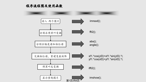
程序流程图及使用函数
读入两个图片
imread();
分别求傅里叶变换分别求幅度谱和相位谱
fft2();
感gle();
交换相位谱，重建复数矩阵傅里叶反变换
显示重构图片
第1页/共6页
xf1.*cos(yf2)+xf1.*sin(yf2).*i; yf1.*cos(xf2)+yf1.*sin(xf2).*i;
ifft2();
imshow();
二维FFT和交换图像相位谱
二维FFT：二维快速傅里叶变换是由一维FFT组合而成，其
第2页/共6页
程序运行结果
第3页/共6页
结论
交换相位谱，再反变换之后得到的图像内容与其相位谱对应的图像一致，我们可以得出相位谱决定图像结构的结论。明暗、灰度变化趋势等则在比较大的程度上取决于对应的幅度谱，幅度谱反映了图像整体上各个方向的频率分量的相对强度。
第4页/共6页
谢谢观看
第5页/共6页

1、下载文档前请自行甄别文档内容的完整性，平台不提供额外的编辑、内容补充、找答案等附加服务。
2、"仅部分预览"的文档,不可在线预览部分如存在完整性等问题,可反馈申请退款(可完整预览的文档不适用该条件!)。
3、如文档侵犯您的权益，请联系客服反馈,我们会尽快为您处理(人工客服工作时间：9:00-18:30)。

三．程序设计在matlab环境中，程序首先读取图像，然后调用直方图函数，设置相关参数，再输出处理后的图像。

书写程序时，首先读取图像，一般调用matlab自带的图像，如:cameraman图像；再调用相应的灰度均衡函数，设置参数；最后输出处理后的图像；3．浏览源程序并理解含义；4．运行，观察显示结果；5．结束运行，退出；五．实验结果观察matlab环境下图像灰度均衡结果及直方图分布。

(a)原始图像 (b)均衡化后图像(c)原始图像直方图 (d)均衡化后图像直方图六．实验报告要求1、给出实验原理过程及实现代码；2、输入一幅灰度图像，给出其灰度均衡结果，并进行灰度均衡化前后图像直方图分布对比分析。

实验二图像滤波实验2.1 3*3均值滤波一．实验目的1．熟悉matlab图像处理工具箱及均值滤波函数的使用；2．理解和掌握3*3均值滤波的方法和应用；二．实验设备1.PC机一台；2.软件matlab；三．程序设计在matlab环境中，程序首先读取图像，然后调用图像增强（均值滤波）函数，设置相关参数，再输出处理后的图像。

I = imread('cameraman.tif');figure,imshow(I);J=filter2(fspecial(‘average’,3),I)/255;figure,imshow(J);四．实验步骤1. 启动matlab双击桌面matlab图标启动matlab环境；2. 在matlab命令窗口中输入相应程序。

书写程序时，首先读取图像，一般调用matlab自带的图像，如:cameraman图像；再调用相应的图像增强（均值滤波）函数，设置参数；最后输出处理后的图像；3．浏览源程序并理解含义；4．运行，观察显示结果；5．结束运行，退出；五．实验结果观察matlab环境下原始图像经3*3均值滤波处理后的结果。

(a)原始图像 (b)3*3均值滤波处理后的图像图(3)六．实验报告要求输入一幅灰度图像，给出其图像经3*3均值滤波处理后的结果，然后对每一点的灰度值和它周围24个点，一共25个点的灰度值进行均值滤波，看看对25个点取均值与对9个点取中值进行均值滤波有什么区别？有没有其他的算法可以改进滤波效果。

实验2.2 3*3中值滤波一．实验目的1．熟悉matlab图像处理工具箱及中值滤波函数的使用；2．理解和掌握中值滤波的方法和应用；二．实验设备1.PC机一台；2.软件matlab；三．程序设计在matlab环境中，程序首先读取图像，然后调用图像增强（中值滤波）函数，设置相关参数，再输出处理后的图像。

I = imread('cameraman.tif');figure,imshow(I);J=medfilt2(I,[5,5]);figure,imshow(J);四．实验步骤1. 启动matlab双击桌面matlab图标启动matlab环境；2. 在matlab命令窗口中输入相应程序。

书写程序时，首先读取图像，一般调用matlab自带的图像，如:cameraman图像；再调用相应的图像增强（中值滤波）函数，设置参数；最后输出处理后的图像；3．浏览源程序并理解含义；4．运行，观察显示结果；5．结束运行，退出；五．实验结果观察matlab环境下原始图像经3*3中值滤波处理后的结果。

(a)原始图像 (b)3*3中值滤波处理后的图像图(4)六．实验报告要求输入一幅灰度图像，给出其图像经3*3中值滤波处理后的结果，然后对每一点的灰度值和它周围24个点，一共25个点的灰度值进行排序后取中值，然后该点的灰度值取中值。

看看对25个点取中值与对9个点取中值进行中值滤波有什么区别？实验三图像几何变换实验3.1 图像的缩放一．实验目的1．熟悉matlab图像处理工具箱及图像缩放函数的使用；2．掌握图像缩放的方法和应用；二．实验设备1.PC机一台；2.软件matlab；三．程序设计在matlab环境中，程序首先读取图像，然后调用图像缩放函数，设置相关参数，再输出处理后的图像。

I = imread('cameraman.tif');figure,imshow(I);scale = 0.5;J = imresize(I,scale);figure,imshow(J);四．实验步骤1. 启动matlab双击桌面matlab图标启动matlab环境；2. 在matlab命令窗口中输入相应程序。

书写程序时，首先读取图像，一般调用matlab自带的图像，如:cameraman图像；再调用相应的图像缩放函数，设置参数；最后输出处理后的图像；3．浏览源程序并理解含义；4．运行，观察显示结果；5．结束运行，退出；五．实验结果观察matlab环境下图像缩放后的结果。

(a)原始图像 (b)缩放后的图像图(5)六．实验报告要求输入一幅灰度图像，给出其图像缩放后的结果，然后改变缩放比率，观察图像缩放后结果柄进行分析。

实验3.2 图像旋转一．实验目的1．熟悉matlab图像处理工具箱及图像旋转函数的使用；2．理解和掌握图像旋转的方法和应用；二．实验设备1.PC机一台；2.软件matlab；三．程序设计在matlab环境中，程序首先读取图像，然后调用图像旋转函数，设置相关参数，再输出处理后的图像。

I = imread('cameraman.tif');figure,imshow(I);theta = 30;K = imrotate(I,theta); % Try varying the angle, theta.figure, imshow(K)四．实验步骤1. 启动matlab双击桌面matlab图标启动matlab环境；2. 在matlab命令窗口中输入相应程序。

书写程序时，首先读取图像，一般调用matlab自带的图像，如:cameraman图像；再调用相应的图像旋转函数，设置参数；最后输出处理后的图像；3．浏览源程序并理解含义；4．运行，观察显示结果；5．结束运行，退出；五．实验结果观察matlab环境下图像旋转后的结果。

(a)原始图像 (b)旋转后的图像图(7)六．实验报告要求输入一幅灰度图像，给出其图像旋转后的结果，然后改变旋转角度，观察图像旋转后结果柄进行分析。

实验四图像边缘检测实验4.1 边缘检测（Sobel、Prewitt、Log边缘算子）一．实验目的1．熟悉matlab图像处理工具箱及图像边缘检测函数的使用；2．理解和掌握图像边缘检测（Sobel、Prewitt、Log边缘算子）的方法和应用；二．实验设备1.PC机一台；2.软件matlab；三．程序设计在matlab环境中，程序首先读取图像，然后调用图像边缘检测（Sobel、Prewitt、Log边缘算子）函数，设置相关参数，再输出处理后的图像。

I = imread('cameraman.tif');J1=edge(I,'sobel');J2=edge(I,'prewitt');J3=edge(I,'log');subplot(1,4,1),imshow(I);subplot(1,4,2),imshow(J1);subplot(1,4,3),imshow(J2);subplot(1,4,4),imshow(J3);四．实验步骤1. 启动matlab双击桌面matlab图标启动matlab环境；2. 在matlab命令窗口中输入相应程序。

书写程序时，首先读取图像，一般调用matlab自带的图像，如:cameraman图像；再调用相应的边缘检测（Sobel边缘算子、Prewitt边缘算子、Log边缘算子）函数，设置参数；最后输出处理后的图像；3．浏览源程序并理解含义；4．运行，观察显示结果；5．结束运行，退出；五．实验结果观察经过图像边缘检测（Sobel、Prewitt、Log边缘算子）处理后的结果。

(a)原始图像 (b)Sobel边缘算子(c)Prewitt 边缘算子 (d)Log 边缘算子图(7)六．实验报告要求输入一幅灰度图像，给出其图像边缘检测（Sobel 、Prewitt 、Log 边缘算子）后的结果并进行分析对比。