[理学]中科大多核并行计算课件
中科大-并行计算讲义-并行计算机系统与结构模型

Intel Paragon系统框图
I/O部分
SCSI
计算
节点
节点
计算部分
计算 节点
……
服务部分 I/O部分
计算
服务
SCSI
节点
节点
节点
以太网
HIPPI 节点
计算 节点
计算 节点
……
计算 节点
服务 节点
SCSI 节点
FDDI
VME 节点
用户I/O
磁带
HIPPI 节点
计算 节点
计算 节点
……
计算 节点
CU
PE0
PE1
…
P E n-1
IN
M0
M1
…
M m-1
(b)共享存储阵列机
中科大-并行计算讲义-并行计算机系统与结构模 型
2021/1/21
6
阵列处理机的特点
• SIMD-单指令多数据流机
• 利用资源重复开拓计算空间的并行
• 同步计算--所有PE执行相同操作
• 适于特定问题(如有限差分、矩阵运算等) 求解
2021/1/21
10
Balance同构对称多处理机系统
80386CPU Weitek1167FPU
…
80386CPU Weitek1167FPU
存储器 8MB
…
存储器 8MB
64KB 高速缓存
…
64KB 高速缓存 系统总线
存储控制器
… 存储控制器
总线适配器 以太局域网
磁盘控制器
…
磁盘
磁盘
总线适配器 多总线
• 阵列处理机 分布存储 共享存储 流水线
• 向量处理机 并行向量机
并行计算PPT课件

C
Shell P
C
Shell P
互连网络
互连网络
(a)无共享
互连网络 共享磁盘
共享存储器 共享磁盘
(c)共享存储
(b)共享磁盘
2020/9/16
5
五种结构特性一览表
属性 结构类型 处理器类型 互连网络 通信机制 地址空间 系统存储器 访存模型 代表机器
2020/9/16
PVP MIMD 专用定制
SMP MIMD 商用
HP/Convex Exemplar)
分 布 存 储 器 NCC-NUMA (Cray T3E)
MIMD
DSM
NORMA
Cluster
(IBM SP2,DEC TruCluster Tandem Hymalaya,HP,
Microsoft Wolfpack,etc)
( 松散耦合)
(TreadMarks, Wind Tunnel, IVY,Shrimp,
etc.)
多计算机 (多 地 址 空 间 非 共 享 存 储 器 )
MPP (Intel TFLOPS)
( 紧耦合)
2020/9/16
7
SMP\MPP\机群比较
系统特征 节点数量(N) 节点复杂度 节点间通信
节点操作系统
支持单一系统映像 地址空间 作业调度 网络协议 可用性 性能/价格比 互连网络
S
MP
(Intel SHV,SunFire,DEC 8400, SGI PowerChallenge,IBMR60,etc.)
多处理机 ( 单地址空间
共享存储器 )
NUMA
COMA (KSR-1,DDM)
CC-NUMA
(Stanford Dash, SGI Origin 2000,Sequent NUMA-Q,
多核体系结构与并行编程模型计算机科学导论第八讲ppt课件

int retval; retval = curr; 1
– 原因: curr = curr+prev;1
对共享变
量的访问缺
乏约束
prev = retval; 1
curr = curr+prev;1 prev = retval; 1
28 t
共享变量并行编程模型
• 同步
– 同步是对线程执行的顺序进行强行限制的一种机 制,用来控制线程执行的相对顺序,可以有效解 决任何线程之间的冲突,而这些冲突有可能会导 致线程的执行出现异常行为
执行单元 缓存
单核结构
CPU状态 CPU状态 中断逻辑 中断逻辑
执行单元 缓存
超线程结构
多处理器结构
超线程技术充分利用执行
单元中的空闲资源,以便在 相同时间内完成更多工作
执行单元中的资源:内存
访问部件、算术运算部件和
浮点功能部件等
8
基本知识
• 单核结构与多核系统结构
CPU状态 中断逻辑
执行单元 缓存
P1: W(x)1
P2:
W(x)2
P3:
R(x)2 R(x)1
P4:
R(x)2 R(x)1
t 左图符合顺序
t 一致性:
t W(x)2先于W(x)1
发生
t
20
内存一致性模型
• 顺序一致性模型
– 比严格一致性弱的模型
– 在多处理器共享内存情况下,所有处理器的内存 访问操作都按照某个顺序逐个执行,并且每个处 理器执行的单个线程,严格按照程序规定的顺序 逐语句地进行内存访问操作
P1: W(x)1
t 左图不符合顺
P2:
W(x)2
t 序一致性:
中国科技大学GPU并行计算课件class7

GPU Architecture in detail and PerformanceOptimization (Part II)Bin ZHOU USTCAutumn, 20131 © 2012, NVIDIAAnnouncements •The Following Classes:–11/23 Review and Project Review–11/30 Final Exam + Project–12/07 12/14 Project–12/21 Project Defense–12/28 Or after that Course Close. •Project Source Code + Report + PPT •Important Time: Due to: 2013/12/18 24:00Contents•Last lecture Review + Continue•Optimization + Kepler New Things•Tools for Project3 © 2012, NVIDIAOptimizationMake the best or most effective use of asituation or resourceLast Lecture•General guideline•Occupancy Optimization•Warp branch divergence•Global memory access•Shared memory accessOutline•General guideline II•CPU-GPU Interaction Optimization•Kepler in detailTools•Winscp–Copy files from/to remote servers•Notepad++–Edit source files (with keyword highlighting)GENERAL GUIDELINE II8 © 2012, NVIDIAKernel Optimization WorkflowFind LimiterCompare topeak GB/s Memory optimization Compare topeak inst/sInstructionoptimizationConfigurationoptimizationMemory boundInstructionboundLatencybound Done!<< <<~ ~General Optimization Strategies: Measurement•Find out the limiting factor in kernel performance –Memory bandwidth bound (memory optimization)–Instruction throughput bound (instruction optimization) –Latency bound (configuration optimization)•Measure effective memory/instruction throughputMemory Optimization•If the code is memory-bound and effective memory throughput is much lower than the peak•Purpose: access only data that are absolutely necessary•Major techniques–Improve access pattern to reduce wasted transactions–Reduce redundant access: read-only cache, shared memoryInstruction Optimization•If you find out the code is instruction bound–Compute-intensive algorithm can easily become memory-bound if not careful enough–Typically, worry about instruction optimization after memory and execution configuration optimizations•Purpose: reduce instruction count–Use less instructions to get the same job done•Major techniques–Use high throughput instructions (ex. wider load)–Reduce wasted instructions: branch divergence, reduce replay (conflict), etc.Latency Optimization•When the code is latency bound–Both the memory and instruction throughputs are far from the peak•Latency hiding: switching threads–A thread blocks when one of the operands isn’t ready•Purpose: have enough warps to hide latency•Major techniques: increase active warps, increase ILPCPU-GPU INTERACTION14 © 2012, NVIDIAMinimize CPU-GPU data transferHost<->device data transfer has much lower bandwidth than global memory access.16 GB/s (PCIe x16 Gen3) vs 250 GB/s & 3.95 Tinst/s (GK110)Minimize transferIntermediate data can be allocated, operated, de-allocated directly on GPU Sometimes it’s even better to recompute on GPUMove CPU codes to GPU that do not have performance gains if it can reduce data transferGroup transferOne large transfer much better than many small onesOverlap memory transfer with computationPCI Bus 1.Copy input data from CPU memory to GPUmemoryPCI Bus 1.Copy input data from CPU memory to GPUmemory2.Load GPU code and execute itPCI Bus 1.Copy input data from CPU memory to GPUmemory2.Load GPU code and execute it3.Copy results from GPU memory to CPUmemory•T total=T HtoD+T Exec+T DtoH •More Overlap?HtoD Exec DtoH Stream 1HD1 HD2 E1 E2 DH1 DH2 Stream 2cudaStreamCreate(&stream1);cudaMemcpyAsync(dst1, src1, size, cudaMemcpyHostToDevice, stream1);kernel<<<grid, block, 0, stream1>>>(…);cudaMemcpyAsync(dst1, src1, size, stream1);cudaStreamSynchronize(stream1);cudaStreamCreate(&stream1);cudaStreamCreate(&stream2);cudaMemcpyAsync(dst1, src1, size, cudaMemcpyHostToDevice, stream1); cudaMemcpyAsync(dst2, src2, size, cudaMemcpyHostToDevice,stream2);kernel<<<grid, block, 0, stream1>>>(…);kernel<<<grid, block, 0, stream2>>>(…);cudaMemcpyAsync(dst1, src1, size, cudaMemcpyDeviceToHost, stream1); cudaMemcpyAsync(dst2, src2, size, cudaMemcpyDeviceToHost, stream2);cudaStreamSynchronize(stream1);cudaStreamSynchronize(stream2);KEPLER IN DETAIL23 © 2012, NVIDIAKepler•NVIDIA Kepler–1.31 tflops double precision–3.95 tflops single precision–250 gb/sec memorybandwidth–2,688 Functional Units(cores)•~= #1 on Top500 in 1997- KeplerKepler GK110 SMX vs Fermi SM3x perfPower goes down!New ISA Encoding: 255 Registers per Thread•Fermi limit: 63 registers per thread–A common Fermi performance limiter–Leads to excessive spilling•Kepler : Up to 255 registers per thread–Especially helpful for FP64 appsHyper-Q•Feature of Kepler K20 GPUs to increase application throughput by enabling work to be scheduled onto the GPU in parallel •Two ways to take advantage–CUDA Streams – now they really are concurrent –CUDA Proxy for MPI – concurrent CUDA MPIprocesses on one GPUBetter Concurrency SupportWork Distributor32 active gridsStream Queue Mgmt C B AR Q PZ Y XGrid Management UnitPending & Suspended Grids 1000s of pending gridsSMX SMX SMX SMXSM SM SM SM Work Distributor16 active gridsStream Queue MgmtC B AZ Y XR Q PCUDAGeneratedWorkFermiKepler GK110Fermi ConcurrencyFermi allows 16-way concurrency –Up to 16 grids can run at once–But CUDA streams multiplex into a single queue –Overlap only at stream edges P<<<>>> ;Q<<<>>> ;R<<<>>> A<<<>>> ; B<<<>>> ;C<<<>>> X<<<>>> ;Y<<<>>> ; Z<<<>>> Stream 1Stream 2Stream 3Hardware Work QueueA--B--C P--Q--R X--Y--ZKepler Improved ConcurrencyP<<<>>> ; Q<<<>>> ; R<<<>>>A <<<>>>;B <<<>>>;C<<<>>>X <<<>>>;Y <<<>>>; Z<<<>>>Stream 1Stream 2Stream 3Multiple Hardware Work QueuesA--B--CP--Q--R X--Y--ZKepler allows 32-way concurrencyOne work queue per stream Concurrency at full-stream level No inter-stream dependenciesCPU ProcessesShared GPUE FDCBACPU ProcessesShared GPUE FDCBACPU ProcessesShared GPUE FDCBACPU ProcessesShared GPUE FDCBACPU ProcessesShared GPUE FDCBACPU ProcessesShared GPUE FDCBACPU ProcessesShared GPUE FDCBAHyper-Q: Simultaneous MultiprocessE FDCBACPU ProcessesShared GPUCUDA ProxyClient – Server Software SystemWithout Hyper-QTime100500 G P U U t i l i z a t i o n % A B C D E FWith Hyper-Q Time 10050 0 G P U U t i l i z a t i o n % A A ABB BC CC D DDE E EF F FWhat is Dynamic Parallelism?The ability to launch new kernels from the GPU –Dynamically - based on run-time data–Simultaneously - from multiple threads at once–Independently - each thread can launch a different gridCPU GPU CPU GPU Fermi: Only CPU can generate GPU work Kepler: GPU can generate work for itselfCPU GPU CPU GPUWhat Does It Mean?Autonomous, Dynamic Parallelism GPU as Co-ProcessorNew Types of Algorithms•Recursive Parallel Algorithms like Quick sort •Adaptive Mesh Algorithms like Mandelbrot CUDA TodayCUDA on KeplerComputational Powerallocated to regions of interestGPU Familiar Programming Model__global__ void B(float *data) {do_stuff(data);X <<< ... >>> (data);Y <<< ... >>> (data);Z <<< ... >>> (data);cudaDeviceSynchronize();do_more_stuff(data);}ABCXYZ CPUint main() {float *data;setup(data);A <<< ... >>> (data);B <<< ... >>> (data);C <<< ... >>> (data);cudaDeviceSynchronize(); return 0;}__device__ float buf[1024]; __global__ void cnp(float *data){int tid = threadIdx.x;if(tid % 2)buf[tid/2] = data[tid]+data[tid+1];__syncthreads();if(tid == 0) {launch<<< 128, 256 >>>(buf); cudaDeviceSynchronize(); }__syncthreads();cudaMemcpyAsync(data, buf, 1024); cudaDeviceSynchronize();}Code Example Launch is per-threadand asynchronous__device__ float buf[1024]; __global__ void cnp(float *data) { int tid = threadIdx.x; if(tid % 2) buf[tid/2] = data[tid]+data[tid+1]; __syncthreads(); if(tid == 0) { launch<<< 128, 256 >>>(buf); cudaDeviceSynchronize();}__syncthreads();cudaMemcpyAsync(data, buf, 1024); cudaDeviceSynchronize();}Code Example Launch is per-threadand asynchronousCUDA primitives are per-blocklaunched kernels and CUDA objects like streams are visible to all threads in athread blockcannot be passed to child kernel__device__ float buf[1024]; __global__ void cnp(float *data) { int tid = threadIdx.x; if(tid % 2) buf[tid/2] = data[tid]+data[tid+1];__syncthreads();if(tid == 0) {launch<<< 128, 256 >>>(buf); cudaDeviceSynchronize();}__syncthreads();cudaMemcpyAsync(data, buf, 1024); cudaDeviceSynchronize();} Code Example Launch is per-threadand asynchronousCUDA primitives are per-blockSync includes all launches by any thread in the block__device__ float buf[1024]; __global__ void cnp(float *data) { int tid = threadIdx.x; if(tid % 2) buf[tid/2] = data[tid]+data[tid+1]; __syncthreads(); if(tid == 0) { launch<<< 128, 256 >>>(buf); cudaDeviceSynchronize(); } __syncthreads();cudaMemcpyAsync(data, buf, 1024); cudaDeviceSynchronize();}Code Example Launch is per-threadand asynchronousCUDA primitives are per-blockSync includes all launchesby any thread in the blockcudaDeviceSynchronize() does not imply syncthreads()__device__ float buf[1024]; __global__ void cnp(float *data){int tid = threadIdx.x;if(tid % 2)buf[tid/2] = data[tid]+data[tid+1];__syncthreads();if(tid == 0) {launch<<< 128, 256 >>>(buf); cudaDeviceSynchronize();}__syncthreads();cudaMemcpyAsync(data, buf, 1024); cudaDeviceSynchronize();}Code Example Launch implies membar(child sees parent state at time of launch)__device__ float buf[1024]; __global__ void cnp(float *data) { int tid = threadIdx.x; if(tid % 2)buf[tid/2] = data[tid]+data[tid+1];__syncthreads();if(tid == 0) {launch<<< 128, 256 >>>(buf); cudaDeviceSynchronize(); }__syncthreads();cudaMemcpyAsync(data, buf, 1024); cudaDeviceSynchronize(); } Code Example Launch implies membar(child sees parent state at time of launch) Sync implies invalidate(parent sees child writes after sync)。
中科大-并行计算讲义-并行计算机系统与结构模型PPT文档共37页

中科大-并行计算讲义-并行计算机系 统与结构模型
11、不为五斗米折腰。 12、芳菊开林耀,青松冠岩列。怀此 贞秀姿 ,卓为 霜下杰 。
13、归去来兮,田蜀将芜胡不归。 14、酒能祛百虑,菊为制颓龄。 15、春蚕收长丝,秋熟靡王税。
谢谢你的阅读
❖ 知识就是财富 ❖ 丰富你的人生
71、既然我已经踏上这条道路,那么,任何东西都不应妨碍我沿着这条路走下去。——康德 在旅行之际却是夜间的伴侣。——西塞罗 73、坚持意志伟大的事业需要始终不渝的精神。——伏尔泰 74、路漫漫其修道远,吾将上下而求索。——屈原 75、内外相应,言行相称。——韩非
中科大多核并行计算课件
• 划分重点在于:子问题易解,组合成原问题的解方便; • 有别于分治法
常见划分方法
• 均匀划分 • 方根划分
• 对数划分
• 功能划分(补)
2013-6-26
《并行与分布计算》 3 / Ch6
6.1.4 功能划分
方法: n个元素A[1..n]分成等长的p组,每组满足 某种特性。 示例: (m, n)选择问题(求出n个元素中前m个最小者)
2013-6-26
《并行与分布计算》 6 / Ch6
6.1.4 功能划分
2.2 奇偶归并示例:m=n=4 A=(2,4,6,8) B=(0,1,3,5)
(4, 4)2×(2, 2)4×(1, 1)
2 4 6
8 0 1 3
2 0 6
3 4 1 8
0 2 3
6 1 4 5
0 2 3
6 1 4 5
0 1 2 3 4 5 6 8 交叉比较
- 功能划分:要求每组元素个数必须大于m;
- 算法是基于Batcher排序网络,下面先介绍一些预备知识 :
1.Batcher比较器
2.奇偶归并及排序网络: 网络构造、奇偶归并网络、奇偶排序网络
3.双调归并及排序网络:
定义与定理、网络构造、双调归并网络、双调排序网络
《并行与分布计算》 4 / Ch6
1
3
Circuit for 4 inputs
1 2 3 4 15 21 28
《并行与分布计算》 24 / Ch6
6
10 10 5 + 11 10 10
Circuit for 4 inputs
+ 10 18 +
26
中科大-并行计算讲义第二讲-PC机群的搭建

重要特征
机群的各节点都是一个完整的系统,节点可以是工作站, 也可以是PC机或SMP机器; 互连网络通常使用商品化网络,如以太网、FDDI、光 通道等,部分商用机群也采用专用网络互连; 网络接口与节点的I/O总线松耦合相连; 各节点有一个本地磁盘; 各节点有自己的完整的操作系统。
这几行的意思是将服务器上的/home和/Cluster目录进行共享, 设置节点node1到node63可以访问,rw表示允许读和写(缺省为 只读)。这里要注意的一点是所有用到的主机名必须在文件 /etc/hosts中给出ip地址,例如: 192.168.0.11 node1
国家高性能计算中心(合肥) 2014-7-15 23
国家高性能计算中心(合肥)
2014-7-15
22
单一文件管理
(2) 设置共享目录:首先,在根目录下建立目录/home和/Cluster。
[node0]# mkdir home [node0]# mkdir Cluster
然后,在文件/etc/exports当中增加以下几行。
/home /Cluster …… /home /Cluster node1 (rw) node1 (rw) node63 (rw) node63 (rw)
国家高性能计算中心(合肥)
2014-7-15
5
分类
根据不同的标准,可有多种分类方式
针对机群系统的使用目的可将其分为三 类: 1. 高性能计算机群 2. 负载均衡机群 3. 高可用性机群
国家高性能计算中心(合肥)
2014-7-15
6
典型机群系统
Berkeley NOW Beowulf
理学中科大多核并行计算课件

使用HiPPI通道和开关构筑的 LAN主干网
超级计算机
帧缓冲器 RGB 显示器
300米 HiPPI 串行
Байду номын сангаас25米
存储器 服务器
25米 HiPPI HiPPI 交换开关
直至10千米
光纤扩展器
光纤扩展器
HiPPI 交换开关
25米
文件 服务器
串行
HiPPI
300米
300米 串行
大规模并行 处理系统
小型机
工作站 工作站
系统互连
▪ 不同带宽与间隔 的互连技术: 总线、SAN、LAN、MAN、WAN
100 Gb/s
MIN 或 交叉开关
10 Gb/s
局部总线 SCI
HiPPI
网络带宽
1 Gb/s
Myrinet 千兆位 以太网
100
I/O 总线
光纤 通道
FDDI
Mb/s
快速以太网
100 Base T
ATM
10 Mb/s
▪ 环网可完美嵌入到2-D环绕网中 ▪ 超立方网可完美嵌入到2-D环绕网中
嵌入〔2〕
1000
1001
1011
1010
1100
1101
1111
1110
0100
0101
0111
0110
0000
0001
0011
0010
0100
0110 0101
0111
0000
0010 0001
0011
1100
1110 1101
1111
1000
1010 1001
1011
静态互连网络特性比较
GPU计算 中国科技大学 并行算法 课件

据,访存速度很快 8192个32位字大小的寄存器文件供共享
To speed up access to the texture memory space
Device memory
Global, constant, texture memories
2.2 基本访存开销
存储器类型 寄存器 (Registers) 共享存储器 (Share Memory) 全局存储器 (Device Memory) 本地存储器 (Local Memory) 位置 芯片上 芯片上 设备上 设备上 是否被缓 存 不被缓存 不被缓存 不被缓存 不被缓存 被缓存 被缓存 访问速度 几乎没有额外延迟 同寄存器 400-600时钟周期 400-600时钟周期 被缓存时:同寄存器 未被缓存: 400-600时钟周期 被缓存时:同寄存器 未被缓存: 400-600时钟周期
PartⅠ Introduction to GPU
1. GPU的发展 2. CPU和GPU比较 3. GPU的应用和资源
2.1 单核时代的摩尔定律
CPU时钟频率每18个月翻一番 CPU制造工艺逐渐接近物理极限 功耗和发热成为巨大的障碍
2.2 GPU是多核技术的代表之一
在一块芯片上集成多个较低功耗的核心 单个核心频率基本不变(一般在1-3GHz) 设计重心转向到多核的集成技术
1.2 GPU的发展阶段
第一代GPU(1999年以前):部分功能从CPU分离,实现硬件 加速
《并行计算概述》PPT课件

Model
Project
Clip
Rasterize
2019/5/16
48
Processing One Data Set (Step 4)
Model
Project
Clip
Rasterize
The pipeline processes 1 data set in 4 steps
2019/5/16
49
Processing Two Data Sets (Step 1)
2019/5/16
23
并行化方法
域分解(Domain decomposition) 任务分解(Task decomposition) 流水线(Pipelining)
2019/5/16
24
域分解
First, decide how data elements should be divided among processors
2019/5/16
并行计算
3
并行的层次
程序级并行
粗
子程序级并行
并 行
语句级并行
粒 度
操作级并行
微操作级并行
细
2019/5/16
4
FLOPS
Floating point number Operations Per Second --每个时钟周期执行浮点运算的次数
理论峰值=CPU主频*每时钟周期执行浮点运 算数*CPU数目
并行计算 Parallel Computing
基本概念
如何满足不断增长的计算力需求?
用速度更快的硬件,也就是减少每一条指令所 需时间
优化算法(或者优化编译) 用多个处理机(器)同时解决一个问题
中国科技大学GPU并行计算课件class8
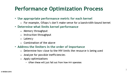
Performance Optimization Process•Use appropriate performance metric for each kernel –For example, Gflops/s don’t make sense for a bandwidth-bound kernel •Determine what limits kernel performance–Memory throughput–Instruction throughput–Latency–Combination of the above•Address the limiters in the order of importance–Determine how close to the HW limits the resource is being used–Analyze for possible inefficiencies–Apply optimizations•Often these will just fall out from how HW operatesPresentation Outline•Identifying performance limiters•Analyzing and optimizing :–Memory-bound kernels–Instruction (math) bound kernels–Kernels with poor latency hiding–Register spilling•For each:–Brief background–How to analyze–How to judge whether particular issue is problematic–How to optimize–Some cases studies based on “real-life” application kernels •Most information is for Fermi GPUsNotes on profiler•Most counters are reported per Streaming Multiprocessor (SM)–Not entire GPU–Exceptions: L2 and DRAM counters• A single run can collect a few counters–Multiple runs are needed when profiling more counters•Done automatically by the Visual Profiler•Have to be done manually using command-line profiler•Counter values may not be exactly the same for repeated runs –Threadblocks and warps are scheduled at run-time–So, “two counters being equal” usually means “two counters within a small delta”•See the profiler documentation for more informationIdentifying Performance LimitersLimited by Bandwidth or Arithmetic?•Perfect instructions:bytes ratio for Fermi C2050:–~4.5 : 1 with ECC on–~3.6 : 1 with ECC off–These assume fp32 instructions, throughput for other instructions varies •Algorithmic analysis:–Rough estimate of arithmetic to bytes ratio•Code likely uses more instructions and bytes than algorithm analysis suggests:–Instructions for loop control, pointer math, etc.–Address pattern may result in more memory fetches–T wo ways to investigate:•Use the profiler (quick, but approximate)•Use source code modification (more accurate, more work intensive)Analysis with Profiler•Profiler counters:–instructions_issued, instructions_executed•Both incremented by 1per warp•“issued” includes replays, “executed” does not–gld_request, gst_request•Incremented by1 per warp for each load/store instruction•Instruction may be counted if it is “predicated out”–l1_global_load_miss, l1_global_load_hit, global_store_transaction•Incremented by 1per L1 line(line is 128B)–uncached_global_load_transaction•Incremented by1 per group of 1, 2, 3, or 4 transactions•Better to look at L2_read_request counter (incremented by 1 per 32 bytes, per GPU)•Compare:–32 * instructions_issued/* 32 = warp size */–128B * (global_store_transaction+ l1_global_load_miss)A Note on Counting Global Memory Accesses•Load/store instruction count can be lower than the number of actual memory transactions–Address pattern, different word sizes•Counting requests from L1 to the rest of the memory system makes the most sense–Caching-loads: count L1 misses–Non-caching loads and stores: count L2 read requests•Note that L2 counters are for the entire chip, L1 counters are per SM•Some shortcuts, assuming “coalesced” address patterns:–One 32-bit access instruction-> one 128-byte transaction per warp–One 64-bit access instruction-> two 128-byte transactions per warp–One 128-bit access instruction-> four 128-byte transactions per warpAnalysis with Modified Source Code•Time memory-only and math-only versions of the kernel –Easier for codes that don’t have data-dependent control-flow oraddressing–Gives you good estimates for:•Time spent accessing memory•Time spent in executing instructions•Comparing the times for modified kernels–Helps decide whether the kernel is mem or math bound–Shows how well memory operations are overlapped with arithmetic •Compare the sum of mem-only and math-only times to full-kernel timetimeMemory-boundGood mem-mathoverlap: latency not aproblem(assuming memorythroughput is not lowcompared to HW theory)mem mathfull mem math fullMath-boundGood mem-mathoverlap: latency not aproblem(assuming instructionthroughput is not lowcompared to HW theory)Memory-boundGood mem-mathoverlap: latency not aproblem(assuming memorythroughput is not lowcompared to HW theory) timemem mathfull mem mathfull mem math full Math-boundGood mem-mathoverlap: latency not aproblem(assuming instructionthroughput is not lowMemory-boundGood mem-math overlap: latency not a problem(assuming memory throughput is not low compared to HW theory)BalancedGood mem-math overlap: latency not a problem(assuming memory/instr throughput is not low compared to HW theory)timemem mathfull mem mathfull mem mathfull mem math fullMemory and latency boundPoor mem-math overlap:latency is a problem Math-boundGood mem-mathoverlap: latency not aproblem(assuming instructionthroughput is not lowMemory-boundGood mem-math overlap: latency not a problem(assuming memory throughput is not low compared to HW theory)BalancedGood mem-math overlap: latency not a problem(assuming memory/instr throughput is not low compared to HW theory)timeSource Modification•Memory-only:–Remove as much arithmetic as possible•Without changing access pattern•Use the profiler to verify that load/store instruction count is the same •Store-only:–Also remove the loads•Math-only:–Remove global memory accesses–Need to trick the compiler:•Compiler throws away all code that it detects as not contributing to stores•Put stores inside conditionals that always evaluate to false–Condition should depend on the value about to be stored (prevents other optimizations)–Condition outcome should not be known to the compilerSource Modification for Math-only __global__ void fwd_3D( ..., int flag){...value = temp + coeff* vsq; if( 1 == value * flag )g_output[out_idx] = value; }If you compare only the flag, the compiler may move the computation into the conditional as wellSource Modification and Occupancy •Removing pieces of code is likely to affect register count–This could increase occupancy, skewing the results–See slide 23 to see how that could affect throughput •Make sure to keep the same occupancy–Check the occupancy with profiler before modifications –After modifications, if necessary add shared memory to match the unmodified kernel’s occupancykernel<<< grid, block, smem,...>>>(...)•Analysis:–Instr:byte ratio = ~2.66•32*18,194,139 / 128*1,708,032–Good overlap between math and mem:•2.12 ms of math-only time (13%) are not overlapped with mem–App memory throughput: 62 GB/s•HW theory is 114 GB/s , so we’re off•Conclusion:–Code is memory-bound –Latency could be an issue too–Optimizations should focus on memorythroughput first•math contributes very little to total time (2.12 out of 35.39ms)•3DFD of the wave equation, fp32•Time (ms):–Full-kernel:35.39–Mem-only:33.27–Math-only:16.25•Instructions issued:–Full-kernel:18,194,139–Mem-only:7,497,296–Math-only:16,839,792•Memory access transactions:–Full-kernel:1,708,032–Mem-only:1,708,032–Math-only:•Analysis:–Instr:byte ratio = ~2.66•32*18,194,139 / 128*1,708,032–Good overlap between math and mem:•2.12 ms of math-only time (13%) are not overlapped with mem–App memory throughput: 62 GB/s•HW theory is 114 GB/s , so we’re off•Conclusion:–Code is memory-bound –Latency could be an issue too–Optimizations should focus on memorythroughput first•math contributes very little to total time (2.12out of 35.39ms )•3DFD of the wave equation, fp32•Time (ms):–Full-kernel:35.39–Mem-only:33.27–Math-only:16.25•Instructions issued:–Full-kernel:18,194,139–Mem-only:7,497,296–Math-only:16,839,792•Memory access transactions:–Full-kernel:1,708,032–Mem-only:1,708,032–Math-only:Summary: Limiter Analysis•Rough algorithmic analysis:–How many bytes needed, how many instructions •Profiler analysis:–Instruction count, memory request/transaction count •Analysis with source modification:–Memory-only version of the kernel–Math-only version of the kernel–Examine how these times relate and overlapOptimizations for Global MemoryMemory Throughput Analysis•Throughput: from application point of view–From app point of view:count bytes requested by the application –From HW point of view:count bytes moved by the hardware–The two can be different•Scattered/misaligned pattern: not all transaction bytes are utilized•Broadcast: the same small transaction serves many requests•Two aspects to analyze for performance impact:–Addressing pattern–Number of concurrent accesses in flightMemory Throughput Analysis•Determining that access pattern is problematic:–Profiler counters: access instruction count is significantly smaller thantransaction count•gld_request< ( l1_global_load_miss+ l1_global_load_hit) * ( word_size/ 4B )•gst_request< 4 * l2_write_requests* ( word_size/ 4B )•Make sure to adjust the transaction counters for word size (see slide 8)–App throughput is much smaller than HW throughput•Use profiler to get HW throughput•Determining that the number of concurrent accesses is insufficient:–Throughput from HW point of view is much lower than theoreticalConcurrent Accesses and Performance•Increment a 64M element array–T wo accesses per thread (load then store, but they are dependent)•Thus, each warp (32 threads) has one outstanding transaction at a time•Tesla C2050, ECC on, theoretical bandwidth: ~120 GB/sSeveral independent smalleraccesses have the same effectas one larger one.For example:Four 32-bit ~= one 128-bitOptimization: Address Pattern•Coalesce the address pattern–128-byte lines for caching loads–32-byte segments for non-caching loads, stores– A warp’s address pattern is converted to transactions•Coalesce to maximize utilization of bus transactions•Refer to CUDA Programming Guide / Best Practices Guide / Fundamental Opt. talk •Try using non-caching loads–Smaller transactions (32B instead of 128B)•more efficient for scattered or partially-filled patterns•Try fetching data from texture–Smaller transactions and different caching–Cache not polluted by other gmem loadsOptimizing Access Concurrency•Have enough concurrent accesses to saturate the bus –Need (mem_latency)x(bandwidth) bytes in flight (Little’s law)–Fermi C2050 global memory:•400-800cycle latency, 1.15 GHz clock, 144 GB/s bandwidth, 14 SMs•Need 30-50128-byte transactions in flight per SM•Ways to increase concurrent accesses:–Increase occupancy•Adjust threadblock dimensions–T o maximize occupancy at given register and smem requirements•Reduce register count (-maxrregcount option, or __launch_bounds__)–Modify code to process several elements per threadCase Study: Access Pattern 1•Same 3DFD code as in the previous study•Using caching loads (compiler default):–Memory throughput: 62 /74 GB/s for app / hw–Different enough to be interesting•Loads are coalesced:–gld_request== ( l1_global_load_miss + l1_global_load_hit )•There are halo loads that use only 4threads out of 32–For these transactions only 16bytes out of 128are useful•Solution: try non-caching loads ( -Xptxas–dlcm=cg compiler option)–Performance increase of 7%•Not bad for just trying a compiler flag, no code change–Memory throughput: 66 /67 GB/s for app / hwCase Study: Accesses in Flight•Continuing with the FD code–Throughput from both app and hw point of view is 66-67 GB/s–Now 30.84out of 33.71 ms are due to mem–1024concurrent threads per SM•Due to register count (24 per thread)•Simple copy kernel reaches ~80% of achievable mem throughput at this thread count •Solution: increase accesses per thread–Modified code so that each thread is responsible for 2output points •Doubles the load and store count per thread, saves some indexing math•Doubles the tile size -> reduces bandwidth spent on halos–Further 25% increase in performance•App and HW throughputs are now 82and 84 GB/s, respectively•Kernel from climate simulation code–Mostly fp64 (so, at least 2transactions per mem access)•Profiler results:–gld_request:72,704–l1_global_load_hit:439,072–l1_global_load_miss:724,192•Analysis:–L1 hit rate: 37.7%–16 transactions per load instruction•Indicates bad access pattern(2are expected due to 64-bit words)•Of the 16, 10 miss in L1 and contribute to mem bus traffic•So, we fetch 5x more bytes than needed by the app•Looking closer at the access pattern:–Each thread linearly traverses a contiguous memory region–Expecting CPU-like L1 caching•Remember what I said about coding for L1 and L2•(Fundamental Optimizations, slide 11)–One of the worst access patterns for GPUs•Solution:–Transposed the code so that each warp accesses a contiguous memory region–2.17transactions per load instruction–This and some other changes improved performance by 3xSummary: Memory Analysis and Optimization•Analyze:–Access pattern:•Compare counts of access instructions and transactions•Compare throughput from app and hw point of view–Number of accesses in flight•Look at occupancy and independent accesses per thread•Compare achieved throughput to theoretical throughput–Also to simple memcpy throughput at the same occupancy•Optimizations:–Coalesce address patterns per warp (nothing new here), consider texture–Process more words per thread (if insufficient accesses in flight to saturate bus)–Try the 4 combinations of L1 size and load type (caching and non-caching)–Consider compressionOptimizations for Instruction ThroughputPossible Limiting Factors•Raw instruction throughput–Know the kernel instruction mix–fp32, fp64, int, mem, transcendentals, etc. have different throughputs •Refer to the CUDA Programming Guide / Best Practices Guide–Can examine assembly, if needed:•Can look at PTX (virtual assembly), though it’s not the final optimized code•Can look at post-optimization machine assembly for GT200 (Fermi version coming later)•Instruction serialization–Occurs when threads in a warp issue the same instruction in sequence •As opposed to the entire warp issuing the instruction at once•Think of it as “replaying” the same instruction for different threads in a warp –Some causes:•Shared memory bank conflicts•Constant memory bank conflictsInstruction Throughput: Analysis•Profiler counters (both incremented by 1 per warp):–instructions executed:counts instructions encoutered during execution –instructions issued:also includes additional issues due to serialization –Difference between the two: issues that happened due to serialization,instr cache misses, etc.•Will rarely be 0, cause for concern only if it’s a significant percentage ofinstructions issued•Compare achieved throughput to HW capabilities–Peak instruction throughput is documented in the Programming Guide –Profiler also reports throughput:•GT200: as a fraction of theoretical peak for fp32 instructions•Fermi: as IPC (instructions per clock)Instruction Throughput: Optimization•Use intrinsics where possible ( __sin(), __sincos(),__exp(), etc.)–Available for a number of math.h functions–2-3 bits lower precision, much higher throughput•Refer to the CUDA Programming Guide for details–Often a single instruction, whereas a non-intrinsic is a SW sequence •Additional compiler flags that also help (select GT200-level precision):–-ftz=true: flush denormals to 0–-prec-div=false: faster fp division instruction sequence (some precision loss) –-prec-sqrt=false: faster fp sqrt instruction sequence (some precision loss)•Make sure you do fp64 arithmetic only where you mean it:–fp64 throughput is lower than fp32–fp literals without an “f” suffix ( 34.7 ) are interpreted as fp64 per C standardSerialization: Profiler Analysis•Serialization is significant if–instructions_issued is significantly higher than instructions_executed •Warp divergence–Profiler counters: divergent_branch, branch–Compare the two to see what percentage diverges•However, this only counts the branches, not the rest of serialized instructions •SMEM bank conflicts–Profiler counters:•l1_shared_bank_conflict: incremented by 1per warp for each replay–double counts for 64-bit accesses•shared_load, shared_store: incremented by 1per warp per instruction –Bank conflicts are significant if both are true:•instruction throughput affects performance•l1_shared_bank_conflict is significant compared to instructions_issuedSerialization: Analysis with Modified Code •Modify kernel code to assess performance improvement if serialization were removed–Helps decide whether optimizations are worth pursuing •Shared memory bank conflicts:–Change indexing to be either broadcasts or just threadIdx.x–Should also declare smem variables as volatile•Prevents compiler from “caching” values in registers•Warp divergence:–change the condition to always take the same path–Time both paths to see what each costsSerialization: Optimization•Shared memory bank conflicts:–Pad SMEM arrays•For example, when a warp accesses a 2D array’s column•See CUDA Best Practices Guide, Transpose SDK whitepaper –Rearrange data in SMEM•Warp serialization:–Try grouping threads that take the same path•Rearrange the data, pre-process the data•Rearrange how threads index data (may affect memory perf)Case Study: SMEM Bank Conflicts• A different climate simulation code kernel, fp64•Profiler values:–Instructions:•Executed / issued:2,406,426/ 2,756,140•Difference:349,714(12.7% of instructions issued were “replays”)–GMEM:•Total load and store transactions:170,263•Instr:byte ratio: 4–suggests that instructions are a significant limiter (especially since there is a lot of fp64 math)–SMEM:•Load / store:421,785/ 95,172•Bank conflict:674,856(really 337,428because of double-counting for fp64)–This means a total of 854,385SMEM access instructions, (421,785+95,172+337,428), 39% replays •Solution:–Pad shared memory array: performance increased by 15%•replayed instructions reduced down to 1%Instruction Throughput: Summary•Analyze:–Check achieved instruction throughput–Compare to HW peak (but must take instruction mix intoconsideration)–Check percentage of instructions due to serialization •Optimizations:–Intrinsics, compiler options for expensive operations–Group threads that are likely to follow same execution path –Avoid SMEM bank conflicts (pad, rearrange data)Optimizations for LatencyLatency: Analysis•Suspect if:–Neither memory nor instruction throughput rates are close to HW theoretical rates–Poor overlap between mem and math•Full-kernel time is significantly larger than max{mem-only, math-only}•Two possible causes:–Insufficient concurrent threads per multiprocessor to hide latency•Occupancy too low•T oo few threads in kernel launch to load the GPU–elapsed time doesn’t change if problem size is increased (and with it the number of blocks/threads)–T oo few concurrent threadblocks per SM when using __syncthreads()•__syncthreads() can prevent overlap between math and mem within the same threadblockMath-only time Memory-only time Full-kernel time, one large threadblock per SM Kernel where most math cannot be executed until all data is loaded by the threadblockMath-only time Memory-only time Full-kernel time, two threadblocks per SM (each half the size of one large one)Full-kernel time, one large threadblock per SM Kernel where most math cannot be executed until all data is loaded by the threadblockLatency: Optimization•Insufficient threads or workload:–Increase the level of parallelism (more threads)–If occupancy is already high but latency is not being hidden:•Process several output elements per thread –gives more independent memory and arithmetic instructions (which get pipelined)•Barriers:–Can assess impact on perf by commenting out __syncthreads()•Incorrect result, but gives upper bound on improvement–Try running several smaller threadblocks•Think of it as “pipelining” blocks•In some cases that costs extra bandwidth due to halos•Check out Vasily Volkov’s talk 2238 at GTC 2010 for a detailed treatment:–“Better Performance at Lower Latency”Register SpillingRegister Spilling•Compiler “spills” registers to local memory when register limit is exceeded –Fermi HW limit is 63 registers per thread–Spills also possible when register limit is programmer-specified•Common when trying to achieve certain occupancy with -maxrregcount compiler flag or __launch_bounds__ in source–lmem is like gmem, except that writes are cached in L1•lmem load hit in L1-> no bus traffic•lmem load miss in L1-> bus traffic (128 bytes per miss)–Compiler flag –Xptxas–v gives the register and lmem usage per thread •Potential impact on performance–Additional bandwidth pressure if evicted from L1–Additional instructions–Not always a problem, easy to investigate with quick profiler analysisRegister Spilling: Analysis•Profiler counters:l1_local_load_hit, l1_local_load_miss •Impact on instruction count:–Compare to total instructions issued•Impact on memory throughput:–Misses add 128 bytes per warp–Compare 2*l1_local_load_miss count to gmem access count(stores + loads)•Multiply lmem load misses by 2: missed line must have been evicted ->store across bus•Comparing with caching loads: count only gmem misses in L1•Comparing with non-caching loads: count all loadsOptimization for Register Spilling•Try increasing the limit of registers per thread–Use a higher limit in –maxrregcount, or lower thread count for __launch_bounds__–Will likely decrease occupancy, potentially making gmem accesses lessefficient–However, may still be an overall win –fewer total bytes being accessed in gmem•Non-caching loads for gmem–potentially fewer contentions with spilled registers in L1•Increase L1 size to 48KB–default is 16KB L1 / 48KB smemRegister Spilling: Case Study•FD kernel, (3D-cross stencil)–fp32, so all gmem accesses are 4-byte words •Need higher occupancy to saturate memory bandwidth –Coalesced, non-caching loads•one gmem request = 128 bytes•all gmem loads result in bus traffic–Larger threadblocks mean lower gmem pressure •Halos (ghost cells) are smaller as a percentage•Aiming to have 1024concurrent threads per SM –Means no more than 32 registers per thread–Compiled with –maxrregcount=32•10th order in space kernel (31-point stencil)–32 registers per thread : 68 bytes of lmem per thread : upto1024 threads per SM•Profiled counters:–l1_local_load_miss= 36inst_issued= 8,308,582–l1_local_load_hit= 70,956gld_request= 595,200–local_store= 64,800gst_request= 128,000•Conclusion: spilling is not a problem in this case–The ratio of gmem to lmem bus traffic is approx 8,444 : 1 (hardly any bus traffic is due to spills)•L1 contains most of the spills (99.9% hit rate for lmem loads)–Only 1.6% of all instructions are due to spills•Comparison:–42 registers per thread : no spilling : upto768 threads per SM•Single 512-thread block per SM : 24% perf decrease•Three 256-thread blocks per SM : 7% perf decrease•12th order in space kernel (37-point stencil)–32 registers per thread : 80 bytes of lmem per thread : upto1024 threads per SM •Profiled counters:–l1_local_load_miss= 376,889inst_issued= 10,154,216–l1_local_load_hit= 36,931gld_request= 550,656–local_store= 71,176gst_request= 115,200•Conclusion: spilling is a problem in this case–The ratio of gmem to lmem bus traffic is approx 7 : 6 (53% of bus traffic is due to spilling)•L1 does not contain the spills (8.9% hit rate for lmem loads)–Only 4.1% of all instructions are due to spills•Solution: increase register limit per thread–42 registers per thread : no spilling : upto768 threads per SM–Single 512-thread block per SM : 13%perf increase–Three 256-thread blocks per SM : 37%perf increase。
中科大多核并行计算课件

1 消息传递库(Message-Passing Libraries)
PVM和MPI间的主要差别: (1)PVM是一个自包含的系统, 而MPI不是. MPI依赖于支持 它的平台提供对进程的管理和I/O功能. 而PVM本身就包含 这些功能. (2) MPI对消息传递提供了更强大的支持. (3) PVM不是一个标准, 这就意味着PVM可以更方便、更频 繁地进行版本更新. MPI和PVM在功能上现在正趋于相互包含. 例如, MPI-2增 加了进程管理功能, 而现在的PVM也提供了更多的群集通 信函数.
国家高性能计算中心(合肥)
2 消息传递方式
关于通信模式, 用户需要理解的有三个方面:
共有多少个进程?
进程间如何同步? 如何管理通信缓冲区? 现在的消息传递系统多使用如下三种通信方式: 同步的消息传递 (Synchronous Message Passing)
阻塞的消息传递 (Blocking Message Passing)
非阻塞的消息传递 (Nonblocking Message Passing)
国家高性能计算中心(合肥)
三种通信模式的比较
2 消息传递方式
通信事件 发送开始的条件 发送返回意味着 接收开始的条件 接收返回意味着 语义 同步通信 双方都到达了发送和接收点 消息已被收到 双方都到达了发送和接收点 消息已被收到 明确 阻塞的通信 发送方到达发送点 消息已被发送完 接收方到达发送点 消息已被收到 二者之间 需要 非阻塞的通信 发送方到达发送点 通知完系统某个消息要被发送 接收方到达接收点 通知完系统某个消息要被接收 需做错误探测 需要
国家高性能计算中心(合肥)
1 消息传递库(Message-Passing Libraries)
- 1、下载文档前请自行甄别文档内容的完整性,平台不提供额外的编辑、内容补充、找答案等附加服务。
- 2、"仅部分预览"的文档,不可在线预览部分如存在完整性等问题,可反馈申请退款(可完整预览的文档不适用该条件!)。
- 3、如文档侵犯您的权益,请联系客服反馈,我们会尽快为您处理(人工客服工作时间:9:00-18:30)。
如果将3-立方的每个顶点代之以一个环就构成了如图(d)所示 的3-立方环,此时每个顶点的度为3,而不像超立方那样节点 度为n。
节点 N
SAN(e.g.Myrinet)
I/O总线,系统总线
接口
LAN(e.g.以太网,FDDI)
系统 II
国家高性能计算中心(合肥)
2019/5/13
7
网络性能指标
节点度(Node Degree):射入或射出一个节点的边 数。在单向网络中,入射和出射边之和称为节点度。
网络直径(Network Diameter): 网络中任何两个 节点之间的最长距离,即最大路径数。
核武器数值模拟、航天器设计、基因测序等。 需求类型:计算密集、数据密集、网络密集。 美国HPCC计划(1993):重大挑战性课题,3T
性能 美国Petaflops研究项目:Pflop/s。 美国ASCI计划(1996):核武器数值模拟。
国家高性能计算中心(合肥)
2019/5/13
Hale Waihona Puke 4第一章并行计算机系统及结构模型
对剖宽度(Bisection Width) :对分网络各半所必须 移去的最少边数
对剖带宽( Bisection Bandwidth):每秒钟内,在最小 的对剖平面上通过所有连线的最大信息位(或字节)数
如果从任一节点观看网络都一样,则称网络为对称的 (Symmetry)
国家高性能计算中心(合肥)
多核并行计算
Multicore Parallel Computing
主讲人 徐 云
并行计算——结构•算法•编程
第一篇 并行计算的基础
第一章 并行计算机系统及其结构模型 第二章 当代并行机系统:SMP、MPP和Cluster 第三章 并行计算性能评测
国家高性能计算中心(合肥)
2019/5/13
(b)Illiac网孔 2019/5/13
(c)2-D环绕 11
静态互连网络(3)
二叉树:
除了根、叶节点,每个内节点只与其父节点和两个子节点相连。
节点度为3,对剖宽度为1,而树的直径为2log N 1 如果尽量增大节点度数,则直径缩小为2,此时就变成了星形
网络,其对剖宽度为 N / 2
国家高性能计算中心(合肥)
2019/5/13
9
静态互连网络(1)
一维线性阵列(1-D Linear Array):
并行机中最简单、最基本的互连方式, 每个节点只与其左、右近邻相连,也叫二近邻连接, N个节点用N-1条边串接之,内节点度为2,直径为
N-1,对剖宽度为1 当首、尾节点相连时可构成循环移位器,在拓扑结
1.1 并行计算
1.1.1 并行计算与计算科学 1.1.2 当代科学与工程问题的计算需求
1.2 并行计算机系统互连
1.2.1 系统互连 1.2.2 静态互联网络 1.2.3 动态互连网络 1.2.4 标准互联网络
1.3 并行计算机系统结构
1.3.1 并行计算机结构模型 1.3.2 并行计算机访存模型
FDDI
Mb/s
快速以太网
100 Base T
ATM
10 Mb/s
IsoEnet 以太网 10 Base T
总线或开关
SAN
LAN
MAN
WAN
国家高性能计算中心(合肥)
2019/5/13
6
局部总线、I/O总线、SAN和LAN
节点 1
P
M
处理器总线
局部总线,存储器总线
I/O
SCSI 磁盘
桥
系统 I
节点 2
1.3.1 并行计算机结构模型 1.3.2 并行计算机访存模型
1.4 多核处理器架构
国家高性能计算中心(合肥)
2019/5/13
3
并行计算、计算科学、计算需求
并行计算:并行机上所作的计算,又称高性能 计算或超级计算。
计算科学:计算物理、计算化学、计算生物等 科学与工程问题的需求:气象预报、油藏模拟、
节点度为4,网络直径为
2,( N对剖1) 宽度为
N
在垂直方向上带环绕,水平方向呈蛇状,就变成Illiac网孔了,
节点度恒为4,网络直径为
,N 而1 对剖宽度为
2N
垂直和水平方向均带环绕,则变成了2-D环绕(2-D Torus),
节点度恒为4,网络直径为
,对2剖 N宽/ 2度 为
2N
(a)2-D网孔 国家高性能计算中心(合肥)
构上等同于环,环可以是单向的或双向的,其节点 度恒为2,直径或为 (双向环)或为N-1(单向 环),对剖宽度为2 N / 2
国家高性能计算中心(合肥)
2019/5/13
10
静态互连网络(2)
N N 二维网孔(2-D Mesh):
每个节点只与其上、下、左、右的近邻相连(边界节点除外),
2019/5/13
8
静态互连网络 与动态互连网络
静态互连网络:处理单元间有着固定连接的一类网络, 在程序执行期间,这种点到点的链接保持不变;典型的 静态网络有一维线性阵列、二维网孔、树连接、超立方 网络、立方环、洗牌交换网、蝶形网络等
动态网络:用交换开关构成的,可按应用程序的要求动 态地改变连接组态;典型的动态网络包括总线、交叉开 关和多级互连网络等。
1.4 多核处理器架构
国家高性能计算中心(合肥)
2019/5/13
5
系统互连
不同带宽与距离的互连技术: 总线、SAN、LAN、MAN、WAN
100 Gb/s
MIN 或 交叉开关
10 Gb/s
局部总线 SCI
HiPPI
网络带宽
1 Gb/s
Myrinet 千兆位 以太网
100
I/O 总线
光纤 通道
2
第一章并行计算机系统及结构模型
1.1 并行计算
1.1.1 并行计算与计算科学 1.1.2 当代科学与工程问题的计算需求
1.2 并行计算机系统互连
1.2.1 系统互连 1.2.2 静态互联网络 1.2.3 动态互连网络 1.2.4 标准互联网络
1.3 并行计算机系统结构
传统二叉树的主要问题是根易成为通信瓶颈。胖树节点间的通 路自叶向根逐渐变宽。
(a)二叉树
(b)星形连接
(c)二叉胖树
国家高性能计算中心(合肥)
2019/5/13
12
静态互连网络(4)
超立方 :
一个n-立方由 N 2n 个顶点组成,3-立方如图(a)所示;4-立 方如图(b)所示,由两个3-立方的对应顶点连接而成。