ANSYS CFD管道流体分析算例Fluid11

合集下载

ansys fluent中文版流体计算工程案例详解

ansys fluent中文版流体计算工程案例详解ANSYS Fluent是一种流体计算动力学软件，可用于解决各种流体力学问题。

本文将详细介绍ANSYS Fluent中文版的流体计算工程案例，包括案例的基本背景、模拟过程和结果分析。

这些案例旨在帮助用户深入了解ANSYS Fluent的使用方法和流体计算工程实践。

一个典型的案例是流体在管道中的流动。

该案例背景是，一根长直管道内有水流动，管道的直径为0.1米，长度为10米。

水的初始速度为1 m/s，管道的壁面是光滑的，管道两端的压差为100Pa。

现在需要使用ANSYS Fluent模拟该流体流动过程，并进一步分析不同参数对流动的影响。

首先，在ANSYS Fluent中创建一个新的仿真项目，并选择“仿真”模块。

在界面上点击“新建”按钮，在弹出的对话框中填写相应的参数，例如案例名称、计算器类型和尺寸单位。

点击“确定”后，进入模拟设置页面。

首先，需要定义获得流动场稳定解所需的物理模型和求解方法。

在“物理模型”选项卡中，选择“连续相”和“非恒定模型”。

在“湍流模型”中选择某种适合的模型，例如k-ε模型。

在“重力”选项卡中，定义流体的密度和重力加速度。

接下来，在“模型”选项卡中，定义管道的几何和边界条件。

选择“管道”作为流体领域的几何模型，并定义长度、直径和内壁面的润滑系数。

在“边界”选项卡中，定义管道两端的入口和出口条件，例如速度和压力。

将管道两端的压力差设置为100Pa，在入口处设置水的初始速度为1 m/s。

在出口处选择“出流”边界条件。

完成几何和边界条件的定义后，点击“模拟”选项卡进入模拟设置界面。

在“求解控制”中，设置计算时间步长和迭代次数。

选择合适的网格划分方法，并进行网格划分。

点击“网格”选项卡，选择合适的网格类型，并进行网格划分。

在划分网格后，可以使用“导入”按钮导入网格文件，并进行网格优化。

完成设置后，点击“计算”按钮开始进行模拟计算。

在计算过程中，可以实时观察流体场的变化情况，并通过Fluent Post-processing工具进行结果分析。

ANSYS流体第4章flotran流体分析典型工程实例

第4 章FLOTRAN流体分析典型工程实例ANSYS程序中的FLOTRAN CFD流体分析是一个用于分析二维及三维流体流动场的先进工具。

本章重点通过实例讲解介绍FLOTRAN CFD流体分析在工程上的一些典型应用。

本章要点如何解决流体力学问题FLOTRAN流体分析典型工程实例本章案例三维U型管道速度场的数值模拟实际生活中射流现象的数值模拟4.1 如何解决流体力学问题在流体力学的研究中，常用的方法有理论研究方法、数值计算方法和实验研究方法。

理论研究方法的特点是：能够清晰、普遍地揭示出流动的内在规律，但该方法目前只局限于少数比较简单的理论模型。

研究更复杂更符合实际的流动一般采用数值计算方法，它的特点就是能够解决理论研究方法无法解决的复杂流动问题，如常见的航空工程、气象预报、水利工程、环境污染预报、星云演化过程等。

实验研究方法的特点就是结果可靠，但其局限性在于相似准侧不能全部满足、尺寸限制、边界影响等。

数值计算方法和实验研究方法相比，它所需的费用和时间都比较少，并且有较高的精度，但它要求对问题的物理特性有足够的了解（通过实验方法了解），并能建立较精确的描述方程组（通过理论分析）。

对于流体力学的数值模拟常采用的步骤如下。

（1）建立力学模型通过流动分析，采用合理的假设与简化，建立力学模型。

假设与简化：连续介质与不连续介质；理想流体与粘性流体；不可压缩流体与可压缩流体；定常流动与非定常流动。

（2）建立数学模型根据力学模型，建立描述力学模型的数学方程组，并利用无量钢化、量纲分析、引进新的物理参数、经验或半经验公式等方法对基本方程组进行简化，得到相应流动的求解方程组，再根据具体的流动条件确定流动的初始条件和边界条件。

描写流体运动的两种方法：拉格朗日方法和欧拉方法。

（3）求解方法●准确解法：解析解●近似解法：近似解、数值解●实验解法：相似解（4）求解结果速度分布、压力分布、合力、阻力、能量耗散等物理量的求解结果。

ANSYS教学算例集FL_工艺注射混合管流场分析

物理模型设置
• 表达式求值 Ø 点击选择【Evaluate】标签 Ø 在T后输入栏中填入300[K] Ø 点击【Evaluate Expression】
物理模型设置
• 调整材料属性 Ø 选择Outline标签，展开Materials，双击下面Water属性，进入到设置 Ø 切换至【Material Properties】标签 Ø 展开【Transport Properties】 Ø 选择【Dynamic Viscosity】 Ø 在【Dynamic Viscosity】下选择【Dynamic Viscosity】栏 Ø 点击右边Expression按钮，转换至表达式输入模式 Ø 将VisT填入表达式栏中 Ø 点击【OK】
• 保存case文件 Ø 选择【File】>【Save Case As】，在【File name】中写入InjectMixer，单击【Save料属性 Ø 在主菜单下选择【Insert】>【Expressions，Functions and Variables】>
写出CFX-Solver求解输入文件（.def）
• 菜单栏中单击Define Run 。 • 保存名称为InjectMixer.def的文件。 • 点击Save保存。 • 选择【File】>【Close】退出CFX-Pre。 • 选择弹出对话框中的【Save&Close】。
CFX-Solver求解设置
Energy】。 Ø 点击【OK】 • 创建流场进口边界 Ø 在Outline下的InjectMxier行单击右键，选择【Insert】>【Boundary】选项，在Name栏后填入“side inlet”，点击【OK】。 Ø 进入到Basic Settings设置栏中，保持【Boundary Type】>【Inlet】。选择【Location】>【side inlet】。 Ø 其余具体设置参数

ANSYS／FLOTRAN流体动力学(CFD)分析

Intro-9
目标
Module Objective
在完成本章学习后，在完成本章学习后，我们应该对流体动力学分析的基本概念有所了解，并知道它的基本分类。有所了解，并知道它的基本分类。
第一讲、第一讲、FLOTRAN CFD 分析的概念第二讲、第二讲、 FLOTRAN 分析的种类第三讲、层流分析第四讲、第四讲、紊流分析第五讲、第五讲、热分析第六讲、第六讲、可压缩流分析第七讲、第七讲、非牛顿流分析第八讲、多组份传输分析第八讲、
ANSYS培训教程 – 版本 5.5 – XJTU MSSV By: Haich Gao (011001) Intro-4
2001年10月1日
目录
设置命令（第三章 FLOTRAN设置命令（续）设置命令
Guidelines
十三、设定FLOTRAN自由度松弛系数设定自由度松弛系数十四、设定FLOTRAN流体性质松弛因子十四、设定流体性质松弛因子十五、设置FLOTRAN分析的自由度限值十五、设置分析的自由度限值十六、选择FLOTRAN各自由度相应的求解器十六、选择各自由度相应的求解器十七、十七、对FLOTRAN各求解器的控制各求解器的控制十八、设置FLOTRAN湍流模型的一些常数十八、设置湍流模型的一些常数十九、重新设定FLOTRAN各分析参数的值十九、重新设定各分析参数的值二十、控制FLOTRAN面积积分的阶次二十、控制面积积分的阶次二十一、二十一、FLOTRAN多组份疏运分析的设置及控制多组份疏运分析的设置及控制二十二、定义FLOTRAN的重启动（续算）控制的重启动（二十二、定义的重启动续算）二十三、设置并执行一个零迭代FLOTRAN分析二十三、设置并执行一个零迭代分析

ANSYS／FLOTRAN流体动力学CFD分析

2001年10月1日
ANSYS培训教程 – 版本 5.5 – XJTU MSSV By: Haich Gao (011001)
Intro-15
非牛顿流分析
Objective
T-2. FLOTRAN 分析的种类
应力与应变率之间成线性关系的这种理论并不能足以解释很多流体的流动，对于这种非牛顿流体，ANSYS程序提供了三中粘性模式和一个用户自定义子程序。
2001年10月1日
ANSYS培训教程 – 版本 5.5 – XJTU MSSV By: Haich Gao (011001)
Intro-20
FLUID141单元
Objective
T2-1. FLOTRAN单元的特点
FLUID141单元具有下列特征：维数：二维形状：四节点四边形或三节点三角形自由度：速度、压力、温度、紊流动能、紊流能量耗散、多达六种流体的各自质量所占的份额
ANSYS培训教程 – 版本 5.5 – XJTU MSSV By: Haich Gao (011001) Intro-3
2001年10月1日
目录
第三章
Guidelines
FLOTRAN设置命令（续）
十三、设定FLOTRAN自由度松弛系数十四、设定FLOTRAN流体性质松弛因子十五、设置FLOTRAN分析的自由度限值十六、选择FLOTRAN各自由度相应的求解器十七、对FLOTRAN各求解器的控制十八、设置FLOTRAN湍流模型的一些常数十九、重新设定FLOTRAN各分析参数的值二十、控制FLOTRAN面积积分的阶次二十一、FLOTRAN多组份疏运分析的设置及控制二十二、定义FLOTRAN的重启动（续算）控制二十三、设置并执行一个零迭代FLOTRAN分析

ANSYS流体分析

第一章 FLOTRAN 计算流体动力学(CFD)分析概述FLOTRAN CFD 分析的概念ANSYS程序中的FLOTRAN CFD分析功能是一个用于分析二维及三维流体流动场的先进的工具，使用ANSYS中用于FLOTRAN CFD分析的FLUID 141和FLUID 142 单元，可解决如下问题：作用于气动翼(叶)型上的升力和阻力超音速喷管中的流场弯管中流体的复杂的三维流动同时，FLOTRAN还具有如下功能：计算发动机排气系统中气体的压力及温度分布研究管路系统中热的层化及分离使用混合流研究来估计热冲击的可能性用自然对流分析来估计电子封装芯片的热性能对含有多种流体的(由固体隔开)热交换器进行研究FLOTRAN 分析的种类FLOTRAN可执行如下分析：层流或紊流传热或绝热可压缩或不可压缩牛顿流或非牛顿流多组份传输这些分析类型并不相互排斥，例如，一个层流分析可以是传热的或者是绝热的，一个紊流分析可以是可压缩的或者是不可压缩的。

层流分析层流中的速度场都是平滑而有序的，高粘性流体（如石油等）的低速流动就通常是层流。

紊流分析紊流分析用于处理那些由于流速足够高和粘性足够低从而引起紊流波动的流体流动情况，ANSYS中的二方程紊流模型可计及在平均流动下的紊流速度波动的影响。

如果流体的密度在流动过程中保持不变或者当流体压缩时只消耗很少的能量，该流体就可认为是不可压缩的，不可压缩流的温度方程将忽略流体动能的变化和粘性耗散。

热分析流体分析中通常还会求解流场中的温度分布情况。

如果流体性质不随温度而变，就可不解温度方程。

在共轭传热问题中，要在同时包含流体区域和非流体区域（即固体区域）的整个区域上求解温度方程。

在自然对流传热问题中，流体由于温度分布的不均匀性而导致流体密度分布的不均匀性，从而引起流体的流动，与强迫对流问题不同的是，自然对流通常都没有外部的流动源。

可压缩流分析对于高速气流，由很强的压力梯度引起的流体密度的变化将显著地影响流场的性质，ANSYS对于这种流动情况会使用不同的解算方法。

ANSYS CFD管道流体分析算例Fluid11

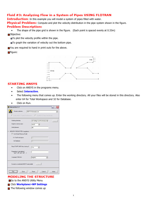
Fluid #3: Analyzing Flow in a System of Pipes USING FLOTRANIntroduction: In this example you will model a system of pipes filled with water.Physical Problem: Compute and plot the velocity distribution in the pipe system shown in the figure. Problem Description:∙The shape of the pipe grid is shown in the figure. (Each point is spaced evenly at 0.33m)O bjective:T o plot the velocity profile within the pipe.T o graph the variation of velocity out the bottom pipe.Y ou are required to hand in print outs for the above.F igure:STARTING ANSYS∙Click on ANSYS in the programs menu.∙Select Interactive.∙The following menu that comes up. Enter the working directory. All your files will be stored in this directory. Also enter 64 for Total Workspace and 32 for Database.∙Click on Run.MODELING THE STRUCTUREG o to the ANSYS Utility MenuClick Workplane>WP SettingsThe following window comes up∙Check the Cartesian and Grid Only buttons∙Enter the values shown in the figure above.∙Go to the ANSYS Main Menu∙In this problem we will model the pipe grid and then apply fluid flow to it.∙Click Preprocessor>-Modeling-> and create the pipe grid as shown below.∙Hint: You can use key points and then create the areaThe modeling of the problem is done.ELEMENT PROPERTIESSELECTING ELEMENT TYPE:∙Click Preprocessor>Element Type>Add/Edit/Delete... In the 'Element Types' window that opens click on Add...The following window opens:∙Type 1 in the Element type reference number.∙Click on Flotran CFD and select 2D Flotran 141. Click OK. Close the 'Element types' window.∙So now we have selected Element type 1 to be a Flotran element. The component will now be modeled using the principles of fluid dynamics. This finishes the selection of element type.DEFINE THE FLUID PROPERTIES:∙Go to Preprocessor>Flotran Set Up>Fluid Properties.∙On the box, shown below, make sure the first two input fields read Constant, and then click on OK. Another box will appear. Fill in the values as shown below, then click OK.∙Now we’re ready to de fine the Material PropertiesMATERIAL PROPERTIES∙Go to the ANSYS Main Menu∙Click Preprocessor>Material Props>Material Models. The following window will appear∙As displayed, choose CFD>Density. The following window appears.∙Fill in 1000 to set the density of Water. Click OK.∙Now choose CFD>Viscosity. The following window appears:∙Fill in 1 to set the viscosity of Water. Click OK∙Now the Material 1 has the properties defined in the above table so the Material Models window may be closed. MESHING:DIVIDING THE CHANNEL INTO ELEMENTS:∙Go to Preprocessor>Meshing>Size Cntrls>ManualSize>Global>Size. In the window that comes up type0.025 in the field for 'Element edge length'.∙Click on OK. Now when you mesh the figure ANSYS will automatically create a mesh, whose elements have a edge length of 0.025 m.∙Now go to Preprocessor>Meshing>Mesh>Areas>Free. Click Pick All. The mesh will look like the following.BOUNDARY CONDITIONS AND CONSTRAINTS∙Go to Preprocessor>Loads>Define Loads>Apply>Fluid CFD>Velocity>On lines. Pick the left edge of the block and Click OK. The following window comes up.∙Enter 0.5 in the VX value field and click OK. The 0.5 corresponds to the velocity of 0.5 meters per second of air flowing into the pipe grid.∙Repeat the above and set the velocity into the upper pipe as -1 meter/second. This is because theflow is traveling to the left, or the negative direction.∙Then, set the Velocity to ZERO along all of the edges of the pipes. This is because of the “No Slip Condition”(VX=VY=0 for all sides)∙Go to Main Menu>Preprocessor>Loads>Define Loads>Apply>Fluid CFD>Pressure DOF>On Lines. Pick the bottom pipe outlet and click OK.∙Once all the Boundary Conditions have been applied, the pipe grid will look like this:∙Now the Modeling of the problem is done.SOLUTION∙Go to ANSYS Main Menu>Solution>Flotran Set Up>Execution Ctrl.∙The following window appears. Change the first input field value to 50, as shown. No other changes are needed. Click OK.∙Go to Solution>Run FLOTRAN.∙Wait for ANSYS to solve the problem.∙Click on OK and close the 'Information' window.POST-PROCESSING∙Plotting the velocity distribution…∙Go to General Postproc>Read Results>Last Set.∙Then go to General Postproc>Plot Results>Contour Plot>Nodal Solution. The following window appears:∙Select DOF Solution and Velocity VSUM and Click OK.∙This is what the solution should look like:∙Next, go to Main Menu>General Postproc>Plot Results>Vector Plot>Predefined.The following window will appear:Select OK to accept the defaults. This will display the vector plot of the velocity gradient.。

ANSYS流体第4节flotran流体分析典型工程实例

第4 章FLOTRAN流体分析典型工程实例ANSYS程序中的FLOTRAN CFD流体分析是一个用于分析二维及三维流体流动场的先进工具。

本章重点通过实例讲解介绍FLOTRAN CFD流体分析在工程上的一些典型应用。

理论研究方法的特点是：能够清晰、普遍地揭示出流动的内在规律，但该方法目前只局限于少数比较简单的理论模型。

实验研究方法的特点就是结果可靠，但其局限性在于相似准侧不能全部满足、尺寸限制、边界影响等。

对于流体力学的数值模拟常采用的步骤如下。

（1）建立力学模型通过流动分析，采用合理的假设与简化，建立力学模型。

假设与简化：连续介质与不连续介质；理想流体与粘性流体；不可压缩流体与可压缩流体；定常流动与非定常流动。

描写流体运动的两种方法：拉格朗日方法和欧拉方法。

ansys cfd入门指南计算流体力学基础与应用

ansys cfd入门指南计算流体力学基础与应用1. 引言计算流体力学（Computational Fluid Dynamics，简称CFD）是一种利用数值方法解决流动问题的工程学科。

它通过数值模拟和计算来研究流体在各种条件下的运动和相互作用。

而ANSYS CFD则是CFD领域中一种常用的软件工具，它提供了广泛的功能和强大的计算能力，使工程师能够更好地理解和优化流体问题。

2. 概述ANSYS CFDANSYS CFD是由ANSYS公司开发的一套用于CFD分析的软件。

它采用了计算网格和数值方法，通过将流体领域离散为有限数量的小块，利用数值求解方法来模拟流体的运动。

ANSYS CFD具有较高的准确性和可靠性，可以用于解决各种复杂的流体力学问题。

3. CFD基础知识为了更好地理解ANSYS CFD的工作原理，我们需要了解一些CFD的基础知识。

我们需要了解流体力学的基本方程：质量守恒方程、动量守恒方程和能量守恒方程。

这些方程描述了流体在不同条件下的运动和相互作用。

4. ANSYS CFD的功能ANSYS CFD提供了丰富的功能，可以满足不同应用场景的需求。

它支持不同类型的流体，包括压缩性流体和非压缩性流体。

它支持不同的边界条件和初始条件，以模拟各种实际情况。

ANSYS CFD还提供了不同的数值方法和求解器，以提高计算效率和准确性。

5. ANSYS CFD的应用领域ANSYS CFD可以应用于各种领域的流体问题研究和优化。

它可以用于飞行器的气动设计和优化，以提高飞行性能和燃油效率。

它也可以用于汽车工程中的空气动力学分析，以改善汽车的操控性和燃油经济性。

ANSYS CFD还可以应用于能源领域的风力发电和涡轮机械的设计与分析。

6. ANSYS CFD的优势和局限性虽然ANSYS CFD具有强大的功能和广泛的应用领域，但它也存在一些局限性。

ANSYS CFD需要较高的计算资源和时间，对计算机的性能要求较高。

ANSYS CFD在某些复杂流动问题中可能存在数值稳定性和收敛性的挑战。

ANSYS模拟风荷载流体力学计算

关于计算流体力学主要有以下几个主要问题大家比较关心一、关于瞬态计算的问题：计算瞬态设置参数与稳态不同，主要设置的参数为：1．FLDATA1,SOLU,TRAN,1 设置为瞬态模式2．FLDATA4,TIME,STEP,0.02, 自定义时间步时间间隔0.02秒3．FLDATA4,TIME,TEND,0.1, 设置结束时间0。

1秒4．FLDATA4,TIME,GLOB,10, 设置每个时间步多少次运算5．fldata4a,time,appe,0.02 设置记录时间间隔6．SET,LIST,2 查看结果7．SET,LAST 设为最后一步8．ANDATA,0.5, ,2,1,6,1,0,1 动态显示结果以上为瞬态和稳态不同部分的设置和操作，特别是第五步。

为了动态显示开始到结束时间内气流组织的情况，还是花了我们很多时间来找到这条命令。

如果你是做房间空调送风计算的，这项对你来说非常好，可以观察到从开空调机到稳定状态的过程。

二．关于建模的问题大家主要关心的建模问题是模型的导入和导出，及存在的一些问题。

这些问题主要体现在：1．AUTOCAD建模导出后的格式与ANSYS兼容的只有SAT格式。

PROE可以是IGES格式或SAT格式。

当然还有其它格式，本人使用的限于正版软件，只有上述两种格式。

SAT格式可由PROE中导出为IGES格式。

ANSYS默认的导入模型为IGES格式的图形模型。

2．使用AUTOCAD一般绘制界面比较复杂的拉伸体非常方便。

如果是不规则体，用PROE 和ANSYS都比较方便，当然本人推荐用ANSYS本身的建模功能。

对于PROE，因为它的功能强大，本人推荐建立很复杂的模型如变截面不规则曲线弯管（如血管）。

3．导入过程中会出现默认选项和自定义选项，一般本人推荐使用自定义选项，以避免一些操作带来的问题。

有时出现显示只有线而没有面颜色的问题，可以用命令：/FACET,NORML 来解决这个问题。

三．关于网格化的问题。

ansys流体分析FLOTRAN

一、FLOTRAN CFD 分析的概念二、 FLOTRAN 分析的种类
1、层流分析 2、紊流分析 3、热分析 4、可压缩流分析 5、非牛顿流分析 6、多组份传输分析
2001年10月1日 2019/2/24
*ANSYS培训教程 – 版本 5.5 – XJTU MSSV By: Haich Gao (011001)
2001年本 5.5 – XJTU MSSV By: Haich Gao (011001)
Intro-16
非牛顿流分析
Objective
T-2. FLOTRAN 分析的种类
应力与应变率之间成线性关系的这种理论并不能足以解释很多流体的流动，对于这种非牛顿流体，ANSYS程序提供了三中粘性模式和一个用户自定义子程序。
2001年10月1日 2019/2/24
*ANSYS培训教程 – 版本 5.5 – XJTU MSSV By: Haich Gao (011001)
Intro-6
目录
第五章
Guidelines
FLOTRAN层流和湍流分析算例
一、问题描述二、分析方法及假定三、几何尺寸及流体性质四、分析过程
第1步：进入ANSYS 第2步：设置分析选择第3步：定义单元类型第4步：生成分析区域的几何面第5步：定义单元形状第6步：划分有限元网格第7步：生成并应用新的工具栏按钮第8步：施加边界条件第9步：求解层流
ANSYS程序中的FLOTRAN CFD分析功能是一个用于分析二维及三维流体流动场的先进的工具，使用 ANSYS 中用于 FLOTRAN CFD分析的FLUID 141和FLUID 142 单元，可解决如下问题：作用于气动翼(叶)型上的升力和阻力超音速喷管中的流场弯管中流体的复杂的三维流动同时，FLOTRAN还具有如下功能：计算发动机排气系统中气体的压力及温度分布研究管路系统中热的层化及分离使用混合流研究来估计热冲击的可能性用自然对流分析来估计电子封装芯片的热性能对含有多种流体的(由固体隔开)热交换器进行研究

ansys-fluids流体计算的例子

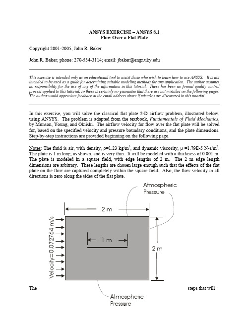
ANSYS EXERCISE – ANSYS 8.1Flow Over a Flat PlateCopyright 2001-2005, John R. BakerJohn R. Baker; phone: 270-534-3114; email: jbaker@This exercise is intended only as an educational tool to assist those who wish to learn how to use ANSYS. It is not intended to be used as a guide for determining suitable modeling methods for any application. The author assumes no responsibility for the use of any of the information in this tutorial. There has been no formal quality control process applied to this tutorial, so there is certainly no guarantee that there are not mistakes on the following pages. The author would appreciate feedback at the email address above if mistakes are discovered in this tutorial.In this exercise, you will solve the classical flat plate 2-D airflow problem, illustrated below, using ANSYS. The problem is adapted from the textbook, Fundamentals of Fluid Mechanics, by Munson, Young, and Okiishi. The airflow velocity for flow over the flat plate will be solved for, based on the specified velocity and pressure boundary conditions, and the plate dimensions. Step-by-step instructions are provided beginning on the following page.Notes: The fluid is air, with density, ρ=1.23 kg/m3, and dynamic viscosity, μ =1.79E-5 N-s/m2. The plate is 1 m long, as shown, and is very thin. It will be modeled with a thickness of 0.001 m. The plate is modeled in a square field, with edge lengths of 2 m. The 2 m edge length dimensions are arbitrary. These lengths are chosen large enough such that the effects of the flat plate on the flow are captured completely within the square field. Also, the flow velocity in all directions is zero along the sides of the flat plate.The steps that willbe followed, after launching ANSYS, are:Preprocessing:1. Change Preferences2. Change Jobname.3. Define element type. (Fluid141 element, which is a 2-D element for fluid analysis.)4. Define the fluid. (Air – SI Units.)5. Create keypoints.6. Create areas.7. Specify meshing controls / Mesh the areas to create nodes and elements.8. Zoom in to see flat plate region (optional).Solution:9. Specify boundary conditions.10. Specify number of solution iterations.11. Solve.Postprocessing:11. Plot the x-direction velocity (VX) distribution.12. List VX at Nodes.Exit13. Exit the ANSYS program, saving all data._____________________________________________________________________________ Notes:•It is assumed in this tutorial that the user has already launched ANSYS and is working in the Graphical User Interface (GUI).•The menu picks needed to perform all required tasks are specified in italics in the step-by-step instructions below. It is sometimes more convenient to enter certain commands directly at the command line. The method of direct command line entry, however, is not emphasized in this exercise. Primarily, in this exercise, the analysis will be performed using menu picks from the ANSYS Graphical User Interface.SUGGESTION: As you work through this exercise, on the ANSYS Toolbar click on “SAVE_DB” often!At any point, if you want to resume from the previous time the model was saved, simply click on “RESUM_DB” on this same Toolbar. Any information entered since the last save will be lost, but this is a nice feature in the event that you make an input mistake, and are unsure of how to correct it.Note: Most of the required tasks are performed using menu picks from the ANSYS GUI, as specified in italics in the step-by-step instructions below. It is sometimes more convenient, however, to enter certain commands directly at the command line. The command line is seen on the screen.The Main Menu is on the left side of the screen.The method of direct command line entry is used in some cases in this exercise, whenever this method seems more convenient than using menu picks.Often, as an alternative, an input file, known as a “batch file”, is created, which is simply an ASCII text file containing a string of ANSYS commands in the appropriate order. ANSYS can read in this file as if it were a program, and perform the analysis in “batch mode”, without ever opening up the Graphical User Interface. The batch file option is not covered in this exercise.There are a number of ways to model a system and perform an analysis in ANSYS. The steps below present only one method.Preprocessing:1. Change Preferences. Main Menu -> Preferences -> FLOTRAN CFD -> OK2. Change jobname. At the upper left-hand corner of the screen:File -> Change JobnameEnter “flatplate”, and click on “OK”.3. Define element type:Preprocessor -> Element Type -> Add/Edit/DeleteClick on “Add”. The “Library of Element Types” box appears, as shown. Highlight “FLOTRAN CFD”, and “2D FLOTRAN 141”. Click on “OK”, then “Close”.4. Define fluid properties: Preprocessor -> FLOTRAN Set Up ->Fluid PropertiesOn the box, shown below, change the first two input fields to “AIR-SI”, and then click on “OK”. Another box will appear. Accept all defaults on that box by clicking on “OK”.5. Create keypoints:There are several options available for creating the basic geometry. The method that will be employed involves creating “keypoints”, then generating two separate areas, with corners defined by the keypoints.Preprocessor -> -Modeling- Create -> Keypoints -> In Active CS…Fill in the fields as shown below, then click “APPLY”. When you click on “Apply”, the command is issued to create keypoint number 1 at (x,y,z)=(-1,1,0). Note that when the Z field is left blank, in this case, the blank space defaults to zero, which is desired. Since you clicked on “Apply”, instead of “OK”, then the keypoint creation box remains open.Create keypoint number 2 at (x,y,z)=(0,1,0), using the input shown below. After entering the input, again, click on “APPLY”:Create 12 total keypoints in the same manner. The locations for all 12 are shown in the following table. When the final keypoint is created, click on “OK” instead of “APPLY”.“OK” issues the command and also closes the keypoint creation box.Keypoint Number X-Location Y-Location1 -1 12 0 13 1 14 -0.5 05 0 06 0.5 0-0.0017 -0.5-0.0018 0-0.0019 0.510 -1 -111 0 -112 1 -1Before moving on, it is probably a good idea to check the keypoint locations. Along thetop toolbar choose:List -> Keypoint -> Coordinates Only.A box should open up with the keypoint location information. If any keypoint is not inthe correct location, at this point, you can just re-issue the keypoint creation command for that particular keypoint. To do this, choose:Preprocessor -> -Modeling- Create -> Keypoints -> In Active CS…Fill in the correct information for that particular keypoint in the box, and click “OK”. The keypoint will be moved to the correct location. If you have some keypoint incorrectly numbered above number 12, this will not cause a problem. Just be sure you have keypoint numbers 1 thru 12 located correctly.You can close the box listing the keypoint locations, by clicking, in that listing box, on “File-> Close”.6. Create areas:It may be a good idea to save your model at this point, by clicking “SAVE_DB”on the ANSYS Toolbar. Now, if you make a mistake from which you do not know howto recover, just click on “RESUM_DB”, and the model will resume from the point of the last save.We will create two separate areas. One is the left half of the flow field, and the other is the right half. We will do this by defining areas, as outlined below, using the defined keypoints as corners of the areas. The figure below shows the end result, exceptthe figure shows an extremely exaggerated thickness of the flat plate. This is done forclarity. The black dots denote keypoints, and the circled numbers denote the keypoint numbers.In creating the areas, it is probably easiest to use the direct command line entry approach. At the command line, type in, as shown below: a,1,2,5,4,7,8,11,10Hit “Enter”, and the left half of the flow field is generated as an area, defined by the keypoints entered with the “a” command. Now, create the right half, by typing, at the command line: a,2,3,12,11,8,9,6,5After hitting “Enter”, the right side is generated. Note that, although we have created the flow field in two halves, the entire 2 m x 2 m field could have been produced as a single square. Then, the flat plate could have been cut out of that square. However, the method being employed will produce a line of “nodes” protruding vertically from the center of the flat plate, and this will be desirable when the fluid velocity results are compared to the analytical solution. At this time, the horizontal flat plate appears in the graphics window as a single line, because it is so thin. The plot in the graphics window should appear as:7. Specify Mesh Size Controls / Mesh the Model.There are a number of ways to perform this step, but for this exercise, the procedure has been automated, and will involve typing only a single word, below. The actual method employed would involve entering 24 commands at the command line. Because of the possibility of typographical errors, however, for this exercise, this step has been automated, using the “macro” option within ANSYS. A macro has been created. It is a text file named mshfield.mac. It is available for download on the website from which this tutorial was downloaded. The file, mshfield.mac, should be copied to your ANSYS working directory. The commands in the macro are discussed in the Appendix, at the end of these instructions. However, to execute all of the required commands (assuming you have the file “mshfield.mac” stored in your current ANSYS working directory), all that is needed is to type, at the command line:mshfieldThen, hit “Enter”. All of the necessary commands should be executed, and the mesh should appear, as shown in the following figure on the next page. The requiredcommands are listed in the appendix.GUI with Finite Element Mesh in Graphics Window8. Zoom in to see the flat plate (optional)This step is not necessary, but it may be helpful to you to see the flat plate geometry, and the fine mesh near the plate. If you wish to zoom in, first, it may be best to turn off the X-Y-Z Axis “Triad” display, as it is really just in the way. We know that we defined our model so that +x is to the right on the screen, and +y is upward. To turn off the X-Y-Z Axis “Triad” display, on the menu across the very top of the GUI choose:PltCtrls -> Window Controls -> Window OptionsA box appears. Change the [/TRIAD] option to “Not Shown”, and then click “OK”.Then, back to the menu across the very top of the GUI, select:PltCtrls -> Pan, Zoom, Rotate…The “Pan-Zoom-Rotate” box below appears. On that box, select “Box Zoom”Then, in the graphics window, press the left mouse button, and drag to producea box near the center of the flow area. Then, click once with the left mousebutton, and you will see a zoomed view of the region around the plate, withthe fine mesh. At any time, to return to the full model view, on the “Pan-Zoom-Rotate” box, click on “Fit” (near the bottom of the box).Solution:9. Specify boundary conditions.In Step 6, there is a sketch of the geometry, with an exaggerated thickness for the flat plate. You may want to refer to this figure and the figure on page 1, during the boundary condition specification. The boundary condition specification steps are outlined below, in steps 9a thru 9e, where VX denotes X-direction flow velocity, and VY denotes Y-direction flow velocity. Before beginning the specifications, it is probably best to plot the lines, without showing the areas, for better clarity. On the menu along the very top of the GUI, select:Plot -> LinesYou should then see colored lines, which are the boundaries of the areas. Unless you are zoomed in, the flat plate will probably appear as a single horizontal line. Although not necessary, you may also want to turn on “Keypoint Numbering”. To do this, again on the very top menu, choose: PltCtrls -> NumberingZoomed View of PlateThe box below opens. Click on the box to the right of “Keypoint numbers” to toggle from “Off” to “On”. Then, click on “OK”. If you have the lines plotted, then the keypoint numbers should also show.9a) Specification of VX Value and VY=0 on the line connecting keypoints 1 and 10.One way to do this is to choose, and the ANSYS Main Menu:Solution -> Define Loads-> Apply->Fluid/CFD-> Velocity -> On LinesA picking menu appears, as shown (below, left). Click on the far left vertical line (theline which connects keypoints 1 and 10), and it should highlight. In the picking menu, choose “OK”. (Note that if you accidently highlight the wrong line, you can unselect it using the picking menu, and switching from “Pick” to “Unpick”. But here, it’s probably easiest to just hit “Cancel” on the picking menu, then re-open the picking box, using: Solution -> -Loads- Apply -> -Fluid/CFD- Velocity -> On Lines.)After highlighting the appropriate line, and clicking “OK” in the Picking Menu, a box appears (shown below right). Enter “0.072764” (or your assigned value) for VX, and 0.0 for “VY”, then click “OK”. Since this is a 2-D analysis, you don’t need a VZ value.9b) Specification of VX=VY=0.0 along the edges of the flat plate. Here, we could use the picking option to select the correct lines, as we did in Step 9a. But, it would involve zooming in to pick the correct closely-spaced lines. It may be easiest here to initially just select the correct lines, using two successive command line entries, which are:ksel,s,kp,,4,9lslk,s,1Hit “Enter” after each command. Note that there are supposed to be two consecutive commas, as shown, in the “ksel” command. The first command above selects keypoints 4 thru 9, and the second command selects the set of all lines which have their endpoints within the selected set of keypoints. Now, on the menus, choose:Solution -> Define Loads-> Apply -> Fluid/CFD-> Velocity -> On LinesThis time, when the picking menu appears, you don’t need to pick on any lines in the model, just choose “Pick All” at the bottom of the picking menu. Only the lines of interest are currently selected. When the “Velocity Constraints” box opens, just enter VX=0.0 and VY=0.0, then click on “OK”.Now, it is very important that you re-select all entities. On the very top menu, choose: Select -> Everything (or else, equivalently, you can type, at the command line: allsel , then hit “Enter”.Then, on the top menu, choose: Plot -> Lines8c) Specification of atmospheric pressure on five of the six lines that define the outer boundary. These are the lines defined by end keypoints 1-2; 2-3; 3-12; 12-11; and 11-10. Note that the farthest left vertical line, connecting keypoints 1 and 10, is not included in the set. Here, we can return to the picking menu method. Choose:Solution -> Define Loads-> Apply -> Fluid/CFD-> Pressure DOF -> On LinesA picking menu opens. Click on all five of the lines noted above to highlight them. If you make a mistake in picking, it may be best to just click on “Cancel” in the picking menu, then re-start step 8c. Once the correct five lines are highlighted, choose “OK” in the picking menu, and the “Pressure Constraint” box will open, as shown below. Enter “0” for “Pressure value”, and click “OK”. This “0” value indicates atmospheric pressure.10. Specify Number of Solution Iterations:Solution -> FLOTRAN Set Up ->Execution CtrlThe box below appears. Change the first input field value to 500, as shown. No other changes are needed. Click OK.11. Solve the problem:Solution -> Run FLOTRANThe problem will run until the specified 500 iterations are completed. This will take a few minutes. When the solution is completed, a box will appear that reads “Solution is Done!”. You may close this box.Postprocessing:12. Plot the x-direction velocity distribution.First, read in the results by selecting:General Postproc -> Read Results-> Last SetThen, to plot, choose:General Postproc -> Plot Results ->Contour Plot-> Nodal SoluThe box below opens:Highlight “DOF solution” and “X-Component of Fluid Velocity” and click “OK”. In the graphics window, a plot, as shown below, should appear. Note that the velocity values corresponding to the colors are shown in the legend to the right.You may want to zoom in closer to the flat plate to get a better view of the velocity distribution near the flat plate. See Step 8 for instructions on zooming in to get a closer look. It is also possible to save plots in the graphics window to graphics files, in formats such as “TIFF”, “JPEG”, or “BITMAP”, and subsequently insert them into a word processing document. This option is not covered in this exercise. If you want to try this, though, you can select, from the top menu: PltCtrls -> Hard Copy -> To File. A box opens up with the plot file creation options.13. List VX at Nodes.13a. Select nodes along the plate center (x=0.0 meters).For comparison with the analytical solution, you will need a listing of specific x-direction velocities at specific locations in the flow field. ANSYS has calculated VX, VY, and the pressure at each “node”. Because of our method of creating the model by automatic “meshing” of the areas, at this time, we do not know specific node numbers at specific locations. But, we can get a listing of node numbers, including the locations of each node, and also a listing of velocities by node numbers. To keep the amount of information to a workable level, it is probably best to include in these lists only a subset of nodes. To get such a list, we can first select only the nodes at x=0 (at the center of the plate – recall the plate ends are at x=-0.5 m and x=+0.5 m). This is a case where it isprobably easiest to just use the direct command line entry option, rather than operate through the menus. On the command line, type:nsel,s,loc,x,0Hit “enter”.Then, reduce the selected set even further by reselecting, from the currently selected set, only those nodes above the plate, up to y=0.15 m. To do this, type, at the command line:nsel,r,loc,y,0,0.15Hit “enter”.13b. List the locations of the selected nodes.On the very top menu, choose List -> Nodes. In the box that appears, on the “Output listing will contain” option, choose “Coordinates Only”. Then for the “Sort first by” option, select “Y coordinate” as shown below:Then, just click on “OK” at the bottom. A listing box appears:You can get a hard copy of the information in this box by clicking, in this listing box:File -> Print.You can also save this information to a file using the option:File -> Save As.If desired, you may close the node listing box to get it out of the way. To do this, in that listing box, choose: File -> Close.13c. List x-direction velocity (VX) at each of these nodes.First, for convenience, sort the nodes so that the results listing will list the velocities of the selected nodes in ascending order of y-location. Choose:General Postproc -> List Results -> -Sorted Listing-> Sort NodesIn the box that opens, shown below, select “Ascending Order”, for “ORDER”, and highlight “Geometry” and “Y”, as shown, and hit “OK”. This produces another listing box of node locations, which you may close.Then, to get the list of nodal velocities, select:General Postproc -> List Results -> Nodal SolutionIn the box that appears, select “DOF Solution” and “X Component of Fluid Velocity”, as shown, then click “OK”.The listing, as shown below, should appear. You will probably want to either print these velocities out, or save them to a file, as you did the node locations. The locations of the same nodes have already been listed, in Step 13b, above. Since you now have velocities (VX) at various y-locations, all at the center of the plate (x=0), the results for these nodes can be checked with the analytical solution.Re-select all nodes in the model for additional plotting, or listing, as desired. To do this, simply type, at the command line: “allsel” and hit enter:Or else, on the very top menu, choose: Select -> EverythingSubsequent lists and plots will include all nodes. Steps 12 and 13 can be repeated to get listings of velocities and pressures of nodes at other locations. Of course, Y-direction velocities (VY) are also available. In addition, there are options for velocity vector plots, and also animations of the steady-state flow, available on the ANSYS Post-processor.14. Exit ANSYS, Saving All Data. On the ANSYS Toolbar, choose:Quit ->Save Everything -> OKTo recall the model and solution at a later date, assuming you have deleted no files, simply re-launch ANSYS, specify the same working directory as before, re-issue the same jobname as used in Step 2 of these instructions, and then click on “RESUME_DB” on the ANSYS Toolbar shown above.To see the resumed model in the graphics window, you may then need to click on “Plot” on the very top menu, then, choose either “Elements”, “Nodes”, or “Areas”, depending on which entities you wish to plot.Appendix – Discussion of Step 7 (This appendix is included for discussion only, and may be skipped.)The commands on the following page are designed to produce a fine mesh near the plate, but a more coarse mesh away from the plate. In Step 7 of these instructions, all of these commands were issued automatically, by simply typing “mshfield”. This only worked because a file named “mshfield.mac” was copied to your ANSYS working directory. This is not a standard ANSYS command. It is a user-created macro containing a string of commands.Regarding the mesh, a fine mesh was desired near the flat plate, where the velocity gradients are highest. This is necessary to accurately calculate the flow velocity near the plate. However, away from the high velocity gradient region, a fine mesh is not necessary. For solution accuracy, there is no problem with simply creating a very fine mesh in all regions of the model. However, producing a fine mesh in regions where it is not necessary results in longer solution time and higher computer memory and hard drive storage requirements, without significantly increasing the solution accuracy. Therefore, it is useful to control the mesh. A discussion of the method used follows: •We first select the two horizontal lines, which define the plate top and bottom, and we specify that there are to be 100 element divisions along each of these lines. This is accomplished with the first five commands.•Then, the vertical line along the center of the flow field, above the flat plate, is selected, and 30 element divisions are specified, with a spacing ratio of 0.01. This means that the ratio of the longest division to the shortest is 100. This is done with commands 6 thru 8.•Next, the vertical line along the center of the flow field, below the flat plate, is selected, and again, 30 element divisions are specified, with a spacing ratio of 100. This is handled with commands 9 thru 11. Note: It may be confusing that in one case we entered a spacing ratio of “0.01”, and in the other case, we entered a spacing ratio of “100”. In both cases, this means that the ratio of the longest division to the shortest is 100. The line “directions” (which are determined and stored internally in ANSY) were automatically determined when the areas were generated. Because of these directions, in the first case, the spacing ratio of “0.01” will produce the smallest element divisions at the ends of the lines nearer the plate. In the next case, a spacing ratio of “100” is needed to produce the smaller divisions nearer the plate. It is possible to check the directions of all lines, but it is not necessary in this exercise, because the required commands have already been determined for you.•Next, the two vertical lines at the ends of the flow fields are selected, and the number of element divisions specified for each is 20. The spacing ratio is uniform, so no spacing ratio is entered. This is handled with commands 12 thru16.•Next, the four horizontal lines, at the top and bottom of the flow fields, are selected, and the number of element divisions specified for each is 10. Again, the spacing ratio is uniform, so no spacing ratio is entered. This is handled with commands 17 thru 21.•Everything is re-selected with the “allsel” command, command number 22.•The element shape is set to triangular, with the “mshape” command. Triangular elements are sometimes better than quadrilateral elements for irregularly shaped areas, such as we have.•The two areas are meshed, using the “amesh” command.The mesh that should result was shown in Step 7 of these instructions.Rather than use the macro “mshfield.mac”, in Step 7, the commands below could have been issued in the order shown below, at the ANSYS command line. The user would not have typep the numbers in parentheses, but would have just typed the commands. These numbers were included for reference only. The user could have typed the commands, exactly as shown, including all commas, and hit “Enter” after each command was typed. The macro “mshfield.mac” is simply an ASCII text file containing the string of commands below (without the numbers).Commands:(1) ksel,s,kp,,4,6(2)lslk,s,1(3) ksel,s,kp,,7,9(4) lslk,a,1(5) lesize,all,,,200(6) ksel,s,kp,,2,5,3(7) lslk,s,1(8) lesize,all,,,30,0.01(9) ksel,s,kp,,8,11,3(10) lslk,s,1(11) lesize,all,,,30,100(12) ksel,s,kp,,1,10(13) lslk,s,1(14) ksel,s,kp,,3,12(15) lslk,a,1(16) lesize,all,,,20(17) ksel,s,kp,,1,3(18) lslk,s,1(19) ksel,s,kp,,10,12(20) lslk,a,1(21) lesize,all,,,10(22) allsel(23) mshape,1,2d(24) amesh,all。

ansys help流固耦合算例fluid_structure(内含解析)

*SET,next , 30 ! Elements along flow - exit region
*SET,rext , 6 ! Size ratio in flow direction of outlet
*SET,rafls , 12 ! Initial element spacing ratio - morph.fluid
lesize,9,,,nflu,raflu
lesize,15,,,nflu,raflu
lesize,18,,,nenty,1./raent
lesize,17,,,nenty,1./raent
lesize,21,,,nfl1,rafls
lesize,8,,,nfl11,-1./(rafls+3)
lesize,1,,,ngas,rgas !指定所选线上单元数线1上划分10个单元中间尺寸比两端尺寸=|-2|
lesize,3,,,ngas,rgas !指定所选线上单元数线3上划分10个单元中间尺寸比两端尺寸=|-2|
*SET,nfl11, nfl1*2+9
!! Morphing Fluid region is a user defined region around
!! the gasket. The fluid mesh here will deform and be
!! updated as the gasket deforms.
alls
!-----------------
!!
!!!!! 2. Create Physics Environment for the Fluid..................................................第二大步创建流体的物理环境

ansys_cfd流体分析实例

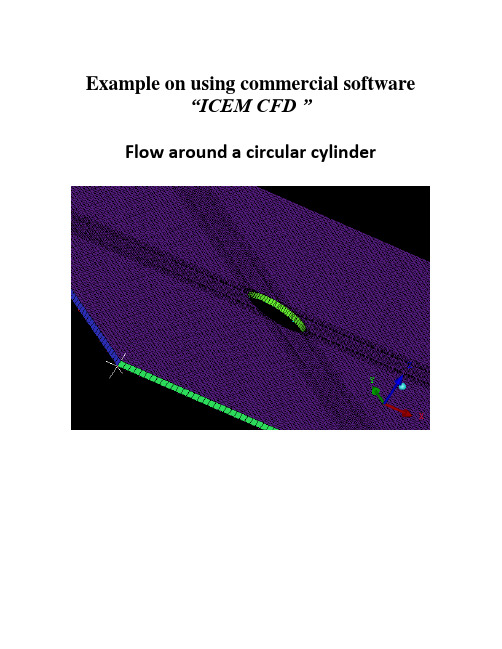
Example on using commercial software“ICEM CFD ”Flow around a circular cylinderTwo Dimensional problems；Flow around a circular cylinderProblem DescriptionAir flows across a cylinder with the uniform velocity s in the wind tunnel. The length of the wind tunnel (fluid domain) has 25m long and 10 m height. The diameter of cylinder is 1m .Assumption and Boundary Conditions: 1. 2 dimensional problems 2. Steady state condition 3. The uniform flow velocity 4. ！ 5. No Heat transfer6. Neglect the gravitational force7. Constant air densityPre-processing stageIn this stage, we implement the “ICEM CFD” to perform the pre-processing work. The basic steps as follow:1. Establish geometry model2. Block the parts3. Generation the O grid4. Mesh the model and check quality of mesh5. |6. Extrude the mesh7. Reset the BC’s (boundary conditions) 8. Output toCreating Geometry1. Open ICEM CFDOutle tDouble Click the “ICEM CFD” Icon, afterwards, you can see the interface of the ICEM CFD.，Open File>New Project…:Set the name with “cylinder_2d”, and Click “Save”!2. Creating Geometry:A.PointsClick button “Create Point”and then click button “Explicit Coordinates”Set the points in Cartesian coordinate system(X, Y, Z) with ( X=0, Y=0, Z=0 ) respectively. >Click “Apply” button and see the screen: a point is createdA tree widget can be seen at left of the screen (A) and (B)A B-The same method creates other points:X=0; Y=, X=-5; Y=5, -5X=20; Y=5, -5 Y=0; X=,：B.Draw line (curve)First of all see the tree widget, open Model>Geometry>Points by right buttonSelect Show Point Names and you can see the name ofeach point like the figure showed./Now you can create curvesClick button “Create/Modify Curve”!Click button “Create Curve”Note: the left corner of the black screen: Select locationswith left button, middle=done, right=cancelSelect points by using left button of the mouse.Change the name of the Part with “INLET”:A B&Select and with left button (A),And draw a line with middle button “done”(B) and the INLET part is created in the tree widget.The same steps draw the curves named “OUTLET, SIDEA, SIDEB” with the , and , and respectively.We will see the line and the tree widget|Draw the cylinderClick button“Circle or arc from Center point and 2 pointson plane”.Set the Part with name “CYLINDER”Click button and select points “, , ” with left buttonrespectively (A).*A BDraw the cylinder by middle button (B).~See tree widget:Close Points name Use button to fit the window.,Set the body and material.^Click button “Create Body”Choose button “Material Point”and select“Selected surfaces” in the “By Topology” menu.Change the name of the part with “FLUID”; open the ShowPoint Name of the tree widget and use selectand .The same way change the part name with “CYLINDER” and select and .Close Show Point Name and open the tree widget:￥Open the bodies and you can seeAt last, open the File>Geometry>Save Geometry As…Give it the name with “cylinder_2d”. Click “save”.,Now we begin to block the model.Click button “Create Block”See the first one , choose the part with “FLUID”,from the pull down menu select “FLUID”\And set the Initialize Blocks type with “2D Planar”Click “Apply” button.^A BWe will see that the colors of figure are changed. From (A) to (B)}See the tree widget: Model>BlockingThen create some assistant points with button “CreatePoint”、{Y=0X=,,,,,,,,, , , , , , , , , }{X=0Y=,,,,,,,,, , , , , , , , , }…Now begin to block the regionClick button “Split Block”Then select button “Split Block”{See the split method, select “Prescribed point”Use the put down menu to select the Prescribed point,、Use the button firstly select the Edge “INLET” andsecondly select the Point “”.We will see the block line in the vertical direction of theINLET.Zoom the fiure.The same way we draw other block lines.；From the “ to ”—See the tree widgetSelect the “Blocking” and select “Index Control”Model>Blocking: Index Control (using right button of the mouse) We can see at the right corner of the screen<By using button and we set I min=2 and see the figureThe same way we set I max =3 , J min=2 , J max=3 And the screen shown that，The same way block again from “, to ”:(A)(B)(C)After block.、See the tree widget: Model>Parts>VORFN :using the right button select “Add to Part”. Click button “Blocking Material”, Add Blocks to PartUsing select blocking regions and we can see！A B CZoom the block regions (A).Select the blocks in the cylinder or attached the cylinder (B)(C).Using the middle button to set it OK , and you can see blow (D).#Click button “Associate”）ABDCSelect the associate edge to curve “Associate Edge toCurve”button【Using the choose the edge and curveChoosing edge:]Select curves:]Set O grid CBAClick button “Split Block”Click “Ogird Block”button!Select theSee the tree widget: Open Model>Parts>VORFNOpen the VORFN (A)AUsing button to selectin or attached the cylinder (B)(C)(D).~B CUsing middle button to click “Apply” (E)Close “VORFN” from the tree widget (F)&DE"Click the “Reset”(G)!Mesh the edgesF GClick button “Set Curve Mesh Size”：Using button to select Curve(s):Choose Method with “Element count”Set the Number with 100 and click Apply.?）！See the tree: close the Model>Geometry>points, andthe Model>Blocking>edgesUsing right button to select Model>Geometry>Curves:Curve Node Spacing (by using right button)The same way set the “INLET” and “OUTLET” with number 100, the “SIDEA” and “SIDEB” with number 250.>Click button “Pre-Mesh Params”(Choose Blocking >Pre-Mesh Params;Click button “Update Sizes”and keep default,Then click Apply,See tree open Model>Blocking>Pre_Mesh: Project faces (by using right button) And we will see a menuClick Yes.'Now we will see the mesh of the model.Zoom it see the local partClose Geomery>Points and curves, and Blocking>Edges.^Then open File>Mesh>Load from BlockingOpen File>Mesh>Save Mesh As…: and set the name with “cylinder_2d”Open File>Blocking>Save Blocking As…: Save block with the name “cylinder_2d”Check the quality of the mesh￥Click button “Display Mesh Quality”Click Apply、We can see no negatives mesh."Extrude meshClick button “Extrude Mesh”Use to select Elements:$Method 1Click button “Select items in a part”and a menu appears:Click “All” and “Accept”Method 2 ，Put the left button and drag it to select all the regions (A)(C). Click middle button to accept (B)Give the New volume part name “FLUID2D”, new side part name “SIDE”, new top par name “TOP” And set the Spacing type>spacing with “”, then ApplySo the mesh change a height in the Z direction (D)AB-CBox Zoom …Click button “Shaded Full Display”(E)(F) Check the quality of the extrude mesh、DE FSee the tree widget:Close top “TOP” (B)Close “FLUID” (C) |：A BSet the new boundary conditions <See the tree widget:Model>Parts: Create Part (by using the right button)Click “Create Part by Selection” button From the pull down menu of the Part: select the “CYLINDER” Using and left button drag the regionUsing middle button accepts it, so a new CYLINDER boundary condition has been set (C).CBAC]The same way set the INLET, OUTLET, SIDEA and SIDEB boundary conditions. INLET:The Whole Boundary Conditions CA BSee the tree widget:?Open Model>Parts>FLUID(B)Open Model>Parts>TOP(C)B ASix kinds of patterns ]Click File>Mesh>Save Mesh As…<And save the new mesh with name“cylinder_2d_extrude”. Output the mesh file to CFXClick button “Select solver”and choose “CFX-5”CCBFEDAClick “Okay”)Click button “Write input”Keep default and click “Done”Then the Domain selection appearsKeep the Selected domains with “” and click “Done”.'Now we will see the created files in working directions:From these files, we must note that only the file named “cfx5” can be inputted intomesh is finished.Other examples:~Example on using commercial software “CFX around a circular cylinder'Two Dimensional problemsFlow around a circular cylinderAfter established the geometry model, we begin to use CFX to solve this two dimensional case.1.Processing with CFX~Double click the “CFX” Icon, afterwards, you can see the interface of the CFX.There are three kinds of functions of the CFX:1.CFX-Pre (set the relevant parameters).2.CFX-Solver (solve the case by using established physical model)3.CFX-Post (get the data and figures which we need)？CFX-Pre step:1.Import the mesh file from ICEM CFD2.Simulation type3.Domain4.BC’s (boundary conditions)5.Initial conditions6.Solver control7.Output file and monitor points8.Write “.def” file and simulation\Click button “CFX-Pre and run it.Establish a new simulationOpen File>New Simulation…:!Select button “General”and give the file name with“cylinder_2d”. Click “Save”Now we can see the interface of the CFX-Pre'Import mesh fileSee the middle position of the screen, Click button “Import mesh”>Open Mesh>Definition>Mesh Format:From the pull down menu select “ICEM CFD”, (see figure below)》Definition>File: Click button “Browse”Find the working direction and select the file named “cfx5”,《Then click “Open” button. And “OK”Note: no other files can be inputted in Then the mesh file has been inputted into the CFX-PreAnd the left window appears.…All of these names were already defined by us in “ICEM CFD”Set the relevant parameters1. Define the simulation type:Click button “Define the Simulation Type”button.~Note: the blue color note suggest we should set a domain.Then the simulation type appears！Basic Settings>Option: Select “Transient”/Basic Settings>Time Duration>Option: From the pull down menu select Total Time. Basic Settings>Time Duration>Total Time: Set with 42000s.Basic Settings>Time Steps>Option: From the pull down menu select Timesteps.Basic Settings>Time Steps>Timesteps: Set with 1s.Initial Time>Option: From the pull down menu select Autorratic.(Then click Apply and Ok2. Create a domain:Click button “Create a Domain”.Set the name with “ cylinder2d” and click Ok）See figure below: the color of the domain changed into green, and the window “Edit Domain”appears.General Options>Basic Settings>Location:From the pull down menu select“FLUID2D”；Then click“Apply” button、~Fluid Models>Heat Transfer Model>Option:Keep by default.Fluid Models>Heat Transfer Model>FluidTemperature: Set the temperature with 25c.Fluid Models>Turbulence Model>Option: Set itwith “None(Laminar).Click OK：3. Set boundary condtions:Click button “Create a Boundary Condition”Set INLET boundary conditionSet the Name with “INLET” and click OK：?Basic Settings>Boundary Type: From the pulldown menu select INLET.Boundary Details>Flow Regime>Option: SelectSubsonic.Boundary Details>Mass AndMomentum>Option: Select Normal Speed.Boundary Details>Mass AndMomentum>Normal Speed: Set it with m/sClick Ok:The right figure shows us that the INLET boundary condition has been set."Set OUTLET boundary condition。

试验十一流体分析

实验十一流体分析（一）实验目的1．熟悉并掌握ANSYS软件的使用方法；2．掌握如何利用ANSYS进行流体分析；（二）实验设备和工具安装有ANSYS软件的计算机（三）实验原理问题描述该算例是一个二维的导流管分析，先分析一个雷诺数为400的层流情况，然后改变流场参数再重新分析，最后再扩大分析区域来计算其湍流情况。

该算例所用单位制为国际单位制。

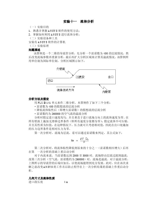
分析区域图示如下：分析方法及假定用FLUID141单元来作二维分析，本算例作了如下三个分析：·雷诺数为400的假想流的层流分析·降低流体粘性后（即增大雷诺数）的假想流的层流分析·雷诺数约为260000的空气流的湍流分析分析时假定进口速度均匀，并且垂直于进口流场方向上的流体速度为零。

在所有壁面上施加无滑移边界条件（即所有速度分量都为零）；假定流体不可压缩，并且其性质为恒值，在这种情况下，压力就可只考虑相对值，因此在出口处施加的压力边界条件是相对压力为零。

第一次分析时，流场为层流，着可以通过雷诺数来判定，其公式如下：进口段高度 1 m过渡段长度 2 m出口段高度 2.5 m层流分析时出口段长度 6 m湍流分析时出口段长度12 m假设流体密度 1 Kg/m3假设流体粘性第一次分析0.01Kg/m-s；第二次分析0.001 Kg/m-s 空气密度 1.205 Kg/m3空气粘性 1.8135*10-5 Kg/m-s进口速度 2.0 m/s出口压力0 nt/m2（四）实验步骤第1步：进入ANSYS第2步：设置分析选择1 进入Main Menu>Preference2 点取FLOTRAN CFD项3 点取OK第3步：定义单元类型1 进入Main Menu>Preprocessor>Element Type>Add/Edit/Delete2 点取Add3 在弹出菜单的左框中点取FLOTRAN CFD，右框中点取2D FLOTRAN 1414 点取OK5 点取Close第4步：生成分析区域的几何面该步定义三个面：分别表示进口和出口的两个矩形面，以及一个表示过渡段的面。

1、下载文档前请自行甄别文档内容的完整性，平台不提供额外的编辑、内容补充、找答案等附加服务。
2、"仅部分预览"的文档,不可在线预览部分如存在完整性等问题,可反馈申请退款(可完整预览的文档不适用该条件!)。
3、如文档侵犯您的权益，请联系客服反馈,我们会尽快为您处理(人工客服工作时间：9:00-18:30)。

ANSYS CFD管道流体分析算例Fluid11

ansys fluent中文版流体计算工程案例详解

ANSYS流体第4章flotran流体分析典型工程实例

ANSYS教学算例集FL_工艺注射混合管流场分析

ANSYS／FLOTRAN流体动力学(CFD)分析

ANSYS／FLOTRAN流体动力学CFD分析

最新ANSYS-CFD之Flotran中文讲解说明(全+重点标注)11资料

ANSYS流体分析

最新ANSYS-CFD之Flotran中文讲解说明（全+重点标注）11资料

ANSYS CFD管道流体分析算例Fluid11

ANSYS流体第4节flotran流体分析典型工程实例

ansys cfd入门指南计算流体力学基础与应用

ANSYS模拟风荷载流体力学计算

ansys流体分析FLOTRAN

ansys-fluids流体计算的例子

ansys help流固耦合算例fluid_structure(内含解析)

ansys_cfd流体分析实例

试验十一流体分析