A Linear Algorithm for Tracing Magnet Position and Orientation by Using Three-Axis Magnetic Sensors
写出光线跟踪递归函数的伪代码。

写出光线跟踪递归函数的伪代码。
光线跟踪是一种计算机图形学中常用的方法,用于模拟物体表面反射光线的行为,从而生成逼真的图像。
下面是光线跟踪递归函数的伪代码:```pythonRay Trace(Point3D origin, Vector3D direction, int depth):if depth == MAX_DEPTH: # 达到递归深度,结束递归return BACKGROUND_COLOR# 找到离射线最近的交点hit_distance, hit_point, hit_norm, hit_obj = findIntersection(origin, direction)if not hit_obj: # 未与任何物体相交,返回背景颜色return BACKGROUND_COLOR# 计算环境光照color = hit_obj.material.ambient_color * AMBIENT_LIGHT_COLOR# 计算入射光照for light in scene.lights:light_direction = normalize(light.position - hit_point)# 检查是否有阴影if not isShadowed(hit_point, light.position, hit_obj):color += computeDiffuseColor(hit_obj.material.diffuse_color, light.color, light_direction, hit_norm)color += computeSpecularColor(hit_obj.material.specular_color, light.color, light_direction, hit_norm, direction)前两个参数是光线的起点和方向向量,第三个参数是当前递归深度。
Linear Programming for Optimization
1 .1 Definition Linear programming is the name of a branch of applied mathematics that deals with solving optimization problems of a particular form. Linear programming problems consist of a linear cost function (consisting of a certain number of variables) which is to be minimized or maximized subject to a certain number of constraints. The constraints are linear inequalities of the variables used in the cost function. The cost function is also sometimes called the objective function. Linear programming is closely related to linear algebra; the most noticeable difference is that linear programming often uses inequalities in the problem statement rather than equalities. 1 .2 History Linear programming is a relatively young mathematical discipline, dating from the invention of the simplex method by G. B. Dantzig in 1947. Historically, development in linear programming is driven by its applications in economics and management. Dantzig initially developed the simplex method to solve U.S. Air Force planning problems, and planning and scheduling problems still dominate the applications of linear programming. One reason that linear programming is a relatively new field is that only the smallest linear programming problems can be solved without a computer. 1 .3 Example (Adapted from [1].) Linear programming problems arise naturally in production planning. Suppose a particular Ford plant can build Escorts at the rate of one per minute, Explorer at the rate of one every 2 minutes, and Lincoln Navigators at the rate of one every 3 minutes. The vehicles get 25, 15, and 10 miles per gallon, respectively, and Congress mandates that the average fuel economy of vehicles produced be at least 18 miles per gallon. Ford loses $1000 on each Escort, but makes a profit of $5000 on each Explorer and $15,000 on each Navigator. What is the maximum profit this Ford plant can make in one 8-hour day?
Synopsys OptoDesigner 2020.09安装指南说明书
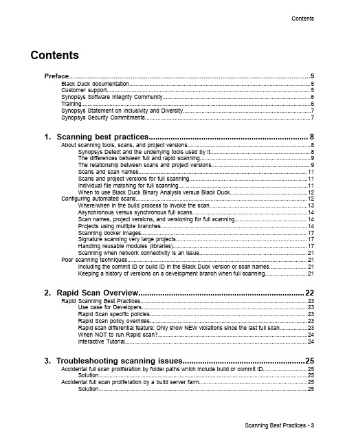
3. Troubleshooting scanning issues........................................................25
Accidental full scan proliferation by folder paths which include build or commit ID............................ 25 Solution......................................................................................................................................25
Contents
Contents
Preface....................................................................................................5
1. Scanning best practices......................................................................... 8
A_star算法
Amit's A star Page中译文译序这篇文章很适合A*算法的初学者,可惜网上没找到翻译版的。
本着好东西不敢独享的想法,也为了锻炼一下英文,本人译了这篇文章。
由于本人英文水平非常有限,六级考了两次加一块不超过370分,因此本译文难免存在问题。
不过也算是抛砖引玉,希望看到有更多的游戏开发方面的优秀译作出现,毕竟中文的优秀资料太少了,中国的游戏开发者的路不好走。
本人能力有限,译文中有小部分词句实在难以翻译,因此暂时保留英文原文放在译文中。
对于不敢确定翻译是否准确的词句,本人用圆括号保留了英文原文,读者可以对照着加以理解。
A*算法本身是很简单的,因此原文中并没有过多地讨论A*算法本身,而是花了较大的篇幅讨论了用于保存OPEN和CLOSED集的数据结构,以及A*算法的变种和扩展。
编程实现A*是简单的,读者可以用STL对本文中的伪代码加以实现(本人已花一天时间实验过基本的A*搜索)。
但是最重要的还是对A*本身的理解,这样才可以在自己的游戏中处理各种千变万化的情况。
翻译本文的想法产生于2006年5月,实际完成于2007年4月到6月,非常惭愧。
最后,本译文仅供交流和参考,对于因本译文放到网上而产生的任何问题,本人不负任何责任。
蔡鸿于南开大学软件学院2007年6月9日原文地址:/~amitp/GameProgramming/相关链接:/%7Eamitp/gameprog.html#Paths我们尝试解决的问题是把一个游戏对象(game object)从出发点移动到目的地。
路径搜索(Pathfinding)的目标是找到一条好的路径——避免障碍物、敌人,并把代价(燃料,时间,距离,装备,金钱等)最小化。
运动(Movement)的目标是找到一条路径并且沿着它行进。
把关注的焦点仅集中于其中的一种方法是可能的。
一种极端情况是,当游戏对象开始移动时,一个老练的路径搜索器(pathfinder)外加一个琐细的运动算法(movement algorithm)可以找到一条路径,游戏对象将会沿着该路径移动而忽略其它的一切。
1-s2.0-S0024379513004217-main

Contents lists available at SciVerse ScienceDirect
Linear Algebra and its Applications
/locate/laa
where i = 1, . . . , n. Then we have |x| = T z x, where z = sign x ∈ Y n . For a given interval matrix A = [ A c − A , A c + A ] ∈ IRm×n , and for each vector y ∈ Y m and each vector z ∈ Y n , we introduce the matrices
m
b
b ,
where b, b ∈ R , and b b . The set of all m-by-n interval matrices will be denoted by IRm×n and the set of all m-dimensional interval vectors by IRm . Denote by A c and A the center and radius matrices given by
Ac =
1 2 1 2
( A + A ),
A
= ( A − A ),
2
1
respectively. Then A = [ A c − A , A c + A ]. Similarly, the center and radius vectors are defined as
LTE无线网络多频段弱信号快速捕捉算法

第37卷第12期计算机仿真2020年12月文章编号:1006 -9348(2020) 12 -0144 -04L T E无线网络多频段弱信号快速捕捉算法钟文华,刘成国(武汉理工大学理学院,湖北武汉430070)摘要:由于传统LTE无线网络多频段弱信号捕捉算法的运算量大,计算较为复杂,不能实现对弱信号的快速、精准捕捉。
因此提出LTE无线网络多频段弱信号快速捕捉算法。
通过构建LTE无线网络通信系统模型,确定系统稳定运行的必要条件,利用可靠性函数计算系统成功服务概率;根据计算结果,结合FFT快速捕捉算法的基本原理,对LTE无线网络通信信号做 正交与积分处理,采用差分相干算法去除运算损耗,从而捕捉到LTE无线网络通信系统中多频段弱信号的载波频率,并对 其做精化处理,从而达到LTE无线网络多频段弱信号快速捕捉的目的。
仿真结果证明,所提算法在相同的无线网络通信环 境下具有更高的捕捉效率,且捕捉精度远远高于其他方法。
关键词:弱信号;快速捕捉;分段叠加中图分类号:TP914 文献标识码:BFast Multi Band W e a k Signal AcquisitionAlgorithm in L T E Wireless NetworkZHONG Wen - hua,LIU Cheng - guo(Wuhan University of Technology School of Science,Hubei Wuhan430070, China)A B S T R A C T:Due to the large amount of computation and complexity in traditional algorithms,it is unable to achievefast and accurate acquisition for weak signals.Therefore,an algorithm of fast acquisition for multi- band weak signal in LTE wireless network was put forward.Firstly,the model of LTE wireless network communication system was used to determine the necessary conditions for stable operation of system,and then the reliability function was used to calculate the probability of successful service of system.According to the calculation results and the basic principle of FFT fast capture algorithm,the orthogonal and integral processing was performed on LTE wireless network communication signal,and the difference coherence algorithm was used to remove the computing loss,so as to capture the carrier frequency of multi- band weak signal in LTE wireless network communication.Finally,the carrier frequency was refined to achieve the fast acquisition of multi- band weak signal in LTE wireless network.Simulation results show that the proposed algorithm has higher capture efficiency in the same wireless network communication environment, and the capture accuracy is much higher than other methods.K E Y W O R D S:Weak signal;Fast capture;Piecewise superpositioni引言L T E为第四代移动通信的主要技术,随着业务应用范围 的不断扩大,应用类型也随之增多。
数学名词及其简单介绍
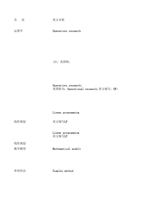
名 词英文名称运筹学Operations research(注:美国称:Operations research;英国称为:Operational research;英文缩写:OR)Linear programming线性规划英文缩写LPLinear programming英文缩写LP线性规划数学模型Mathematical models单纯形法Simplex methodSimplex method单纯形法改进单纯形法Revised Simplex method目标函数Objective约束条件Constraints可行解Feasible solutions可行域Feasible region名 词英文名称线性规划图解法Graphical Solution of Linear Programs对偶理论Duality theory对偶单纯Dual Simplex method形法影子价格Shadow price运输问题transportation problemtransportation problem运输问题目标规划法Goal programming表上作业法Tabular method表上作业法Tabular method图上作业法Graphical method灵敏度分析Sensitivity analysis西北角法Northwest corner rule名 词英文名称最小元素The least cost rule法运输论法Transportation闭回路调整法Close circular adjust method名 词英文名称非线性规划Nonlinear programming斐波那契法Fibonacci search0.618法Golden section search(黄金分割法)欧拉回路Euler loop整数规划Integer programming松弛问题Slack problem名 词英文名称割平面法Cutting plane method分枝限界Branch and bound method法整数线性规划Integer linear programming纯整数线性规划Pure Integer linear programming名 词英文名称混合整数Mixed Integer linear prog.线性规划0-1型整数线性规划Zero-one Integer linear programming 隐枚举法Implicit Enumeration马氏决策Markov decision programming规划最小树问Minimal tree problem题名 词英文名称最短路问Shortest-route problems题Dijkstra算法Dijkstra algorithmFloyd算法Floyd algorithm最大流问Maximal-Flow problems题图与网络分析Graph theory and network analysis 网络计划Network program网络Network网络方法Network method and network planning 和网络计划网络分析Network analysis网络技术Network techniques名 词英文名称关键线路Critical path method 简称CPM法计划评审Program eval-法uation & rev-iew technique简称PERT网络图Network graphic多重图和Multiple graph and简单图simple graph连通图Connected graph无向图Non-oriented graph有向图oriented graph名 词英文名称最短路径问题Shortest path problem动态规划Dynamic programming缩写DP决策Decision决策论Decision theory名 词英文名称现代决策Modern decision theory理论古典决策Classical decision theory理论战略决策Strategy decision风险型决Risk decision策益损矩阵Opportunity loss matrix最大可能Maximal probability criterion法名 词英文名称期望值法Expected value method决策树法Decision trees method局中人Player策略Policy马氏决策Markov decision programming规划英文缩写:MDP悲观准则Max-min criterion(max-min准则)乐观准则Max-max criterion名 词英文名称折衷准则Trade-off criterion等可能准则(Laplace准则)Laplace criterion遗憾准则(min-max准则)Regret criterion对策论Game theory合作对策Cooperative games名 词英文名称非合作对Non-cooperative games 策纳什平衡Nash equilibrium帕雷托最Pareto optimality优斯塔克尔贝格对策Stackelberg strategy统筹法Overall planning method 指派问题Assignment problem匈牙利解Hungarian method法存储论Inventory theory排队论Queuing theory名 词英文名称排队系统Queuing system生灭过程Birth-death process支付矩阵The payoffmatrix内 容运筹学是一门运用于管理有组织系统的科学。
Indradrive 系列 故障代码

Error MessagesF9001 Error internal function call.F9002 Error internal RTOS function callF9003 WatchdogF9004 Hardware trapF8000 Fatal hardware errorF8010 Autom. commutation: Max. motion range when moving back F8011 Commutation offset could not be determinedF8012 Autom. commutation: Max. motion rangeF8013 Automatic commutation: Current too lowF8014 Automatic commutation: OvercurrentF8015 Automatic commutation: TimeoutF8016 Automatic commutation: Iteration without resultF8017 Automatic commutation: Incorrect commutation adjustment F8018 Device overtemperature shutdownF8022 Enc. 1: Enc. signals incorr. (can be cleared in ph. 2) F8023 Error mechanical link of encoder or motor connectionF8025 Overvoltage in power sectionF8027 Safe torque off while drive enabledF8028 Overcurrent in power sectionF8030 Safe stop 1 while drive enabledF8042 Encoder 2 error: Signal amplitude incorrectF8057 Device overload shutdownF8060 Overcurrent in power sectionF8064 Interruption of motor phaseF8067 Synchronization PWM-Timer wrongF8069 +/-15Volt DC errorF8070 +24Volt DC errorF8076 Error in error angle loopF8078 Speed loop error.F8079 Velocity limit value exceededF8091 Power section defectiveF8100 Error when initializing the parameter handlingF8102 Error when initializing power sectionF8118 Invalid power section/firmware combinationF8120 Invalid control section/firmware combinationF8122 Control section defectiveF8129 Incorrect optional module firmwareF8130 Firmware of option 2 of safety technology defectiveF8133 Error when checking interrupting circuitsF8134 SBS: Fatal errorF8135 SMD: Velocity exceededF8140 Fatal CCD error.F8201 Safety command for basic initialization incorrectF8203 Safety technology configuration parameter invalidF8813 Connection error mains chokeF8830 Power section errorF8838 Overcurrent external braking resistorF7010 Safely-limited increment exceededF7011 Safely-monitored position, exceeded in pos. DirectionF7012 Safely-monitored position, exceeded in neg. DirectionF7013 Safely-limited speed exceededF7020 Safe maximum speed exceededF7021 Safely-limited position exceededF7030 Position window Safe stop 2 exceededF7031 Incorrect direction of motionF7040 Validation error parameterized - effective thresholdF7041 Actual position value validation errorF7042 Validation error of safe operation modeF7043 Error of output stage interlockF7050 Time for stopping process exceeded8.3.15 F7051 Safely-monitored deceleration exceeded (159)8.4 Travel Range Errors (F6xxx) (161)8.4.1 Behavior in the Case of Travel Range Errors (161)8.4.2 F6010 PLC Runtime Error (162)8.4.3 F6024 Maximum braking time exceeded (163)8.4.4 F6028 Position limit value exceeded (overflow) (164)8.4.5 F6029 Positive position limit exceeded (164)8.4.6 F6030 Negative position limit exceeded (165)8.4.7 F6034 Emergency-Stop (166)8.4.8 F6042 Both travel range limit switches activated (167)8.4.9 F6043 Positive travel range limit switch activated (167)8.4.10 F6044 Negative travel range limit switch activated (168)8.4.11 F6140 CCD slave error (emergency halt) (169)8.5 Interface Errors (F4xxx) (169)8.5.1 Behavior in the Case of Interface Errors (169)8.5.2 F4001 Sync telegram failure (170)8.5.3 F4002 RTD telegram failure (171)8.5.4 F4003 Invalid communication phase shutdown (172)8.5.5 F4004 Error during phase progression (172)8.5.6 F4005 Error during phase regression (173)8.5.7 F4006 Phase switching without ready signal (173)8.5.8 F4009 Bus failure (173)8.5.9 F4012 Incorrect I/O length (175)8.5.10 F4016 PLC double real-time channel failure (176)8.5.11 F4017 S-III: Incorrect sequence during phase switch (176)8.5.12 F4034 Emergency-Stop (177)8.5.13 F4140 CCD communication error (178)8.6 Non-Fatal Safety Technology Errors (F3xxx) (178)8.6.1 Behavior in the Case of Non-Fatal Safety Technology Errors (178)8.6.2 F3111 Refer. missing when selecting safety related end pos (179)8.6.3 F3112 Safe reference missing (179)8.6.4 F3115 Brake check time interval exceeded (181)Troubleshooting Guide | Rexroth IndraDrive Electric Drivesand ControlsI Bosch Rexroth AG VII/XXIITable of ContentsPage8.6.5 F3116 Nominal load torque of holding system exceeded (182)8.6.6 F3117 Actual position values validation error (182)8.6.7 F3122 SBS: System error (183)8.6.8 F3123 SBS: Brake check missing (184)8.6.9 F3130 Error when checking input signals (185)8.6.10 F3131 Error when checking acknowledgment signal (185)8.6.11 F3132 Error when checking diagnostic output signal (186)8.6.12 F3133 Error when checking interrupting circuits (187)8.6.13 F3134 Dynamization time interval incorrect (188)8.6.14 F3135 Dynamization pulse width incorrect (189)8.6.15 F3140 Safety parameters validation error (192)8.6.16 F3141 Selection validation error (192)8.6.17 F3142 Activation time of enabling control exceeded (193)8.6.18 F3143 Safety command for clearing errors incorrect (194)8.6.19 F3144 Incorrect safety configuration (195)8.6.20 F3145 Error when unlocking the safety door (196)8.6.21 F3146 System error channel 2 (197)8.6.22 F3147 System error channel 1 (198)8.6.23 F3150 Safety command for system start incorrect (199)8.6.24 F3151 Safety command for system halt incorrect (200)8.6.25 F3152 Incorrect backup of safety technology data (201)8.6.26 F3160 Communication error of safe communication (202)8.7 Non-Fatal Errors (F2xxx) (202)8.7.1 Behavior in the Case of Non-Fatal Errors (202)8.7.2 F2002 Encoder assignment not allowed for synchronization (203)8.7.3 F2003 Motion step skipped (203)8.7.4 F2004 Error in MotionProfile (204)8.7.5 F2005 Cam table invalid (205)8.7.6 F2006 MMC was removed (206)8.7.7 F2007 Switching to non-initialized operation mode (206)8.7.8 F2008 RL The motor type has changed (207)8.7.9 F2009 PL Load parameter default values (208)8.7.10 F2010 Error when initializing digital I/O (-> S-0-0423) (209)8.7.11 F2011 PLC - Error no. 1 (210)8.7.12 F2012 PLC - Error no. 2 (210)8.7.13 F2013 PLC - Error no. 3 (211)8.7.14 F2014 PLC - Error no. 4 (211)8.7.15 F2018 Device overtemperature shutdown (211)8.7.16 F2019 Motor overtemperature shutdown (212)8.7.17 F2021 Motor temperature monitor defective (213)8.7.18 F2022 Device temperature monitor defective (214)8.7.19 F2025 Drive not ready for control (214)8.7.20 F2026 Undervoltage in power section (215)8.7.21 F2027 Excessive oscillation in DC bus (216)8.7.22 F2028 Excessive deviation (216)8.7.23 F2031 Encoder 1 error: Signal amplitude incorrect (217)VIII/XXII Bosch Rexroth AG | Electric Drivesand ControlsRexroth IndraDrive | Troubleshooting GuideTable of ContentsPage8.7.24 F2032 Validation error during commutation fine adjustment (217)8.7.25 F2033 External power supply X10 error (218)8.7.26 F2036 Excessive position feedback difference (219)8.7.27 F2037 Excessive position command difference (220)8.7.28 F2039 Maximum acceleration exceeded (220)8.7.29 F2040 Device overtemperature 2 shutdown (221)8.7.30 F2042 Encoder 2: Encoder signals incorrect (222)8.7.31 F2043 Measuring encoder: Encoder signals incorrect (222)8.7.32 F2044 External power supply X15 error (223)8.7.33 F2048 Low battery voltage (224)8.7.34 F2050 Overflow of target position preset memory (225)8.7.35 F2051 No sequential block in target position preset memory (225)8.7.36 F2053 Incr. encoder emulator: Pulse frequency too high (226)8.7.37 F2054 Incr. encoder emulator: Hardware error (226)8.7.38 F2055 External power supply dig. I/O error (227)8.7.39 F2057 Target position out of travel range (227)8.7.40 F2058 Internal overflow by positioning input (228)8.7.41 F2059 Incorrect command value direction when positioning (229)8.7.42 F2063 Internal overflow master axis generator (230)8.7.43 F2064 Incorrect cmd value direction master axis generator (230)8.7.44 F2067 Synchronization to master communication incorrect (231)8.7.45 F2068 Brake error (231)8.7.46 F2069 Error when releasing the motor holding brake (232)8.7.47 F2074 Actual pos. value 1 outside absolute encoder window (232)8.7.48 F2075 Actual pos. value 2 outside absolute encoder window (233)8.7.49 F2076 Actual pos. value 3 outside absolute encoder window (234)8.7.50 F2077 Current measurement trim wrong (235)8.7.51 F2086 Error supply module (236)8.7.52 F2087 Module group communication error (236)8.7.53 F2100 Incorrect access to command value memory (237)8.7.54 F2101 It was impossible to address MMC (237)8.7.55 F2102 It was impossible to address I2C memory (238)8.7.56 F2103 It was impossible to address EnDat memory (238)8.7.57 F2104 Commutation offset invalid (239)8.7.58 F2105 It was impossible to address Hiperface memory (239)8.7.59 F2110 Error in non-cyclical data communic. of power section (240)8.7.60 F2120 MMC: Defective or missing, replace (240)8.7.61 F2121 MMC: Incorrect data or file, create correctly (241)8.7.62 F2122 MMC: Incorrect IBF file, correct it (241)8.7.63 F2123 Retain data backup impossible (242)8.7.64 F2124 MMC: Saving too slowly, replace (243)8.7.65 F2130 Error comfort control panel (243)8.7.66 F2140 CCD slave error (243)8.7.67 F2150 MLD motion function block error (244)8.7.68 F2174 Loss of motor encoder reference (244)8.7.69 F2175 Loss of optional encoder reference (245)Troubleshooting Guide | Rexroth IndraDrive Electric Drivesand Controls| Bosch Rexroth AG IX/XXIITable of ContentsPage8.7.70 F2176 Loss of measuring encoder reference (246)8.7.71 F2177 Modulo limitation error of motor encoder (246)8.7.72 F2178 Modulo limitation error of optional encoder (247)8.7.73 F2179 Modulo limitation error of measuring encoder (247)8.7.74 F2190 Incorrect Ethernet configuration (248)8.7.75 F2260 Command current limit shutoff (249)8.7.76 F2270 Analog input 1 or 2, wire break (249)8.7.77 F2802 PLL is not synchronized (250)8.7.78 F2814 Undervoltage in mains (250)8.7.79 F2815 Overvoltage in mains (251)8.7.80 F2816 Softstart fault power supply unit (251)8.7.81 F2817 Overvoltage in power section (251)8.7.82 F2818 Phase failure (252)8.7.83 F2819 Mains failure (253)8.7.84 F2820 Braking resistor overload (253)8.7.85 F2821 Error in control of braking resistor (254)8.7.86 F2825 Switch-on threshold braking resistor too low (255)8.7.87 F2833 Ground fault in motor line (255)8.7.88 F2834 Contactor control error (256)8.7.89 F2835 Mains contactor wiring error (256)8.7.90 F2836 DC bus balancing monitor error (257)8.7.91 F2837 Contactor monitoring error (257)8.7.92 F2840 Error supply shutdown (257)8.7.93 F2860 Overcurrent in mains-side power section (258)8.7.94 F2890 Invalid device code (259)8.7.95 F2891 Incorrect interrupt timing (259)8.7.96 F2892 Hardware variant not supported (259)8.8 SERCOS Error Codes / Error Messages of Serial Communication (259)9 Warnings (Exxxx) (263)9.1 Fatal Warnings (E8xxx) (263)9.1.1 Behavior in the Case of Fatal Warnings (263)9.1.2 E8025 Overvoltage in power section (263)9.1.3 E8026 Undervoltage in power section (264)9.1.4 E8027 Safe torque off while drive enabled (265)9.1.5 E8028 Overcurrent in power section (265)9.1.6 E8029 Positive position limit exceeded (266)9.1.7 E8030 Negative position limit exceeded (267)9.1.8 E8034 Emergency-Stop (268)9.1.9 E8040 Torque/force actual value limit active (268)9.1.10 E8041 Current limit active (269)9.1.11 E8042 Both travel range limit switches activated (269)9.1.12 E8043 Positive travel range limit switch activated (270)9.1.13 E8044 Negative travel range limit switch activated (271)9.1.14 E8055 Motor overload, current limit active (271)9.1.15 E8057 Device overload, current limit active (272)X/XXII Bosch Rexroth AG | Electric Drivesand ControlsRexroth IndraDrive | Troubleshooting GuideTable of ContentsPage9.1.16 E8058 Drive system not ready for operation (273)9.1.17 E8260 Torque/force command value limit active (273)9.1.18 E8802 PLL is not synchronized (274)9.1.19 E8814 Undervoltage in mains (275)9.1.20 E8815 Overvoltage in mains (275)9.1.21 E8818 Phase failure (276)9.1.22 E8819 Mains failure (276)9.2 Warnings of Category E4xxx (277)9.2.1 E4001 Double MST failure shutdown (277)9.2.2 E4002 Double MDT failure shutdown (278)9.2.3 E4005 No command value input via master communication (279)9.2.4 E4007 SERCOS III: Consumer connection failed (280)9.2.5 E4008 Invalid addressing command value data container A (280)9.2.6 E4009 Invalid addressing actual value data container A (281)9.2.7 E4010 Slave not scanned or address 0 (281)9.2.8 E4012 Maximum number of CCD slaves exceeded (282)9.2.9 E4013 Incorrect CCD addressing (282)9.2.10 E4014 Incorrect phase switch of CCD slaves (283)9.3 Possible Warnings When Operating Safety Technology (E3xxx) (283)9.3.1 Behavior in Case a Safety Technology Warning Occurs (283)9.3.2 E3100 Error when checking input signals (284)9.3.3 E3101 Error when checking acknowledgment signal (284)9.3.4 E3102 Actual position values validation error (285)9.3.5 E3103 Dynamization failed (285)9.3.6 E3104 Safety parameters validation error (286)9.3.7 E3105 Validation error of safe operation mode (286)9.3.8 E3106 System error safety technology (287)9.3.9 E3107 Safe reference missing (287)9.3.10 E3108 Safely-monitored deceleration exceeded (288)9.3.11 E3110 Time interval of forced dynamization exceeded (289)9.3.12 E3115 Prewarning, end of brake check time interval (289)9.3.13 E3116 Nominal load torque of holding system reached (290)9.4 Non-Fatal Warnings (E2xxx) (290)9.4.1 Behavior in Case a Non-Fatal Warning Occurs (290)9.4.2 E2010 Position control with encoder 2 not possible (291)9.4.3 E2011 PLC - Warning no. 1 (291)9.4.4 E2012 PLC - Warning no. 2 (291)9.4.5 E2013 PLC - Warning no. 3 (292)9.4.6 E2014 PLC - Warning no. 4 (292)9.4.7 E2021 Motor temperature outside of measuring range (292)9.4.8 E2026 Undervoltage in power section (293)9.4.9 E2040 Device overtemperature 2 prewarning (294)9.4.10 E2047 Interpolation velocity = 0 (294)9.4.11 E2048 Interpolation acceleration = 0 (295)9.4.12 E2049 Positioning velocity >= limit value (296)9.4.13 E2050 Device overtemp. Prewarning (297)Troubleshooting Guide | Rexroth IndraDrive Electric Drivesand Controls| Bosch Rexroth AG XI/XXIITable of ContentsPage9.4.14 E2051 Motor overtemp. prewarning (298)9.4.15 E2053 Target position out of travel range (298)9.4.16 E2054 Not homed (300)9.4.17 E2055 Feedrate override S-0-0108 = 0 (300)9.4.18 E2056 Torque limit = 0 (301)9.4.19 E2058 Selected positioning block has not been programmed (302)9.4.20 E2059 Velocity command value limit active (302)9.4.21 E2061 Device overload prewarning (303)9.4.22 E2063 Velocity command value > limit value (304)9.4.23 E2064 Target position out of num. range (304)9.4.24 E2069 Holding brake torque too low (305)9.4.25 E2070 Acceleration limit active (306)9.4.26 E2074 Encoder 1: Encoder signals disturbed (306)9.4.27 E2075 Encoder 2: Encoder signals disturbed (307)9.4.28 E2076 Measuring encoder: Encoder signals disturbed (308)9.4.29 E2077 Absolute encoder monitoring, motor encoder (encoder alarm) (308)9.4.30 E2078 Absolute encoder monitoring, opt. encoder (encoder alarm) (309)9.4.31 E2079 Absolute enc. monitoring, measuring encoder (encoder alarm) (309)9.4.32 E2086 Prewarning supply module overload (310)9.4.33 E2092 Internal synchronization defective (310)9.4.34 E2100 Positioning velocity of master axis generator too high (311)9.4.35 E2101 Acceleration of master axis generator is zero (312)9.4.36 E2140 CCD error at node (312)9.4.37 E2270 Analog input 1 or 2, wire break (312)9.4.38 E2802 HW control of braking resistor (313)9.4.39 E2810 Drive system not ready for operation (314)9.4.40 E2814 Undervoltage in mains (314)9.4.41 E2816 Undervoltage in power section (314)9.4.42 E2818 Phase failure (315)9.4.43 E2819 Mains failure (315)9.4.44 E2820 Braking resistor overload prewarning (316)9.4.45 E2829 Not ready for power on (316)。
中国科学院深圳先进技术研究院导师简况表导师姓名孟庆虎性别男
Direction
biomedical engineering, medical robotics, interactive tele-medicine and tele-healthcare, bio-sensors and multi-sensor data fusion, bioinformatics and adaptive and intelligent systems, computervision.
研究方向
生物医学工程、医用机器人、交互式远程医疗、生物传感器、生物信息学和自适应智能系统、计算机视觉等
在研课题
中科院知识创新工程—“骨科手术机器人”
国家(科技部)科技支撑计划-“面向乡镇卫生院的多功能一体化体检设备”
广东省/中科院院地合作项目-“新型胶囊内窥镜”
个人简历
1988年获北京理工大学硕士学位,1992年于加拿大维多利亚大学电气及计算机工程系获博士学位。同年受聘到加拿大莱克海德大学任助理教授。1994年受聘转任加拿大阿尔伯塔大学电气及计算机工程系助理教授和高级机器人及遥控研究室主任,1998年提升为副教授并转为终身教授,2000年提升为正教授。2001年任香港中文大学自动化与计算机辅助工程系访问教授,2002年起任香港中文大学电子工程系教授。2006年起任深圳先进技术研究院研究员。
纹理物体缺陷的视觉检测算法研究--优秀毕业论文
摘 要
在竞争激烈的工业自动化生产过程中,机器视觉对产品质量的把关起着举足 轻重的作用,机器视觉在缺陷检测技术方面的应用也逐渐普遍起来。与常规的检 测技术相比,自动化的视觉检测系统更加经济、快捷、高效与 安全。纹理物体在 工业生产中广泛存在,像用于半导体装配和封装底板和发光二极管,现代 化电子 系统中的印制电路板,以及纺织行业中的布匹和织物等都可认为是含有纹理特征 的物体。本论文主要致力于纹理物体的缺陷检测技术研究,为纹理物体的自动化 检测提供高效而可靠的检测算法。 纹理是描述图像内容的重要特征,纹理分析也已经被成功的应用与纹理分割 和纹理分类当中。本研究提出了一种基于纹理分析技术和参考比较方式的缺陷检 测算法。这种算法能容忍物体变形引起的图像配准误差,对纹理的影响也具有鲁 棒性。本算法旨在为检测出的缺陷区域提供丰富而重要的物理意义,如缺陷区域 的大小、形状、亮度对比度及空间分布等。同时,在参考图像可行的情况下,本 算法可用于同质纹理物体和非同质纹理物体的检测,对非纹理物体 的检测也可取 得不错的效果。 在整个检测过程中,我们采用了可调控金字塔的纹理分析和重构技术。与传 统的小波纹理分析技术不同,我们在小波域中加入处理物体变形和纹理影响的容 忍度控制算法,来实现容忍物体变形和对纹理影响鲁棒的目的。最后可调控金字 塔的重构保证了缺陷区域物理意义恢复的准确性。实验阶段,我们检测了一系列 具有实际应用价值的图像。实验结果表明 本文提出的纹理物体缺陷检测算法具有 高效性和易于实现性。 关键字: 缺陷检测;纹理;物体变形;可调控金字塔;重构
Keywords: defect detection, texture, object distortion, steerable pyramid, reconstruction
II
a星算法融合dwa算法的代码
a星算法融合dwa算法的代码要融合A*算法和DWA算法,需要在A*算法的基础上添加DWA算法的部分。
A*算法用于路径规划,基于启发式函数和代价函数,能够找到最优路径。
而DWA算法用于运动控制,基于机器人当前状态和环境信息,通过调整机器人的速度和方向来避开障碍物。
以下是一个简单的实现示例,假设有一个二维平面上的机器人进行路径规划和运动控制:```pythonimport mathimport heapq#定义机器人的状态类class RobotState:def __init__(self, x, y, theta):self.x = xself.y = yself.theta = theta#定义A*算法中的节点类class Node:def __init__(self, state, g, h, parent=None):self.state = stateself.g = gself.h = hself.f = g + hself.parent = parent#用于比较节点的优先级def __lt__(self, other):return self.f < other.f#定义启发式函数,计算当前节点到目标节点的代价估计def heuristic_cost(node, goal):dx = node.state.x - goal.xdy = node.state.y - goal.yreturn math.sqrt(dx*dx + dy*dy)#定义代价函数,通过计算机器人当前状态和运动控制的代价def cost_function(current_state, control):#根据机器人的运动学模型来计算代价#...return cost#A*算法def astar_planner(start, goal, controls, obstacles):open_set = []closed_set = setheapq.heappush(open_set, Node(start, 0, heuristic_cost(start, goal)))while open_set:current_node = heapq.heappop(open_set)current_state = current_node.stateif current_state == goal:path = []current = current_nodewhile current is not None:path.append(current.state)current = current.parentreturn path[::-1]closed_set.add(current_state)for control in controls:#应用运动控制new_state = apply_control(current_state, control)#生成新的节点g = current_node.g + cost_function(current_state, control)h = heuristic_cost(new_state, goal)new_node = Node(new_state, g, h, parent=current_node)if new_state in closed_set:continueif new_state not in open_set:heapq.heappush(open_set, new_node)for node in open_set:if node.state == new_state and node.g > new_node.g: node.g = new_node.gnode.h = new_node.hnode.f = new_node.fnode.parent = new_node.parentbreakreturn None#DWA算法def dwa_control(current_state, goal, obstacles):#在当前状态附近生成速度和方向的样本controls = generate_controlsbest_control = Nonemin_cost = float('inf')for control in controls:new_state = apply_control(current_state, control) cost = cost_function(current_state, control)if cost < min_cost:min_cost = costbest_control = controlreturn best_control#应用运动控制def apply_control(state, control):#更新机器人状态,根据运动学模型计算新的状态#...return new_state#生成控制样本def generate_controls(:#根据机器人运动能力生成速度和方向的样本#...return controls#主函数def main(:start = RobotState(0, 0, 0)goal = RobotState(10, 10, 0)obstacles = [(5, 5), (5, 6), (6, 5), (6, 6)] # 障碍物位置controls = generate_controlspath = astar_planner(start, goal, controls, obstacles)if path:current_state = startfor state in path:control = dwa_control(current_state, goal, obstacles)current_state = apply_control(current_state, control)#执行机器人的运动控制#...```以上代码是一个简单的示例,用于说明如何融合A*算法和DWA算法。
用于骨科手术机器人的电磁定位方法

用于骨科手术机器人的电磁定位方法师晓宙;胡超;向望华;宋霜;王小静【摘要】针对计算机辅助骨科手术,提出了基于磁偶极子模型的电磁定位方法.该方法以交流线圈为发射源,由电磁定律,接收线圈会产生感应电动势.由磁偶极子模型计算出磁场的空间分布,推导出包含目标位置和方向信息的方程组,利用非线性算法来解方程,从而得到一个稳定的、实时的定位方法.通过仿真验证该模型所需的方程数,实验结果表明该方法是有效的,位置误差为1.3mm,角度误差为0.002 2弧度.%For computer assisted orthopedic surgery, an electromagnetic navigation method based on magnetic dipole model is proposed. Coil with AC is used as the emission source and the receiving coil induces voltage according to the law of electromagnetic induction. From the magnetic dipole model the spatial distribution of the magnetic field is calculated, and a set of equations which contain the desired information of location and orientation is established. With LM algorithms to solve the nonlinear equations a stable and real-time result can be get. The simulation results show the number of the required equations and the experiments results show that this method is effective and the location error is 1. 3mm and the angle error is 0. 002 2 radians.【期刊名称】《传感技术学报》【年(卷),期】2011(024)011【总页数】5页(P1569-1573)【关键词】电磁定位;磁偶极子;LM算法;电磁感应【作者】师晓宙;胡超;向望华;宋霜;王小静【作者单位】天津大学精密仪器与光电子工程学院,天津300072;教育部光电信息技术科学重点实验室,天津300072;中科院先进技术研究院,广东深圳518055;天津大学精密仪器与光电子工程学院,天津300072;教育部光电信息技术科学重点实验室,天津300072;中科院先进技术研究院,广东深圳518055;中科院先进技术研究院,广东深圳518055【正文语种】中文【中图分类】TP212.9随着科学技术的发展,计算机辅助骨科手术(Computer Assisted Orthopaedic Surgery)已经成为新的研究和应用的热点[1]。
ManachersAlgorithm马拉车算法
ManachersAlgorithm马拉车算法这个马拉车算法 Manacher‘s Algorithm 是⽤来查找⼀个字符串的的线性⽅法,由⼀个叫 Manacher 的⼈在 1975 年发明的,这个⽅法的最⼤贡献是在于将时间复杂度提升到了线性,这是⾮常了不起的。
对于回⽂串想必⼤家都不陌⽣,就是正读反读都⼀样的字符串,⽐如 "bob", "level", "noon" 等等,那么如何在⼀个字符串中找出最长回⽂⼦串呢,可以以每⼀个字符为中⼼,向两边寻找回⽂⼦串,在遍历完整个数组后,就可以找到最长的回⽂⼦串。
但是这个⽅法的时间复杂度为 O(n*n),并不是很⾼效,下⾯我们来看时间复杂度为 O(n)的马拉车算法。
由于回⽂串的长度可奇可偶,⽐如 "bob" 是奇数形式的回⽂,"noon" 就是偶数形式的回⽂,马拉车算法的第⼀步是预处理,做法是在每⼀个字符的左右都加上⼀个特殊字符,⽐如加上 '#',那么bob --> #b#o#b#noon --> #n#o#o#n#这样做的好处是不论原字符串是奇数还是偶数个,处理之后得到的字符串的个数都是奇数个,这样就不⽤分情况讨论了,⽽可以⼀起搞定。
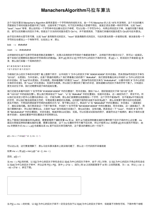
接下来我们还需要和处理后的字符串t等长的数组p,其中 p[i] 表⽰以 t[i] 字符为中⼼的回⽂⼦串的半径,若 p[i] = 1,则该回⽂⼦串就是 t[i] 本⾝,那么我们来看⼀个简单的例⼦:# 1 # 2 # 2 # 1 # 2 # 2 #1 2 1 2 5 2 1 6 1 2 3 2 1为啥我们关⼼回⽂⼦串的半径呢?看上⾯那个例⼦,以中间的 '1' 为中⼼的回⽂⼦串 "#2#2#1#2#2#" 的半径是6,⽽未添加#号的回⽂⼦串为"22122",长度是5,为半径减1。
An Algorithm for Mixed Integer Optimization #
2
M. Koppe ¨ and R. Weismantel
setting, but also that there is no finite cutting plane algorithm known for general mixed integer programs, except for the special case when the support of the linear objective function vector is contained in the subset of the integer variables. We refer to Gomory [4], Balas, Ceria, and Cornu´ ejols [2], and Nemhauser and Wolsey [9] for cutting plane algorithms applicable to mixed integer programs involving 0/1 or general integer variables. We propose in this paper a purely primal approach that extends the earlier work of Haus, Koppe, ¨ and Weismantel [6, 7] from the pure integer setting to a mixed integer linear optimization problem. More precisely, we assume that a primal feasible solution is at hand. This is then turned into a basic feasible solution of an appropriate tableau. Iteratively we reformulate the tableau by eliminating columns with negative reduced cost and adding new columns in a way that a representation of the original feasible set is maintained. This extension from integer to mixed integer programs requires a couple of geometric arguments that one can neglect in the pure integer setting. We begin in Section 2 with our tableau setting. In particular, we introduce the standard form of a tableau that we associate with a primal feasible solution. Section 3 introduces a general scheme of “reformulating” mixed-integer programs by using “mixed-integral generating sets.” This notion will be explained in Definition 3.2. By a reformulation step we mean the operation of replacing a set of columns of negative reduced cost by a set of new columns in a way that every feasible solution that involves the variables associated with the columns to be removed can be expressed as a non-negative mixed-integer combination of the new columns. Section 4 deals with a specific algorithm that works along the rows of the tableau. For a particular row of our system we perform a reformulation step. Unfortunately this procedure might not terminate in finite time, because of the phenomenon of zigzagging as we show on an example. This example also motivates our refined approach that we outline in Sections 5 and 6. Here we work simultaneously with several rows of the given tableau. This however requires a price to pay that the column replacement operation becomes significantly more involved. The award of using the more involved replacement step is that the resulting algorithm becomes finite which is the maximum we can expect for mixed integer programs if we believe in complexity theory.
马拉车算法——精选推荐

马拉车算法Manacher Algorithm算法,俗称马拉车算法,其时间复杂为O(n)。
该算法是利⽤回⽂串的特性来避免重复计算的。
在时间复杂度为O(n^2)的算法中,我们在遍历的过程要考虑到回⽂串长度的奇偶性,⽐如说“abba”的长度为偶数,“abcba”的长度为奇数,这样在寻找最长回⽂⼦串的过程要分别考奇偶的情况,是否可以统⼀处理了?⼀)第⼀步是改造字符串S,变为T,其改造的⽅法如下:在字符串S的字符之间和S的⾸尾都插⼊⼀个“#”,如:S=“abba”变为T="#a#b#b#a#" 。
我们会发现S的长度是4,⽽T的长度为9,长度变为奇数了!!S的长度为奇数时,S=“abcba”,变化为T=“#a#b#c#b#a#”,T的长度为11,所以我们发现其改造可以将字符串的长度变为奇数,这样就可以统⼀的处理奇偶的情况了。
⼆)第⼆步,为了改进回⽂相互重叠的情况,我们将改造完后的T[ i ] 处的回⽂半径存储到数组P[ i ]中(P[ i ]表⽰以字符T[ i ]为中⼼的最长回⽂字串的最端右字符到T[ i ]的长度),这样最后遍历数组P,取其中最⼤值即可。
举⼀个简单的例⼦感受⼀下:数组P有⼀性质,P[ i ] - 1就是该回⽂⼦串在原字符串S中的长度,⾄于证明,⾸先在转换得到的字符串T中,所有的回⽂字串的长度都为奇数,那么对于以T[ i ]为中⼼的最长回⽂字串,其长度就为2*P[ i ]-1, 经过观察可知,T中所有的回⽂⼦串,其中分隔符的数量⼀定⽐其他字符的数量多1,也就是有P[ i ]个分隔符,剩下P[ i ]-1个字符来⾃原字符串,所以该回⽂串在原字符串中的长度就为P[ i ]-1。
另外,由于第⼀个和最后⼀个字符都是#号,且也需要搜索回⽂,为了防⽌越界,我们还需要在⾸尾再加上⾮#号字符,实际操作时我们只需给开头加上个⾮#号字符,结尾不⽤加的原因是字符串的结尾标识为'\0',等于默认加过了。
稀疏恢复和傅里叶采样
Accepted by . . . . . . . . . . . . . . . . . . . . . . . . . . . . . . . . . . . . . . . . . . . . . . . . . . . . . . . . . . . . . . . . . . . . . . . . . . . . . . Leslie A. Kolodziejski Chair, Department Committee on Graduate Students
2
Sparse Recovery and Fourier Sampling by Eric Price
Submitted to the Department of Electrical Engineering and Computer Science on August 26, 2013, in partial fulfillment of the requirements for the degree of Doctor of Philosophy in Computer Science
Author . . . . . . . . . . . . . . . . . . . . . . . . . . . . . . . . . . . . . . . . . . . . . . . . . . . . . . . . . . . . . . . . . . . . . . . . . . . . . . . . . . . Department of Electrical Engineering and Computer Science August 26, 2013
Certified by . . . . . . . . . . . . . . . . . . . . . . . . . . . . . . . . . . . . . . . . . . . . . . . . . . . . . . . . . . . . . . . . . . . . . . . . . . . . . . . Piotr Indyk Professor Thesis Supervisor
热值仪中文说明

List of Illustrations------------------------------------------------------------- v
Chapter 1-------------------------------------------------------------------------- 1
符号
文件符号定义
标签
说明
WARNING
包括条件、惯例和步骤必须谨慎执行, 以防人员伤害和设备损坏。
CAUTION
包括条件、惯例和步骤必须谨慎执行, 以防人员伤害和设备损坏
CAUTION
电击或高温部分危险,如不采取适当的 警告,可导致人员伤害。
CAUTION
静电感应元件,要求正确地触摸,以防 损坏。
Flo-Cal 用户手册
ii 索引
Chapter 4 --------------------------------------------------------------------------17
Installation ....................................................................................................... 17 System Mounting .............................................................................................. 17 Unpacking and Inspection .................................................................... 17 Wall Mount Preparation and Procedure ............................................... 18 Free Standing Mount Instructions ........................................................ 20 Electrical Installation......................................................................................... 21 Gas & Air Supply Installation ........................................................................... 22
UVM1.1应用指南及源代码分析_20111211版
6.2. 强大的config .............................................................................................94
6.3. 聚合config变量 .........................................................................................98
写这本书,只是想把自己会的一点东西完全的落于纸上。在努力学习 UVM 的 过程中,自己花费了很多时间和精力。我只想把学习的心得记录下来,希望能够给 后来的人以启发。如果这本书能够给一个人带来一点点的帮助,那么我的努力就不 算是白费。
这本书的前半部分(第 1 到第 9 章)介绍了 UVM 的使用,其用户群较为广泛;
8.2. 搭建一个简单的register model...............................................................129
8.3. 复杂的register model...............................................................................137
函数索引609xvi图目录图11uvm在数字电路设计中的位置3图12uvm对systemverilog的封装4图13简单验证平台5图14uvm验证平台的树形结构6图15实际验证平台7图16packbytes和unpackbytes14图17uvm验证平台中的agent181图21完整的uvm树35图22uvm中常用类的继承关系37图31uvm中的常用phase47图32uvm中所有的phase50图33两个driver位于同一domain57图34两个driver位于不同的domain58图41穿梭的transaction60图51defaultsequence的设置与启动77图52sequencer与driver之间的通信80图53virtualsequence的使用85图61半全局变量93图71monitor与scoreboard的通信104图72使用public成员变量实现通信105图73put操作106图74get操作106xvii图75transport操作107图76component在端口通信中的作用109图77connect关系的建立110图78port与imp的连接111图79portexport与imp的连接115图710使用fifo连接component122图81uvmregfield和uvmreg126图82使用registermodel读取寄存器的流程128图83uvmregfield
- 1、下载文档前请自行甄别文档内容的完整性,平台不提供额外的编辑、内容补充、找答案等附加服务。
- 2、"仅部分预览"的文档,不可在线预览部分如存在完整性等问题,可反馈申请退款(可完整预览的文档不适用该条件!)。
- 3、如文档侵犯您的权益,请联系客服反馈,我们会尽快为您处理(人工客服工作时间:9:00-18:30)。
4096IEEE TRANSACTIONS ON MAGNETICS, VOL. 43, NO. 12, DECEMBER 2007A Linear Algorithm for Tracing Magnet Position and Orientation by Using Three-Axis Magnetic SensorsChao Hu1;3 , Max Q.-H. Meng2;3 , and Mrinal Mandal1Department of Electrical and Computer Engineering, University of Alberta, Edmonton, AB T6G 2V4, Canada Department of Electronic Engineering, The Chinese University of Hong Kong, Shatin, Hong Kong Institute of Advanced Integration Technology/Shenzhen Institute of Advanced Technology, Shenzhen 518067, ChinaFor medical diagnoses and treatments, it is often desirable to wirelessly trace an object that moves inside the human body. A magnetic tracing technique suggested for such applications uses a small magnet as the excitation source, which does not require the power supply and connection wire. It provides good tracing accuracy and can be easily implemented. As the magnet moves, it establishes around the human body a static magnetic field, whose intensity is related to the magnet’s 3-D position and 2-D orientation parameters. With magnetic sensors, these magnetic intensities can be detected in some predetermined spatial points, and the position and orientation parameters can be computed. Typically, a nonlinear optimization algorithm is applied to such a problem, but a linear algorithm is preferable for faster, more reliable computation, and lower complexity. In this paper, we propose a linear algorithm to determine the 5-D magnet’s position and orientation parameters. With the data from five (or more) three-axis magnetic sensors, this algorithm results in a solution by the matrix and algebra computations. We applied this linear algorithm on the real localization system, and the results of simulations and real experiments show that satisfactory tracing accuracy can be achieved by using a sensor array with enough three-axis magnetic sensors. Index Terms—Linear algorithm, magnet’s position and orientation, magnetic tracing.I. INTRODUCTIONRECENTLY, many researchers have suggested the magnetic tracing (MT) technique in medical applications [1]–[8]. This is because the human body has a magnetic permeability very close to that of air, water, or nonferromagnetic material, and exerts very little influence on the static (or low-frequency) magnetic field, such that it is possible to achieve high tracing accuracy. Nevertheless, the MT technique is of higher speed and easier realization compared to other possible techniques, e.g., computer tomography, magnetic resonance imaging, and 3-D ultrasonic techniques. Typically, this technique uses magnetic excitation sources, which can be created by one single magnetic dipole (or coil), or two or three orthogonal magnetic dipoles (or coils). The magnetic field signals produced by these dipoles can be measured by the magnetic sensors (or receiving coils) arranged in some positions around the human body. With the measured sensor data, the tracing parameters can be computed using an appropriate algorithm. In some specific applications, it is difficult to use cabled equipment, making the wireless technique preferable, e.g., the tracking of wireless capsule endoscopes [9], and the monitoring of the pill transit [10]–[15]. Since such applications demand as low a power and space as possible, a permanent magnet is therefore a reasonable choice to serve as the excitation dipole [9], [11], [13]–[15] instead of the electric current coil [16]–[21]. The magnetic field created by a permanent magnet is a highorder nonlinear function of the 5-D magnet’s position and orientation parameters. To solve such a problem, the nonlinear least square optimization algorithm is a common method [10]–[15].However, the nonlinear optimization method has its limitations. First, it must have an initial estimation of the parameters (or their bounds), to begin the search for the optimum. If the initial parameters have a large error, the algorithms might fail to give a correct global solution because the mathematic model of the magnetic dipole has many local minima. Second, the searching process takes a long time, meaning that there is not enough time to apply other signal processing measures to improve the tracing accuracy. Third, the computation complexity might be so high that it becomes difficult to be realized in a real-time instrument. All these problems can be solved by a linear algorithm. Therefore, in this paper, we propose a linear algorithm for the magnet’s localization and orientation using five or more three-axis magnetic sensors. The proposed algorithm is derived by the absolute vector computation, so no calculation error is induced by the approximations in the equation derivation. The organization of this paper is as follows. In Section II, we introduce the mathematical model of the magnetic field produced by a permanent magnet. In Section III, we propose the linear algorithm. In Section IV, we present the performance of the algorithm by an example and the results of simulation and real experimentation, which is followed by the conclusions in Section V. II. NONLINEAR MATHEMATIC MODEL Fig. 1 shows a cylindrical magnet with length , diameter , and a uniform magnetization (Amp/meter) on the top and bottom surfaces. Let be the vector that represents a spatial point with respect to the magnet center position . The magnetic flux density at this point can be calculated as [22] (1)Digital Object Identifier 10.1109/TMAG.2007.907581 Color versions of one or more of the figures in this paper are available online at .where ability of the medium,is the relative permeis the magnetic permeability0018-9464/$25.00 © 2007 IEEEHU et al.: A LINEAR ALGORITHM FOR TRACING MAGNET POSITION AND ORIENTATION4097is orthogonal to , making the dot product Because , we get on both sides of the above equation with (8) That isFig. 1. Coordinate system for magnet’s localization: (a; b; c) is the position of is the direction of the magnet. p = (x ; y ; z ) represents a the magnet, spatial point.H(9) of the air, and is the normalized vector representing the orientation of the magnet’s magnetism. Assume that there are magnetic sensors, with th sensor located at . The magnetic flux density at the th sensor location can be represented by (2) , and are the magnetic components in the where three orthogonal coordinate axes, and could be represented by We observe that in this equation, the magnitudes of these vecand are irrespective to the solution. However, tors it gives some relative relations of the parameters of these vectors. This means that we cannot get the unique true solution only using (8). To get the unique solution, we need to use other constraints (these constraints are defined by (6), (28), (29), and will be further presented below). Expanding (9), we have(10) (3) It can be further simplified as (11) where (5) (12) . where Note that there are six unknown parameters . The flux intensity is invariant to the rotation of the magnet along its major axis. Hence, the magnet’s orientation is in two dimensions, in other words, the length of vector can be any fixed value. Therefore, we add the following constraint to : (6) , and Since the magnetic intensity components can be measured by the magnetic sensors, we can apply a nonlinear algorithm to solve for the six localization and orientation parameters using these equations. The most common approach is to define an objective error function by changing (3)–(6) into the form of summation of square errors, and applying an optimization algorithm to find the parameters that minimize the error function (the least square error method) [9]. However, as mentioned in Section I, the nonlinear algorithm has its limitations, so instead we propose a linear algorithm. III. LINEAR ALGORITHM A. Derivation of the Linear Model Because sides of (1) with , making the cross product on both , we have (7) (13) (14) . In (11), and are funcwith in the tions of the magnetic components , and independent of the six unspatial position is only composed of known parameters the six unknown parameters. In some predetermined posi, we can dispose three-axis tions magnetic sensors to measure the magnetic components , and , such that and can be determined. Therefore, with five three-axis magnetic sensors, a matrix and a vector are formed, and then we solve for (15) We have tested the solution with the simulations using different conditions, and found that the unique solution can be obis nonsingular. In cases in which is tained if the matrix singular, we take the following measures. , and , then we 1) We define , and : have different representations of (16) (17) (18)(4)4098IEEE TRANSACTIONS ON MAGNETICS, VOL. 43, NO. 12, DECEMBER 2007or we define then, and, and (19) (20) (21)The matrix is singular (we can verify ), but its rank is two, so we can get two independent equations (26) (27) To solve for parameter , we need to find another equation. Dividing (3) and (4) with (5), we have the following two equations:2) Weusesix,ormorethansix,three-axismagneticsensors.Becausethesensornumberismorethanthenumberofunknown parameters,thesingularitycanbeavoidedifthesesensorsare arranged in specifically-selected spatial positions. Once is solved, the magnet’s position and orientation parameters , and can further be solved. This method is much simpler than solving nonlinear equations (3)–(6) directly. The solution is also irrelevant to the magnetization of the magnet and the relative permeability of the medium. The cost of this method is that it requires five three-axis sensors as a minimum, while the nonlinear method could use five sensors that could be one-axis, or two-axis or three-axis sensors. B. Algorithm for Magnetic Sensor Array Although five three-axis magnetic sensors are enough for solving (11), more sensors are preferable to get higher tracking accuracy, because the accuracy is influenced by the interferences in the sensor signals, especially in the case of low signal-to-noise ratio (SNR). From (1), we observe that magnetic intensity is an inverse function with the power of three of the distance from the magnet to the sensor. In order to obtain stronger sensor signals for high SNR, we should control this distance with more densely distributed sensors. To simplify the problem, these sensors can be arranged in a plane so as to form a sensor array [9], [13], [16]. When there are more than five sensors, we can apply the following optimal fitting method. Assume there are totally three-axis sensors, we change the expression of (11), and define the fitting error to be . The optimal solution of which makes minimum is (22) is 5 where element is with and th element is given by (14). 5 matrix, in which the th row and th column given by (12); is a vector, in which the with(28) and(29) Let (26) and (27) be substituted into (28) and (29), giving us the following 2-order equations with one unknown : (30) (31) are the functions of known as well as the solutions of . We can select any one, or two equations to solve , among the 2 equations defined by (30) or (31). Here, we present a more accurate method to determine by applying the least square error method. We define an error to be (32) Using this equation, three roots of can be solved for a minimum of . If there are two imaginary roots and one real root (in most cases), the solution is the real root; if all three roots are real, they are tried in (32), and the solution is chosen as the one with the minimum of . With this , we can compute and by (26) and (27). D. Determine the Sign of the Orientation From (23), we know that the calculated orientation parameter (and ) could be positive or negative. This is not true in real cases, where the magnet has its unique magnetic direction from one surface to another surface. Hence, we need to determine the sign of the orientation. Here, we first show that the sign of the does not affect the calculation of orientation . the location parameters and , (28) and (29) can be Using rewritten as where data andC. Solution of the Magnet Position and Orientation Now we have the solutions of (6), we get the orientation . From (23) (24) (25) Here, the orientation might have a positive or negative sign. We will discuss how to determine this sign in Step D below. , from (10), we have For the magnet position(33)(34)HU et al.: A LINEAR ALGORITHM FOR TRACING MAGNET POSITION AND ORIENTATION4099Because are calculated using these two equations and , the sign of does not the solution of . affect the calculation results of and Now, with the calculated results of , we define and calculateUsing the sensor positions and the above sensor outputs, , which is singular because we get the matrix and and are infinite. Here, we adopt (16)–(18), and the solutions of is . Then the orientation is calculated as(35)(36)(37) From (3)–(5), we know (38) (39) (40) Then, it is clear thatwhere the sign of orientation is wrong as compared to given data, so we will adjust it later. With this orientation, we calculate the parameter by the least square error method [in (32)], , and and reach three roots: . The solution is the real root, we obtain the parameter . Then, two other position parameters can be solved as , and . With these parameters, we findsuch thatis negative. That is(41) Therefore, the sign of the orientation can be determined. If ; else . When the sign of is determined, the signs and can also be adjusted. Therefore, the six unknowns are solved. IV. PERFORMANCE EVALUATION BY SIMULATION AND EXPERIMENTS In this section, we evaluate the performance of the proposed algorithm by giving an example and the results of simulation and real experiments. A. Example Here, an example is presented for five three-axis sensors to be applied to the localization and orientation. The five sensors are located in and (in meters). The magnet’s position and orientation is given as . From (3)–(5), we get 5-sensor outputs (relative to ) asHence, the resultant localization and orientation parameters are . This is exactly the same as the pre-setup parameters. B. Simulation for Denoising Ability The algorithm was tested in MATLAB programs, which uses magnetic intensities created by some magnets’ positions and directions. To test the anti-interference ability of the algorithm, white-noise was added in the simulated sensor signals. The algorithm is tested using 5, 9, and 16 sensors. For the 5-sensors’ case, the sensors are arranged on the center and 0.2 m. In four corners of a square plane with an area of 0.2 m the case of 9-sensors and 16-sensors, the sensors are uniformly arranged on the square plane of 0.2 m 0.2 m and 0.24 m 0.24 m, as shown in Figs. 2 and 3. To evaluate the performances, we define the localization error and orientation error to be (42) (43) Figs. 4–6 show simulation results of the localization error via the noise level in the magnetic intensity. Here, we represent the noise relative to the magnet’s constant . In the 5-sensor case, the localization (position) errors are too large ( mm) if the noise level is larger than 18. This error is much improved when more sensors are used. As shown in Figs. 5 and 6, when the noise level is within 65 times of Bt, the localization error is smaller than 18 mm in the 9-sensors case, and 3 mm in the 16-sensors case.of4100IEEE TRANSACTIONS ON MAGNETICS, VOL. 43, NO. 12, DECEMBER 2007Fig. 2. Arrangement of 9-sensors.Fig. 6. Localization accuracy by 16-sensors.Fig. 3. Arrangement of 16-sensors. Fig. 7. 3-D localization results.Fig. 4. Localization accuracy by 5-sensors.Fig. 8. 2-D (X-Y plane) localization results.Fig. 5. Localization accuracy by 9-sensors.C. Real Experiment We built an experimental system, which includes magnetic (Hall) sensors, a precision amplification circuit, a stabilized power source, AD converters, and a PC computer. The sixteen three-axis sensors are fixed in a plane such that a 2-D array is formed as illustrated in Fig. 3. We get sensing data from these sensors when the magnet is located in some spatial positions and orientations that can be determined. These data are filteredusing moving average techniques so that they produce much less noise. Figs. 7 and 8 show the 3-D and 2-D localization results. Figs. 9 and 10 show the localization and orientation errors at different positions. We observe that within the sensor area, the localization error is within 8 mm, and the orientation error is within 7%. The average localization error is 5.6 mm and the average orientation error is 2.9% (around 1.7 ). While comparing to the nonlinear algorithm, similar accuracy (5.6 mm, 4.26% in nonlinear algorithm [9]) is obtained for cases in which the nonlinear algorithm adopts a proper initial guess of the parameters. However, the execution speed of the proposed linear algorithm is much faster. Through the simulation, we observed that the execution time is only one tenth of that of the fastest nonlinear algorithm, so that the linear algorithm can provide greater capacity for signal processing to obtain further improved accuracy.HU et al.: A LINEAR ALGORITHM FOR TRACING MAGNET POSITION AND ORIENTATION4101Fig. 9. Localization error.Fig. 10. Orientation error.V. CONCLUSION A linear algorithm is proposed to calculate a magnet’s position and orientation. This algorithm is realized by simple matrix and algebraic calculations, and can be applied to the magnetic sensor array composed of five or more three-axis magnetic sensors. Higher accuracy can be obtained with denser sensor arrangements. In addition, a real test system has been built by an array of sixteen three-axis Hall sensors, and results are satisfactory. Compared to the nonlinear algorithms, this algorithm has faster speed, lower complexity, and higher reliability. Using this algorithm, we are now building a real time system for tracking a capsule that moves in the human GI tract. ACKNOWLEDGMENT This project was supported by RGC Competitive Earmarked Research Grant #CUHK4213/04E of the Hong Kong government, awarded to Max Meng. REFERENCES[1] NDI Aurora Electromagnetic Tracking System. [Online]. Available: /aurora.php [2] Ascension Technol. Corp. Products Application. [Online]. Available: /products/microbird.php [3] D. D. Frantz, A. D. Wiles, S. E. Leis, and S. R. Kirsch, “Accuracy assessment protocols for electromagnetic tracking systems,” Phys. Med. Biol., vol. 48, pp. 2241–2251, 2003.[4] K. Schicho, M. Figl, M. Donat, W. Birkfellner, R. Seemann, A. Wagner, H. Bergmann, and R. Ewers, “Stability of miniature electromagnetic tracking systems,” Phys. Med. Biol., vol. 50, pp. 2089–2098, 2005. [5] J. Hummel, M. Figl, C. Kollmann, and H. Bergmann, “Evaluation of a miniature electro-magnetic position tracker,” Med. Phys., vol. 29, no. 10, pp. 2205–2212, 2002. [6] K. H. Wong, J. Tang, S. Dieterich, H. Zhang, T. Zhou, and K. Cleary, “Respiratory motion compensation studies using a 3D robotic motion simulator and optical/electromagnetic tracking technologies,” in 2004 IEEE Nucl. Sci. Symp. Conf., Rome, Italy, Oct. 22–26, 2004. [7] D. C. Barratt, A. H. Davies, A. D. Hughes, S. A. Thom, and K. N. Humphies, “Optimisation and evaluation of an electromagnetic tracking device for high-accuracy three-dimensional ultrasound imaging of the carotid arteries,” Ultrasound Med. Biol., vol. 27, no. 7, pp. 957–968, Jul. 2001. [8] Y. Yamada, N. Yoshida, K. Kobayashi, and K. Yamauchi, “An application of magnet and magnetic sensor: Measurement system for tooth movement,” IEEE Trans. Biomed. Eng., vol. 37, no. 10, pp. 919–924, Oct. 1990. [9] C. Hu, M. Q.- H. Meng, and M. Mandal, “Efficient magnetic localization and orientation technique for capsule endoscopy,” Int. J. Inf. Acquisition, vol. 2, no. 1, pp. 23–36, 2005. [10] W. Weitschies, M. Karaus, D. Cordini, L. Trahms, J. Breitkreutz, and W. Semmler, “Magnetic marker monitoring of disintegrating capsules,” Eur. J. Pharm. Sci., vol. 13, no. 4, pp. 411–416, Jul. 2001. [11] W. Weitschiles, R. Kotitz, DinoCordini, and L. Trahms, “High-resolution monitoring of the gastro-intestinal transit of a magnetic marked capsule,” J. Pharm. Sci., vol. 86, no. 1, pp. 1218–1222, 1997. [12] W. Weitschies, J. Wedmeyer, R. Stehr, and L. Trahms, “Magnetic markers as a noninvasive tool to monitor gastrointestinal transit,” IEEE Trans. Biomed. Eng., vol. 41, no. 2, pp. 192–195, Feb. 1994. [13] V. Schlageter, P.-A. Besse, R. S. Popovic, and P. Kucera, “Tracking system with five degrees of freedom using 2D-array of Hall sensors and a permanent magnet,” Sens. Actuators, vol. 92, pp. 37–42, 2001. [14] N. Mani Prakash and F. A. Spelman, “Localization of a magnetic marker for GI motility studies: An in vitro feasibility study,” in Proc. 19th Annu. Int. Conf. IEEE Eng. Medicine Biol. Soc., Chicago, IL, Oct. 30–Nov. 2, 1997, pp. 2394–3239. [15] W. Andra, H. Danan, W. Kirmße, H.-H. Kramer, P. Saupe, R. Schmieg, and M. E. Bellemann, “A novel method for real-time magnetic marker monitoring in the gastrointestinal tract,” Phys. Med. Biol., vol. 45, pp. 3081–3093, 2000. [16] A. Plotkin and E. Paperno, “3D magnetic tracking of a single subminiature coil with a large 2-D array of uniaxial transmitters,” IEEE Trans. Magn., vol. 39, no. 5, pp. 3295–3297, Sep. 2003. [17] J. E. McFee and Y. Das, “Determination of the parameters of a dipole by measurement of its magnetic field,” IEEE Trans. Antennas Propag., vol. AP-29, no. 2, pp. 282–287, Mar. 1981. [18] Y. Liu, Y. Wang, D. Zhou, X. Hu, and J. Wu, “Study on an experimental AC electromagnetic tracking system,” in Proc. 5th World Congr. Intelligent Control Autom., Hangzhou, China, Jun. 15–19, 2004. [19] F. H. Raab, E. B. Blood, T. O. Steiner, and H. R. Jones, “Magnetic position and orientation tracking system,” IEEE Trans. Aerosp. Electron. Syst., vol. AES-15, no. 5, pp. 709–718, Sep. 1979. [20] E. Paperno, I. Sasada, and E. Leonovich, “A new method for magnetic position and orientation tracking,” IEEE Trans. Magn., vol. 37, no. 4, pp. 1938–1940, Jul. 2001. [21] H. P. Kalmus, “A new guiding and tracking system,” IRE Trans. Aerosp. Navig. Electron., vol. 9, pp. 7–10, Mar. 1962. [22] D. K. Cheng, Field and Wave Electromagnetics: Static Magnetic Fields. Reading, MA: Addison-Wesley, 1989.Manuscript received November 23, 2005; revised August 28, 2007. Corresponding author: C. Hu (e-mail: hcsfds@ece.ualberta.ca; hu.chao.hu@gmail. com).。
