[1998 ] FACTORING WAVELET TRANSFORMS INTO LIFTING STEPS
3500系列_中文手册
1.13.3 程序概要页 .................................................................................................... 29
1.13.4 报警概要......................................................................................................... 31
2.
2.1.1 2.1.2 2.1.3 2.2
第 2 章 访问更多的参数 .................................................33
等级 3(Level 3)......................................................................................... 33 配置等级......................................................................................................... 33 选择不同的访问等级................................................................................... 34 访问菜单中的参数 .........................................................................................35
1.1 这是什么样的仪表? .........................................................................................9
脊波理论_从脊波变换到Curvelet变换

762
工程数学学报
第22卷
2 脊波理论产生的背景
我们先从函数逼近论的角度来剖析脊波理论产生的背景。 对于 Sobolev 函数类,有如下定理[4]: 定理2.1 记定义于环 T 上的函数类 F = {f, f Hs(T ) ≤ 1},设 f ∈ F ,对于任一正交 基 (φi)i∈I ,令 QM (f ) 表示此正交基对函数 f 的 M 项非线性逼近,即,
第5期
焦李成等:脊波理论: 从脊波变换到 Curvelet 变换
763
下界。而三角基则不然。小波分析比傅立叶分析能更“稀疏”地表示一维分段光滑或者有界变 差函数。这就是小波分析在众多学科领域中取得巨大成功的一个关键原因。
遗憾的是,小波分析在一维时所具有的优异特性并不能简单的推广到二维或更高维。考虑 一个简单二维图像模型[6]:
本文主要综述脊波理论的产生、发展历程,并阐述目前亟待解决的问题。
收稿日期: 2005-06-04. 作者简介: 焦李成(1959年生),男,教授,博士生导师,IEEE高级会员,研究方向:智 能信息处理.
∗基金项目: 国家自然科学基金(No.60073053);国家“863”计划(No.2002AA135080):“十五”国防预研项目 (No.413070504).
Gamma
上的测度。
定理3.3 (Parseval 关系) 设 f ∈ L1 ∪ L2(Rn) 且 ψ 满足容许条件,则:
f
2 2
=
cψ
·
2
< f, ψγ > µ(dγ).
(15)
因为 L1 ∪ L2(Rn) 在 L2(Rn) 中稠,于是有: 命题3.1 对于 ∀f, g ∈ L2(Rn),
< f, g >= cψ R(f )R(g)(γ)µ(dγ).
小波变换与尺度函数

小波分析里,很容易混淆的一个概念就是小波函数(wavelet function)和尺度函数(scaling function)的关系。
本文将不涉及小波分析的由来及发展历史,也不谈小波分析应用,本文主要目标仅是试着解释清楚小波函数和尺度函数两者的关系,同时也解释一些小波分析中的其他必要相关概念。
当然,要更好理解小波分析,一些傅里叶变换的知识是必要的。
我们知道,傅里叶变换分三种不同但又紧密相连的形式:1,积分傅里叶变换,时域频域都连续;2,傅里叶级数展开,时域连续,频域离散;3,离散傅里叶变换,时域频域都离散。
同样,在小波分析中,也有三种类似的形式。
积分(连续)小波变换(CWT),小波级数展开,以及离散小波变换(DWT)。
先看看连续小波变换,连续小波正变换为[1]:(1)逆变换为:(2)其中*号表示复共轭,为小波基函数(basis function)。
不同小波基函数,都是由同一个基本小波(basic wavelet)ψ(t),经缩放和平移生成,即:(3)傅里叶变换把一个信号f(t)分解为一系列不同频率正弦型信号的叠加,而傅里叶变换系数就代表不同正弦型信号的幅值。
其中,所有正弦型基函数都由傅里叶基函数生成。
类似于傅里叶基函数,所有小波基函数也由同一个基本小波生成[2]。
不同的是,傅里叶基函数是固定的正弦型信号,而基本小波并未指定,需要根据实际的信号形式,在满足基本小波约束条件下进行设计。
可以看到,连续小波变换采用积分形式,而实际应用中,我们计算的都是采样后的信号,也需要通过离散形式来处理和表达,所以更加有用的是时域频域都离散的DWT,离散小波变换。
但是离散小波变换的计算将引入三个问题:1,数据冗余。
观察式(1),可以看到,小波变换将一个一维信号变换为二维小波系数。
同样,若信号是二维,变换后将得到三维小波系数。
这反映了小波变换的优点,变换不仅具有傅里叶变换的频域分辨率,同时具有了时域或空域分辨率。
但是一维信号用二维系数来表达,这就意味着必然有很大的冗余性。
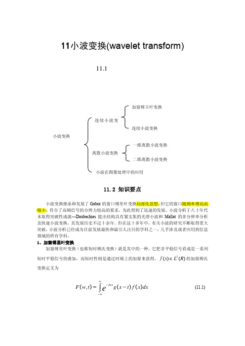
小波变换(wavelet transform)
其中,左上角的元素表示整个图像块的像素值的平均值,其余是该图像块的细节系数。 如果从矩阵中去掉表示图像的某些细节系数,事实证明重构的图像质量仍然可以接受。 具体做法是设置一个阈值,例如的细节系数δ≤5 就把它当作“0”看待,这样相比, Aδ 中“0”的数目增加了 18 个,也就是去掉了 18 个细节系数。这样做的好 处是可提高小波图像编码的效率。对矩阵进行逆变换,得到了重构的近似矩阵
7 50 42 31 39 18 10 63
57 16 24 33 25 48 56 1
使用灰度表示的图像如图 11.2 所示:
图 11.2 图像矩阵 A 的灰度图
一个图像块是一个二维的数据阵列, 可以先对阵列的每一行进行一维小波变换, 然后对 再行变换之后的阵列的每一列进行一维小波变换, 最后对经过变换之后的图像数据阵列进行 编码。 (1) 求均值与差值 利用一维的非规范化哈尔小波变换对图像矩阵的每一行进行变换, 即求均值与差值。 在 图像块矩阵 A 中,第一行的像素值为 R0: [64 2 3 61 60 6 7 57] 步骤 1:在 R0 行上取每一对像素的平均值,并将结果放到新一行 N0 的前 4 个位置, 其余的 4 个数是 R0 行每一对像素的差值的一半(细节系数) : R0: [64 2 3 61 60 6 7 57] N0: [33 32 33 32 31 -29 27 -25] 步骤 2:对行 N0 的前 4 个数使用与第一步相同的方法,得到两个平均值和两个细节系 数,并放在新一行 N1 的前 4 个位置,其余的 4 个细节系数直接从行 N0 复制到 N1 的相应 位置上: N1: [32.5 32.5 0.5 0.5 31 -29 27 -25] 步骤 3:用与步骤 1 和 2 相同的方法,对剩余的一对平均值求平均值和差值, N2: [32.5 0 0.5 0.5 31 -29 27 -25] 3 0 0 1 V : V W W W2 其中,第一个元素是该行像素值的平均值,其余的是这行的细节系数。 (2) 计算图像矩阵 使用(1)中求均值和差值的方法,对矩阵的每一行进行计算,得到行变换后的矩阵:
图像处理和计算机视觉中的经典论文
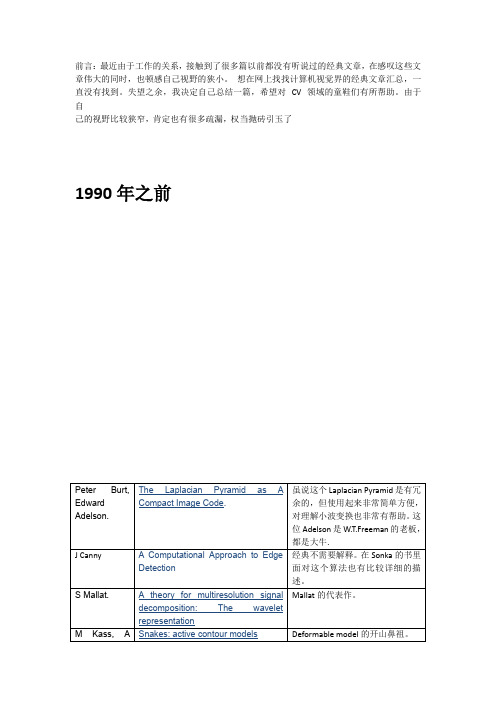
前言:最近由于工作的关系,接触到了很多篇以前都没有听说过的经典文章,在感叹这些文章伟大的同时,也顿感自己视野的狭小。
想在网上找找计算机视觉界的经典文章汇总,一直没有找到。
失望之余,我决定自己总结一篇,希望对 CV领域的童鞋们有所帮助。
由于自
己的视野比较狭窄,肯定也有很多疏漏,权当抛砖引玉了
1990年之前
1990年
1991年
1992年
1993年
1994年
1995年
1996年
1997年
1998年
1998年是图像处理和计算机视觉经典文章井喷的一年。
大概从这一年开始,开始有了新的趋势。
由于竞争的加剧,一些好的算法都先发在会议上了,先占个坑,等过一两年之后再扩展到会议上。
1999年
2000年
世纪之交,各种综述都出来了
2001年
2002年
2003年
2004年
2005年
2006年
2007年
2008年
2009年
2010年
2011年
2012年。
The Wavelet Transform in Multivariate Data Analysis

Using the Wavelet T ransform for Multivariate Data Analysis andTime Series ForecastingFionn Murtagh(1)and Alex Aussem(2)(1)University of Ulster,Faculty of Informatics,Londonderry BT487JL,Northern Ireland. Email fd.murtagh@(2)Universit´e Ren´e Descartes,UFR de Math´e matiques et Informatique,45,rue des Saints-P`e res,75006Paris,France.Email alex@math-info.univ-paris5.frAbstract:We discuss the use of orthogonal wavelet transforms in multivariate data anal-ysis methods such as clustering and dimensionality reduction.Wavelet transforms allow us to introduce multiresolution approximation,and multiscale nonparametric regres-sion or smoothing,in a natural and integrated way into the data analysis.Applications illustrate the powerfulness of this new perspective on data analysis.Keywords:Wavelet Transform,Additive Decomposition,Partitioning,Clustering,Di-mensionality Reduction,Data Display,Exploratory Data Analysis,Principal Components Analysis,Preliminary Data Transformation1IntroductionData analysis,for exploratory purposes,or prediction,is usually preceded by various data transformations and recoding.In fact,we would hazard a guess that90%of the work involved in analyzing data lies in this initial stage of data preprocessing.This includes:problem demarcation and data capture;selecting non-missing data of fairly homogeneous quality;data coding;and a range of preliminary data transformations.The wavelet transform offers a particularly appealing data transformation,as a pre-liminary to data analysis.It offers additionally the possibility of close integration into the analysis procedure as will be seen in this article.The wavelet transform may be used to “open up”the data to de-noising,smoothing,etc.,in a natural and integrated way.2Some Perspectives on the Wavelet TransformWe can think of our input data as a time-varying signal,e.g.a time series.If discretely sampled(as will almost always be the case in practice),this amounts to considering an input vector of values.The input data may be sampled at discrete wavelength values, yielding a spectrum,or one-dimensional image.A two-dimensional,or more complicated input image,can be fed to the analysis engine as a rasterized data stream.Analysis of such a two-dimensional image may be carried out independently on each dimension,but such an implementation issue will not be of further concern to us here.Even though our1motivation arises from the analysis of ordered input data vectors,we will see below that we have no difficulty in using exactly the same approach with(more common)unordered input data vectors.Wavelets can be introduced in different ways.One point of view on the wavelet trans-form is by means offilter banks.Thefiltering of the input signal is some transformation of it,e.g.a low-passfilter,or convolution with a smoothing function.Low-pass and high-passfilters are both considered in the wavelet transform,and their complementary use provides signal analysis and synthesis.3The Wavelet Transform UsedThe following discussion is based on Strang(1989),Bhatia et al.(1995)and Strang and Nguyen(1996).Our task is to consider the approximation of a vector atfiner andfiner scales.Thefinest scale provides the original data,,and the approximation at scale is where usually.The incremental detail added in going fromto,the detail signal,is yielded by the wavelet transform.If is this detail signal, then the following holds:(1) where and are matrices(linear transformations)depending on the wavelet chosen,and denotes transpose(adjoint).An intermediate approximation of the original signal is immediately possible by setting detail components to zero for(thus, for example,to obtain,we use only and).Alternatively we can de-noise the detail signals before reconstituting and this has been termed wavelet regression(Bruce and Gao,1994).Define as the row-wise juxtaposition of all detail components,,and thefinal smoothed signal,,and consider the wavelet transform given by(2) The right-hand side is a concatenation of vectors.Taking(the identity matrix) is a strong condition for exact reconstruction of the input data,and is satisfied by an orthogonal wavelet transform.The important fact that will be used below in our enhancement of multivariate data analysis methods.This permits use of the“prism”(or decomposition in terms of scale and location)of the wavelet transform.Examples of these orthogonal wavelets,i.e.the operators and,are the Daubechies family,and the Haar wavelet transform(Press et al.,1992;Daubechies,1992).For the Daubechies wavelet transform,is given byand is given by2Implementation is by decimating the signal by two at each level and convolving with and:therefore the number of operations is proportional to. Wrap-around(or“mirroring”)is used by the convolution at the extremities of the signal.4Wavelet-Based Multivariate Data Analysis:BasisWe consider the wavelet transform of,.Consider two vectors,and.The squared Euclidean distance between these is.The squared Euclidean distance between the wavelet transformed vectors is, and hence identical to the distance squared between the original vectors.For use of the Euclidean distance,the wavelet transform can replace the original data in the data analysis.The analysis can be carried out in wavelet space rather than direct space.This in turn allows us to directly manipulate the wavelet transform values,using any of the approaches found useful in other areas.The results based on the orthogonal wavelet transform exclusively imply use of the Euclidean metric,which nonetheless covers a considerable area of current data analysis practice.Note that the wavelet basis is an orthogonal one,but is not a principal axis one(which is orthogonal,but also optimal in terms of least squares projections).Wickerhauser(1994) proposed a method tofind an approximate principal component basis by determining a large number of(efficiently-calculated)wavelet bases,and keeping the one closest to the desired Karhunen-Lo`e ve basis.If we keep,say,an approximate representation allowing reconstitution of the original components by components(due to the dyadic analysis, ),then we see that the space spanned by these components will not be the same as that spanned by thefirst principal components.5Wavelet Filtering or Wavelet RegressionForemost among modifications of the wavelet transform coefficients is to approximate the data,progressing from coarse representation tofine representation,but stopping at some resolution level.As noted above,this implies setting wavelet coefficients to zero when.Filtering or non-linear regression of the data can be carried out by deleting insignifi-cant wavelet coefficients at each resolution level(noisefiltering),or by“shrinking”them (data smoothing).Reconstitution of the data then provides a cleaned data set.A practical overview of such approaches to datafiltering(arising from work by Donoho and John-stone at Stanford University)can be found in Bruce and Gao(1994,chapter7).For other model-based work see Starck et al.(1995).6Examples of Multivariate Data Analysis in Wavelet SpaceWe used a set of45astronomical spectra.These were of the complex AGN(active galactic nucleus)object,NGC4151,and were taken with the small but very successful3IUE(International Ultraviolet Explorer)satellite which was still active in1996after nearly two decades of operation.We chose a set of45spectra observed with the SWP spectral camera,with wavelengths from1191.2˚A to approximately1794.4˚A,with values at512 interval steps.There were some minor discrepancies in the wavelength values,which we discounted:an alternative would have been to interpolateflux values(vertical axis, y)in order to have values at identical wavelength values(horizontal axis,x),but we did not do this since the infrequent discrepancies were fractional parts of the most common regular interval widths.Fig.1shows a sample of20of these spectra.A wavelet transform (Daubechies4wavelet used)version of these spectra was generated,with a number of scales generated which was allowed by dyadic decomposition.An overall0.1(standard deviation,calculated on all wavelet coefficients)was used as a threshold,and coefficient values below this were set to zero.Spectra which were apparently more noisy had relatively few coefficient values set to zero,e.g.31%.More smooth spectra had up to over 91%of their coefficients set to zero.On average,76%of the wavelet coefficients were zeroed in this way.Fig.2shows the relatively high quality spectra re-formed,following zeroing of wavelet coefficient values.The Kohonen“self-organizing feature map”(SOFM;Murtagh and Hern´a ndez-Pajares, 1995)was applied to this data.A output representational grid was used.In wavelet space or in direct space,the assignment results obtained were identical.With76%of the wavelet coefficients zeroed,the result was very similar,indicating that redundant information had been successfully removed.This approach to SOFM construction leads to the following possibilities:1.Efficient implementation:a good approximation can be obtained by zeroing mostwavelet coefficients,which opens the way to more appropriate storage(e.g.offsets of non-zero values)and distance calculations(e.g.implementation loops driven by the stored non-zero values).Similarly,compression of large datasets can be carried out.Finally,calculations in a high-dimensional space,,can be carried out more efficiently since,as seen above,the number of non-zero coefficients may well be with very little loss of useful information.2.Data“cleaning”orfiltering is a much more integral part of the data analysis pro-cessing.If a noise model is available for the input data,then the data can be de-noised at multiple scales.By suppressing wavelet coefficients at certain scales, high-frequency(perhaps stochastic or instrumental noise)or low-frequency(per-haps“background”)information can be removed.Part of the data coding phase, prior to the analysis phase,can be dealt with more naturally in this new integrated approach.A number of runs of the k-means partitioning algorithm were made.The exchange method,described in Sp¨a th(1985)was used.Four,or two,clusters were requested. Identical results were obtained for both data sets,which is not surprising given that this partitioning method is based on the Euclidean distance.For the4-cluster,and2-cluster, solutions we obtained respectively these assignments:4Figure1:Sample of20spectra(from45used)with originalflux measurements plotted on the y-axis.5Figure2:Sample of20spectra(as in previous Fig.),each normalized to unit maximum value,then wavelet transformed,approximately75%of wavelet coefficients set to zero, and reconstituted.6123213114441114311343133141121412222222121114 122211111111111111111111111121112222222121111The case of principal components analysis was very interesting.We know that the basic PCA method uses Euclidean scalar products to define the new set of axes.Often PCA is used on a variance-covariance input matrix(i.e.the input vectors are centered); or on a correlation input matrix(i.e.the input vectors are rescaled to zero mean and unit variance).These two transformations destroy the Euclidean metric properties vis-`a-vis the raw data.Therefore we used PCA on the unprocessed input data.We obtained identical eigenvalues and eigenvectors for the two input data sets.The eigenvalues are similar up to numerical precision:1911.217163210.35537792.04209913.9085877.4819892.722113 2.3045201911.220703210.35539292.04233613.9087037.4819172.722145 2.304524The eigenvectors are similarly identical.The actual projection values are entirely different.This is simply due to the fact that the principal components in wavelet space are themselves inverse-transformable to provide principal components of the initial data.Various aspects of this relationship between original and wavelet space remain to be investigated.We have argued for the importance of this,in the framework of data coding and preliminary processing.We have also noted that if most values can be set to zero with limited(and maybe beneficial)effect,then there is considerable scope for computational gain also.The processing of sparse data can be based on an“invertedfile”data-structure which maps non-zero data entries to their values.The invertedfile data-structure is then used to drive the distance and other calculations.Murtagh(1985,pp.51–54in particular) discusses various algorithms of this sort.7An Isotropic Redundant Wavelet TransformIt is common in pattern recognition to speak of“features”when what is intended are small density perturbations in feature space,small glitches in time series,etc.Such “features”may include sharp(edge-like)phenomena which can be demarcated using wavelet transforms like the orthogonal ones described above.Sometimes the glitches which are of interest are symmetric or isotropic.If so,a symmetric wavelet may be more useful.The danger with an asymmetric wavelet is that the wavelet itself may impose artifacts.The“`a trous”(with holes)algorithm is such an isotropic wavelet transform.It does not have the orthogonality property of the transform described earlier.The French term is commonly used,and arises from an interlaced convolution which is used instead of the usual convolution(see Shensa,1992;Holschneider et al.,1989;see also Starck and7Bijaoui,1994;and Bijaoui et al.,1994).The algorithm can be described as follows:(i) smoothing times with a spline–hence Gaussian-like,but of compact support;(ii)the wavelet coefficients are given by the differences between successive smoothed versions of the signal.The latter provide the detail signal,which(we hope)in practice will capture small“features”of interpretational value in the data.The following attractive additive decomposition of the data follows immediately from the design of the above scheme:(3)The set of values provided by provide a“residual”or“continuum”or“back-ground”.Adding values to this,for gives increasingly more accurate approximations of the original signal.Note that no decimation is carried out here,which implies that the size or dimension of is the same as that of.This may be convenient in practice:cf.next section.It is readily seen that the computational complexity of the above algorithm is for an-valued input,and the storage complexity is.8Wavelet-Based ForecastingIn experiments carried out on the sunspots benchmark dataset(yearly averages from 1720to1979,with forecasts carried out on the period1921to1979:see,e.g.,Tong, 1990),a wavelet transform was used for values up to a time-point.One-step-ahead forecasts were carried out independently at each.These were summed to produce the overall forecast(cf.the additive decomposition of the original data,provided by the wavelet transform).An interesting variant on this was also investigated:this variant was that there was no need to use the same forecasting method at each level,.We ran autoregressive,multilayer perceptron and recurrent connectionist networks in parallel, and kept the best results indicated by a cross-validation on withheld data at that level. We found the overall result to be superior to working with the original data alone,or with one forecasting engine alone.Details of this work can be found in Aussem and Murtagh (1996).9ConclusionThe results described here,from the multivariate data analysis perspective,are very exciting.They not only open up the possibility of computational advances but also provide a new approach in the area of data coding and preliminary processing.The chief advantage of these wavelet methods is that they provide a multiscale decom-position of the data,which can be directly used by multivariate data analysis methods, or which can be complementary to them.A major element of this work is to show the practical relevance of doing this.It has been the aim of this paper to do precisely this in a few cases.Finding a symbiosis between8what are,atfirst sight,methods with quite different bases and quite different objectives, requires new insights.Wedding the wavelet transform to multivariate data analysis no doubt leaves many further avenues to be explored.Further details of the experimentation described in this paper,details of code used, and further information,can be found in Murtagh(1996).ReferencesAUSSEM,A.and MURTAGH,F.(1996),“Combining neural network forecasts on wavelet-transformed time series”,Connection Science,submitted.BHATIA,M.,KARL,W.C.and WILLSKY,A.S.(1995),“A wavelet-based method for multiscale tomographic reconstruction”,IEEE Transactions on Medical Imaging,sub-mitted,MIT Technical Report LIDS-P-2182.BIJAOUI,A.,STARCK,J.-L.and MURTAGH,F.(1994),“Restauration des images multi-´e chelles par l’algorithme`a trous”,Traitement du Signal,11,229–243.BRUCE,A.and GAO,H.-Y.(1994),S+Wavelets User’s Manual,Version1.0,Seattle,WA: StatSci Division,MathSoft Inc.DAUBECHIES.I.(1992),Ten Lectures on Wavelets,Philadelphia:SIAM.HOLSCHNEIDER,M.,KRONLAND-MARTINET,R.,MORLET,J.and TCHAMITCHIAN, Ph.(1989),“A real-time algorithm for signal analysis with the help of the wavelet transform”,in bes,A.Grossmann and Ph.Tchamitchian(eds.),Wavelets: Time-Frequency Methods and Phase Space,Berlin:Springer-Verlag,286–297.MURTAGH,F.(1985),Clustering Algorithms,W¨urzburg:Physica-Verlag.MURTAGH,F.and HERN´ANDEZ-PAJARES,M.(1995),“The Kohonen self-organizing feature map method:an assessment”,Journal of Classification,12,165–190. MURTAGH,F.(1996),“Wedding the wavelet transform and multivariate data analysis”, Journal of Classification,submitted.PRESS,W.H.,TEUKOLSKY,S.A.,VETTERLING,W.T.and FLANNERY,B.P.(1992), Numerical Recipes,2nd ed.,Chapter13,New York:Cambridge University Press. SHENSA,M.J.(1992),“The discrete wavelet transform:wedding the`a trous and Mallat algorithms”,IEEE Transactions on Signal Processing,40,2464–2482.SP¨ATH,H.(1985),Cluster Dissection and Analysis,Chichester:Ellis Horwood.STARCK,J.-L.and BIJAOUI,A.(1994),“Filtering and deconvolution by the wavelet transform”,Signal Processing,35,195–211.9STARCK,J.-L.,BIJAOUI,A.and MURTAGH,F.(1995),“Multiresolution support applied to imagefiltering and deconvolution”,Graphical Models and Image Processing,57, 420–431.STRANG,G.(1989),“Wavelets and dilation equations:a brief introduction”,SIAM Review,31,614–627.STRANG,G.and NGUYEN,T.(1996),Wavelets and Filter Banks,Wellesley,MA:Wellesley-Cambridge Press.TONG,H.(1990),Non Linear Time Series,Oxford:Clarendon Press. WICKERHAUSER,M.V.(1994),Adapted Wavelet Analysis from Theory to Practice,Welles-ley,MA:A.K.Peters.10。
文献综述 小波变换(Wavelet Transform)的概念是1984年法国地球 ...

文献综述小波变换(Wavelet Transform)的概念是1984年法国地球物理学家J.Morlet在分析处理地球物理勘探资料时提出来的。
小波变换的数学基础是19世纪的傅里叶变换,其后理论物理学家A.Grossman采用平移和伸缩不变性建立了小波变换的理论体系。
1985年,法国数学家Y.Meyer第一个构造出具有一定衰减性的光滑小波。
1988年,比利时数学家I.Daubechies证明了紧支撑正交标准小波基的存在性,使得离散小波分析成为可能。
1989年S.Mallat提出了多分辨率分析概念,统一了在此之前的各种构造小波的方法,特别是提出了二进小波变换的快速算法,使得小波变换完全走向了实用性。
小波分析是建立在泛函分析、Fourier分析、样条分析及调和分析基础上的新的分析处理工具。
它又被称为多分辨率分析,在时域和频域同时具有良好的局部化特性,常被誉为信号分析的“数据显微镜”。
近十多年来,小波分析的理论和方法在信号处理、语音分析、模式识别、数据压缩、图像处理、数字水印、量子物理等专业和领域得到广泛的应用。
小波变换分析在数据处理方面的应用主要集中在安全变形监测数据和GPS观测数据的处理,应为他们都对精度用较高的要求,而小波变换分析方法的优势能满足这个要求。
在安全变形数据处理主要集中在去噪处理、识别变形的突变点,也包括提取变形特征、分离不同变形频率、估计观测精度、小波变换最佳级数的确定等。
在GPS数据处理方面包括:利用小波分析法来检测GPS相位观测值整周跳变的理论与方法,GPS粗差检测、GPS信号多路径误差分析、相位周跳检测、基于小波的GPS双差残差分析等。
国内有关学者和研究人员研究工作如下:李宗春等研究了变形测量异常数据中小波变换最佳级数的确定,综合分析数据去噪效果的4 个分项评价指标,即数据的均方根差变化量、互相关系数、信噪比及平滑度,将各分项评价指标归化到[0, 1]后相加得到总体评价指标,将总体评价指标最大值所对应的级数定义为小波分解与重构的最佳级数。
小波变换及其在图像处理中的典型应用PPT课件

要点一
总结词
要点二
详细描述
通过调整小波变换后的系数,可以增强图像的某些特征, 如边缘、纹理等。
小波变换可以将图像分解为不同频率的子图像,通过调整 小波系数,可以突出或抑制某些特征。增强后的图像可以 通过小波逆变换进行重建,提高图像的可视效果。
感谢您的观看
THANKS
实现方式
通过将输入信号与一组小波基函 数进行内积运算,得到小波变换 系数,这些系数反映了信号在不 同频率和位置的特性。
特点
一维小波变换具有多尺度分析、 局部化分析和灵活性高等特点, 能够有效地处理非平稳信号,如 语音、图像等。
二维小波变换
定义
二维小波变换是一种处理图像的方法,通过将图像分解成不同频率和方向的小波分量, 以便更好地提取图像的局部特征。
实现方式
02
通过将小波变换系数进行逆变换运算,得到近似信号或图像的
原始数据。
特点
03
小波变换的逆变换具有重构性好、计算复杂度低等特点,能够
有效地恢复信号或图像的原始信息。
03
小波变换在图像处理中的 应用
图像压缩
利用小波变换对图像进行压缩,减少 存储空间和传输带宽的需求。
通过小波变换将图像分解为不同频率 的子图像,保留主要特征,去除冗余 信息,从而实现图像压缩。压缩后的 图像可以通过解压缩还原为原始图像。
图像融合
利用小波变换将多个源图像融合成一个目 标图像,实现多源信息的综合利用。
通过小波变换将多个源图像分解为不同频 率的子图像,根据一定的规则和权重对各个 子图像进行融合,再通过逆变换得到融合后 的目标图像。图像融合在遥感、医学影像、 军事侦察等领域有广泛应用,能够提高多源
信息的综合利用效率和目标识别能力。
wavelet

{G
a b
f:b ∈ IR
}
精确分解f的Fourier变换F (ω ),以便给出它的 局部谱信息。即可以把Gba f看作f的Fourier变换 的局部化。
f (t )
e −iωt f (t )
解释:信号在频域上的投影(Fourier 变换)
e −iωt f (t ) g a (t − b)
解释:信号在窗口范围内向频域上的投影(窗口Fourier 变换)
窗函数的中心与宽度
定义: 非平凡函数w ∈ L2 ( IR)称为一个窗函数, 如果xw( x)也是属于L2 ( IR)。窗函数w的中心t * 与半径∆ w分别定义为: t: =
*
1 w2
2
∫
∞
2
−∞
x w( x) dx
1 ∆ w := w2 定理: > 0 a ∆ ga = a
∫ (x − t )
Gabor变换为了提取Fourier变换的局部信息,引入 了时间局部化“窗函数”g(t-b),其中参数b用于平移 ω 窗口以便覆盖整个时域。即给定一频率 ,用窗口 函数在时间轴上平移采样积分得到该频率的响应。 问题是任何STFT的时间-频率窗都是严格的,因此 对于检测高频信号和研究低频信号不很有效。
∀ f , g ∈ L2 ( IR), F , G为其Fourier变换,下式成立 1 < f , g >= < F,G > 2π 1 特别地, 2 = f F 2 2π ˆ 注释:f 函数傅立叶变换记为F , 或 f。
Parseval恒等式 恒等式
自1822年傅立叶发表的热传导解析理论以 来,傅立叶分析便成为最完美的数学理论与 最广泛而有效地使用着的数学方法之一。
*
纹理物体缺陷的视觉检测算法研究--优秀毕业论文
摘 要
在竞争激烈的工业自动化生产过程中,机器视觉对产品质量的把关起着举足 轻重的作用,机器视觉在缺陷检测技术方面的应用也逐渐普遍起来。与常规的检 测技术相比,自动化的视觉检测系统更加经济、快捷、高效与 安全。纹理物体在 工业生产中广泛存在,像用于半导体装配和封装底板和发光二极管,现代 化电子 系统中的印制电路板,以及纺织行业中的布匹和织物等都可认为是含有纹理特征 的物体。本论文主要致力于纹理物体的缺陷检测技术研究,为纹理物体的自动化 检测提供高效而可靠的检测算法。 纹理是描述图像内容的重要特征,纹理分析也已经被成功的应用与纹理分割 和纹理分类当中。本研究提出了一种基于纹理分析技术和参考比较方式的缺陷检 测算法。这种算法能容忍物体变形引起的图像配准误差,对纹理的影响也具有鲁 棒性。本算法旨在为检测出的缺陷区域提供丰富而重要的物理意义,如缺陷区域 的大小、形状、亮度对比度及空间分布等。同时,在参考图像可行的情况下,本 算法可用于同质纹理物体和非同质纹理物体的检测,对非纹理物体 的检测也可取 得不错的效果。 在整个检测过程中,我们采用了可调控金字塔的纹理分析和重构技术。与传 统的小波纹理分析技术不同,我们在小波域中加入处理物体变形和纹理影响的容 忍度控制算法,来实现容忍物体变形和对纹理影响鲁棒的目的。最后可调控金字 塔的重构保证了缺陷区域物理意义恢复的准确性。实验阶段,我们检测了一系列 具有实际应用价值的图像。实验结果表明 本文提出的纹理物体缺陷检测算法具有 高效性和易于实现性。 关键字: 缺陷检测;纹理;物体变形;可调控金字塔;重构
Keywords: defect detection, texture, object distortion, steerable pyramid, reconstruction
II
小波变换(wavelettransform)的通俗解释(一)

⼩波变换(wavelettransform)的通俗解释(⼀)⼩波变换⼩波,⼀个神奇的波,可长可短可胖可瘦(伸缩*移),当去学习⼩波的时候,第⼀个⾸先要做的就是回顾傅⽴叶变换(⼜回来了,唉),因为他们都是频率变换的⽅法,⽽傅⽴叶变换是最⼊门的,也是最先了解的,通过傅⽴叶变换,了解缺点,改进,慢慢的就成了⼩波变换。
主要的关键的⽅向是傅⽴叶变换、短时傅⽴叶变换,⼩波变换等,第⼆代⼩波的什么的就不说了,太多了没太多意义。
当然,其中会看到很多的名词,例如,内积,基,归⼀化正交,投影,Hilbert空间,多分辨率,⽗⼩波,母⼩波,这些不同的名词也是学习⼩波路上的标志牌,所以在刚学习⼩波变换的时候,看着三个⽅向和标志牌,可以顺利的⾛下去,当然路上的美景要⾃⼰去欣赏(这⾥的美景就是定义和推导了)。
因为内容太多,不是很重要的地⽅我都注释为(查定义)⼀堆⽂字的就是理论(可以⼤体⼀看不⽤⽴刻就懂),同时最下⾯也给了⼏个⽹址辅助学习。
⼀、基傅⽴叶变换和⼩波变换,都会听到分解和重构,其中这个就是根本,因为他们的变化都是将信号看成由若⼲个东西组成的,⽽且这些东西能够处理还原成⽐原来更好的信号。
那怎么分解呢?那就需要⼀个分解的量,也就是常说的基,基的了解可以类⽐向量,向量空间的⼀个向量可以分解在x,y⽅向,同时在各个⽅向定义单位向量e1、e2,这样任意⼀个向量都可以表⽰为a=xe1+ye2,这个是⼆维空间的基,⽽对于傅⽴叶变换的基是不同频率的正弦曲线,所以傅⽴叶变换是把信号波分解成不同频率的正弦波的叠加和,⽽对于⼩波变换就是把⼀个信号分解成⼀系列的⼩波,这⾥时候,也许就会问,⼩波变换的⼩波是什么啊,定义中就是告诉我们⼩波,因为这个⼩波实在是太多,⼀个是种类多,还有就是同⼀种⼩波还可以尺度变换,但是⼩波在整个时间范围的幅度*均值是0,具有有限的持续时间和突变的频率和振幅,可以是不规则,也可以是不对称,很明显正弦波就不是⼩波,什么的是呢,看下⾯⼏个图就是当有了基,以后有什么⽤呢?下⾯看⼀个傅⽴叶变换的实例:对于⼀个信号的表达式为x=sin(2*pi*t)+0.5*sin(2*pi*5*t);这⾥可以看到是他的基就是sin函数,频率是1和5,下⾯看看图形的表⽰,是不是感受了到了频域变换给⼈的⼀⽬了然。
希尔伯特黄变换

简介
简介
HHT主要内容包含两部分,第一部分为经验模态分解(Empirical Mode Decomposition,简称EMD),它是 由Huang提出的;第二部分为Hilbert谱分析(Hilbert Spectrum Analysis,简称HSA)。简单说来,HHT处理 非平稳信号的基本过程是:首先利用EMD方法将给定的信号分解为若干固有模态函数(以Intrinsic Mode Function或IMF表示,也称作本征模态函数),这些IMF是满足一定条件的分量;然后,对每一个IMF进行 Hilbert变换,得到相应的Hilbert谱,即将每个IMF表示在联合的时频域中;最后,汇总所有IMF的Hilbert谱就 会得到原始信号的Hilbert谱。
希尔伯特变换
这类本征模态函数的瞬时频率(Instantaneous Frequency,IF)有着明确的物理意义。因此,经验模态分解 后,对每一个IMF作希尔伯特变换( Hilbert Transform,HT),继而可求取每一个IMF的瞬时频率。
对任意信号x(t),称为x(t)的希尔伯特变换,其中P.V表示Cauchy主值积分。 通过HT,可以构造解析信号z(t),并在极坐标下表达为:,其中,,则x(t)的瞬时频率定义为。 综合上述两步,原信号表达为,为一个时间-频率-能量三维分布图。
(3)HHT不受Heisenberg测不准原理制约——适合突变信性。
HHT能够自适应产生“基”,即由“筛选”过程产生的IMF。这点不同于傅立叶变换和小波变换。傅立叶变 换的基是三角函数,小波变换的基是满足“可容性条件”的小波基,小波基也是预先选定的。在实际工程中,如 何选择小波基不是一件容易的事,选择不同的小波基可能产生不同的处理结果。我们也没有理由认为所选的小波 基能够反映被分析数据或信号的特性。
小波变换原理与应用
1 2
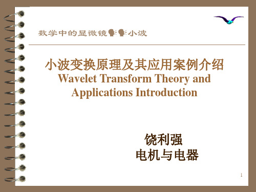
t b )dt a
可见,连续小波变换的结果可以表示为平移因子a和伸 缩因子b的函数
20
3.小波变换的基本原理与性质——多分辨 分析
FT
信号
连续正弦波或余弦波
傅立叶分解过程
CWT
信号
不同尺度和平移因子的小波
小波分解过程
21
3.小波变换的基本原理与性质——多分辨 分析
伸缩因子对小波的作用
2.小波变换与傅里叶变换的比较
(1)克服第一个不足:小波系数不仅像傅立叶系 数那样,是随频率不同而变化的,而且对于同一个频 率指标j, 在不同时刻 k,小波系数也是不同的。 (2)克服第二个不足:由于小波函数具有紧支撑 的性质即某一区间外为零。这样在求各频率水平不同 时刻的小波系数时,只用到该时刻附近的局部信息。 从而克服了上面所述的第二个不足。 (3)克服第三个不足:通过与加窗傅立叶变换的 “时间—频率窗”的相似分析,可得到小波变换的 “时间—频率窗”的笛卡儿积。小波变换的“时间--频 率窗”的宽度,检测高频信号时变窄,检测低频信号 时变宽。这正是时间--频率分析所希望的。根据小波变 换的 “时间—频率窗” 的宽度可变的特点,为了克服 上面所述的第三个不足,只要不同时检测高频与低频 8 信息,问题就迎刃而解了。
24
3.小波变换的基本原理与性质——多分辨 分析
25
3.小波变换的基本原理与性质——多分辨 分析
小波逆变换 如果小波函数满足“容许”条件,那么连续小波变换 的逆变换是存在的
1 x(t ) C
1 C
0
CWTf (a, b) a ,b (t )
1 波变换与傅里叶变换的比较
小波分析是在傅里叶分析的基础上发展起来的, 但小波分析与傅里叶分析存在着极大的不同,与 Fourier变换相比,小波变换是空间(时间)和频率的 局部变换,因而能有效地从信号中提取信息。通过伸 缩和平移等运算功能可对函数或信号进行多尺度的细 化分析,解决了Fourier变换不能解决的许多困难问题。 小波变换联系了应用数学、物理学、计算机科学、信 号与信息处理、图像处理、地震勘探等多个学科。
顺序形态滤波与样本熵在转子故障特征提取中的应用
张文斌
ZHANG W e n . b i n
Байду номын сангаас
( 红河学院 工 学院,蒙 自 6 6 1 1 O 0 )
摘
要 :结合顺序形态滤波方法 与非 线性动力学参数样本熵 , 提 出一种新的转子故障特征提取方法 。首 先引入 循环统 计学 的思 想对传 统形态滤 波方 法进行 改进 ,定 义了顺序 形态滤 波器 ,并 结合实 际选用 最简单 的直线结 构元素 ,对实测 转子 振动信号 进行顺序 形态滤 波降噪预 处理 ;然后计 算降 噪后信号 的样本熵 ,包括 转子正 常 、不 平衡 、不 对中 、油膜涡动 和碰摩 等五种工 况的振 动信号 ;最后将 样本熵 作为特征 ,依 据不 同的故障对应 不 同的样本熵 分布 ,对各种故 障状态 进行评价 . 转子系统故障识别的实例验证 了该方法的可行性和有效性 。
号 ,结 构 元素 的长 度取3 。
‘
B )
显 然 ,样 本熵 的值 与参 数 I T I 和r 的取 值 有 关 。
参 考 文献 [ 4 1 关 于 参数 I T I 和r 不 同取 值 对 样 本熵 的影 响 ,对 实 际转子 振动 信号 估计 样本 熵时 ,取m= 2 和 r = 0 . 2 进行 计算 。
量 的 噪 声干 扰 而 无 法 准 确 反 映 故 障 特 征 的 问 题 ,
基于Morlet小波变换的自适应小波脊线提取算法

Self--adaptive W avelet·-ridge Extraction Algorithm Based on M orlet W avelet Transform
LI Cong,LI W ei (Research Institute of Electronic Science and Technology, University of Electronic Science and Technology of China,Chengdu 61 173 1,China)
order to aajust the shape parameter of M orlet wavelet.which makes the wavelet basis function change in real—time to
adapt to a variety of situations.Sim ulation results show that wavelet—ridge of all kinds of signals can be accurately extracted with the same initial parameter settings.M eanwhile,the new algorithm has a higher probability of detection and noise suppression com pared with the original wavelet ridge extraction algorithm .
中 文 引 用 格 式 :黎 聪 ,李 炜 .基 于 Morlet小 波变 换 的 自适应 小波脊 线提 取算 法 [J].计算机 工程 ,2016,42(4):60·64. 英 文 引 用 格 式 :Li Cong,Li Wei.Self—adaptive Wavelet-ridge Extraction Algorithm Based on Morlet Wavelet Transform[J] Computer Engineer ing,2016,42(4):60—64.
一维横场伊辛模型的精确解

一维横场伊辛模型的精确解伊辛模型是一个最简单且可以提供非常丰富的物理内容的模型,可用于描述很多物理现象,如:合金中的有序-无序转变、液氦到超流态的转变、液体的冻结与蒸发、玻璃物质的性质、森林火灾、城市交通等。
Ising模型的提出最初是为了解释铁磁物质的相变,即磁铁在加热到一定临界温度以上会出现磁性消失的现象,而降温到临界温度以下又会表现出磁性。
这种有磁性、无磁性两相之间的转变,是一种连续相变(也叫二级相变)。
Ising模型假设铁磁物质是由一堆规则排列的小磁针构成,每个磁针只有上下两个方向(自旋)。
相邻的小磁针之间通过能量约束发生相互作用,同时又会由于环境热噪声的干扰而发生磁性的随机转变(上变为下或反之)。
涨落的大小由关键的温度参数决定,温度越高,随机涨落干扰越强,小磁针越容易发生无序而剧烈地状态转变,从而让上下两个方向的磁性相互抵消,整个系统消失磁性,如果温度很低,则小磁针相对宁静,系统处于能量约束高的状态,大量的小磁针方向一致,铁磁系统展现出磁性。
为了研究我们上面所定义的动力学相变,我们要对一维横场伊辛模型的动力学进行求解。
事实上,对于一维横场伊辛模型确实是有精确解的。
早在1925年伊辛就解决了一维伊辛问题。
文章发表初期,引用很少,其中最重要的可能是海森堡1928年论文引言中,引用伊辛经典模型中没有相变,作为引入量子模型的论据。
海森堡模型所引发的统计模型和可积系统的研究,至今方兴未艾、硕果累累。
1944年Onsager发表了平面正方二维伊辛模型的精确解,证明确有一个相变点。
这是统计物理发展的里程碑。
不过那篇文章及其晦涩难懂。
直到1949年Onsager和Kaufmann发表了使用旋子代数的新解法,人们才得以领会奥妙,计算其它晶格,并且开始了求解三维伊辛模型的尝试。
2.1 伊辛模型量子伊辛模型的普遍表达式可以写为[5]:H=−Jg∑σi xi −J∑σi zi,jσj z上述式子的意义:其中J>0,是一个决定微观能量尺度的相互作用常数;g>0,是一个无量纲的耦合常数,被用来调节H跨过量子相变点。
第2部分多媒体技术基础精品文档

(4) 1980: Morlet提出了CWT
CWT (continuous wavelet transform) 20世纪70年代,当时在法国石油公司工作
的年轻的地球物理学家Jean Morlet提出了 小波变换WT(wavelet transform)的概念。 20世纪80年代,从STFT开发了CWT:
1. What is wavelet
一种函数
具有有限的持续时间、突变的频率和振幅 波形可以是不规则的,也可以是不对称的 在整个时间范围里的幅度平均值为零 比较正弦波
部分小波波形
小波的定义
Wavelets are a class of a functions used to localize a given function in both space and scaling. A family of wavelets can be constructed from a ( x ) function , sometimes known as a "mother wavelet," which is confined in a finite interval. "Daughter wavelets" (a,b) ( x ) are then formed by translation (b) and contraction (a). Wavelets are especially useful for compressing image data, since a wavelet transform has properties which are in some ways superior to a conventional Fourier transform.
小波变换名词解释

小波变换名词解释
小波变换(Wavelet Transformer)是一种基于矩阵分解和线性代数运算的数学工具,用于将高维数据映射到低维空间中,同时保留数
据中的模式和特征。
小波变换主要分为三种类型:小波基(Waveletzeros)、小波函数(Wavelet Functions)和小波样条函数(Wavelet Series Function)。
小波基是一种离散化的高维数据,小波函数和小波样条函数则是用高维数据表示的线性变换。
小波变换可以通过矩阵分解的方式实现,将高维数据映射到低维空间中,同时保留数据中的模式和特征。
在这个过程中,矩阵分解和线性代数运算是必不可少的。
小波变换广泛应用于信号处理、图像处理、模式识别、计算机视觉等领域。
它可以提取数据中的高频和低频分量,从而实现对数据的分析和理解。
基于相空间重构的神经网络风暴潮增水预测方法
基于相空间重构的神经网络风暴潮增水预测方法尤成;于福江;原野【摘要】风暴潮增水的准确预测对于国民生产、防灾减灾有重大意义.本文提出一种基于相空间重构的神经网络风暴潮增水预测方法,即使用单站风暴潮增水数据重构出与之相关的相空间,然后使用BP神经网络模型拟合该相空间的空间结构.将该模型用于库克斯港风暴潮增水预测,结果表明:该模型应用在风暴潮增水时间序列的预测中是合理、可行的,并具有较高的精度.此外,使用dbl0小波函数对原始余水位数据进行降噪处理可以显著地提高模型的预测精度.【期刊名称】《海洋预报》【年(卷),期】2016(033)001【总页数】6页(P59-64)【关键词】相空间重构;BP神经网络;风暴潮增水预测;小波降噪【作者】尤成;于福江;原野【作者单位】国家海洋环境预报中心国家海洋局海洋灾害预报技术研究重点实验室,北京100081;国家海洋环境预报中心国家海洋局海洋灾害预报技术研究重点实验室,北京100081;国家海洋环境预报中心国家海洋局海洋灾害预报技术研究重点实验室,北京100081【正文语种】中文【中图分类】P731.23Packard等[1]提出了重构相空间的思想。
随后Takens等[2]提出嵌入定理,建立起观测资料与动力系统空间特征之间的桥梁,使得深入分析时间序列的背景和动力学机制成为可能。
Lyapunov指数、G-P关联维算法、虚假近邻法、Cao方法、自相关法、互信息法、C-C方法等对各种参数的计算,使得相空间重构技术日趋成熟。
Farmer等[3]第一次提出使用相空间重构的方法预测时间序列。
这个方法后来被称作k-NN方法。
许多学者讨论K-NN方法中权重系数ωi该如何取值[4-6]。
为了尽量避免k的选取引起预测误差,Yankov等[7]以一组k取值不同的k-NN方法为成员,进行集合预报,发现预报效果有一定的改进。
此外,人们在天气预报、水文预报等方面应用相空间重构的理论进行了研究取得了相当的成果。
关于声波逆散射问题的factorization方法
关于声波逆散射问题的factorization方法声波逆散射问题是经典的反问题之一,其主要目的是通过接收到的散射波来确定散射体的形状和位置信息。
而factorization方法则是其中一种有效的求解手段。
下面将从数学、物理和工程应用等方面分别探讨该方法的原理及其优缺点。
一、数学层面Factorization方法的核心理念在于将散射反问题转化为数学解析问题。
其基本步骤是首先通过多极子展开表示出体散射的入射场和散射场,然后运用因子化技术将一个矩阵分解成两个矩阵的乘积,从而实现了对入射场和散射场的有效解耦。
此外,该方法还能利用希尔伯特空间中的正交基和Fréchet导数等数学工具进行求解,从而更进一步提高了计算精度和效率。
二、物理层面Factorization方法的物理意义在于探明了体散射的本质特点,即每个不同的体散射都可以通过一个自由空间内的多极子散射体进行模拟。
因此,如果我们能够得到一个准确的入射场和散射场,就可以推导出体散射的形状、大小甚至材料性质。
但是,factorization方法在实际应用中存在一些限制。
例如,如果对于同一入射场,存在多个不同的体散射,那么对应的散射矩阵就无法唯一分解。
此外,如果入射波的频率过高或散射物体的尺寸过小,也容易出现求解不稳定等数值问题。
三、工程应用虽然factorization方法在非线性、多参数等复杂反问题中并不具有普适性,但在某些特定领域如医学影像、无损检测等中广泛应用。
例如,利用人体表面的声波反射和散射信息可以实现心脏、肺部疾病的诊断和检测;在航空航天、地质勘探等工程领域,也可以通过声波逆散射技术对结构物的材料损伤、地下矿脉、油气开采等进行无损探测和监测。
总的来说,factorization方法作为声波逆散射问题的一种有效求解手段,其数学基础和物理本质十分重要。
虽然在实际工程应用中可能存在一些局限性和缺陷,但其精准和高效的计算特性,使其在特定领域中得到了广泛的应用和推广。
- 1、下载文档前请自行甄别文档内容的完整性,平台不提供额外的编辑、内容补充、找答案等附加服务。
- 2、"仅部分预览"的文档,不可在线预览部分如存在完整性等问题,可反馈申请退款(可完整预览的文档不适用该条件!)。
- 3、如文档侵犯您的权益,请联系客服反馈,我们会尽快为您处理(人工客服工作时间:9:00-18:30)。
FACTORING W A VELET TRANSFORMS INTO LIFTING STEPSINGRID DAUBECHIES AND WIM SWELDENSSeptember1996,revised November1997A BSTRACT.This paper is essentially tutorial in nature.We show how any discrete wavelet transform ortwo band subbandfiltering withfinitefilters can be decomposed into afinite sequence of simplefilter-ing steps,which we call lifting steps but that are also known as ladder structures.This decompositioncorresponds to a factorization of the polyphase matrix of the wavelet or subbandfilters into elementarymatrices.That such a factorization is possible is well-known to algebraists(and expressed by the formula);it is also used in linear systems theory in the electrical engineering community.We present here a self-contained derivation,building the decomposition from basic principlessuch as the Euclidean algorithm,with a focus on applying it to waveletfiltering.This factorization providesan alternative for the lattice factorization,with the advantage that it can also be used in the biorthogonal,i.e,non-unitary case.Like the lattice factorization,the decomposition presented here asymptotically re-duces the computational complexity of the transform by a factor two.It has other applications,such as thepossibility of defining a wavelet-like transform that maps integers to integers.1.I NTRODUCTIONOver the last decade several constructions of compactly supported wavelets originated both from mathematical analysis and the signal processing community.The roots of critically sampled wavelet transforms are actually older than the word“wavelet”and go back to the context of subbandfilters,or more precisely quadrature mirrorfilters[35,36,42,50,51,52,53,57,55,59].In mathematical analysis, wavelets were defined as translates and dilates of onefixed function and were used to both analyze and represent general functions[13,18,22,34,21].In the mid eighties the introduction of multiresolution analysis and the fast wavelet transform by Mallat and Meyer provided the connection between subband filters and wavelets[30,31,34];this led to new constructions,such as the smooth orthogonal,and com-pactly supported wavelets[16].Later many generalizations to the biorthogonal or semiorthogonal(pre-wavelet)case were introduced.Biorthogonality allows the construction of symmetric wavelets and thus linear phasefilters.Examples are:the construction of semiorthogonal spline wavelets[1,8,10,11,49], fully biorthogonal compactly supported wavelets[12,56],and recursivefilter banks[25].Various techniques to construct wavelet bases,or to factor existing waveletfilters into basic building blocks are known.One of these is lifting.The original motivation for developing lifting was to buildsecond generation wavelets,i.e.,wavelets adapted to situations that do not allow translation and dilation like non-Euclidean spaces.First generation wavelets are all translates and dilates of one or a few basic shapes;the Fourier transform is then the crucial tool for wavelet construction.A construction using lifting,on the contrary,is entirely spatial and therefore ideally suited for building second generation wavelets when Fourier techniques are no longer available.When restricted to the translation and dilation invariant case,or the“first generation,”lifting comes down to well-known ladder type structures and certain factoring algorithms.In the next few paragraphs,we explain lifting and show how it provides a spatial construction and allows for second generation wavelets;later we focus on thefirst generation case and the connections with factoring schemes.The basic idea of wavelet transforms is to exploit the correlation structure present in most real life sig-nals to build a sparse approximation.The correlation structure is typically local in space(time)and fre-quency;neighboring samples and frequencies are more correlated than ones that are far apart.Traditional wavelet constructions use the Fourier transform to build the space-frequency localization.However,as the following simple example shows,this can also be done in the spatial domain.Consider a signal with.Let us split it in two disjoint sets which are called the polyphase components:the even indexed samples,or“evens”for short,and the odd indexed samples,or“odds.”Typically these two sets are closely correlated.Thus it is only natural that given one set,e.g.,the odd,one can build a good predictor for the other set,e.g.,the even.Of course the predictor need not be exact,so we need to record the difference or detail:Given the detail and the odd,we can immediately recover the odd asIf is a good predictor,then approximately will be a sparse set;in other words,we expect thefirst order entropy to be smaller for than for.Let us look at a simple example.An easy predictor for an odd sample is simply the average of its two even neighbors;the detail coefficient then isFrom this we see that if the original signal is locally linear,the detail coefficient is zero.The operation of computing a prediction and recording the detail we will call a lifting step.The idea of retaining rather than is well known and forms the basis of so-called DPCM methods[26,27].This idea connects naturally with wavelets as follows.The prediction steps can take care of some of the spatial correlation, but for wavelets we also want to get some separation in the frequency domain.Right now we have a transform from to.The frequency separation is poor since is obtained by simply subsampling so that serious aliasing occurs.In particular,the running average of the is not the same as that of the original samples.To correct this,we propose a second lifting step,which replaces the2evens with smoothed values with the use of an update operator applied to the details:Again this step is trivially invertible:given we can recover asand then can be recovered as explained earlier.This illustrates one of the built-in features of lifting: no matter how and are chosen,the scheme is always invertible and thus leads to critically sampled perfect reconstructionfilter banks.The block diagram of the two lifting steps is given in Figure1.F IGURE1.Block diagram of predict and update lifting steps.Coming back to our simple example,it is easy to see that an update operator that restores the correct running average,and therefore reduces aliasing,is given byThis can be verified graphically by looking at Figure2.This simple example,when put in the wavelet framework,turns out to correspond to the biorthogonal (2,2)wavelet transform of[12],which was originally constructed using Fourier arguments.By the construction above,which did not use the Fourier transform but instead reasoned using only spatial arguments,one can easily work in a more general setting.Imagine for a moment that the samples were irregularly ing the same spatial arguments as above we could then see that a good predictor is of the form where the varies spatially and depends on the irregularity of the grid.Similarly spatially varying update coefficients can be computed[46].This thus immediately allows for a(2,2)type transform for irregular samples.These spatial lifting steps can also be used in higher dimensions(see[45])and leads e.g.,to wavelets on a sphere[40]or more complex manifolds.Note that the idea of using spatial wavelet constructions for building second generation wavelets has been proposed by several researchers:The lifting scheme is inspired by the work of Donoho[19]and Lounsbery et al.[29].Donoho[19] shows how to build wavelets from interpolating scaling functions,while Lounsbery et al.build a multiresolution analysis of surfaces using a technique that is algebraically the same as lifting.3F IGURE2.Geometric interpretation for piecewise linear predict and update liftingsteps.The original signal is drawn in bold.The wavelet coefficient is computedas the difference of an odd sample and the average of the two neighboring evens.Thiscorresponds to a loss in area drawn in grey.To preserve the running average thisarea has to be redistributed to the even locations resulting in a coarser piecewise linearsignal drawn in thin line.Because the coarse scale is twice thefine scale and twoeven locations are affected,,i.e,one quarter of the wavelet coefficient,has to beadded to the even samples to obtain the.Then the thin and bold lines cover the samearea.(For simplicity we assumed that the wavelet coefficients and are zero.)Dahmen and collaborators,independently of lifting,worked on stable completions of multiscale transforms,a setting similar to second generation wavelets[7,15].Again independently,both of Dahmen and of lifting,Harten developed a general multiresolution approximation framework based on spatial prediction[23].In[14],Dahmen and Micchelli propose a construction of compactly supported wavelets that gen-erates complementary spaces in a multiresolution analysis of univariate irregular knot splines. The construction of the(2,2)example via lifting is one example of a2step lifting construction for an entire family of Deslauriers-Dubuc biorthogonal interpolating wavelets.Lifting thus provides a frame-work that allows the construction of certain biorthogonal wavelets which can be generalized to the second generation setting.A natural question now is how much of thefirst generation wavelet families can be built with the lifting framework.It turns out that every FIR wavelet orfilter bank can be decomposed into lifting steps.This can be seen by writing the transform in the polyphase form.Statements concerning perfect reconstruction or lifting can then be made using matrices with polynomial or Laurent polynomial entries.A lifting step then becomes a so-called elementary matrix,that is,a triangular matrix(lower or upper)with all diagonal entries equal to one.It is a well known result in matrix algebra that any matrixwith polynomial entries and determinant one can be factored into such elementary matrices.For those familiar with the common notation in thisfield,this is written as. The proof relies on the2000year old Euclidean algorithm.In thefilter bank literature subband transform built using elementary matrices are known as ladder structures and were introduced in[5].Later several constructions concerning factoring into ladder steps were given[28,41,48,32,33].Vetterli and Herley [56]also use the Euclidean algorithm and the connection to diophantine equations tofind all high pass filters that,together with a given low-passfilter,make afinitefilter wavelet transform.Van Dyck et al. use ladder structures to design a wavelet video coder[20].In this paper we give a self-contained constructive proof of the standard factorization result and apply it to several popular wavelets.We consider the Laurent polynomial setting as opposed to the standard polynomial setting because it is more general,allows for symmetry and also poses some interesting questions concerning non-uniqueness.This paper is organized as follows.In Section2we review some facts aboutfilters and Laurent polynomials.Section3gives the basics behind wavelet transforms and the polyphase representation while Section4discusses the lifting scheme.We review the Euclidean algorithm in Section5before moving to the main factoring result in Section6.Section7gives several examples.In Section8we show how lifting can reduce the computational complexity of the wavelet transform by a factor two.Finally Section9contains comments.2.F ILTERS AND L AURENT POLYNOMIALSAfilter is a linear time invariant operator and is completely determined by its impulse response: .Thefilter is a Finite Impulse Response(FIR)filter in case only afinite number of filter coefficients are non-zero.We then let(respectively)be the smallest(respectively largest) integer number for which is non-zero.The-transform of a FIRfilter is a Laurent polynomial given byIn this paper,we consider only FIRfilters.We often use the symbol to denote both thefilter and the associated Laurent polynomial.The degree of a Laurent polynomial is defined asSo the length of thefilter is the degree of the associated polynomial plus one.Note that the polynomial seen as a Laurent polynomial has degree zero,while as a regular polynomial it would have degree. In order to make consistent statements,we set the degree of the zero polynomial to.The set of all Laurent polynomials with real coefficients has a commutative ring structure.The sum or difference of two Laurent polynomials is again a Laurent polynomial.The product of a Laurent5polynomial of degree and a Laurent polynomial of degree is a Laurent polynomial of degree. This ring is usually denoted as.Within a ring,exact division is not possible in general.However,for Laurent polynomials,division with remainder is possible.Take two Laurent polynomials and with,then there always exists a Laurent polynomial(the quotient)with,and a Laurent polynomial(the remainder)with so thatWe denote this as(C-language notation):andIf which means is a monomial,then and the division is exact.A Laurent poly-nomial is invertible if and only if it is a monomial.This is the main difference with the ring of(regular) polynomials where constants are the only polynomials that can be inverted.Another difference is that the long division of Laurent polynomials is not necessarily unique.The following example illustrates this.Example1.Suppose we want to divide by.This means we have to find a Laurent polynomial of degree1so that given byis of degree zero.This implies that has to match in two terms.If we let those terms be the term in and the constant then the answer is.Indeed,The remainder thus is of degree zero and we have completed the division.However if we choose the two matching terms to be the ones in and,the answer is.Indeed,Finally,if we choose to match the constant and the term in,the solution is and the remainder is.The fact that division is not unique will turn out to be particularly useful later.In general has to match in at least terms,but we are free to choose these terms in the beginning, the end,or divided between the beginning and the end of.For each choice of terms a corresponding long division algorithm exists.In this paper,we also work with matrices of Laurent polynomials,e.g.,6F IGURE3.Discrete wavelet transform(or subband transform):The forward transformconsists of two analysisfilters(low-pass)and(high-pass)followed by subsampling,while the inverse transformfirst upsamples and then uses two synthesisfilters(low-pass)and(high-pass).These matrices also form a ring,which is denoted by.If the determinant of such a matrix is a monomial,then the matrix is invertible.The set of invertible matrices is denoted.A matrix from this set is unitary(sometimes also referred to as para-unitary)in case3.W AVELET TRANSFORMSFigure3shows the general block scheme of a wavelet or subband transform.The forward transform uses two analysisfilters(low-pass)and(band pass)followed by subsampling,while the inverse transformfirst upsamples and then uses two synthesisfilters(low-pass)and(high-pass).For details on wavelet and subband transforms we refer to[43]and[57].In this paper we consider only the case where the fourfilters,,,and,of the wavelet transform are FIRfilters.The conditions for perfect reconstruction are given byWe define the modulation matrix asWe similarly define the dual modulation matrix.The perfect reconstruction condition can now be written as(1) where is the identity matrix.If allfilters are FIR,then the matrices and belong to .A special case are orthogonal wavelet transforms in which case and.The modulation matrix is thenLP BPandLPBPF IGURE5.The lifting scheme:First a classical subbandfilter scheme and then liftingthe low-pass subband with the help of the high-pass subband.LPBPF IGURE6.The dual lifting scheme:First a classical subbandfilter scheme and laterlifting the high-pass subband with the help of the low-pass subband.The problem offinding an FIR wavelet transform thus amounts tofinding a matrix with deter-minant one.Once we have such a matrix,and the fourfilters for the wavelet transform follow immediately.From(2)and Cramer’s rule it follows thatThis impliesandThe most trivial example of a polyphase matrix is.This results inand.The wavelet transform then does nothing else but subsampling even and odd samples.This transform is called the polyphase transform,but in the context of lifting it is often referred to as the Lazy wavelet transform[44].(The reason is that the notion of the Lazy wavelet can also be used in the second generation setting.)4.T HE L IFTING S CHEMEThe lifting scheme[44,45]is an easy relationship between perfect reconstructionfilter pairsthat have the same low-pass or high-passfilter.One can then start from the Lazy wavelet and use lifting to gradually build one’s way up to a multiresolution analysis with particular properties.Definition2.Afilter pair is complementary in case the corresponding polyphase matrix has determinant1.9If is complementary,so is.This allows us to state the lifting scheme.Theorem3(Lifting).Let be complementary.Then any otherfinitefilter complementary to is of the form:where is a Laurent polynomial.Conversely anyfilter of this form is complementary to. Proof.The polyphase components of are for even and for odd.After lifting,the new polyphase matrix is thus given byThis operation does not change the determinant of the polyphase matrix.Figure5shows the schematic representation of lifting.Theorem3can also be written relating the low-passfilters and.In this formulation,it is exactly the Vetterli-Herley lemma[56,Proposition4.7]. The dual polyphase matrix is given by:We see that lifting creates a newfilter given byTheorem4(Dual lifting).Let be complementary.Then any otherfinitefilter complementary to is of the form:where is a Laurent polynomial.Conversely anyfilter of this form is complementary to.After dual lifting,the new polyphase matrix is given byDual lifting creates a new given byFigure6shows the schematic representation of dual lifting.In[44]lifting and dual lifting are used to build wavelet transforms starting from the Lazy wavelet.There a whole family of wavelets is constructed from the Lazy followed by one dual lifting and one primal lifting step.All thefilters constructed this way are half band and the corresponding scaling functions are interpolating.Because of the many advantages of lifting,it is natural to try to build other wavelets as well,perhaps using multiple lifting10steps.In the next section we will show that any wavelet transform withfinitefilters can be obtained starting from the Lazy followed by afinite number of alternating lifting and dual lifting steps.In order to prove this,wefirst need to study the Euclidean algorithm in closer detail.5.T HE E UCLIDEAN A LGORITHMThe Euclidean algorithm was originally developed tofind the greatest common divisor of two natural numbers,but it can be extended tofind the greatest common divisor of two polynomials,see,e.g,[4]. Here we need it tofind common factors of Laurent polynomials.The main difference with the polynomial case is again that the solution is not unique.Indeed the gcd of two Laurent polynomials is defined only up to a factor.(This is similar to saying that the gcd of two polynomials is defined only up to a constant.) Two Laurent polynomials are relatively prime in case their gcd has degree zero.Note that they can share roots at zero and infinity.Theorem5(Euclidean Algorithm for Laurent Polynomials).Take two Laurent polynomials and with Let and and iterate the following steps starting from(3)(4) Then where is the smallest number for which.Given that,there is an so that.The algorithm thenfinishes for .The number of steps thus is bounded by.If we let, we have thatConsequentlyand thus divides both and.If is a monomial,then and are relatively prime.Example6.Let and.Then thefirst division gives us(see the example in Section2):11The next step yieldsThus,and are relatively prime andThe number of steps here is.6.T HE F ACTORING A LGORITHMIn this section,we explain how any pair of complementaryfilters can be factored into lifting steps.First,note that and have to be relatively prime because any common factor would also divide and we already know that is1.We can thus run the Euclidean algorithm starting from and and the gcd will be a monomial.Given the non-uniqueness of the division we can always choose the quotients so that the gcd is a constant.Let this constant be.We thus have thatNote that in case,thefirst quotient is zero.We can always assume that is even. Indeed if is odd,we can multiply thefilter with and with.This does not change the determinant of the polyphase matrix.Itflips(up to a monomial)the polyphase components of and thus makes even again.Given afilter we can alwaysfind a complementaryfilter by lettingHere thefinal diagonal matrix follows from the fact that the determinant of a polyphase matrix is one and is even.Let us slightly rewrite the last equation.First observe that(5) Using thefirst equation of(5)in case is odd and the second in case is even yields:(6) Finally,the originalfilter can be recovered by applying Theorem3.12Now we know that thefilter can always be obtained from with one lifting or:(7) Combining all these observations we now have shown the following theorem:Theorem7.Given a complementaryfilter pair,then there always exist Laurent polynomials and for and a non-zero constant so thatThe proof follows from combining(6)and(7),setting,,and .In other words everyfinitefilter wavelet transform can be obtained by starting with the Lazy wavelet followed by lifting and dual lifting steps followed with a scaling.The dual polyphase matrix is given byFrom this we see that in the orthogonal case()we immediately have two different factor-izations.Figures7and8represent the different steps of the forward and inverse transform schematically.7.E XAMPLESWe start with a few easy examples.We denotefilters either by their canonical names(e.g.Haar),by ()where(resp.)is the number of vanishing moments of(resp.),or by where is the length of analysisfilter and is the length of the synthesisfilter.We start with a sequence and denote the result of applying the low-passfilter(resp.high-passfilter)and downsampling as a sequence(resp.).The intermediate values computed during lifting we denote with sequences and.All transforms are instances of Figure7.7.1.Haar wavelets.In the case of(unnormalized)Haar wavelets we have that,,,ing the Euclidean algorithm we can thus write the polyphase matrix as:Thus on the analysis size we have:13LPBPF IGURE7.The forward wavelet transform using lifting:First the Lazy wavelet,thenalternating lifting and dual lifting steps,andfinally a scaling.LPBPWe can also do it without scaling with three lifting steps as(here assuming)This corresponds to the well known fact in geometry that a rotation can always be written as three shears. The lattice factorization of[51]allows the decomposition of any orthonormalfilter pair into shifts and Givens rotations.It follows that any orthonormalfilter can be written as lifting steps,byfirst writing the lattice factorization and then using the example above.This provides a different proof of Theorem7in the orthonormal case.7.3.Scaling.These two examples show that the scaling from Theorem7can be replaced with four lifting steps:orGiven that one can always merge one of the four lifting steps with the last lifting step from the factor-ization,only three extra steps are needed to avoid scaling.This is particularly important when building integer to integer wavelet transforms in which case scaling is not invertible[6].7.4.Interpolatingfilters.In case the low-passfilter is half band,or,the correspond-ing scaling function is interpolating.Since,the factorization can be done in two steps:Thefilters constructed in[44]are of this type.This gives rise to a family of(and even) symmetric biorthogonal wavelets built from the Deslauriers–Dubuc scaling functions mentioned in the introduction.The degrees of thefilters are and.In case,these are particularly easy as.(Beware:the normalization used here is different from the one in[44].)Next we look at some examples that had not been decomposed into lifting steps before.7.5.4-tap orthonormalfilter with two vanishing moments(D4).Here the andfilters are given by [16]:15withThe polyphase matrix is(8) and the factorization is given by:This corresponds to the following implementation for the forward transform:16The other option is to use(9)as a factorization for.The analysis polyphase matrix then is factored as:Given that the inverse transform always follows immediately from the forward transform,from now on we only give the forward transform.One can also obtain an entirely different lifting factorization of D4by shifting thefilter pair corre-sponding to:withas polyphase matrix.This leads to a different factorization:17This second factorization can also be obtained as the result of seeking a factorization of the original polyphase matrix(8)where thefinal diagonal matrix has(non-constant)monomial entries.7.6.6-tap orthonormalfilter with three vanishing moments(D6).Here we havewith[16]The polyphase components areIn the factorization algorithm the coefficients of the remainders are calculated as:If we now letthen the factorization is given by:18We leave the implementation of thisfilter as an exercise for the reader.7.7.(9-7)filter.Here we consider the popular(9-7)filter pair.The analysisfilter has9coefficients, while the synthesisfilter has7coefficients.Both high-passfilters and have4vanishing moments. We choose thefilter with7coefficients to be the synthesisfilter because it gives rises to a smoother scaling function than the9coefficient one(see[17,p.279,Table8.3],note that the coefficients need to be multiplied withThe factorization leads to the following implementation:7.8.Cubic B-splines.Wefinish with an example that is used frequently in computer graphics:the(4,2) biorthogonalfilter from[12].The scaling function here is a cubic B-spline.This example can be obtained again by using the factoring algorithm.However,there is also a much more intuitive construction in the spatial domain[46].Thefilters are given byand the factorization reads:8.C OMPUTATIONAL COMPLEXITYIn this section we take a closer look at the computational complexity of the wavelet transform com-puted using lifting.As a comparison base we use the standard algorithm,which corresponds to applying the polyphase matrix.This already takes advantage of the fact that thefilters will be subsampled and thus avoids computing samples that will be subsampled immediately.The unit we use is the cost,mea-sured in number of multiplications and additions,of computing one sample pair.The cost of applying afilter is multiplications and additions.The cost of the standard algorithm thus is .If thefilter is symmetric and is even,the cost is.Let us consider a general case not involving symmetry.Take,,and assume.The cost of the standard algorithm now is.Without loss of generality we can assume that,,,and.In general the Euclidean algorithm started from the pair now needs steps with the degree of each quotient equal to one(for ).To get the pair,one extra lifting step(7)is needed with.The total cost of the20lifting algorithm is:scaling:lifting steps:final lifting step:Wavelet Standard Lifting SpeedupT putational cost of lifting versus the standard algorithm.Asymptoticallythe lifting algorithm is twice as fast as the standard algorithm.One has to be careful with this comparison.Even though it is widely used,the standard algorithm is not necessarily the best way to implement the wavelet transform.Lifting is only one idea in a whole tool bag of methods to improve the speed of a fast wavelet transform.Rioul and Duhamel[39]discuss several other schemes to improve the standard algorithm.In the case of longfilters,they suggest an FFT based scheme known as the Vetterli-algorithm[56].In the case of shortfilters,they suggest a“fast running FIR”algorithm[54].How these ideas combine with the idea of using lifting and which combination will be optimal for a certain wavelet goes beyond the scope of this paper and remains a topic of future research.21。
