Bounds for the chromatic number of graphs with partial information
算法分析与设计基础答案11章
This file contains the exercises, hints, and solutions for Chapter 11 of the book ”Introduction to the Design and Analysis of Algorithms,” 3rd edition, by A. Levitin. The problems that might be challenging for at least some students are marked by B; those that might be difficult for a majority of students are marked by I
J. Comput. Chem.
2D Depiction of Nonbonding Interactions forProtein ComplexesPENG ZHOU,1FEIFEI TIAN,2ZHICAI SHANG11Institute of Molecular Design&Molecular Thermodynamics,Department of Chemistry,Zhejiang University,Hangzhou310027,China2College of Bioengineering,Chongqing University,Chongqing400044,ChinaReceived7May2008;Revised25June2008;Accepted22July2008DOI10.1002/jcc.21109Published online22October2008in Wiley InterScience().Abstract:A program called the2D-GraLab is described for automatically generating schematic representation of nonbonding interactions across the protein binding interfaces.The inputfile of this program takes the standard PDB format,and the outputs are two-dimensional PostScript diagrams giving intuitive and informative description of the protein–protein interactions and their energetics properties,including hydrogen bond,salt bridge,van der Waals interaction,hydrophobic contact,p–p stacking,disulfide bond,desolvation effect,and loss of conformational en-tropy.To ensure these interaction information are determined accurately and reliably,methods and standalone pro-grams employed in the2D-GraLab are all widely used in the chemistry and biology community.The generated dia-grams allow intuitive visualization of the interaction mode and binding specificity between two subunits in protein complexes,and by providing information on nonbonding energetics and geometric characteristics,the program offers the possibility of comparing different protein binding profiles in a detailed,objective,and quantitative manner.We expect that this2D molecular graphics tool could be useful for the experimentalists and theoreticians interested in protein structure and protein engineering.q2008Wiley Periodicals,Inc.J Comput Chem30:940–951,2009Key words:protein–protein interaction;nonbonding energetics;molecular graphics;PostScript;2D-GraLabIntroductionProtein–protein recognition and association play crucial roles in signal transduction and many other key biological processes. Although numerous studies have addressed protein–protein inter-actions(PPIs),the principles governing PPIs are not fully under-stood.1,2The ready availability of structural data for protein complexes,both from experimental determination,such as by X-ray crystallography,and by theoretical modeling,such as protein docking,has made it necessary tofind ways to easily interpret the results.For that,molecular graphics tools are usually employed to serve this purpose.3Although a large number of software packages are available for visualizing the three-dimen-sional(3D)structures(e.g.PyMOL,4GRASP,5VMD,6etc.)and interaction modes(e.g.MolSurfer,7ProSAT,8PIPSA,9etc.)of biomolecules,the options for producing the schematic two-dimensional(2D)representation of nonbonding interactions for PPIs are very scarce.Nevertheless,a few2D graphics programs were developed to depict protein-small ligand interactions(e.g., LIGPLOT,10PoseView,11MOE,12etc.).These tools,however, are incapable of handling the macromolecular complexes.Some other available tools presenting macromolecular interactions in 2D level mainly include DIMPLOT,10NUCPLOT,13and MON-STER,14etc.Amongst,only the DIMPLOT can be used for aesthetically visualizing the nonbinding interactions of PPIs. However,such a program merely provides a simple description of hydrogen bonds,hydrophobic interactions,and steric clashes across the binding interfaces.In this article,we describe a new molecular graphics tool, called the two-dimensional graphics lab for biosystem interac-tions(2D-GraLab),which adopts the page description language (PDL)to intuitively,exactly,and detailedly reproduce the non-bonding interactions and energetics properties of PPIs in Post-Script page.Here,the following three points are the emphasis of the2D-GraLab:(i)Reliability.To ensure the reliability,the pro-grams and methods employed in2D-GraLab are all widely used in chemistry and biology community;(ii)Comprehensiveness. 2D-GraLab is capable of handling almost all the nonbonding interactions(and even covalent interactions)across binding Additional Supporting Information may be found in the online version of this article.Correspondence to:Z.Shang;e-mail:shangzc@interface of protein complexes,such as hydrogen bond,salt bridge,van der Waals(vdW)interaction,hydrophobic contact, p–p stacking,disulfide bond,desolvation effect,and loss of con-formational entropy.The outputted diagrams are diversiform, including individual schematic diagram and summarized sche-matic diagram;(iii)Artistry.We elaborately scheme the layout, color match,and page style for different diagrams,with the goal of producing aesthetically pleasing2D images of PPIs.In addi-tion,2D-GraLab provides a graphical user interface(GUI), which allows users to interact with this program and displays the spatial structure and interfacial feature of protein complexes (see .Fig.S1).Identifying Protein Binding InterfacesAn essential step in understanding the molecular basis of PPIs is the accurate identification of interprotein contacts,and based upon that,subsequent works are performed for analysis and lay-out of nonbonding mon methods identifyingprotein–protein binding interfaces include a Voronoi polyhedra-based approach,changes in solvent accessible surface area(D SASA),and various radial cutoffs(e.g.,closest atom,C b,andcentroid,etc.).152D-GraLab allows for the identification of pro-tein–protein binding interfaces at residue and atom levels.Identifying Binding Interfaces at Residue LevelAll the identifying interface methods at residue level belong toradial cutoff approach.In the radial cutoff approach,referencepoint is defined in advance for each residue,and the residues areconsidered in contact if their reference points fell within thedefined cutoff ually,the C a,C b,or centroid are usedas reference point.16–18In2D-GraLab,cutoff distance is moreflexible:cutoff distance5r A1r B1d,where r A and r B are residue radii and d is set by users(as the default d54A˚,which was suggested by Cootes et al.19).Identifying Binding Interfaces at Atom LevelAt atom level,binding interfaces are identified using closestatom-based radial cutoff approach20and D SASA-basedapproach.21For the closest atom-based radial cutoff approach,ifthe distance between any two atoms of two residues from differ-ent chains is less than a cutoff value,the residues are consideredin contact;In the D SASA-based approach,the SASA is calcu-lated twice to identify residues involved in a binding interface,once for the monomers and once for the complex,if there is achange in the SASA(D SASA)of a residue when going from themonomers to the dimer form,then it is considered involved inthe binding interface.In2D-GraLab,three manners are provided for visualizing thebinding interfaces,including spatial structure exhibition,residuedistance plot,and residue-pair contact map(see .Figs.S2–S4).Analysis and2D Layout of NonbondingInteractionsThe inputfile of2D-GraLab is standard PDB format,and the outputs are two-dimensional PostScriptfile giving intuitive and informative representation of the PPIs and their strengths, including hydrogen bond,salt bridge,vdW interaction,desolva-tion effect,ion-pair,side-chain conformational entropy(SCE), etc.The outputs are in two forms as individual schematic dia-gram and summarized schematic diagram.The individual sche-matic diagram is a detailed depiction of each nonbonding profile,whereas the summarized schematic diagram covers all nonbonding interactions and disulfide bonds across the binding interface.To produce the aesthetically high quality layouts,which pos-sess reliable and accurate parameters,several widely used pro-grams listed in Table1are employed in2D-GraLab to perform the core calculations and analysis of different nonbonding inter-actions.2D-GraLab carries out prechecking procedure for pro-tein structures and warns the structural errors,but not providing revision and refinement functions.Therefore,prior to2D-GraLab analysis,protein structures are strongly suggested to be prepro-cessed by programs such as PROCHECK(structure valida-tion),27Scwrl3(side-chain repair),28and X-PLOR(structure refinement).29Individual Schematic DiagramHydrogen BondThe program we use for analyzing hydrogen bonds across bind-ing interfaces is HBplus,23which calculates all possible posi-tions for hydrogen atoms attached to donor atoms which satisfy specified geometrical criteria with acceptor atoms in the vicinity. In2D-GraLab,users can freely select desired hydrogen bonds involving N,O,and/or S atoms.Besides,the water-mediated hydrogen bond is also given consideration.Bond strength of conventional hydrogen bonds(except those of water-mediated Table1.Standalone Programs Employed in2D-GraLab.Program FunctionReduce v3.0322Adding hydrogen atoms for proteinsHBplus v3.1523Identifying hydrogen bonds and calculatingtheir geometric parametersProbe v2.1224Identifying steric contacts and clashes at atomlevelMSMS v2.6125Calculating SASA values of protein atoms andresiduesDelphi v4.026Calculating Coulombic energy and reactionfield energy,determining electrostatic energyof ion-pairsDIMPLOT v4.110Providing application programming interface,users can directly set and executeDIMPLOT in the2D-GraLab GUI9412D Depiction of Nonbonding Interactions for Protein ComplexesFigure1.(a)Schematic representation of a conventional hydrogen bond and a water-mediated hydro-gen bond across the binding interface of IGFBP/IGF complex(PDB entry:2dsr).This diagram was produced using2D-Gralab.The conventional hydrogen bond is formed between the atom N(at the backbone of residue Leu69in chain B)and the atom OE1(at the side-chain of residue Glu3in chain I);The water-mediated hydrogen bond is formed between the atom ND1(at the side-chain of residue His5in chain B)and the atom O(at the backbone of residue Asp20in chain I),and because hydrogen positions of water are almost never known in the PDBfile,the water molecule,when serving as hydrogen bond donor,is not yet determined for its H...A length and D—H...A angle,denoted as mark ‘‘????.’’In this diagram,chains,residues,and atoms are labeled according to the PDB format.(b)Spa-tial conformation of the conventional hydrogen bond.(c)Spatial conformation of the water-mediated hydrogen bond.hydrogen bonds)is calculated using Lennard-Jones 8-6potential with angle weighting.30D U HB¼E m 3d m 8À4d m6"#cos 4h ðh >90 Þ(1)where d is the separation between the heavy acceptor atom andthe donor hydrogen atom in angstroms;E m ,the optimum hydro-gen-bond energy for the particular hydrogen-bonding atoms con-sidered;d m ,the optimum hydrogen-bond length for the particu-lar hydrogen-bonding atoms considered.E m and d m vary accord-ing to the chemical type of the hydrogen-bonding atoms.The hydrogen bond potential is set to zero when angle h 908.31Hydrogen bond parameters are taken from CHARMM force field (for N and O atoms)and Autodock (for S atom).32,33Figure 1a is the schematic representation of a conventional hydrogen bond and a water-mediated hydrogen bond across the binding interface of insulin-like growth factor-binding protein (IGFBP)/insulin-like growth factor (IGF)complex.In this dia-gram,abundant information about the hydrogen bond geometry and energetics properties is presented in a readily acceptant manner.Figures 1b and 1c are spatial conformations of the cor-responding conventional hydrogen bond and water-mediated hydrogen bond.Van der Waals InteractionThe small-probe approach developed in Richardson’s laboratory enables us to detect the all atom contact profile in protein pack-ing.2D-GraLab uses program Probe 24to realize this method to identity steric contacts and clashes on the binding interfaces.Word et al.pointed out that explicit hydrogen atoms can effec-tively improve Probe’s performance.24However,considering calculations with explicit hydrogen atoms are time-consuming,and implicit hydrogen mode is also possibly used in some cases;therefore,in 2D-GraLab,both explicit and implicit hydrogen modes are provided for users.In addition,2D-GraLab uses the Reduce 22to add hydrogen atoms for proteins,and this programis also developed in Richardson’s laboratory and can be wellcompatible with Probe.According to previous definition,vdW interaction between two adjacent atoms is classified into wide contact,close contact,small overlap,and bad overlap.24Typically,vdW potential function has two terms,a repulsive term and an attractive term.In 2D-GraLab,vdW interaction is expressed as Lennard-Jones 12-6potential.34D U SI ¼E m d m d 12À2d md6"#(2)where E m is the Lennard-Jones well depth;d m is the distance at the Lennard-Jones minimum,and d is the distance between two atoms.The Lennard-Jones parameters between pairs of different atom types are obtained from the Lorentz–Berthelodt combina-tion rules.35Atomic Lennard-Jones parameters are taken from Probe and AMBER force field.24,36Figure 2a was produced using 2D-GraLab and gives a sche-matic representation of steric contacts and clashes (overlaps)between the heavy chain residue Tyr131and two light chain res-idues Ser121and Gln124of cross-reaction complex FAB (the antibody fragment of hen egg lysozyme).By this diagram,we can obtain the detail about the local vdW interactions around the residue Tyr131.In contrast,such information is inaccessible in the 3D structural figure (Fig.2b).Desolvation EffectIn 2D-GraLab,program MSMS 25is used to calculate the SASA values of interfacial residues at atom level,and four atomic radii sets are provided for calculating the SASA,including Bondi64,Chothia75,Li98,and CHARMM83.32,37–39Bondi64is based on contact distances in crystals of small molecules;Chothia75is based on contact distances in crystals of amino acids;Li98is derived from 1169high-resolution protein crystal structures;CHARMM83is the atomic radii set of CHARMM force field.Desolvation free energy of interfacial residues is calculated using empirical additive model proposed by Eisenberg andFigure 2.(a)Schematic representation of steric contacts and overlaps between the residue Tyr131in heavy chain (chain H)and the surrounding residues Ser121and Gln124in light chain (chain L)of cross-reaction complex FAB (PDB entry:1fbi).This diagram was produced using 2D-Gralab in explicit hydrogen mode.In this diagram,interface is denoted by the broken line;Wide contact,close contact,small overlap,and bad overlap are marked by blue circle,green triangle,yellow square,and pink rhombus,respectively;Moreover,vdW potential of each atom-pair is given in the histogram,with the value measured by energy scale,and the red and blue indicate favorable (D U \0)and unfav-orable (D U [0)contributions to the binding,respectively;Interaction potential 20.324kcal/mol in the center circle denotes the total vdW contribution by residue Tyr131;Chains,residues,and heavy atoms are labeled according to the PDB format,and hydrogen atoms are labeled in Reduce format.(b)Spatial conformation of chain H residue Tyr131and its local environment.Green or yellow stands forgood contacts (green for close contact and yellow for slight overlaps \0.2A˚),blue for wide contacts [0.25A˚,hot pink spikes for bad overlaps !0.4A ˚.It is revealed that Tyr131is in an intensive clash with chain L Gln124,while in slight contact with chain L Ser121,which is well consistent with the 2D schematic diagram.9432D Depiction of Nonbonding Interactions for Protein Complexes944Zhou,Tian,and Shang•Vol.30,No.6•Journal of Computational ChemistryFigure2.(Legend on page943.)Maclachlam,40and the conformation of interfacial residues is assumed to be invariant during the binding process.D G dslv¼Xic i D A i(3)where the sum is over all the atoms;c i and D A i are the atomic solvation parameter(ASP)and the changes in solvent accessible surface area(D SASA)of atom i,respectively.Juffer et al.41 found that although desolvation free energies calculated from different ASP sets are linear correlation to each other,the abso-lute values are greatly different.In view of that,2D-GraLab pro-vides four ASP sets published in different periods:Eisenberg86, Kim90,Schiffer93,and Zhou02.40,42–44As shown in Figure3,the D SASA and desolvation free energy of interfacial residues in chain A of HLA-A*0201pro-tein complex during the binding process are reproduced in a rotiform diagram form using2D-GraLab.In this diagram,the desolvation free energy contributed by chain A is28.056kcal/ mol,and moreover,the D SASA value of each interfacial residue is also presented clearly.Ion-PairThere are six types of residue-pairs in the ion-pairs:Lys-Asp, Lys-Glu,Arg-Asp,Arg-Glu,His-Asp,and ually,ion-pairs include three kinds:salt bridge,NÀÀO bridge,and longer-range ion-pair,and found that most of the salt bridges are stabi-lizing toward proteins;the majority of NÀÀO bridges are stabi-lizing;the majority of the longer-range ion-pairs are destabiliz-ing toward the proteins.45The salt bridge can be further distin-guished as hydrogen-bonded salt bridge(HB-salt bridge)and nonhydrogen-bonded salt bridge(NHB-salt bridge or salt bridge).46In2D-GraLab,the longer-range ion-pair is neglected, and for short-range ion-pair,four kinds are defined:HB-salt bridge,NHB-salt bridge or salt bridge,hydrogen-bonded NÀÀO bridge(HB-NÀÀO bridge),and nonhydrogen-bonded N-O bridge (NHB-NÀÀO bridge or NÀÀO bridge).Although both the N-terminal and C-terminal residues of a given protein are also charged,the large degree offlexibility usually experienced by the ends of a chain and the poor structural resolution resulting from it.47Therefore,we preclude these terminal residues in the 2D-GraLab.A modified Hendsch–Tidor’s method is used for calculating association energy of ion-pairs across binding interfaces.48D G assoc¼D G dslvþD G brd(4)where D G dslv represents the sum of the unfavorable desolvation penalties incurred by the individual ion-pairing residues due to the change in their environment from a high dielectric solvent (water)in the unassociated state;D G brd represents the favorable bridge energy due to the electrostatic interaction of the side-chain charged groups.We usedfinite difference solutions to the linearized Poisson–Boltzmann equations in Delphi26to calculate the D G dslv and D G brd.Centroid of the ion-pair system is used as grid center,with temperature of298.15K(in this way,1kT50.593kcal/mol),and the Debye-Huckel boundary conditions are applied.49Considering atomic parameter sets have a great influ-ence on the continuum electrostatic calculations of ion-pair asso-ciation energy,502D-GraLab provides three classical atomic parameter sets for users,including PARSE,AMBER,and CHARMM.51–53Figure4is the schematic representation of four ion-pairs formed across the binding interface of penicillin acylase enzyme complex.This diagram clearly illustrates the information about the geometries and energetics properties of ion-pairs,such as bond length,centroid distance,association energy,and angle. The ion-pair angle is defined as the angle between two unit vec-tors,and each unit vector joins a C a atom and a side-chain charged group centroid in an ion-pairing residue.54In this dia-gram,the four ion-pairs,two HB-salt bridges,and two HB-NÀÀO bridges formed across the binding interface are given out. Association energies of the HB-salt bridges are both\21.5 kcal/mol,whereas that of the HB-NÀÀO bridges are all[20.5 kcal/mol.Therefore,it is believed that HB-salt bridge is more stable than HB-NÀÀO bridge,which is well consistent with the conclusion of Kumar and Nussinov.45,46Side-Chain Conformational EntropyIn general,SCE can be divided into the vibrational and the con-formational.55Comparison of several sets of results using differ-ent techniques shows that during protein folding process,the mean conformational free energy change(T D S)is1kcal/mol per side-chain or0.5kcal/mol per bond.Changes in vibrational entropy appear to be negligible compared with the entropy change resulted from the loss of accessible rotamers.56SCE(S) can be calculated quite simply using Boltzmann’s formulation.57S¼ÀRXip i ln p i(5)where R is the universal gas constant;The sum is taken over all conformational states of the system and p i is the probability of being in state i.Typical methods used for SCE calculations, include self-consistent meanfield theory,58molecular dynam-ics,59Monte Carlo simulation,60etc.,that are all time-consum-ing,thus not suitable for2D-GraLab.For that,the case is sim-plified,when we calculate the SCE of an interfacial residue,its local surrounding isfixed(adopting crystal conformation).In this way,SCE of each interfacial residue is calculated in turn.For the20coded amino acids,Gly,Ala,Pro,and Cys in disulfide bonds are excluded.57For other cases,each residue’s side-chain conformation is modeled as a rotamer withfinite number of discrete states.61The penultimate rotamer library used was developed by Lovell et al.,62as recommended by Dun-brack for the study of SCE.63For an interfacial residue,the potential E i of each rotamer i is calculated in both binding state and unbinding state,and subsequently,rotamer’s probability dis-tribution(p)of this residue is resulted by Boltzmann’s distribu-tion law,then the SCE in different states are solved out using eq.(5).The situation of rotamer i is defined as serious clash or nonclash:serious clash is the clash score of rotamer i more than a given threshold value,and then E i511;whereas for the9452D Depiction of Nonbonding Interactions for Protein Complexes946Zhou,Tian,and Shang•Vol.30,No.6•Journal of Computational ChemistryFigure3.Schematic representation of desolvation effect for interfacial residues in chain A of HLA-A*0201complex(PDB entry:1duz).This diagram was produced using2D-GraLab.In this diagram,the pie chart is equally divided,with each section indicates an interfacial residue in chain A;In a sec-tor,red1blue is the SASA of corresponding residue in unbinding state,the blue is in binding state,and the red is thus of D SASA;The green polygonal line is made by linking desolvation free energy ofeach interfacial residue,and at the purple circle,desolvation free energy is0(D U50),beyond thiscircle indicates unfavorable contributions to binding(D U[0),otherwise is favorable(D U\0);Inthe periphery,residue symbols are colored in red,blue,and black in terms of favorable,unfavorable,and neutral contributions to the binding,respectively;The SASA and desolvation free energy for eachinterfacial residue can be measured qualitatively by the horizontally black and green scales.[Colorfigure can be viewed in the online issue,which is available at .]Figure4.Four ion-pairs formed across the binding interface of penicillin acylase enzyme complex (PDB entry:1gkf).In thisfigure,left is2D schematic diagram produced using2D-GraLab,and posi-tively and negatively charged residues are colored in blue and red,respectively;Bridge-bonds formed between the charged atoms of ion-pairs are colored in green,blue,and yellow dashed lines for the hydrogen-bonded bridge,nonhydrogen-bonded bridge,and long-range interactions,respectively;The three parameters in bracket are ion-pair type,angle,and association energy.The right in thisfigure is the spatial conformations of corresponding ion-pairs.[Colorfigure can be viewed in the online issue, which is available at .]Figure5.(a)Loss of side-chain conformational entropy of chain B interfacial residues in HIV-1 reverse transcriptase complex(PDB entry:1rt1).This diagram was produced using2D-GraLab.In this diagram,the pie chart is equally divided,with each section indicates an interfacial residue in chain B; In a sector,side-chain conformational entropies in unbinding and binding state are colored in yellow and blue,respectively;The green polygonal line is made by linking conformational free energy of each interfacial residue;The conformational entropy and conformational free energy for each interfa-cial residue can be measured qualitatively by the horizontally black and green scales,respectively;In the periphery,residue symbols are colored in yellow,blue,and black in terms of favorable,unfavora-ble,and neutral contributions to binding,respectively.(b)The rotamers of chain B interfacial residues Lys20,Lys22,Tyr56,Asn136,Ile393,and Trp401in HIV-1reverse transcriptase complex.These rotamers were generated using2D-GraLab.[Colorfigure can be viewed in the online issue,which is available at .]9472D Depiction of Nonbonding Interactions for Protein Complexes948Zhou,Tian,and Shang•Vol.30,No.6•Journal of Computational ChemistryFigure5.(Legend on page947.)Figure6.The summarized schematic diagram of nonbonding interactions and disulfide bond across the interface of AIV hemagglutinin H5complex(PDB entry:1jsm).Length of chain A and chain B are321and160,represented as two bold horizontal lines.Interface parts in the bold lines are colored in orange,and residue-pairs in interactions are linearly linked;Conventional hydrogen bond,water-mediated hydrogen bond,ionpair,hydrophobic force,steric clash,p–p stacking,and disulfide bond are colored in aqua,bottle green,red,blue,purple,yellow,and brown,respectively;In the‘‘dumbbell shape’’symbols,residue-pair types and distances are also presented.[Colorfigure can be viewed in the online issue,which is available at .]9492D Depiction of Nonbonding Interactions for Protein Complexescase of nonclash,four potential functions are used in2D-Gra-Lab:(i)E i5E0,a constant61;(ii)statistical potential,the poten-tial energy E i of rotamer i is calculated from database-derived probability61;(iii)coarse-grained model,E i of rotamer i is esti-mated by atomic contact energies(ACE)64;and(iv)Lennard-Jones potential.58Loss of binding entropy of chain B interfacial residues in HIV-1reverse transcriptase complex is schematically repre-sented in Figure5a.Similar to desolvation effect diagram,loss of binding entropy is also presented in a rotiform diagram form. This diagram reveals that during the process of forming HIV-1 reverse transcriptase complex,the total loss of conformational free energy of chain B is9.14kcal/mol,indicating a strongly unfavorable contribution to binding(D G[0),and the average loss of conformational free energy for each residue is about0.3 kcal/mol,much less than those in protein folding(about1kcal/ mol56).Figure5b shows the rotamers of six interfacial residues in chain B.Summarized Schematic DiagramFigure6illustrates nonbonding interactions and disulfide bond formed across the binding interface of avian influenza virus (AIV)hemagglutinin H5.This protein is a dimer linked by a disulfide bond.In this diagram,conventional hydrogen bond, water-mediated hydrogen bond,ion-pair,hydrophobic force, steric clash,p–p stacking,and disulfide bond are represented in different colors.Hydrogen bonds,colored in aqua,are calculated by program HBplus.23Data in this diagram are the separation between the acceptor atom and the heavy donor atom.Water-mediated hydrogen bonds are colored in bottle green, also calculated by HBplus.23Ion-pairs,colored in red,include salt bridge and NÀÀO bridge,determined by the Kumar’s rule.45,46Data in this dia-gram are centroid distance of ion-pair.Hydrophobic forces are colored in blue.According to the D SASA rule,if the two apolar and/or aromatic interfacial resi-dues(Leu,Ala,Val,Ile,Met,Cys,Pro,Tyr,Phe,and Trp)are within the distance d\r A1r B12.8(r A and r B are side-chain radii,2.8is the diameter of water molecule),they are considered in hydrophobic contact.Data in this diagram are centroid–cent-roid separation between the two residues.Steric clashes are colored in purple.Here,only bad overlaps calculated by Probe24are presented.In2D-GraLab,explicit and implicit hydrogen modes are provided,hydrogen atoms in explicit hydrogern mode are added using Reduce.22Data in this diagram are the centroid–centroid separation when the two atoms are badly overlapped.p–p stacking are colored in yellow.Presently,studies on pro-tein stacking interactions are in lack.In2D-GraLab,p–p stack-ing is identified using the McGaughey’s rule,65i.e.,if the cent-roid–centroid separation between two aromatic rings is within 7.5A˚,they are regarded as p–p stacking(aromatic residues are Phe,Tyr,Trp,and His).This rule has been successfully adopted to study the p–p stacking across protein interfaces by Cho et al.66Besides,2D-GraLab also sets the constraints of stacking angle(dihedral angel between the planes of two aromatic rings).Data in this diagram are centroid–centroid separations between two aromatic rings in stacking state.Disulfide bonds are colored in brown,taken from the PDB records.Data in this diagram are the separations of two sulfide atoms.ConclusionsMost,if not all,biological processes are regulated through asso-ciation and dissociation of protein molecules and essentially controlled by nonbonding energetics.67Graphically-intuitive vis-ualization of these nonbonding interactions is an important approach for understanding the mechanism of a complex formed between two proteins.Although a large number of software packages are available for visualizing the3D structures,the options for producing schematic2D summaries of nonbonding interactions for a protein complex are comparatively few.In practice,the2D and3D visualization methods are complemen-tary.In this article,we have described a new2D molecular graphics tool for analyzing and visualizing PPIs from spatial structures,and the intended goal is to schematically present the nonbonding interactions stabilizing the macromolecular complex in a graphically-intuitive manner.We anticipate that renewed in-terest in automated generation of2D diagrams will significantly reduce the burden of protein structure analysis and make insights into the mechanism of PPIs.2D-GraLab is written in C11and OpenGL,and the output-ted2D schematic diagrams of nonbinding interactions are described in PostScript.Presently,2D-GraLab v1.0is available to academic users free of charge by contacting us. References1.Chothia,C.;Janin,J.Nature1974,256,705.2.Jones,S.;Thornton,J.M.Proc Natl Acad Sci USA1996,93,13.3.Luscombe,N.M.;Laskowski,R.A.;Westhead,D.R.;Milburn,D.;Jones,S.;Karmirantzoua,M.;Thornton,J.M.Acta Crystallogr D 1998,54,1132.4.DeLano,W.L.The PyMOL Molecular Graphics System;DeLanoScientific:San Carlos,CA,2002.5.Petrey,D.;Honig,B.Methods Enzymol2003,374,492.6.Humphrey,W.;Dalke,A.;Schulten,K.J Mol Graphics1996,14,33.7.Gabdoulline,R.R.;Wade,R.C.;Walther,D.Nucleic Acids Res2003,31,3349.8.Gabdoulline,R.R.;Hoffmann,R.;Leitner,F.;Wade,R.C.Bioin-formatics2003,19,1723.9.Wade,R. C.;Gabdoulline,R.R.;De Rienzo, F.Int J QuantumChem2001,83,122.10.Wallace, A. C.;Laskowski,R. A.;Thornton,J.M.Protein Eng1995,8,127.11.Stierand,K.;Maaß,P.C.;Rarey,M.Bioinformatics2006,22,1710.12.Clark,A.M.;Labute,P.J Chem Inf Model2007,47,1933.13.Luscombe,N.M.;Laskowski,R. A.;Thorntonm J.M.NucleicAcids Res1997,25,4940.14.Salerno,W.J.;Seaver,S.M.;Armstrong,B.R.;Radhakrishnan,I.Nucleic Acids Res2004,32,W566.15.Fischer,T.B.;Holmes,J.B.;Miller,I.R.;Parsons,J.R.;Tung,L.;Hu,J.C.;Tsai,J.J Struct Biol2006,153,103.950Zhou,Tian,and Shang•Vol.30,No.6•Journal of Computational Chemistry。
New upper bounds on the chromatic number of a graph
Corollary 7. Let G be a graph. Then χ(G) ≤ 1 α(G) (ω (G) + ∆(G) + 1) + κ(G) + 1 − . 2 4
2
Chromatic Excess
Definition 8. Let G be a graph. The chromatic excess of G is defined to be η (G) = max |H | − 3χ(H ).
∆(G)+2 , 2
Proof. Assume the former does not hold. Apply Corollary 7 to get upper bounds on α and ω in terms of κ. Now use Ramsey Theory. Conjecture 15. There exists a constant C > 0 such that χ>
Corollary 5. Let G be a graph. Then, for any induced subgraph H of G, χ(G) ≤ 1 5κ(G) + 3χ(H ) − |H | (ω (G) + ∆(G) + 1) + . 2 4
Corollary 6. Let G be a graph and K a cut-set in G. Then χ(G) ≤ 1 4χ(G[K ]) + α(G[K ]) + 3 − α(G) (ω (G) + ∆(G) + 1) + . 2 4
New upper bounds on the chromatic num6632v1 [math.CO] 25 Jun 2006
在 x^2 和 (x+1)^2 之间一定至少存在一素数
1. Introduction
The distribution of primes in the sequence of natural numbers is a firstly important problem in number theory. Germany mathematician E. G. H. Landau collected four best important problems in that field more hundred years before, one of them is that
Abstract In this paper a new pseudo sequence of odd numbers had been advanced, and the pseudo prime numbers in it are largely less than the real prime numbers in the real sequence of odd numbers. We have shown that there always exists at least one pseudo prime number between x2 and (x + 1)2 in this pseudo sequence of odd numbers, so it also is true in the real sequence of odd numbers. keywords: Prime, distribution of primes
Subgraphs with a Large Cochromatic Number
2. THE PROOF In this section we prove the main result. This is done using a probabilistic argument. Throughout, we assume that n is sufficiently large. To simplify the presentation, we omit all floor and ceiling signs whenever these are not crucial. Let G = (V, E ) be a graph with chromatic number n. We can assume that G does not contain a clique of size n. Otherwise, by the known results about Ramsey numbers (see, e.g., [5], [1]), G contains an n-vertex subgraph with neither a clique nor an n , as needed. independent set of size at least 2 log2 n, whose cochromatic number is at least 2 log 2n As the first step we reduce the size of the problem. More precisely, we prove that it is enough to consider graphs with at most n2 vertices. This can be done by the following lemma. Lemma 2.1. Let G = (V, E ) be a graph with chromatic number n. Then either z (G) ≥ n/ ln n or G contains a subgraph G1 = (V1 , E1 ), such that χ(G1 ) = (1 + o(1))n and |V1 | ≤ n2 . Proof. Suppose that z (G) < n/ ln n. Let V = i=1 Ui ∪ j =1 Wj be a partition of the set of vertices of G into independent sets Ui and cliques Wj , such that k + l < n/ ln n. Define l V1 = j =1 Wj . Since G has no clique of size n, |V1 | ≤ n2 / ln n < n2 . Let G1 be the subgraph of G induced on the set V1 . Then any coloring of G1 together with the sets Ui forms a coloring of G. Thus n = χ(G) ≤ χ(G1 ) + k ≤ χ(G1 ) + n/ ln n. Therefore χ(G1 ) ≥ n − n/ ln n = (1 + o(1))n. Theorem 1.1 is now a straightforward consequence of the following lemma. Lemma 2.2. Let G1 = (V1 , E1 ) be a graph on at most n2 vertices with χ(G1 ) = (1 + o(1))n. Let H be a subgraph of G1 , obtained by choosing each edge of G1 randomly and independently with probability 1/2. Then almost surely z (H ) ≥ Proof. 1 + o(1) 4 n . log2 n
Upper bounds of the spectral radius of graphs in terms of genus
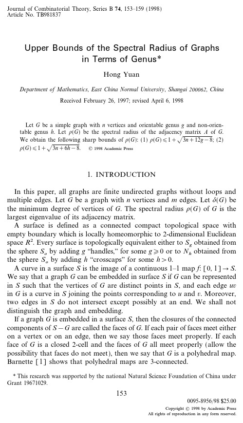
Let G be a simple graph with n vertices and orientable genus g and non-orien-
In 1978, A. J. Schwenk and R. J. Wilson [6] raised the question of what can be said about the eigenvalues of a planar graph. In 1988, the author [4] proved that the spectral radius of a planar graph with n vertices is less than - 5n&11. In 1993, Cao and Vince [2] proved that the spectral radius
* This research was supported by the national Natural Science Foundation of China under Grant 19671029.
153
0095-8956Â98 25.00
Copyright 1998 by Academic Press All rights of reproduction in any form reserved.
Lemma 1. Let G be a triangulation with n 4 vertices; then
离散数学双语专业词汇表

《离散数学》双语专业词汇表set:集合subset:子集element, member:成员,元素well-defined:良定,完全确定brace:花括号representation:表示sensible:有意义的rational number:有理数empty set:空集Venn diagram:文氏图contain(in):包含(于)universal set:全集finite (infinite) set:有限(无限)集cardinality:基数,势power set:幂集operation on sets:集合运算disjoint sets:不相交集intersection:交union:并complement of B with respect to A:A与B的差集symmetric difference:对称差commutative:可交换的associative:可结合的distributive:可分配的idempotent:等幂的de Morgan’s laws:德摩根律inclusion-exclusion principle:容斥原理sequence:序列subscript:下标recursive:递归explicit:显式的string:串,字符串set corresponding to a sequence:对应于序列的集合linear array(list):线性表characteristic function:特征函数countable(uncountable):可数(不可数)alphabet:字母表word:词empty sequence(string):空串catenation:合并,拼接regular expression:正则表达式division:除法multiple:倍数prime:素(数)algorithm:算法common divisor:公因子GCD(greatest common divisor):最大公因子LCM(least common multiple):最小公倍数Euclidian algorithm:欧几里得算法,辗转相除法pseudocode:伪码(拟码)matrix:矩阵square matrix:方阵row:行column:列entry(element):元素diagonal matrix:对角阵Boolean matrix:布尔矩阵join:并meet:交Boolean product:布尔乘积mathematical structure(system):数学结构(系统)closed with respect to:对…是封闭的binary operation:二元运算unary operation:一元运算identity:么元,单位元inverse:逆元statement, proposition:命题logical connective:命题联结词compound statement:复合命题propositional variable:命题变元negation:否定(式)truth table:真值表conjunction:合取disjunction:析取quantifier:量词universal quantification:全称量词化propositional function:命题公式predicate:谓词existential quantification:存在量词化converse:逆命题conditional statement, implication:条件式,蕴涵式consequent, conclusion:结论,后件contrapositive:逆否命题hypothesis:假设,前提,前件biconditional, equivalence:双条件式,等价logically equivalent:(逻辑)等价的contingency:可满足式tautology:永真(重言)式contradiction, absurdity:永假(矛盾)式logically follow:是…的逻辑结论rules of reference:推理规则modus ponens:肯定律m odus tollens:否定律indirect method:间接证明法proof by contradiction:反证法counterexample;反例basic step:基础步principle of mathematical induction:(第一)数学归纳法induction step:归纳步strong induction:第二数学归纳法relation:关系digraph:有向图ordered pair:有序对,序偶product set, Caretesian set:叉积,笛partition, quotient set:划分,商集block, cell:划分块,单元domain:定义域range:值域R-relative set:R相关集vertex(vertices):结点,顶点edge:边in-degree:入度out-degree:出度path:通路,路径cycle:回路connectivity relation:连通性关系reachability relation:可达性关系composition:复合reflexive:自反的irreflexive:反自反的empty relation:空关系symmetric:对称的asymmetric:非对称的antisymmetric:反对称的graph:无向图undirected edge:无向边adjacent vertices:邻接结点connected:连通的transitive:传递的equivalent relation:等价关系congruent to:与…同余modulus:模equivalence class:等价类linked list:链表storage cell:存储单元pointer:指针complementary relation:补关系inverse:逆关系closure:闭包symmetric closure:对称闭包reflexive closure:自反闭包composition:关系的复合transitive closure:传递闭包Warshal’s algorithm:Warshall算法function, mapping, transformation:函数,映射,变换argument:自变量value, image:值,像,应变量labeled digraph:标记有向图identity function on A:A上的恒等函数everywhere defined:处处有定义的onto:到上函数,满射one to one:单射,一对一函数bijection, one-to-one correspondence:双射,一一对应invertible function:可逆函数floor function:下取整函数ceiling function:上取整函数Boolean function:布尔函数base 2 exponential function:以2为底的指数函数logarithm function to the base n:以n为底的对数hashing function:杂凑函数key:键growth of function:函数增长same order:同阶lower order:低阶running time:运行时间permutation:置换,排列cyclic permutation:循环置换,轮换transposition:对换odd(even) permutation:奇(偶)置换order relation:序关系partial order:偏序关系partially ordered set, poset:偏序集dual:对偶comparable:可比较的linear order(total order):线序,全序linearly ordered set, chain:线(全)序集,链product partial order:积偏序lexicographic order:字典序Hasse diagram:哈斯图topological sorting:拓扑排序isomorphism:同构maximal(minimal) element:极大(小)元extremal element:极值元素greatest(least) element:最大(小)元unit element:么(单位)元zero element:零元upper(lower) bound:上(下)界least upper(greatest lower) bound:上(下)确界lattice:格join:,保联,并meet:保交,交sublattice:子格absorption property:吸收律bounded lattice:有界格distributive lattice:分配格complement:补元modular lattice:模格Boolean algebra:布尔代数involution property:对合律Boolean polynomial, Boolean expression:布尔多项式(表达式)or(and, not) gate:或(与,非)门inverter:反向器circuit design:线路设计minterm:极小项Karnaugh map:卡诺图tree:树root:根,根结点rooted tree:(有)根树level:层,parent:父结点offspring:子女结点siblings:兄弟结点height:树高leaf(leave):叶结点ordered tree:有序树n-tree:n-元树complete n-tree:完全n-元树(complete) binary tree:(完全)二元(叉)树descendant:后代subtree:子树positional tree:位置树positional binary tree:位置二元(叉)树doubly linked list:双向链表tree searching:树的搜索(遍历)traverse:遍历,周游preorder search:前序遍历Polish form:(表达式的)波兰表示inorder search:中序遍历postorder search:后序遍历reverse Polish form:(表达式的)逆波兰表示linked-list representation:链表表示undirected tree:无向树undirected edge:无向边adjacent vertices:邻接结点simple path:简单路径(通路)simple cycle:简单回路acyclic:无(简单)回路的spanning tree:生成树,支撑树Prim’s algorithm:Prim算法minimal spanning tree:最小生成树weighted graph:(赋)权图weight:树distance:距离nearest neighbor:最邻近结点greedy algorithm:贪婪算法optimal solution:最佳方法Kruskal’s algorithm:Kruskal算法graph:(无向)图vertex(vertices):结点edge:边end point:端点relationship:关系connection:连接degree of a vertex:结点的度loop:自回路path:路径isolated vertex:孤立结点adjacent vertices:邻接结点circuit:回路simple path(circuit):基本路径(回路) connected:连通的disconnected:不连通的component:分图discrete graph(null graph):零图complete graph:完全图regular graph:正规图,正则图linear graph:线性图subgraph:子图Euler path(circuit):欧拉路径(回路) Konisberg Bridge problem:哥尼斯堡七桥问题ordinance:法规recycle:回收,再循环bridge:桥,割边Hamiltonian path(circuit):哈密尔顿路径(回路)dodecahedron:正十二面体weight:权TSP(traveling salesperson problem):货郎担问题transport network:运输网络capacity:容量maximum flow:最大流source:源sink:汇conversation of flow:流的守恒value of a flow:流的值excess capacity:增值容量cut:割the capacity of a cut:割的容量matching problems:匹配问题matching function:匹配函数compatible with:与…相容maximal match:最大匹配complete match:完全匹配coloring graphs:图的着色proper coloring:正规着色chromatic number of G:G的色数map-coloring problem:地图着色问题conjecture:猜想planar graph:(可)平面图bland meats:未加调料的肉chromatic polynomial:着色多项式binary operation on a set A:集合A上的二元运算closed under the operation:运算对…是封闭的commutative:可交换的associative:可结合的idempotent:幂等的distributive:可分配的semigroup:半群product:积free semigroup generated by A:由A生成的自由半群identity(element):么(单位)元monoid:含么半群,独异点subsemigroup:子半群submonoid:子含么半群isomorphism:同构homomorphism:同态homomorphic image:同态像Kernel:同态核congruence relation:同余关系natural homomorphism:自然同态group:群inverse:逆元quotient group:商群Abelian group:交换(阿贝尔)群cancellation property:消去律multiplication table:运算表finite group:有限(阶)群order of a group:群的阶symmetric group:对称群subgroup:子群alternating group:交替群Klein 4 group:Klein四元群coset:陪集(left) right coset:(左)右陪集normal subgroup:正规(不变)子群prerequisite:预备知识virtually:几乎informal brand:不严格的那种notation:标记sensible:有意义的logician:逻辑学家extensively:广泛地,全面地commuter:经常往来于两地的人by convention:按常规,按惯例dimension:维(数) compatible:相容的discipline:学科reasoning:推理declarative sentence:陈述句n-tuple:n-元组component sentence:分句tacitly:默认generic element:任一元素algorithm verification:算法证明counting:计数factorial:阶乘combination:组合pigeonhole principle:鸽巢原理existence proof:存在性证明constructive proof:构造性证明category:类别,分类factor:因子consecutively:相继地probability(theory):概率(论) die:骰子probabilistic:概率性的sample space:样本空间event:事件certain event:必然事件impossible event:不可能事件mutually exclusive:互斥的,不相交的likelihood:可能性frequency of occurrence:出现次数(频率) summarize:总结,概括plausible:似乎可能的equally likely:等可能的,等概率的random selection(choose an object at random):随机选择terminology:术语expected value:期望值backtracking:回溯characteristic equation:特征方程linear homogeneous relation of degree k:k阶线性齐次关系binary relation:二元关系prescribe:命令,规定coordinate:坐标criteria:标准,准则gender:性别graduate school:研究生院generalize:推广notion:概念intuitively:直觉地verbally:用言语approach:方法,方式conversely:相反地pictorially:以图形方式restriction:限制direct flight:直飞航班tedious:冗长乏味的main diagonal:主对角线remainder:余数random access:随机访问sequential access:顺序访问custom:惯例polynomial:多项式substitution:替换multi-valued function:多值函数collision:冲突analysis of algorithm:算法分析sophisticated:复杂的set inclusion(containment):集合包含distinguish:区分analogous:类似的ordered triple:有序三元组recreational area:游乐场所multigraph:多重图pumping station:抽水站depot:货站,仓库relay station:转送站。
Quantum Monte Carlo

Contributed Talks (alphabetically ordered following the speaker’s surname)Hansj¨o rg AlbrecherReinhold KainhoferRobert F.TichyDepartment of MathematicsGraz University of TechnologySteyrergasse30/IIA-8010Graz,Austriae-mail:albrecher@tugraz.athttp://www.cis.TUGraz.at/mathaTitleSimulation Methods in Ruin Modelswith Non-linear Dividend Barriers1AbstractIn this paper we consider a collective risk reserve process of an insurance portfolio char-acterized by a homogeneous Poisson claim number process,a constant premiumflow and independent and identically distributed claims.In the presence of a non-linear dividend bar-rier strategy and interest on the free reserve we derive equations for the probability of ruin and the expected present value of dividend payments which give rise to several numerical number-theoretic solution techniques.For various claim size distributions and a parabolic barrier numerical tests and comparisons of these techniques are performed.In particular,the efficiency gain obtained by implementing low-discrepancy sequences instead of pseudorandom sequences is investigated.1Research supported by the Austrian Science Foundation Project S-8308MATJames B.AndersonDepartment of ChemistryPennsylvania State UniversityUniversity Park,Pennsylvania16802e-mail:jba@TitleQuantum Monte Carlo:Direct Calculation of Corrections to Trial Wave Functions and Their EnergiesAbstractWe will discuss an improved Monte Carlo method for calculating the differenceδbetweena true wavefunctionΨand an analytic trial wavefunctionΨ0.The method also producesa correction to the expectation value of the energy for the trial function.Applications to several sample problems as well as to the water molecule will be described.We have described previously a quantum Monte Carlo(QMC)method for the direct cal-culation of corrections to trial wavefunctions[1-3].Our improved method is much simplerto use.Like its predecessors the improved method gives(forfixed nodes)the differenceδbetween a true wavefunctionΨand a trial wavefunctionΨ0,but it gives in addition thedifference between the true energy E and the expectation value of the energy E var for the trial wavefunction.The statistical or sampling errors associated with the Monte Carlo procedures as well as any systematic errors occur only in the corrections.Thus,very accurate wavefunctions and energies may be corrected with very simple calculations.For systems with nodes the nodes are unchanged.The wavefunctions and energies for these systems are corrected to thefixed-node values-those corresponding to the exact solutionsfor thefixed nodes of the trial wavefunctions.The method has the very desirable features of:good wavefunction in/better wavefunction out...good energy in/better energy out.The ground state of the helium atom provides a simple example.We used as a trial wavefunc-tion the189-term Hylleraas function described by Schwartz[4]which is accurate to about10 digits.The true energy is known to at least13digits from the analytic variational calculationof Freund,Huxtable,and Morgan[5]with a more complex trial function.The expectation value for the trial function is−2.903724376180(0)hartrees.The calculated correction is−0.000000000856(2)hartrees which gives a corrected value of−2.903724377036(2) hartrees.This may be compared with the known value of−2.903724377034(0)hartrees.The water molecule presents the problem of nodes in the wavefunction as well as a much higher dimensionality.In this case the nodes arefixed in position by the use offixed-node QMC procedures[6]and the resulting energy obtained is thefixed-node energy for the nodesof the trial wavefunction.As in anyfixed-node calculation the energy obtained is a variationalupper bound to the true energy,and if the nodes are wrong the energy will be higher than the true energy.The trial function for this case was a simple SCF function,consisting of a single10x10 determinant of LCAO-MO terms of Slater-type orbitals without any Jastrow or other explicit electron correlation terms.The expectation value of the energy for the trial function and the fixed-node QMC energy were determined independently by standard methods.In this case the initial energy is−75.560hartrees,the calculated correction is−0.599hartrees, and the corrected value is−76.169(10)hartrees.This may be compared with the indepen-dently calculated value of−76.170(10)hartrees.Earlierfixed-node QMC calculations for systems of ten or more electrons have used single-determinant trial wavefunctions with Jastrow terms.With the improved correction procedure the need for accurate expectation values for the trial function requires eliminating the Jastrow terms,but it may make practical the use of many more determinants in the trial function. This is likely to give improved node locations and lead to much lower node location errors. The sign problem of quantum Monte Carlo for large systems would not be eliminated but it might be significantly reduced.[1]J.B.Anderson and B.H.Freihaut,put.Phys.31,425(1979).[2]J.B.Anderson,J.Chem.Phys.73,3897(1980).[3]J.B.Anderson,M.Mella,and A.Luechow,in Recent Advances in Quantum Monte Carlo Methods,(W.A.Lester,Jr.,Ed.,World Scientific,Singapore)1997,pp.21-38.[4]C.Schwartz,Phys.Rev.128,1146(1962).[5]D.E.Freund,B.D.Huxtable,and J.D.Morgan III,Phys.Rev.A29,980(1984).[6]J.B.Anderson,J.Chem.Phys.63,1499(1975).James B.Anderson1Lyle N.Long21Department of Chemistry2Department of Aerospace EngineeringPennsylvania State UniversityUniversity Park,Pennsylvania16802e-mail:jba@TitleThe Simulation of DetonationsAbstractThe Direct Simulation Monte Carlo(DSMC)method(1,2)has been found remarkably suc-cessful for predicting and understanding a number of difficult problems in rarefied gas dynam-ics.Extension to chemical reaction systems has provided a very powerful tool for reacting gas mixtures with non-Maxwellian velocity distributions,with non-Boltzmann state distribu-tions,with coupled gas-dynamic and reaction effects,with concentration gradients,and with many other effects difficult or impossible to treat in any other way.Examples of systems which may be treated includeflames and explosions,shock waves and detonations,reactions and energy transfer in laser cavities,upper atmosphere reactions,and many,many others.In this paper we will discuss the application of the DSMC method to the problem of detonations, a classic and extreme example of the coupling of gas dynamics and chemical kinetics. Although a Monte Carlo simulation of a gas was described by Lord Kelvin in1901(3),it was not until the1960’s that the use of such simulations became practical for solving problems in thefield of rarefied gas dynamics.The combination of an efficient sampling method by Bird(1)in1963with high speed computers made possible the nearly exact simulation of a number of systems that had earlier been impossible to analyze.The current generation of computers makes it possible to consider much more ambitious applications:those in which chemical reactions are important.A detonation wave travels at supersonic speed in a reactive gas mixture and is driven by the energy released in exothermic reaction within the wave.The modern theory of detonations begins with the work of Chapman and of Jouguet about1900,and their work has been extended by a number of others,in particular by Zeldovich(4),von Neumann(5),and D¨o ring(6).These three arrived independently at an expression,the ZVD expression,giving the velocity of a detonation wave as the velocity of sound in the completely burned gases when the shock wave precedes the reaction.In order to simplify our DSMC calculations and to clarify the results by eliminating extrane-ous effects,we considered the special case of the reaction of A+M→B+M in which the masses of A,B,and M are equal.The gases were specified as ideal and calorically perfect with constant heat capacities.The cross-sections for reaction were specified as simple functions of collision energy corresponding to Arrhenius behavior.Calculations were carried out for a variety of conditions-covering a wide range of exothermicities and reaction rate parameters.The simulations provide complete details of the properties of the system as they vary across the detonation wave.A variety of interesting results have been obtained.Temperature, density,and reaction-rate peaks may be separated.Temperature and density maxima depend strongly on reaction rate.The thickness of the reaction zone depends strongly on conditions. The results provide severe tests for some of the earlier theoretical models of detonations.(1)G.A.Bird,Phys.Fluids6,1518(1963).(2)G.A.Bird,Molecular Gas Dynamics and the Direct Simulation of Gasflows,Clarendon Press,Oxford,1994.(3)Lord Kelvin,Phil.Mag.(London)2,1(1901).(4)Y.B.Zeldovich,J.Exptl.Theoret.Phys.(U.S.S.R.)10,542(1940).(5)J.von Neumann,O.S.R.D.Rept.No.549(1942).(6)W.D¨o ring,Ann.Physik43,421(1943).James B.AndersonDepartment of ChemistryPennsylvania State UniversityUniversity Park,Pennsylvania16802e-mail:jba@TitleMonte Carlo Treatment of UV Light Imprisonment in Fluorescent LampsAbstractThe efficiency of a modernfluorescent lamp is reduced significantly by self-absorption of the2537-˚A ultraviolet radiation emitted from mercury within the lamp(1).Experimental measurements indicate the efficiency may be increased by tailoring the isotopic composition of the mercury as by the addition of19680Hg to natural mercury(2).Radiation emitted by an atom in an optical transition from an excited state to the ground state is commonly called”resonance radiation.”Since the cross-section for absorption of this radiation by atoms in the ground state is typically large,a quantum of radiation released within a chamber containing emitting atoms is likely to be reabsorbed before reaching the walls of the chamber.The absorbing atom may subsequently emit the radiation,and the emission-absorption steps may be repeated a large number of times.The radiation is described as”imprisoned”or”trapped”when the number of steps required for escape to the walls is large.The imprisonment of resonance radiation in the electrical discharge offluorescent lamps can be treated by Monte Carlo methods.The calculation of radiation and energy transfer is essentially a simulation of the processes occurring within the lamp.Following the initial excitation of a mercury atom its energy(or photon)is tracked from atom to atom until the photon either leaves the system or is lost by quenching in the collision of an excited atom with another atom.The procedure is repeated thousands of times to obtain a reliable estimate of the overall exit probability and a spectrum of the exit radiation with an acceptable noise level.Many of the variables required in the calculation are selected from appropriately weighted distributions.For example,an initial isotopic species to be excited is selected with a prob-ability proportional to its fraction in the mixture.The direction of an emitted photon is selected at random in three dimensions.The frequency of the emitted radiation is selected from a Voigt distribution with the line center corresponding to that of the excited atom.The free path of a photon is selected from the calculated distribution of free paths for a photon with the same wavelength.The effects of emission and absorption linewidths,hyperfine splitting,isotopic composition, collisional transfers of excitation,and quenching are explicitly included in the calculations. The calculated spectra of the emitted radiation are in good agreement with measured spectra for several combinations of lamp temperature and mercury composition.The complete detailsof the hyperfine structure of the spectra including multiple peaks for the isotopes and line-reversal are accurately reproduced.Also in agreement with experiments,the addition of 196Hg to natural mercury is found to increase lamp efficiency.80(1)J.F.Waymouth,”Physics for Fun and Profit”,Physics Today54,38(2001).(2)J.Maya,M.W.Grossman,guschenko,and J.F.Waymouth,Science226,435 (1984).F.M.Bufler1A.SchenkW.FichtnerInstitut f¨u r Integrierte SystemeETH Z¨u richGloriastrasse35CH-8092Z¨u rich,Switzerlande-mail:bufler@iis.ee.ethz.chhttp://www.iis.ee.ethz.ch/portrait/staff/bufler.en.htmlTitleProof of a Simple Time–Step Propagation Schemefor Monte Carlo Simulation2AbstractMonte Carlo simulation has been established as a stochastic method for the solution of the Boltzmann transport equation(BE)(1;2;3)which is an integro–differential equation for the electron distribution function.Its solution can be used to compute macroscopic quantities such as the electron density or the current density.Since the BE considers the electron drift in the electricfield as well as the scattering events at a microscopic level,it allows one to take physical effects occurring in deep submicron metal–oxide–semiconductorfield–effect transistors(MOSFETs)into account,for example ballistic and hot–electron transport. Various algorithms have been developed to improve the computational efficiency of the Monte Carlo simulation.Among them is the self–scattering scheme of Rees(4)which uses an upper estimateΓof the scattering rate to greatly facilitate the determination of the collisionless flight–time.In order to avoid at the same time a large number of self–scattering events involved with a global upper estimation,a variableΓscheme is often being employed(1;5; 6;7).This scheme is especially useful for full–band Monte Carlo(FBMC)simulation where the electronic band structure is not described by an analytical formula,but computed by the empirical pseudopotential method and stored in a table.Here it is natural to assign a differentΓto each element of the discretized phase–space.However,for large selected free–flight times the electron will leave the original phase–space element and theflight–time is usually adjusted in a rather complicated manner in order to accomodate the change of Γ(5;6;7).It is the aim of this paper to show that such an adjustment is not necessary, but that simply a newflight–time can be stochastically selected if the border of the original phase–space element is crossed.The proof is based on the calculation of the probability that there is no scattering between the times0and t.This event is equivalent to the time of thefirst scattering,t s,being larger than t and therefore the event will be denoted by{t s∈(0,t)}.When the time interval(0,t) is decomposed into two not necessarily equidistant time intervals,the above event can be represented as the intersection of the events that there is no scattering in any of the two intervals,i.e.we have for the corresponding probability1Speaker2Research supported by the Kommission f¨u r Technologie und Innovation(KTI),project4082.2P ({t s ∈(0,t )})=P ({t s ∈(0,t 1)}∩{t s ∈(t 1,t )})(1)Equation (1)is completely general and does not refer to the Boltzmann transport equation (BE).On the other hand,in the specific case of the BE,this probability is given by (8;9)P BE ({t s ∈(0,t )})=exp − t 0S (k (τ))dτ(2)where S is the scattering rate and k (τ)the electron’s momentum at time τ.The exponential in Eq.(2)allows a factorization according toP BE ({t s ∈(0,t )})=P BE ({t s ∈(0,t 1)}∩{t s ∈(t 1,t )})=exp − t 10S (k (τ))dτ+ tt 1S (k (τ))dτ=exp(−t 10S (k (τ))dτ)×exp(− t t 1S (k (τ))dτ)=P BE ({t s ∈(0,t 1)})×P BE ({t s ∈(t 1,t )}).(3)Since P (A ∩B )=P (A )×P (B )for stochastically independent events A and B ,Eq.(3)proves that the absence of scattering in the interval (t 1,t )is independent of the absence of scattering in the interval (0,t 1).In other words,when the event that the first scattering does not occur before t 1is realized (with the help of a random number r evenly distributed in [0,1)),the particle can be propagated until t 1and then a new random number can be generated to decide whether scattering occurs in the next interval.For an explicit treatment of the opposite event,we observe regardless of the above consider-ations that Eq.(2)shows for t →∞that there will occur,at some time,the first scattering.It follows that P BE ({t s ∈(0,t 1)})=1−P BE ({t s ∈(0,t 1)})=1−exp(− t 1S (k (τ))dτ).(4)Hence,in the self–scattering scheme with an upper estimation Γof S (k ),the event of the first scattering occurring before t 1is realized for r <1−exp(−Γt 1).In this case the particle ispropagated as usual until t s =−1Γln(1−r ).In fact,the above inequality leads to −ln(1−r )<Γt 1and therefore to t s <t 1.In summary,the above considerations have proven the following propagation scheme.First,a random number is used to determine whether the first scattering occurs before a given time t 1.In this case,the particle is propagated according to the corresponding free–flight time,otherwise until t 1.Then a new,possibly different time step is defined and the procedure is repeated.The validity of this scheme has been verified by an explicit comparison with the standard Monte Carlo scheme and was used for an efficient FBMC device simulation (10).References[1]C.Jacoboni and P.Lugli,The Monte Carlo Method for Semiconductor Device Simulation(Springer,Wien,1989).[2]Monte Carlo Device Simulation:Full Band and Beyond,edited by K.Hess(Kluwer,Boston,1991).[3]M.V.Fischetti and ux,Phys.Rev.B38,9721(1988).[4]H.D.Rees,Phys.Lett.A26,416(1968).[5]J.Bude and R.K.Smith,Semicond.Sci.Technol.9,840(1994).[6]E.Sangiorgi,B.Ricco,and F.Venturi,IEEE puter–Aided Des.7,259(1988).[7]C.Jungemann,S.Keith,M.Bartels,and B.Meinerzhagen,IEICE Trans.Electron.E82–C,870(1999).[8]W.Fawcett,A.D.Boardman,and S.Swain,J.Phys.Chem.Solids31,1963(1970).[9]A.Reklaitis,Phys.Lett.A88,367(1982).[10]F.M.Bufler,A.Schenk,and W.Fichtner,IEEE Trans.Electron Devices47,1891(2000).Ervin Dubaric12Urban EnglundMats Hjelm2Hans-Erik NilssonDepartment of Information Technology and MediaMid-Sweden UniversitySE-85170Sundsvall,SwedenTitleMonte Carlo Simulation of the Transient Response ofSingle Photon Absorption in X-ray Pixel DetectorsAbstractA Monte Carlo method to simulate the transient response of X-ray pixel detectors is proposed. The method combines the use of a state of the art photon transport and absorption model with full band Monte Carlo simulation of the semiconductor detector.The method has been used to study the transient response of a single photon absorption event in three different X-ray pixel detectors,one photon counting detector,one integrating detector and one scintillator coated integrating pixel detector.In a photon counting detector each absorbed photon is detected as a current pulse,which in turn triggers a digital counter.In an integrating version, the current is integrated by a charge sensitive amplifier,producing an analog signal as the detector output.Coating an integrating detector with a scintillating layer increases the number of photons that can be detected by the detector.In this case the signal is generated both by X-ray photons captured in the scintillator and by X-ray photons captured directly in the semiconductor.There are different reasons to study the single photon absorption in these detector structures.In the photon counting configuration the actual output signal is the transient response of a single photon absorption event.On the other hand,in the integrating configuration the single photon event may be used to study charge sharing effects introduced by absorption in the boundary region of the pixel detector.In this case the interest is primarily to track the generated carriers as they are distributed among the neighboring pixels.Introduction to X-ray imaging detectorsAn X-ray detector can either be made from a heavy semiconductor with high stopping power for X-rays or a scintillator can be used to convert the X-ray photons to visible light,which is then sensed by a pixel sensor.In a single layer detector,made from a heavy semiconductor, the response of the system is only determined by the properties of the semiconductor.In a detector system where a scintillator and photo-detector form a two-layer system the response of the system depends both on the properties of the scintillator and the properties of the photo-detector.1Speaker;e-mail:Ervin.Dubaric@ite.mh.se2also:Solid State Electronics,Department of Microelectronics and Information Technology,Royal Institute of Technology(KTH),Electrum229,SE-16440Kista,SwedenIn a scintillator coated X-ray imaging sensor the signal is generated both by X-ray photons captured in the scintillator and by X-ray photons captured in the semiconductor sensor.Since the amount of generated charge in the semiconductor,per MeV of absorbed X-ray energy, differs significantly depending on where the absorption occurred,the image properties are affected both by the scintillator and the semiconductor sensor.In a photon counting system a pure semiconductor detector is used.The detector should have high charge collection efficiency,which demands the use of a very pure semiconductor material in order to obtained the highest possibleµ·τproduct.A typical sensor consists of a shallow PN junction,with as large depletion region in the bulk as possible.SimulationA method to simulate these types of detectors is proposed.The method is based on the use of two different Monte Carlo simulation software packages.The photon transport is simulated using the commercially available MCNP software and the charge carrier transport is simulated using our own full band Monte Carlo device simulator.A third,in house software,is used as a link between the two Monte Carlo simulators when simulating the scintillator coated detector.This in house software calculates the distribution and absorption of visible light in the semiconductor resulting from an X-ray absorption in the scintillating layer.A large part of this light is absorbed near the surface of the nearest pixel detector.However,depending on the design of the scintillating layer charge sharing may occur as the light is scattered towards neighboring pixels.The simulation procedure starts by simulating the detector structure in MCNP.MCNP cal-culates the trajectory of incoming X-ray photons using a Monte Carlo approach.The tra-jectories of the simulated photons are investigated and a number of particularly interesting trajectories is selected.Each of these trajectories(including data for deposited charge along the path)is used as input in the full band Monte Carlo device simulator.In the case of an absorption in the scintillator layer,the in house light scattering program is used to transfer the signal down to the semiconductor detector.The response of the detector is then simulated using the full band Monte Carlo device simulator.There are several important issues that need to be addressed in simulation of the detector re-sponse.The detector structures are usually very large which makes self-consistent simulation very time consuming.In this work we have used self-consistent simulations in the photon counting detector where the absorption event occurs in the depletion region.In this way we may directly record the current pulse at the detector electrodes.In the case of the integrating detectors we are following the carriers as they move towards collection.The charge sharing is studied by comparing the number of carriers absorbed at different pixel locations.The actual current pulse is not recorded,which allows us to use a constant potential profile during the simulation.The potential profile has been obtained from drift-diffusion simulation of a dark detector.Simulation result of different detector structures is presented using this new approach.The result has primarily been used to visualize the charge sharing in pixel arrays and to study the transient response as a function of position of the absorption in photon counting detectors.Lucian ShifrenDavid K.Ferry1Department of Electrical EngineeringCenter for Solid State Electronics ResearchArizona State UniversityTempe,Arizona,85287-5706,USAe-mail:ferry@/~nanoTitleA Particle Monte Carlo SimulationBased on the Wigner Function DistributionAbstractWe present results of a new particle-based ensemble Monte Carlo(EMC)simulation of the Wigner distribution function(WDF).EMC of quantum systems is difficult to implement due to the particle nature of the method and the wave-like nature of the quantum phenomena. We introduced a new property for the particles,which we call the particle affinity,which allows the overall distribution to assume negative and partial electron values.We divide the simulation into two system,thefirst being the EMC regime,and the second being the WDF regime.Although two systems exists,the two systems work simultaneously within the simulation.Within the EMC regime,all particles in the system are treated equally,that is,all particles have an assigned position and momentum,all particles drift and are accelerated and scattered.In the WDF regime however,along with the pre-mentioned properties assigned to the electrons,we also assign the electrons an affinity.The affinity value the electron may take must have a magnitude less then one,where a value of one corresponds to a“present”electron,a value of minus one corresponds to a“minus presence,”and any value in between accounts for the partial“presence”or“minus presence”of an electron.Within the simulation, all particles drift and are accelerated,independent of what their affinities might be.However, when calculating the Wigner potential(which is a non-local potential),we switch to the WDF regime.Here,the Wigner distribution is defined byf(x,k)=δ(x−x i)δ(k−k i)A(i),(1)iwhere the delta functions represent the presence of a particle from the EMC regime,and A,the affinity,represents the value of the electron which is contributed to the distribution. Results using this method are shown in Fig1.The results show a gaussian wave packet which has tunneled through a potential barrier.This result has been compared to two fully quantum mechanical simulations,namely,a full solution of Schr¨o dinger equations and the direct solution of the WDF.The transmission coefficients of all three cases is∼0.35,which corresponds to the analytical value determined from simple tunneling theory.The new EMC 1Speaker;Research supported by the Office of Naval Researchmethod has also been checked against the other methods using Bohm trajectories which show remarkable similarity to each other.The EMC method correctly shows that the Bohm trajectories originating from the front of the gaussian packet are the ones that tunnel.Not only does the particle solution calculate the correct transmission and give the correct Bohm trajectories,but also,the resulting density displays interference effects and correlations,seen in Fig1,that have previously only been seen in fully quantum mechanical simulations.Cor-relations are fully quantum mechanical and allow for time reversal in quantum systems.We believe this to be thefirst particle-based simulation that correctly accounts for interference, correlation and tunneling.Figure1:Distribution function from EMC solution of a gaussian which has tunneled through a potential barrier2nm wide and0.3eV high.S.M.RameyD.K.Ferry1Department of Electrical Engineering andCenter for Solid State Electronics ResearchArizona State UniversityTempe,Arizona,85287-5706USAe-mail:ferry@/~nanoTitleMonte Carlo Modeling of Quantum Effects inSemiconductor Devices with Effective PotentialsAbstractAs modern devices continue to scale to smaller sizes,it has become imperative to include quantum mechanical effects when modeling device behavior.We have recently proposed the use of the effective potential to treat the quantum mechanical effects of confinement in the region adjacent to the oxide interface[1].In this work,we illustrate the use of the effective potential as a fast and simple method of including these effects in Monte Carlo simulation of ultrasmall SOI MOSFETs.The effective potential concept uses the fact that as the electron moves,the edge of the wave packet encounters variations in the potential profile before the center of the wave packet. Mathematically,this effect at a point(x i,y j)can be treated as the convolution of the potential with the Gaussian wave packet as follows:V eff(x i,y j)=V(x,y)G(x,y;x i,y i;a x,a y)dxdywhere G is the Gaussian function with standard deviations a x and a y.The spread of the wave packet is determined by the thermal de Broglie wavelength for the lateral direction and the confining potential in the transverse direction[2,3].The effective potential is included in the Monte Carlo transport simulation by applying the above convolution to the potential found from solution of the Poisson equation.As an example,the resulting effective potential profile for an SOI NMOSFET with a30nm silicon layer is illustrated in Fig.1for an applied gate and drain voltage of1.2volts.The potential clearly increases at the oxide interfaces as a result of the convolution with the electron wave packet.As a result of this potential increase,the electrons experience a strong electricfield, which is then included in the Monte Carlo transport kernel.As a demonstration of this,Fig.2shows the electron density distribution that corresponds to the potential profile in Fig.1.The average electron density set-back from the gate interface is about2.5nm,which is consistent with results shown elsewhere[3].1Speaker;Research supported by the Semiconductor Research Corporation。
2011AMC10美国数学竞赛A卷附中文翻译和答案

2011AMC10美国数学竞赛A卷1. A cell phone plan costs $20 each month, plus 5¢ per text message sent, plus 10¢ for each minute used over 30 hours. In January Michelle sent 100 text messages and talked for 30.5 hours. How much did she have to pay?(A) $24.00 (B) $24.50 (C) $25.50 (D) $28.00 (E) $30.002. A small bottle of shampoo can hold 35 milliliters of shampoo, Whereas a large bottle can hold 500 milliliters of shampoo. Jasmine wants to buy the minimum number of small bottles necessary to completely fill a large bottle. How many bottles must she buy?(A) 11 (B) 12 (C) 13 (D) 14 (E) 153. Suppose [a b] denotes the average of a and b, and {a b c} denotes the average of a, b, and c. What is {{1 1 0} [0 1] 0}?(A) 29(B)518(C)13(D) 718(E) 234. Let X and Y be the following sums of arithmetic sequences: X= 10 + 12 + 14 + …+ 100.Y= 12 + 14 + 16 + …+ 102.What is the value of Y X?(A) 92 (B) 98 (C) 100 (D) 102 (E) 1125. At an elementary school, the students in third grade, fourth grade, and fifth grade run an average of 12, 15, and 10 minutes per day, respectively. There are twice as many third graders as fourth graders, and twice as many fourth graders as fifth graders. What is the average number of minutes run per day by these students?(A) 12 (B) 373 (C) 887 (D) 13 (E) 146. Set A has 20 elements, and set B has 15 elements. What is the smallest possible number of elements in A ∪B, the union of A and B?(A) 5(B) 15 (C) 20 (D) 35 (E) 3007. Which of the following equations does NOT have a solution?(A)2(7)0x +=(B) -350x += (C) 20= (D)80= (E) -340x -=8. Last summer 30% of the birds living on Town Lake were geese, 25% were swans, 10% were herons, and 35% were ducks. What percent of the birds that were not swans were geese?(A) 20(B) 30 (C) 40 (D) 50 (E) 609. A rectangular region is bounded by the graphs of the equations y=a, y=-b, x=-c, and x=d, where a, b, c, and d are all positive numbers. Which of the following represents the area of this region?(A) ac + ad + bc + bd (B) ac – ad + bc – bd (C) ac + ad – bc – bd(D) –ac –ad + bc + bd (E) ac – ad – bc + bd10. A majority of the 20 students in Ms. Deameanor’s class bought pencils at the school bookstore. Each of these students bought the same number of pencils, and this number was greater than 1. The cost of a pencil in cents was greater than the number of pencils each student bought, and the total cost of all the pencils was $17.71. What was the cost of a pencil in cents?(A) 7(B) 11 (C) 17 (D) 23 (E) 7711. Square EFGH has one vertex on each side of square ABCD. Point E is on AB with AE=7·EB. What is the ratio of the area of EFGH to the area of ABCD?(A)4964 (B) 2532 (C) 78 (D) (E)12. The players on a basketball team made some three-point shots, some two-point shots, some one-point free throws. They scored as many points with two-point shots as with three-point shots. Their number of successful free throws was one more than their number of successful two-point shots. The team’s total score was 61 points. How many free throws did they make?(A) 13(B) 14 (C) 15 (D) 16 (E) 1713. How many even integers are there between 200 and 700 whose digits are alldifferent and come from the set {1, 2, 5, 7, 8, 9}?(A) 12(B) 20 (C) 72 (D) 120 (E) 20014. A pair of standard 6-sided fair dice is rolled once. The sum of the numbers rolled determines the diameter of a circle. What is the probability that the numerical value of the area of the circle is less than the numerical value of the circle’s circumference? (A)136 (B) 112 (C) 16 (D) 14 (E) 51815. Roy bought a new battery-gasoline hybrid car. On a trip the car ran exclusively on its battery for the first 40 miles, then ran exclusively on gasoline for the rest of the trip, using gasoline at a rate of 0.02 gallons per mile. On the whole trip he averaged 55 miles per gallon. How long was the trip in miles?(A) 140(B) 240 (C) 440 (D) 640 (E) 84016. Which of the following in equal to(A)(B) (C) 2 (D) (E) 617. In the eight-term sequence A, B, C, D, E, F, G , H, the value of C is 5 and the sum of any three consecutive terms is 30. What is A + H?(A) 17(B) 18 (C) 25 (D) 26 (E) 4318. Circles A, B, and C each have radius 1. Circles A and B share one point oftangency. Circle C has a point of tangency with the midpoint of AB. What is the area inside Circle C but outside Circle A and Circle B? (A) 32π- (B) 2π (C) 2 (D) 34π (E) 12π+19. In 1991 the population of a town was a perfect square. Ten years later, after an increase of 150 people, the population was 9 more than a perfect square. Now, in 2011, with an increase of another 150 people, the population is once again a perfect square. Which of the following is closest to the percent growth of the town’s popu lation during this twenty-year period?(A) 42(B) 47 (C) 52 (D) 57 (E) 6220. Two points on the circumference of a circle of radius r are selected independently and at random. From each point a chord of length r is drawn in a clockwise direction. What is the probability that the two chords intersect? (A)16 (B) 15 (C) 14 (D) 13 (E) 1221. Two counterfeit coins of equal weight are mixed with 8 identical genuine coins. The weight of each of the counterfeit coins is different from the weight of each of the genuine coins. A pair of coins is selected at random without replacement from the 10 coins. A second pair is selected at random without replacement from the remaining 8 coins. The combined weight of the first pair is equal to the combined weight of the second pair. What is the probability that all 4 selected coins are genuine?(A) 711(B) 913(C) 1115(D) 1519(E) 151622. Each vertex of convex pentagon ABCDE is to be assigned a color. There are 6 colors to choose from, and the ends of each diagonal must have different colors. How many different colorings are possible?(A) 2500 (B) 2880 (C) 3120 (D) 3250 (E) 375023. Seven students count from 1 to 1000 as follows:·Alice says all the numbers, except she skips the middle number in each consecutive group of thre e numbers. That is Alice says 1, 3, 4, 6, 7, 9, …, 997, 999, 1000.·Barbara says all of the numbers that Alice doesn’t say, except she also skips the middle number in each consecutive grope of three numbers.·Candice says all of the numbers that neither Alice nor Barbara says, except she also skips the middle number in each consecutive group of three numbers. ·Debbie, Eliza, and Fatima say all of the numbers that none of the students with the first names beginning before theirs in the alphabet say, except each also skips the middle number in each of her consecutive groups of three numbers.·Finally, George says the only number that no one else says.What number does George say?(A) 37 (B) 242 (C) 365 (D) 728 (E) 99824. Two distinct regular tetrahedra have all their vertices among the vertices of thesame unit cube. What is the volume of the region formed by the intersection of the tetrahedra?(A)112 (B) (C) (D) 16 (E)25. Let R be a square region and 4n an integer. A point X in the interior of R is called n-ray partitional if there are n rays emanating from X that divide R into N triangles of equal area. How many points are 100-ray partitional but not 60-ray partitional?(A) 1500(B) 1560 (C) 2320 (D) 2480 (E) 25002011AMC10美国数学竞赛A 卷1. 某通讯公司手机每个月基本费为20美元, 每传送一则简讯收 5美分(一美元=100 美分)。
图论第五章
Ch.5. Coloring of Graphs
4
Graph Theory
Clique number
5.1.6
The clique number of a graph G, written ω(G), is the maximum size of a set of pairwise adjacent vertices (clique) in G.
Ch.5. Coloring of Graphs
11
Graph Theory
Proposition 5.1.16. If G is an interval graph, then (G) =ω(G)
Proof: Order the vertices according to the left endpoints of the intervals in an interval representation. Apply greedy coloring, and suppose that x receives k, the maximum color assigned. Since x does not receive a smaller color, the left endpoint a of its interval belongs also to intervals that already have colors 1 through k-1. These intervals all share the point a, so we have a k-clique consisting of x and neighbors of x with colors 1 through k-1. Hence ω(G) ≥ k ≥ (G). Since (G) ≥ ω(G) always, this coloring is optimal.
Granular material flows
Granular material flows –An overviewCharles S.Campbell ⁎Aerospace and Mechanical Engineering,University of Southern California,Los Angeles,CA 90089-1453,USAReceived 6June 2005;received in revised form 19August 2005AbstractThe paper attempts to give a critical overview of the field of granular flow with attention both to the history and the underlying physics that govern the field.It starts with a discussion of the basic transport mechanisms in a granular flow.It continues with a discussion of contact mechanics –the way that individual particles see each other mechanically.It then discusses the historical limiting regimes of granular flow,the Quasistatic and the Rapid-Flow regimes.Finally,it concludes with a review of the Elastic picture of granular flow,which both unifies the Quasistatic and Rapid regimes and fills in the intervening space.It shows that the rheological behavior of granular systems changes with system scale constraints,and,in particular,that the materials behave differently under controlled-stress and controlled-concentration conditions.The Elastic model defines an entire flowmap of granular flow and thus allows one to place boundaries on where the Quasistatic and Rapid-Flow models (sometimes called kinetic theory models)are something of a red herring and cannot be applied to common granular flows.©2005Elsevier B.V .All rights reserved.Keywords:Transport mechanism;Quasistatic regime;Rapid-Flow regime;Granular flow1.IntroductionUnder the correct conditions,a granular solid can flow like a fluid.This was probably first recorded be Lucretius (ca.98–55B.C.),who wrote “One can scoop up poppy seeds with a ladle as easily as if they were water and,when dipping the ladle,the seeds flow in a continuous stream,”(quotation taken from Jacques [1]).As long as there has been mining and agriculture,man has attempted to exploit the flowability of granular solids to ease handling and storage problems.In particular,the ability of gravity to drive a granular flow,as noted by Lucretius,greatly simplifies and provides a cost-free mechanism of transport.As a result,the most common granular handling devices,chutes and hoppers,are gravity-driven flows.Yet the design of granular systems is still something of a black art,in part because even the most basic flow mechanisms of granular materials are not well understood.In fact,science has not identified the set of material properties that control the flow behavior.For the purposes of this article,a granular solid is taken to be a collection of discrete solid particles.In general the spaces between the particles are filled with an interstitial fluid,usuallyair.However,it will be assumed herein that the particles are large and heavy in the sense that they are immune to effects of the interstitial fluid.For the most part we will also ignore cohesion between particles;cohesion arises from surface forces or related phenomena such as liquid bridges,both of which act on the surface area and thus can generally be neglected for large particles with small surface area to volume ratios.Note that these requirements collectively define what is meant by “large ”although those criteria cannot yet be quantitatively defined by a set of dimensionless parameters.This paper grew out of a long lecture given to the Ohio State summer course on Powder Technology.It is an attempt to put the state of knowledge of granular flows into perspective.It is not intended to be a review article,in the sense that I am not trying to mention every paper written on the subject,but instead attempt to hit the highpoints and give a critical and balanced view to the whole subject.2.Internal force transmissionThe unique features of granular material arise from the manner in which force is internally transmitted.In continuum mechanics this is represented by a stress tensor τ,each component of which τij represents the force in the i-directionPowder Technology 162(2006)208–229⁎Corresponding author.E-mail address:campbell@.0032-5910/$-see front matter ©2005Elsevier B.V .All rights reserved.doi:10.1016/j.powtec.2005.12.008on a surface with outward pointing normal unit vector in the j direction.There are two internal modes of stress transmission.The first or Contact Stress ,τc is due to force transmission across interparticle contacts.Thus a force F c applied at a contact can be thought of as being transmitted in the direction of the vector l that connects the centers of mass of the two particles involved.(The length of l is the distance between the particle centers.)When averaged 〈〉over time and volume,this yields the Contact stress tensor:t c ¼h F c l ið1Þ(If the forces are transmitted collisionally,this is sometimes called the Collisional Stress tensor).This is shown schemati-cally in Fig.1a.Note that F c need not point in the direction of l ;when coupled with the fact that the averaging volume must be larger than a particle (and not allowed to shrink to infinitesimal size as in standard continuum mechanics),this means that the contact stress tensor need not be symmetric.Any symmetry is balanced by gradients in a couple-stress tensor that governs the transmission of torques internal to the material (see [2]).If the particles are moving,there will be some degree of internal momentum transport due to the motion of an individual particle as it moves relative to the bulk material,carrying its momentum with it as illustrated in Fig.1b.If u ′represents the velocity of that relative motion,then one defines a Streaming Stress Tensor τs analogous to the Reynolds stress tensor in turbulent flow.t s ¼q p v h u V u V ið2ÞHere ρp is the density of the solid material and νis the “solid-fraction ”or solid concentration,the fraction of a unit volume occupied by the particles (so that ρp νis the bulk density of the solid phase).The streaming stresses will only be significant at small concentrations when contacts are infrequent and in cases where the random particle velocity u ′is large.Common granular flows,such as hoppers,chutes and landslides are densely packed with solid concentrations well above 50%by volume.It is possible to obtain flows at a small concentration,but they are limited to high-speed laboratory shear cells,computer simulations and perhaps the rings of Saturn.As such,the contact stresses will dominate and the streaming stresses can usually be neglected.3.Contact forcesIn a dense granular flow,forces are largely generated by interparticle contacts.The contact forces are how the particles “see ”one another mechanically.Imagine the two spherical particles shown in Fig.2.As long as linear elasticity applies,the normal force on the contact will proportional to EA ε,E is the Young's modulus,A is the contact area and εis the local strain.The strain,ε=δ/L where δis the depth of the contact deformation (the distance the contact has been compressed)and L is an appropriate length scale.For the contact between two spheres shown in Fig.2,note that the contact area A is the zero on the unloaded contact to the left and increases when the particles are pressed together as on the right.The fact that both the area A and the strain ε,change simultaneously as the particle is deformed,leads to non-linearity of the contact response.In 1882,Hertz [3]derived an elastic solution for the contact between bodies.The solution is not exact as often thought,but contains an implicit assumption that the square root of the contact area is small compared to both the local radius of curvature and the overall dimensions of the body.The normal force exerted on a contact between two bodies of local curvature R is:f n ¼43R 1=2E 1Àm2d 3=2ð3Þ(from Johnson [4]),where E is the Young's modulus,and υis Poisson's ratio.This corresponds to a normal stiffness:k ¼d f n d d¼2R 1=2E 1Àm d 1=2ð4ÞSubstituting for δfrom (2),one can write the stiffness in termsof f n .k ¼61=3R 1=3E1Àm2 2=3f 1=3n ð5ÞFig.1.The two mechanisms of internal momentum transport.(a)Contacttransport:Here momentum crosses the imaginary surface (the dashed line)as the result of the contact force F c which can be thought of as transporting momentum between the centers of the particles along the vector l .(b)Streaming transport:Here the momentum of the particles is carried across the imaginary surface due to the random motion of the particles in a manner analogous to the transport of momentum in the kinetic theory of dilutegases.Fig.2.A schematic of the contact between two spheres of radius R generated bythe application of a force F .Here A is the area of the contact and δis the deformation.As shown the deformation is greatly exaggerated.209C.S.Campbell /Powder Technology 162(2006)208–229Now Bathurst and Rothenburg [5]derived the bulk elastic modulus of a random granular material from the contact stiffness and showed that:E bulk ~f n ðÞk Rð6Þwhere n is the coordination number.(The coordination number is the number of contacts between a particle and its neighbors;it appears in the bulk modulus since the larger the number of contacts on a particle,the larger the number of contacts available to resist an applied force and,consequently,the stiffer the material.)Note first that the bulk modulus depends on the stiffness,not directly on the modulus E of the material that makes up the particles because it is through the stiffness than the particle see one another elastically.While the stiffness is linearly dependent on E ,it also depends on R ,the local radius of curvature and thus depends on the geometry of the contact.The bulk modulus in Eq.(6)makes it possible to use the soundspeed in a static granular material as a way to probe the contact stiffness.The soundspeed varies as ffiffiffiffiffiffiffiffiffiffiffiffiffiffiffiffiffiffiffiffiffiE bulk =q bulk p and is thus proportional to ffiffiffik p .Fig.3shows the soundspeed as a function of the confining pressure p ,applied to uniform-sized stainless steel spheres arranged in a regular face-centered cubic packing (which,being nearly spherical,smooth and placed in an ordered arrangement,is about as nice a granular material as is available).Data are taken from Goddard [6],who in turn took the data from Duffy and Mindlin [7].The pressure p ,which is applied to the bulk assembly,must be balanced by the forces on individual particle contacts.From Eq.(5)one expects the stiffness k to vary as the cube root of thenormal force on the contact f n 1/3,and thus to the cube root of the pressure,p .Thus the soundspeed should go as p 1/6.As Fig.3is a log –log plot,this means that the sound speed as a function of pressure should have a slope of 1/6,represented by the solid lines.Fig.3shows that this is true only at large confining pressures.Surprisingly at low pressures the soundspeed varies as p 1/4,and only assumes the p 1/6predicted for Hertzian contacts for large pressures.Working backwards through the above calculation,this would imply that the stiffness varies asf n1/2or is linearly proportional to the deformation δ.That is behavior reminiscent of the interaction between the point of a conical contact and a surface.(Conical contacts are non-Hertzian because they have zero radius of curvature at the point.)Goddard [6]pointed out that the observed behavior can be explained if the particles initially interact across near-conical asperities on the surface,thus accounting for the conical behavior at low pressures.As the pressure increases,the asperities are compressed until the spherical surfaces of the particles come into direct contact eliciting a Hertzian response.Goddard also presents a model that encompasses both limits and the transitional region between.There have been attempts to explain this behavior in terms of an increase in the coordination number n with pressure (e.g.Makse et al.[8])and such an increase has been observed (see for example,Potapov and Campbell [9]),but the Duffy and Mindlin data used materials carefully assembled in an FCC packing so that the coordination number was fixed.It is a bit surprising to find a significant effect of asperities on high tolerance stainless steel balls,but if examined on a small enough scale,any surface will exhibit some asperities.One can only expect more severe behavior from common granular materials and indeed soundspeed measurements in sands by Richart and coworkers [10,11](See also [6])show a pressure dependence more characteristic of conical contacts.All of the above results indicate a purely elastic contact.Different behavior can be expected if the material yields plastically under the application of the contact force.Analyses of Hertzian contacts with plastic yielding performed by Walton [12]and Thornton [13]show that,as the load on a contact is increased,beyond an initial period of elastic behavior,the normal force f n ,varies nearly linearly with δ,indicating a nearly constant normal stiffness k .However,the unloading follows a different curve,again nearly linear,but with a steeper slope,indicating a larger but still constant k .(This last means that the force drops to zero before the particle centers are separated by the sum of their radii.Physically,this occurs because the plastic deformation leaves a flat indentation in the surface of the particles so that they lose contact early.)This bi-linearbehaviorlead to the“latched-spring”contact model used in many computer simulations starting with Walton and Braun[14].In addition,the result of many successive contacts on a particle surface may work harden or in other ways evolve the character of the surface.For example,in one of the earliest (1918)studies of impact behavior,Raman[15]observed that repeatable results could only be achieved if the surfaces of the particles were polished between experiments–presumably removing any plastic damage and work hardening of the surface.Thus,each contact can change the local surface properties so that the properties on the surface may change with both position and time.All of the above discussion involves only the normal force on the contact.As a result of interparticle friction,each contact will also experience a tangential force which will evolve even more dramatically with its history.Mullier et al.[16]showed that,when a contact is loaded tangentially until it reaches“gross sliding”(when the surfaces of the two particles slip relative to one another),the effect of gross sliding is to shear off asperities from the particle's surface,thus changing its frictional properties.Mullier et al.found that the behavior before gross sliding could be well described by the complex theory of Mindlin and Deresiewicz[17],but not the behavior following gross sliding.Presumably,this occurs because the removal of the asperities during gross sliding changes the surface friction coefficient(Mindlin and Deresiewicz assume the friction coefficient remains unchanged throughout the process).4.Quasistatic or slow-flow theoriesGranular flow modeling began with the1773paper by Coulomb[18]who first described the yielding of granular materials as a frictional process.He was not interested in flow, per se,but in the prediction of soil failures for Civil Engineering applications.As such,the onset of failure in the soil,usually meant that the structure collapsed;compared to such a catastrophe,the subsequent motion of the soil,that part that interests those of us working on granular flows,was of little interest.The Mohr–Coulomb failure criterion is usually expressed inthe form:s V cþr tan/ð7ÞHere c represents the cohesion of the material(for this paper,theparticles are assumed to be large and dry so that c is assumed tobe zero.),σis the normal stress,τis the shear stress,andϕis the “friction angle”.Whenτ=c mσtanϕ,the material yields and begins to flow.The two constants c andϕare assumed to bematerial properties that are measured in standard shear cell tests.Coulomb yield,could be used to construct a plastic yieldcriterion,and only the adoption of a flow rule was required toemploy the methods of metal plasticity to granular flow.As aresult,it is not necessary to consider the behavior on the level ofindividual particles(as in Eqs.(1)and(2)),but the material canbe treated as a continuous plastic solid.The general principlesand governing equations are laid out in Sokolovski[19].The problem is further simplified by the idea of a“CriticalState”,the observation that a shearing granular material willapproach a“critical”concentration,νc,i.e.the fraction of a unitvolume filled with solid material,whose value depends only onthe applied load and is again assumed to be a material property.(The critical state concept is probably due to Casagrande[20]and is explored in detail in Schofield and Wroth[21].)This isshown schematically in Fig.4.Fig.4a shows a representativeplot of the approach of a soil towards the critical concentration.A material that is“under-consolidated”(i.e.starting with aconcentration below the critical concentrationνc)will increaseits concentration as it sheared until it reaches the critical value.Conversely,an“over-consolidated”material will decrease itsconcentration as it sheared until it reaches the criticalconcentration.As slow granular flows usually involve largeshear strains,it is reasonable to assume that the material isshearing at the critical concentration.Fig.4b shows thedependence of the critical concentration on the applied stress σ.Note that the critical concentration is nearly constant over a wide range ofσ,and only increases at largeσ.The increase inνc at largeσcan be attributed to the compressibility of the particles.At large applied stress,the solid particlesare Fig.4.A schematic illustration of the critical stress concept.(a)Demonstrates how the overall concentration approaches the critical concentrationνc,at large total shear,γt.An over-consolidated material starts above the critical concentration while an under-consolidated material starts below the critical concentration,yet both collapse toνc at large strains.(b)The variation of the critical concentration with applied stressσ.Note that the critical concentration is nearly constant at small loadings and increases only for very large loadings when the applied stress is large stress is large enough to compress the particles.211C.S.Campbell/Powder Technology162(2006)208–229compressed together due to solid deformation at the contact points and are squeezed into the interparticle pore space.But for a wide range of smaller loadings,the critical concentration is independent of the applied stress.In many soil mechanics applications,the applied stress can be large,(for example beneath a large building).But in most granular flows,the applied stresses are relatively small and as the total strains are large,it is reasonable to assume that the flow is incompressible and fixed at the critical concentration,νc .These plasticity-derived techniques have been used widely in soil mechanics to predict the failures of soils below foundations and structures such as retaining walls and earthen dams.There were also problems that became apparent.For example,the first versions of these theories predict the material would continu-ously expand with shearing and never approach a critical state (e.g.[22]).When extended to study granular flows,this technique has had partial success in predicting the flow from hoppers (e.g.Jenike and Shield [23],Davidson and Nedderman [24],and Brennen and Pearce [25]).As that material flows within the hopper,it is assumed that the material is always yielding so that:s ¼r tan /ð8Þeverywhere within the hopper.Furthermore,as the material experiences large shear strains,it is always assumed to be at the critical concentration,υc ,and it is treated as incompressible.There were many successes of these theories.In particular they showed that the flowrate from a hopper was independent of the depth of material,a characteristic that makes sand hourglasses an easily built method of timekeeping.(This is a direct reflection of the 1895analysis of Janssen [26]–perhaps thesecond great work in granular flow –which showed that beyond a certain height the weight of a bed within a bin is supported by friction on the sidewalls.Thus,the pressure on the bottom of the bin is independent of bed depth.As that pressure controls the flowrate through the orifice,the flowrate is depth-independent.)But the techniques suffered from mathematical problems of applying boundary conditions and the flowrate predictions could have been better.Jackson [22]examines this in some detail.A likely source of the problems,is the assumption that ϕis a constant material property.Fig.5shows measurements of tan ϕin two dimensional hopper flow simulation by Potapov and Campbell [27].In it,tan ϕcan be seen to vary by more than a factor of 3,violating the fundamental assumptions of quasistatic flow theory.This variation of tan ϕcan explain the discrepancies between the theory and experiment.However,it is not understood why tan ϕchanges,as simple shear simulations on similarly constituted materials indicate that tan ϕis a constant at small shear rates (e.g.[28]).4.1.The “frictional ”nature of granular materialsEq.(8)indicates that tan ϕis the ratio of shear to normal forces in the material and thus can be understood as an apparant friction coefficient.Recently,it has become popular to refer to quasistatic flows as “frictional ”.However,this is misleading as the internal behavior of the material is not what one would classically call “frictional ”.Fig.5.A contour diagram of the apparent friction coefficient,tan ϕ,from a two-dimensional simulation of a hopper with a 60°angle and a polydisperse granular material,from Potapov and Campbell [27].The annotations max and min indicate the areas where tan ϕtakes its maximum and minimum values,quantitative values of which are written at the bottom of the plot.Note that tan ϕis far a constant,but changes by a factor of more thanthree.Fig. 6.A photoelastic image of the force chains generated in the two-dimensional shear cell of Howell et al.[29,30].Here,the inner cylinder is rotating counter-clockwise to force the particles together into chains.212 C.S.Campbell /Powder Technology 162(2006)208–229To see this requires understanding how the particles interact inside a granular material.Fig.6shows a photoelastic picture of the interparticle forces inside a two-dimensional shear cell [29,30].For the photoelastic technique,the brightness of the light surrounding a contact point is proportional to the force on the contact.This allows the force distribution within the material to be visualized.Notice that the forces are not evenly distributed throughout the material,but are concentrated in “Force Chains ”(e.g.[31–33]).These are quasi-liner structures that support the bulk of the internal stress within the material.(Note that many of the interparticle contacts are unloaded,or nearly unloaded.)In a shearing material,these force chains are dynamic structures.When the material shears,particles are pushed together to form the chains.After it is formed,the chain will be rotated slightly by the shear motion,but will quickly become unstable and collapse.While observing failure within a granular material,it was noticed that the failure occurs along narrow planes within the material.This lead to a picture of two blocks of particles sliding over one another as shown in Fig.7a.That picture evokes the standard model of sliding friction and thus accounts for the Mohr –Coulomb behavior (7).However,the slip planes are not true planes of infinitesimal thickness,instead are zones on the order of ten particles across called “shear bands ”.Inside the shear band,the particles exist within force chains such as those seen in Fig.6.However,these still behave globally in a “frictional ”manner,in the sense that the shear and normal stresses are related.Consider the idealized force chain in a simple shear flow,shown in Fig.7b.Note that the x -and y -direction forces,F x and F y ,are related by the force F acting along the chain.Eq.(1)gives,s xy yy ¼F x l yF y l y ð9Þwhere l x and l y are the x -and y -direction components of the vector l connecting the centers of the contacting particles.Thusthe stress ratio τxy /τyy ,which in a non-cohesive material is the apparent friction coefficient or tan ϕ,is related to the ratio F x /F y ,which depends only on the geometry of the force chain.As chains form in the direction best suited to resist the applied forces,and as they collapse before they have rotated to any significant degree,their geometry is roughly fixed and controlled by the applied force.Thus it is not surprising that quasistatic flows demonstrate a friction-like response.However,this response is not the result of frictional sliding as shown in Fig.7a,but a result of the internal structure of force chains shown in Fig.7b.Interestingly,Rapid Granular Flow theories,which will be described in the next section,also predict that the bulk friction coefficient τxy /τyy is a constant,(e.g.Lun et al.[34]),although experiments (e.g.[35])and computer simulations (e.g.[36])show it to be a weak function of the solid fraction ν.(The νdependence is attributed to internal microstructure development [37,38]).As the concentration increases,the particles arrange themselves in a regular order that allows the material to shear at a large concentration.That structure restricts the orientations of the available contacts between particles,the vector l in the contact stress tensor in Eq.(1)and thus affects the relative magnitude of the stress tensor components.)This occurs although there are no long duration solid –solid contacts in Rapid Flows and thus,like Quasistatic flows,no true frictional behavior.Thus Quasistatic and Rapid Flows are equally,frictional flows.5.Collisional or rapid granular flowsBagnold [39]was the first to try and model a granular material from the point of view of individual particles.He imagined particles of radius d and density ρp at a solid concentration ν,in a shear flow with shear rate γ.(From here on,it is assumed that γis the magnitude of the gradient of x -direction velocity u that points in the y -direction within a simple shear flow.In common notation,γ=du /dy .)The stress tensor must then vary as:s ij ¼f ðm ;q p ;d ;g Þð10ÞAs νis already dimensionless,the Buckingham Pi theorem allows only one other dimensionless parameter:s ijq p d g ¼f ij m ðÞð11Þors ij ¼f ij ðv Þq p d 2g 2:ð12ÞThis is Bagnold's famous result indicating that the stresses should vary as the square of the shear rate γ.Bagnold justified the result with a simple model in which the first γcontrolled the degree of momentum exchange between particles and the second power of γreflected the collision rate or the number of momentum exchanges per unit time.The stresses then reflect the internal momentum transport due to interparticle collisions.This is a valid interpretation of Eq.(12),but the equation itselfisFig.7.The source of the “frictional ”nature of granular materials:(a)the standard view that the material deforms as large blocks that interact frictionally and slip occurs along slip planes within the material,thus interacting in a true frictional manner,(b)the forces are generated by the compression of Force Chains.As by Eq.(1),the contact stresses are generated as averages of these forces,one can see that the ratio of shear to normal stress will be related to the ratio of F x to F y ,which are related through F and the angle of the chain.As the chain angles do not vary dramatically,this results in an apparent frictional behavior.213C.S.Campbell /Powder Technology 162(2006)208–229。
离散数学双语专业词汇表wps

《离散数学》双语专业词汇表Abelian group:交换(阿贝尔)群absorption property:吸收律acyclic:无(简单)回路的adjacent vertices:邻接结点adjacent vertices:邻接结点adjacent vertices:邻接结点algorithm verification:算法证明algorithm:算法alphabet:字母表alternating group:交替群analogous:类似的analysis of algorithm:算法分析antisymmetric:反对称的approach:方法,方式argument:自变量associative:可结合的associative:可结合的asymmetric:非对称的backtracking:回溯base 2 exponential function:以2为底的指数函数basic step:基础步biconditional, equivalence:双条件式,等价bijection, one-to-one correspondence:双射,一一对应binary operation on a set A:集合A上的二元运算binary operation:二元运算binary relation:二元关系(complete) binary tree:(完全)二元(叉)树bland meats:未加调料的肉block, cell:划分块,单元Boolean algebra:布尔代数Boolean function:布尔函数Boolean matrix:布尔矩阵Boolean polynomial, Boolean expression:布尔多项式(表达式)Boolean product:布尔乘积bounded lattice:有界格brace:花括号bridge:桥,割边by convention:按常规,按惯例cancellation property:消去律capacity:容量cardinality:基数,势category:类别,分类catenation:合并,拼接ceiling function:上取整函数certain event:必然事件characteristic equation:特征方程characteristic function:特征函数chromatic number of G:G的色数chromatic polynomial:着色多项式circuit design:线路设计circuit:回路closed under the operation:运算对…是封闭的closed with respect to:对…是封闭的closure:闭包collision:冲突coloring graphs:图的着色column:列combination:组合common divisor:公因子commutative:可交换的commutative:可交换的commuter:经常往来于两地的人comparable:可比较的compatible with:与…相容compatible:相容的complement of B with respect to A:A与B的差集complement:补元complementary relation:补关系complete graph:完全图complete match:完全匹配complete n-tree:完全n-元树component sentence:分句component:分图composition:复合composition:关系的复合compound statement:复合命题conditional statement, implication:条件式,蕴涵式congruence relation:同余关系congruent to:与…同余conjecture:猜想conjunction:合取connected:连通的connected:连通的connection:连接connectivity relation:连通性关系consecutively:相继地consequent, conclusion:结论,后件constructive proof:构造性证明contain(in):包含(于)contingency:可满足式contradiction, absurdity:永假(矛盾)式contrapositive:逆否命题conversation of flow:流的守恒converse:逆命题conversely:相反地coordinate:坐标coset:陪集countable(uncountable):可数(不可数)counterexample;反例counting:计数criteria:标准,准则custom:惯例cut:割cycle:回路cyclic permutation:循环置换,轮换de Morgan’s laws:德摩根律declarative sentence:陈述句degree of a vertex:结点的度depot:货站,仓库descendant:后代diagonal matrix:对角阵die:骰子digraph:有向图dimension:维(数)direct flight:直飞航班discipline:学科disconnected:不连通的discrete graph(null graph):零图disjoint sets:不相交集disjunction:析取distance:距离distinguish:区分distributive lattice:分配格distributive:可分配的distributive:可分配的division:除法dodecahedron:正十二面体domain:定义域doubly linked list:双向链表dual:对偶edge:边edge:边element,member:成员,元素empty relation:空关系empty sequence(string):空串empty set:空集end point:端点entry(element):元素equally likely:等可能的,等概率的equivalence class:等价类equivalent relation:等价关系Euclidian algorithm:欧几里得算法,辗转相除法Euler path(circuit):欧拉路径(回路)event:事件everywhere defined:处处有定义的excess capacity:增值容量existence proof:存在性证明existential quantification:存在量词化expected value:期望值explicit:显式的extensively:广泛地,全面地extremal element:极值元素factor:因子factorial:阶乘finite (infinite) set:有限(无限)集finite group:有限(阶)群floor function:下取整函数free semigroup generated by A:由A生成的自由半群frequency of occurrence:出现次数(频率) function, mapping, transformation:函数,映射,变换GCD(greatest common divisor):最大公因子gender:性别generalize:推广generic element:任一元素graduate school:研究生院graph:(无向)图graph:无向图greatest(least) element:最大(小)元greedy algorithm:贪婪算法group:群growth of function:函数增长Hamiltonian path(circuit):哈密尔顿路径(回路) hashing function:杂凑函数Hasse diagram:哈斯图height:树高homomorphic image:同态像homomorphism:同态hypothesis:假设,前提,前件idempotent:等幂的idempotent:幂等的identity function on A:A上的恒等函数identity(element):么(单位)元identity:么元,单位元impossible event:不可能事件inclusion-exclusion principle:容斥原理in-degree:入度indirect method:间接证明法induction step:归纳步informal brand:不严格的那种inorder search:中序遍历intersection:交intuitively:直觉地inverse:逆关系inverse:逆元inverse:逆元inverter:反向器invertible function:可逆函数involution property:对合律irreflexive:反自反的isolated vertex:孤立结点isomorphism:同构isomorphism:同构join:,保联,并join:并Karnaugh map:卡诺图Kernel:同态核key:键Klein 4 group:Klein四元群Konisberg Bridge problem:哥尼斯堡七桥问题Kruskal’s algorithm:Kruskal算法labeled digraph:标记有向图lattice:格LCM(least common multiple):最小公倍数leaf(leave):叶结点least upper(greatest lower) bound:上(下)确界level:层,lexicographic order:字典序likelihood:可能性linear array(list):线性表linear graph:线性图linear homogeneous relation of degree k:k阶线性齐次关系linear order(total order):线序,全序linearly ordered set, chain:线(全)序集,链linked list:链表linked-list representation:链表表示logarithm function to the base n:以n为底的对数logical connective:命题联结词logically equivalent:(逻辑)等价的logically follow:是…的逻辑结论logician:逻辑学家loop:自回路lower order:低阶main diagonal:主对角线map-coloring problem:地图着色问题matching function:匹配函数matching problems:匹配问题mathematical structure(system):数学结构(系统)matrix:矩阵maximal match:最大匹配maximal(minimal) element:极大(小)元maximum flow:最大流meet:保交,交meet:交minimal spanning tree:最小生成树minterm:极小项modular lattice:模格modulus:模modus ponens:肯定律m odus tollens:否定律monoid:含么半群,独异点multigraph:多重图multiple:倍数multiplication table:运算表multi-valued function:多值函数mutually exclusive:互斥的,不相交的natural homomorphism:自然同态nearest neighbor:最邻近结点negation:否定(式)normal subgroup:正规(不变)子群notation:标记notion:概念n-tree:n-元树n-tuple:n-元组odd(even) permutation:奇(偶)置换offspring:子女结点one to one:单射,一对一函数onto:到上函数,满射operation on sets:集合运算optimal solution:最佳方法or(and, not) gate:或(与,非)门order of a group:群的阶order relation:序关系ordered pair:有序对,序偶ordered tree:有序树ordered triple:有序三元组ordinance:法规out-degree:出度parent:父结点partial order:偏序关系partially ordered set, poset:偏序集partition, quotient set:划分,商集path:路径path:通路,路径permutation:置换,排列pictorially:以图形方式pigeonhole principle:鸽巢原理planar graph:(可)平面图plausible:似乎可能的pointer:指针Polish form:(表达式的)波兰表示polynomial:多项式positional binary tree:位置二元(叉)树positional tree:位置树postorder search:后序遍历power set:幂集predicate:谓词preorder search:前序遍历prerequisite:预备知识prescribe:命令,规定Prim’s algorithm:Prim算法prime:素(数)principle of mathematical induction:(第一)数学归纳法probabilistic:概率性的probability(theory):概率(论)product partial order:积偏序product set, Caretesian set:叉积,笛product:积proof by contradiction:反证法proper coloring:正规着色propositional function:命题公式propositional variable:命题变元pseudocode:伪码(拟码)pumping station:抽水站quantifier:量词quotient group:商群random access:随机访问random selection(choose an object at random):随机选择range:值域rational number:有理数reachability relation:可达性关系reasoning:推理recreational area:游乐场所recursive:递归recycle:回收,再循环reflexive closure:自反闭包reflexive:自反的regular expression:正则表达式regular graph:正规图,正则图relation:关系relationship:关系relay station:转送站remainder:余数representation:表示restriction:限制reverse Polish form:(表达式的)逆波兰表示(left) right coset:(左)右陪集root:根,根结点rooted tree:(有)根树row:行R-relative set:R相关集rules of reference:推理规则running time:运行时间same order:同阶sample space:样本空间semigroup:半群sensible:有意义的sensible:有意义的sequence:序列sequential access:顺序访问set corresponding to a sequence:对应于序列的集合set inclusion(containment):集合包含set:集合siblings:兄弟结点simple cycle:简单回路simple path(circuit):基本路径(回路)simple path:简单路径(通路)sink:汇sophisticated:复杂的source:源spanning tree:生成树,支撑树square matrix:方阵statement, proposition:命题storage cell:存储单元string:串,字符串strong induction:第二数学归纳法subgraph:子图subgroup:子群sublattice:子格submonoid:子含么半群subscript:下标subsemigroup:子半群subset:子集substitution:替换subtree:子树summarize:总结,概括symmetric closure:对称闭包symmetric difference:对称差symmetric group:对称群symmetric:对称的tacitly:默认tautology:永真(重言)式tedious:冗长乏味的terminology:术语the capacity of a cut:割的容量topological sorting:拓扑排序transitive closure:传递闭包transitive:传递的transport network:运输网络transposition:对换traverse:遍历,周游tree searching:树的搜索(遍历)tree:树truth table:真值表TSP(traveling salesperson problem):货郎担问题unary operation:一元运算undirected edge:无向边undirected edge:无向边undirected tree:无向树union:并unit element:么(单位)元universal quantification:全称量词化universal set:全集upper(lower) bound:上(下)界value of a flow:流的值value, image:值,像,应变量Venn diagram:文氏图verbally:用言语vertex(vertices):结点vertex(vertices):结点,顶点virtually:几乎Warshal’s algorithm:Warshall算法weight:权weight:树weighted graph:(赋)权图well-defined:良定,完全确定word:词zero element:零元。
on random graphs

The acyclic orientation gameon random graphsNoga Alon∗Zsolt Tuza†Dedicated to Professor Paul Erd˝o s on the occasion of his80th birthdayAbstractIt is shown that in the random graph G n,p with(fixed)edge probability p>0,the number of edges that have to be examined in order to identify anacyclic orientation isΘ(n log n)almost surely.For unrestricted p,an upperbound of O(n log3n)is established.Graphs G=(V,E)in which all edgeshave to be examined are considered,as well.1IntroductionIn this note we investigate the typical length of the following2-person game.Given a graph G=(V,E),in each step of the game player A(Algy)selects an edge e∈E and player S(Strategist)orients e in the way he likes;the only restriction is that S must not create a directed circuit.The game is over when the actually obtained partial orientation of G extends to a unique acyclic orientation.The goal of A is to locate such an orientation with as few questions as possible,while S aims at the opposite.Assuming that both A and S play optimally,the number of questions during the game on G is denoted by c(G).A different but equivalent formulation of this nice game wasfirst given by Manber and Tompa[8],who were motivated by a problem of testing whether a given coloring of a graph is a proper coloring.Some recent results concerning c(G)have been obtained by Aigner,Triesch and the second author in[1],including the generalestimatesn log nα−O(n)≤c(G)≤αn(lognα+1)(1)where n is the number of vertices,αdenotes the(vertex)independence number, and“log”means logarithm in base2.Let us note that a related lower bound can ∗Department of Mathematics,Raymond and Beverly Sackler Faculty of Exact Sciences,Tel Aviv University,Tel Aviv,Israel and School of Mathematics,Institute for Advanced Study,Princeton, NJ08540,USA.Research supported in part by a USA-Israeli BSF Grant and by the Sloan Foun-dation Grant No.93-6-6.†Computer and Automation Institute,Hungarian Academy of Sciences,H-1111Budapest, Kende u.13–17,Hungary.Research supported in part by the OTKA Research Fund of the Hun-garian Academy of Sciences,grant no.2569.1be deduced also from one of the results of[7]stating that a graph G with degree sequence d1,...,d n has at least n i=1((d i+1)!)1/(d i+1)acyclic orientations.This clearly implies that for any such G,c(G)≥ni=1logd i+1e.Let G n,p denote,as usual,the random graph on n labelled vertices with edge probability p.(See,e.g.,[6]for the model and some of its properties.)When the edge probability p isfixed,the above inequalities determine c(G n,p)within the accuracy of a multiplicative factor of O(log n)(with probability that tends to1as n tends to infinity).In the present note wefirst derive a more exact estimate,showing that in fact O(n log n)is the correct order of magnitude,i.e.,the lower bound is tight for all(fixed)p>0.Theorem1For anyfixed edge probability p>0,the random graph G=G n,p has c(G)=Θ(n log n)with probability1−o(1).Our argument proving the above theorem supplies very little information for the case where p(n)tends to zero as n gets large,and it remains an open problem to analyze the exact behavior of c(G n,p)where the edge probability p=p(n)tends to zero as n→∞.It may be true,however,that c(G n,p)=O(n log n)holds for all p. By(1),this bound,if true,would be tight for p=cn−c for all admissible choices of the constants c>0and0≤c <1.Note that the gap between the upper and lower bounds in(1)increases when p(n)decreases,and is a power of n when1/p(n)is a power of n.The next theorem supplies a much sharper estimate for sparse random graphs. Theorem2For any edge probability p=p(n),the random graph G=G n,p has c(G)=O(n log3n)with probability1−o(1).The proofs of Theorems1and2are different,but both combine some of the techniques used in the study of parallel comparison algorithms(see[3],[4],[2],[9]) with several new ideas.We note that the exponent of log n in Theorem2can be reduced slightly below3at the cost of making the argument somewhat more complicated,but—as this would not reduce the exponent to less than2,and as we suspect that the optimum value of the exponent is1actually—we do not present the more complicated proof.Let us recall from[1]that another challenging unsolved problem is to prove that c(G)≤1n2+o(n2)for all graphs G on n vertices.If valid,this upper bound would be best possible in general.We also note that there is no known sequence(G n)n>0of graphs,where G n has n vertices,for which the difference c(G n)−14n2tends toinfinity with n.The proofs of Theorems1and2are presented in Sections2and3,respectively. Thefinal Section4contains some comments on graphs G=(V,E)for which c(G)= |E|.22Fixed edge probabilityIn this section we prove Theorem1.For simplicity,we denote G n,p by G,where p is anyfixed positive edge probability.The argument is based on the following properties that hold for G almost surely.(Here and in what follows,“almost surely”always means“with probability that tends to1as n tends to infinity”.In addition, as usual,for two positive real functions f(x)and g(x),the notation f(x)=Θ(g(x)) means“f(x)=O(g(x))and g(x)=O(f(x))”.)1.For some function k=k(n)of orderΘ(log n),any two disjoint sets of k verticeseach are joined by at least one edge.2.There is a function k =k (n)=Θ(log n)such that,for any two disjoint setsX and Y of k vertices each,there is a vertex x∈X with at least k neighbors in Y,where k=k(n)is a function satisfying the requirements of(1)above. Thefirst property is well-known,and the second one is a fairly simple consequence of the Chernoffinequality.Indeed,the expected number of edges between X and Y is pc2log2n for k =c log n,while the nonexistence of x∈X with sufficiently many neighbors in Y would admit no more than kc log n edges;and the pair X,Y can be chosen in at most exp(2c log2n)different ways.Thus,choosing c sufficiently large (here“large”also depends on the value of the edge probability p)the requirement holds for all X and Y almost surely.An essential step in the proof of Theorem1is the following“deterministic”statement concerning linear extensions of partial orders.Tofix the notation,for an oriented acyclic digraph D=(V,A)we denote by D∗the transitive closure of D, i.e.,D∗=(V,A∗)is the smallest digraph in which A⊂A∗and xy,yz∈A∗implies xz∈A∗for all x,y,z∈V.Two vertices x,y∈V are comparable if xy∈A∗or yx∈A∗;for xy∈A∗we also say“x is smaller than y”or“y is larger than x”.A linear extension L of D is an ordering v1v2...v n of V such that i<j holds whenever v i is smaller than v j.In the next assertion we need not assume that the values of k and k are propor-tional to log n.Lemma3Suppose that the underlying undirected graph of an acyclic oriented graph D=(V,A)of order n satisfies the properties(1)and(2)above,for some k and k . Then,in every linear extension L=v1v2...v n of D,for every integer r between1 and n there is a subscript i(r−2k <i<r+2k )for which there are at least r−2k vertices smaller than v i and at least n−r−2k vertices larger than v i.Proof.Consider the set Y+={v i|r+k <i≤r+2k }.By(2),there are fewer than k vertices in{v j|1≤i≤r+k }having at most k−1neighbors in Y+.Denote by Z+the set of vertices v j having at least k neighbors in Y+,with j≤r+k .By(2),|Z+|>r holds.For each v j∈Z+,the(at least)k neighbors of v j in Y+dominate all but at most k−1vertices of{v i|r+2k <i≤n},by(1). Thus,every vertex v j∈Z+is smaller than at least k vertices in Y+and at least3n−r−k−2k vertices following Y+,i.e.,v j is smaller than at least n−r−2k vertices of D.Similarly,for the set Y−={v i|r−2k <i≤r−k }we canfind a set Z−⊆{v j|r−k <j≤n}of cardinality|Z−|>n−r such that every v j∈Z−is larger than k vertices of Y−and r−k−2k vertices preceding Y−,i.e.,v j is larger than at least r−2k vertices of D.Since|Z−|+|Z+|>n,we can choose a vertex w∈Z−∩Z+;this w=v i satisfies the requirements of the lemma.2We now turn to the proof of Theorem1,locating the acyclic orientation to be found,by applying an inductive algorithm.Let v be an arbitrary vertex of the random graph G=G n,p.Assuming that we have complete information about the orientation of G−v,we are going to show that the orientations of all edges incident to v can be determined by O(log n)questions(provided that G satisfies(1)and(2) above).If the orientation of G−v is not transitive,wefirst take its transitive closure, denoted D∗.Let D =(V ,E )be the subdigraph of D∗induced by the neighbors of v.Denoting n =|V |,let v1v2...v n be a linear extension of D .Tofind the orientations of all edges from v to V ,we are going to apply binary search on an appropriately chosen restricted set V ⊆V ,and then complete the algorithm with a few further questions.As we already know,by the properties(1)and(2),Lemma3implies that for every r(1≤r≤n )there is a vertex v i which is larger than r−2c log n vertices of V and smaller than n −r−2c log n vertices of V ,for some appropriately chosen constant c(we have taken k =c log n here;note that if G satisfies(1)and(2),so does its induced subgraph on the neighbors of v).Define V as the set of those i satisfying the above requirements for at least one value of r.Note that the gap between any two consecutive members of V is smaller than4c log n.Now,by a binary search on V we can locate a pair v i,v j∈V of vertices in log|V |<log n steps,such that v i is smaller than v,v is smaller than v j,and moreover i<j<i+4c log n.Since i and j belong to some initial values r=r i,r j of Lemma3with|r i−i|<2c log n and|r j−j|<2c log n,we can immediately conclude that v is larger than at least i−4c log n vertices of V ,and smaller than at least n −j−4c log n vertices of V .Thus,with at most12c log n further questions we can detect all orientations between v and V not known so far.Since the number of steps involving v is less than13c log n,the total number of questions required for G n,p does not exceed O(n log n).23Sparse random graphsIn this section we prove Theorem2.Given a graph G=(V,E),let the random strategy be the following strategy of player A:pick a random permutation e1,e2,...,e m of the edges of G and ask for the orientation of the edges in this order,where the orientation of the edge e i is probed if and only if it does not follow from the orientations of the edges e1,...,e i−1 (and the assumption that the orientation is acyclic).We claim that for every edge probability p,if player A applies this strategy on the random graph G=G n,p,then4almost surely he will not have to ask more than O(n log3n)questions even if hetells the order in which he is going to ask the questions to the Strategist already atthe beginning.This clearly implies the assertion of Theorem2.The advantage inconsidering this variation of the game is that since thefirst player A announces hisfull strategy already at the beginning,the second player S does not have to decidestep by step;instead,he can create his strategy at once,by choosing an acyclicorientation of G.Therefore,the version of the game we consider now is as follows.Player Achooses a random permutation e1,e2,...of the edges of G=G n,p and reports it tothe Strategist.The Strategist next chooses a linear order on the vertices of G andorients its edges according to this order(by orienting each edge from its smaller endto its larger end).The value of the game is the number of edges e i in the orientedgraph G that do not lie in the transitive closure of the oriented edges e1,...,e i−1,asthis is the number of questions A will actually have to ask.Therefore,our objectiveis to prove the following.Proposition4For any edge probability p and for a random ordering e1,e2,...ofthe set of edges of the random graph G n,p,the following holds almost surely.Forevery linear order of the vertices of G and for the associated acyclic orientation ofG,the number of oriented edges e i that do not lie in the transitive closure of theoriented edges e1,...,e i−1does not exceed O(n log3n).Notice that the subgraph of G n,p=(V,E)consisting of itsfirst i randomlychosen edges e1,...,e i—denoted by G i—is simply a random graph with i edges andn vertices.This fact plays a crucial role in our proof.It is worth noting that inview of this fact it suffices to prove the above proposition for the case p=1,i.e.,for the case that G is the complete graph.However,since this does not simplify theargument,we consider the general case G=G n,p.The proof relies on some of the ideas applied in the study of parallel comparisonalgorithms for approximation problems(see[2],[9],[3],[4]).In particular,we needthe following known result implicit in[2](cf.[9],[3]).Lemma5There exists an absolute constant b>0with the following property.LetG be a graph on n vertices in which there is at least one edge between any two disjointsets of q vertices each.Then,the number of edges in the transitive closure of anyacyclic orientation of G is at least n2 −bnq log n.2 The next lemma can be proved by a straightforward calculation which we omit. Lemma6There exists an absolute constant c so that for every i,n log n≤i≤ n2 , if G i is a random graph with n vertices and i edges,then the probability that G i hasat least one edge between any two disjoint sets of(cn2log n)/i vertices each is atleast1−1/n log n.2 Proof of Proposition 4.Throughout the proof we assume,whenever this is needed,that n is sufficiently large.To simplify the presentation,we make no attempt5to optimize the various multiplicative constants appearing here.Recall that for eachadmissible i≥1,G i denotes the subgraph of G=G n,p consisting of the edgese1,...,e i.By Lemma6,and since each G i is a random graph with i edges,thefollowing event denoted by E occurs almost surely:for every i≥n log n there is anedge of G i between any two disjoint sets of(cn2log n)/i vertices each.Fix a linear order L on the vertices of G,and let E L denote the event that thenumber of edges e i that do not lie in the transitive closure of the edges e1,...e i−1once these are oriented according to L exceeds32bcn log3n,where b and c are theconstants from Lemmas5and6,respectively.We next show that for eachfixedL,the conditional probability P rob[E L|E]is much smaller than1/n!.To do so,let us split the choice of the edges of G n,p and the random permutation on them intophases as follows.For each power of2,i.e.2j≥1,phase j consists of the choice of the edges e r for all2j≤r<2j+1of G(assuming G has at least that many edges). An equivalent,more precise,description of the random procedure of choosing the edges e i in the various phases is as follows.First choose the number m of edges of G according to a binomial distribution:P rob[m=s]= N s p s(1−p)N−s,where N= n2 .Next,starting with j=0,in phase j choose2j edges at random among the ones not chosen so far,as long as2j+1−1≤m.In the last phase,the one corresponding to the largest j for which2j≤m,we choose only m−2j+1random edges.Let E L,j denote the event that during phase j the number of edges e r that do not lie in the transitive closure of thefirst2j−1oriented edges exceeds16bcn log2n. Since E L is contained in the union∪j≥0E L,j(as the number of phases is less than 2log n),we haveP rob[E L|E]≤ j≥0P rob[E L,j|E].If2j≤16bcn log2n,then clearly P rob[E L,j|E]=0.For any larger j,observe thatP rob[E L,j|E]=P rob[E L,j∧E]P rob[E]≤2P rob[E L,j∧E].(Here we used the fact that P rob[E]≥1/2;in fact this probability is1−o(1).)However,if E happens then,by Lemma5,the transitive closure of the graph G2j−1 (oriented according to L)contains at least n2 −bcn3log2n j edges.If2j−1≥n2/16, then certainly the event E L,j will not occur,as the total number of edges which arenot in the transitive closure we consider is at most16bcn log2n.Otherwise,in phasej we are choosing2j(≤n2/16+1)edges at random among the n2 −2j+1≥(1+o(1))716n2remaining ones,and the number of edges among those which are notin the transitive closure of G2j−1is at most bcn3log2nj,i.e.,a fraction of at most(1+o(1))16bcn log2n7(2j−1)<3bcn log2n/2jof the remaining edges(here we assumed that n is large enough).Therefore,the expected number of edges chosen in the j th phase which are not in the transitive6closure of G2j−1is smaller than3bcn log2n.By standard estimates(see,e.g.,[5],Ap-pendix A,Theorem A.12)it follows that the probability that more than16bcn log2n such edges are chosen(i.e,that E L,j happens)is at most exp{−Ω(n log2n)}.This bounds P rob[E L,j∧E]and hence P rob[E L,j|E]as well,and implies that for every fixed L,P rob[E L|E]≤2log n exp{−Ω(n log2n)}.To complete the proof of the proposition,observe now that the probability that there exists a linear order L for which there are more than32bcn log3n edges e i that do not lie in the transitive closure of the previous edges is at mostP rob[E]+ L P rob[E L|E]·P rob[E]≤o(1)+2n!log n exp{−Ω(n log2n)},which tends to zero as n tends to infinity.This completes the proof of Proposition 4,and implies the assertion of Theorem2.24Exhaustive graphsTrivially,any(acyclic)orientation of a graph G=(V,E)can be identified by|E| questions.Call G exhaustive if it admits nothing better than this trivial algorithm, i.e.,if c(G)=|E|.We do not know too much about the structure of exhaustive graphs.It is observed in[1]that every bipartite graph is exhaustive,and it is alsoshown there that exhaustive graphs on n vertices have at most14n2edges(for alln≥6).Using arguments similar to those used in the proof of Theorem2we can show that a random graph with n vertices and more than n log n log log n edges is almost surely non-exhaustive.Similar techniques can be used to show that there are non-exhaustive graphs of arbitrarily high girth.A couple of small non-exhaustive graphs are mentioned in[1].The next proposition exhibits a further explicit example and answers a question raised in[1],where the authors wonder if there are line graphs of triangle-free cubic graphs which are non-exhaustive.Proposition7The line graph L(K3,3)of the complete bipartite graph K3,3is non-exhaustive.Proof.If three vertices x,y,z induce a triangle in an exhaustive graph and the orientation of precisely one edge,say x→z,is known,then the next answer concerning the edge xy or yz is determined,namely if xy(yz)is probed next then the answer must be x→y(y→z),for otherwise the orientation of the third edge of the triangle were determined by the other two.For such situations we shall use the shorthand“x→z forces x→y”or“x→z forces y→z”which will also mean that the next edge asked is xy or yz,respectively.Suppose now on the contrary that L(K3,3)is exhaustive.Assuming that the vertex classes of K3,3are{x1,x2,x3}and{y1,y2,y3},we denote by v ij the vertex of L(K3,3)that represents the edge x i y j;hence,v ij and v i j are adjacent if and only if i=i or j=j .At the beginning we ask about the orientations of v11v12and v13v23. By symmetry,we may assume without loss of generality that these two orientations7are v11→v12and v13→v23.Then we ask about v21v31and prove that either answer will allow us to save at least one question.Supposefirst v21→v31.Then v21→v31forces v21→v11and v11→v12 forces v11→v13,therefore the directed path v21→v11→v13→v23determines the orientation of v21→v23and this question need not be asked.Hence,suppose v31→v21.Then v31→v21forces v31→v11,v11→v12forces v11→v13,and v13→v23forces v13→v33.Thus,the directed path v31→v11→v13→v33 determines the orientation of v31→v33.2 We note that apart from the density-type results,so far the non-exhaustiveness of particular graphs has been proved by ad hoc arguments.It would be interesting to know more about the structural reasons that make a graph non-exhaustive.References[1]M.Aigner,E.Triesch and Zs.Tuza,Searching for acyclic orientations of graphs,to appear.[2]M.Ajtai,J.Koml´o s,W.L.Steiger and E.Szemer´e di,Almost sorting in one round,Advances in Computing Research,Vol.5,1989,JAI Press,117-126.[3]N.Alon and Y.Azar,Sorting,approximate sorting and searching in rounds,SIAMJ.Discrete Math.1(1988),269-280.[4]N.Alon and Y.Azar,Parallel comparison algorithms for approximation problems,Proc.29th IEEE FOCS,Yorktown Heights,NY,1988,194-203.Also:Combina-torica11(1991),97-122.[5]N.Alon and J.H.Spencer,“The Probabilistic Method”,Wiley,1991.[6] B.Bollob´a s,“Random Graphs”,Academic Press,1985.[7]N.Kahale and L.Schulman,Bounds on the chromatic polynomial and on thenumber of acyclic orientations of a graph,to appear.[8]U.Manber and M.Tompa,The effect of the number of Hamiltonian paths on thecomplexity of a vertex coloring problem,Proc.25th IEEE FOCS,Singer Island, Florida1984,220-227.[9]N.Pippenger,Sorting and selecting in rounds,SIAM put.6(1987),1032-1038.8。
A bound for the game chromatic number of graphs
The game chromatic number of graphsXuding ZhuDepartment of Applied MathematicsNational Sun Yat-sen University,Taiwanzhu@.twAbstractSuppose G=(V,E)is a graph.The game chromatic number of G is defined through a two-person game:the colouring game.Given a graph G and a set C of colours,Alice and Bob,with Alice playingfirst,take turns in playing the game.Each play by either player consists of colouring an uncoloured vertex of G with a colour from C.Both players need to respect the rule that no adjacent vertices should receive the same colour.The game ends if no more moves are possible,that is,either all vertices are coloured,or there are still uncoloured vertices but none of the uncoloured vertices can be coloured by a legal colour. If all the vertices are coloured,then Alice wins the game.Otherwise Bob is the winner.So Alice’s goal is to produce a proper colouring of G,and Bob’s goal is to prevent this from happening.If both player use their optimal strategy,then the winner of the game is determined by the graph G and the number of colours in C.The game chromatic numberχg(G)of G is the least number of colours needed so that Alice has a winning strategy for the colouring game on G.The restriction of this colouring game for planar graphs was invented about 25years ago by Steven J.Brams,and was published by Martin Gardner in his column“Mathematical Games”in Scientific American in1981.It remained unnoticed by the graph-theoretic community until ten years later,when it was reinvented by Hans L.Bodlaender in a wider context of general graphs.Since then the problem has attracted attention of some graph theoretic community and has been analyzed in combinatorial journals.There are many results and also many open problems.It is known that forests have game chromatic number at most4,outerplanar graphs have game chromatic number at most7,partial k-trees have game chromatic number at most3k+2,planar graphs have game chromatic number at most17.In this talk,I explain one strategy used by Alice for playing the colouring game.All the above mentioned upper bound are proved by this strategy or refinement of this strategy.References[1]H.L.Bodlaender,On the complexity of some colouring games,International Jour-nal of Foundations of Computer Science2(1991),133-148.[2]L.Cai,K.Lih and W.Wang,Game colouring number of planar graphs without4-cycles,preprint,2001.[3]L.Cai and X.Zhu,Game chromatic index of k-degenerate graphs,J.Graph Theory36(2001),no.3,144–155.[4]T.Dinski and X.Zhu,A bound for the game chromatic number of graphs,DiscreteMathematics196(1999),109-115.[5]C.L.Dunn,Extensions of a simple competitive graph colouring algorithm,Ph.D.dissertation,Arizona State University,2002.[6]C.L.Dunn and H.A.Kierstead,A simple competitive graph colouring algorithmII,manuscript,2001.[7]C.L.Dunn and H.A.Kierstead,A simple competitive graph colouring algorithmIII,manuscript,2001.[8]U.Faigle,U.Kern,H.A.Kierstead and W.T.Trotter,On the game chromaticnumber of some classes of graphs,Ars Combin.35(1993),143–150.[9]D.Guan and X.Zhu,The game chromatic number of outerplanar graphs,J.GraphTheory30(1999),67-70.[10]W.He,X.Hou,K.Lih,J.Shao,W.Wang and X.Zhu,Edge-partitions of planargraphs and their game colouring numbers,Journal of Graph Theory,41(2002), 307-317.[11]H.A.Kierstead,A simple competitive graph colouring algorithm,binatorialTheory(B)78(2000),57-68.[12]H.A.Kierstead and W.T.Trotter,Planar graph colouring with an uncooperativepartner,J.Graph Theory18(1994),no.6,569–584.[13]H.A.Kierstead and W.T.Trotter,Competitive colourings of oriented graphs,Electronic J.of Combinatorics,8(2001),Research Paper12,15pp.[14]H.A.Kierstead and Zs.Tuza,Marking games and the oriented game chromaticnumber of partial k-trees,Graphs and Combinatorics,to appear.[15]H.A.Kierstead and D.Yang,Very asymmetric marking games,manuscript,2002.[16]H.A.Kierstead and D.Yang,Orderings on graphs and game colouring number,manuscript,2002.[17]J.Neˇs etˇr il and E.Sopena,On the oriented game chromatic number,Electronic J.of Combinatorics,8(2001),Research Paper14,153pp.[18]J.Wu and X.Zhu,Lower bounds for the game colouring number of planar graphsand partial k-trees,preprint,2003.[19]X.Zhu,The game colouring number of planar graphs,binatorial Theory(B)75(1999),245-258.[20]X.Zhu,Game colouring number of pseudo partial k-trees,Discrete Mathematics215(2000),245-262.[21]X.Zhu,Refined activation strategy for the colouring game,preprint,2003.。
Probabilistic analysis of algorithms

Probabilistic Analysis of AlgorithmsAlan M.Frieze Bruce Reed1IntroductionRather than analyzing the worst case performance of algorithms,one can investigate their perfor-mance on typical instances of a given size.This is the approach we investigate in this paper.Of course,thefirst question we must answer is:what do we mean by a typical instance of a given size?Sometimes,there is a natural answer to this question.For example,in developing an algorithm which is typically efficent for an NP-complete optimization problems on graphs,we might as-sume that an vertex input is equally likely to be any of the labelled graphs with vertices. This allows us to exploit any property which holds on almost all such graphs when developing the algorithm.There is no such obvious choice of a typical input to an algorithm which sorts numbers for,e.g.,it is not clear how big we want to permit the to become.One of many possible approaches is to impose the condition that each number is drawn uniformly from. Another is to note that in analyzing our algorithm,we may not need to know the values of the variables but simply their relative sizes.We can then perform our analysis assuming that the are a random permutation of with each permutation equally likely.More generally,we will choose some probability distribution on the inputs of a given size and analyze the performance of our algorithm when applied to a random input drawn from this distri-bution.Now,in general,probability distributions are complicated objects which must be formally described and analyzed using much messy measure theory.Fortunately,we will be concerned only with relatively simple distributions which will be much easier to deal with.We often considerfinite distributions in which our probability space is afinite set,and for each there is a such that the and the probability that the outcome is is.If Department of Mathematical Sciences,Carnegie-Mellon University,Pittsburgh,PA15213.Supported in part by NSF grant CCR9530974.E-mail:af1p@.Equipe Combinatoire,CNRS,Univ.de Paris VI,4Place Jussieu,Paris75005,France. E-mail:reed@ecp6.jussieu,frall the are the same then we are choosing a uniform member of.For example,we discussed above choosing uniformily a random labelled graph on vertices.We may also consider choosing reals uniformly in.Thus the probability our random real is between and for is.Alternatively,we may consider analyzing probability distributions by imposing conditions on the random objects chosen without specifying any further the underlying distribution.One example of such a distribution independent analysis was mentioned earlier when we suggested studying sorting under the assumption that all permutations of numbers are equally likely to be the input.Finally,we may consider combining the above three possibilities.For example,we may consider a uniformly chosen graph on vertices whose edges have been assigned uniform random weights from,or a set of random vectors in where each vector consists of independent uniform elements of.Focusing on these simple distributions allows us to dispense with the development of a rigorous measure theoretical foundation of probability theory.It is also quite natural.One of our goals in this paper is to develop exact algorithms which work efficiently on the over-whelming majority of random inputs.A related goal is to try andfind algorithms whose expected running time is small.We examine these approaches in Sections2and3.A different technique is to consider algorithms which are guaranteed to run quickly but do not necessarilyfind the optimal solution,and show they are typically optimal,very close to optimal,or at least reasonably close to optimal.This is the approach taken in Sections4and5.Alternatively,we can show that an algorithm almost always behaves poorly on random instances. For example,we might prove that an algorithm almost always takes exponential time.This is a much more damning condemnation of its performance than the pathological examples con-structed to provide lower bounds on worst-case complexity.We discuss this approach in Section 6.Finally,we note that how an algorithm performs on a random input depends heavily on the probability distribution we are using.In Section7,we compare the analysis of various probability distributions for some specific problems.We stress that we are interested in providing the reader with a gentle introduction to some of the most important topics in this area.Our survey is neither comprehensive nor up to date.Readers may turn to the survey articles[45],and the books[28],[80],[85]for more in-depth discussions of this area.1.1Some Basic NotionsWe begin with two simple but powerful probabilistic tools.The Chernoff/Hoeffding Bounds Suppose is the sum of independent random variables where and for.Letso that.Then for:PrThis is one of many inequalities which bound the extent to which a variable is concentrated around its expected value.Chapter7of this volume is dedicated to the study of such inequalities. The First Moment Method/Markov Inequality If is a random non-negative integer valued variable thenPr(Proof:Pr Pr Pr).Moreover,is often easier to compute than Pr.If this is the case,then we may compute and use it as a bound on Pr.This technique is known as the First moment method.We say that a property defined in terms of holds whp if it holds with probability as .By we mean a random graph with vertex set where each edge is present with probability independently of the presence of the other edges.Thus,for each graph with vertex set and edges the probability that is.In particular,is a uniformily chosen random graph with vertex set.We note that the expected number of edges in is.Further,the Chernoff bounds can be used to show that unless,is whp.Thus,if we analyze ,then typical graphs have about edges.is the random graph on vertices whose edge set is a uniformly chosen random set of of the unordered pairs contained within .Finally,we note that if we have an algorithm for an optimization problem and we run it on a random instance of size drawn from some probability distribution,then the running time of this algorithm on this instance,,is a random variable which depends on.We let its expected value be.The expected running time of algorithm with respect to the specified distribution is a function such that.2Exact Algorithms for Hard ProblemsNP-complete problems are natural candidates for probabilistic analysis,as the traditional worst-case approach has failed to provide efficent algorithms for such problems.In this section,we focus on two such problems,Edge Colouring,and Hamilton Cycle.We shall also discuss Graph Isomorphism,another problem which although not known to be NP-complete,also is not knownto be solvable in polynomial time.As we shall see,it makes little sense to speak of approximation algorithms for any of these problems.Thus,the failure tofind efficient algorithms to solve them means that from a traditional viewpoint we are completely at sea.Ourfirst step is tofind efficient algorithms which solve these problems whp on uniform random instances,we then present algorithms which have polynomial expected running time.Some may criticise as unrealistic the assumption that a typical input is a uniformly chosen graph. However,this is no more unrealistic then the belief that studying the pathological examples con-structed in NP-completeness proofs yields information about typical instances.Furthermore,a standard paradigm for constructing algorithms which run in polynomial time whp(though by no means the only one),is to provide an algorithm which works provided that the input graph has a certain structure and then prove that has the required structure whp.Such proofs are valuable because they add to our understanding of what it is that makes the problem difficult. 2.1Algorithms which almost always succeed2.1.1Hamilton CyclesA Hamilton cycle in a graph is one passing through all its vertices.Determining if a graph has a Hamilton cycle was one of thefirst six NP-complete problems reduced to SAT by Karp in his seminal paper[?].In this section we show that has a Hamilton cycle whp and present a polynomial-time algorithm which whp constructs such a cycle.This is not difficult as there are a large number of random edges.Definition:We call a graph,tractable,if the following conditions hold:(i)every vertex has between and neighbours.(ii)for every pair of vertices,we have:(iii)for every triple of vertices,we have:We need:Lemma1is tractable whp.Proof For each pair of vertices of,is the sum of independent random variables each of which is1with probability and0with probability.Thus,we can show(ii)holds whp using the Chernoff bounds.Similar techniques apply for(i) and(iii),we leave the details to the reader.We now present a polynomial-time algorithm for constructing a Hamilton cycle in a tractable graph,which by the above lemma works whp on.The algorithm has three phases.Phase1:Path ConstructionConstruct a path by iteratively applying the following two rules,until this is no longer possible.(i)If some vertex not on sees an endpoint of,add the edge to,(ii)if there are vertices,such that and then replace by the pathWe leave it as an exercise for the reader to show that in a tractable graph with vertices, thefinal path has at least vertices.Phase2:Cycle ConstructionConstruct a path by applying one of the following two rules.(i)if there are vertices,such that and then let bethe cycle(ii)if there are vertices,such that and then let be the cycleWe leave it as an exercise for the reader to show that in a tractable graph with vertices, this phase is always possible.We note that.Phase3:Cycle ExtensionWe add the vertices of to,one or two at a time,until,according to the following three rules:(i)If some vertex not on sees two consecutive vertices and of then replace by,(ii)if there are adjacent vertices,and consecutive vertices of such that then replace by the,(iii)if there are vertices and vertices such that andthen replace by the cycle.We leave it as an exercise for the reader to show that in a tractable graph with vertices, this step is always possible(Hint:If is not a stable set then we can apply(i)or(ii)).It is easy to see that each phase of the algorithm can be implemented in time,so it is indeed a polynomial-time algorithm as claimed.Exercise:Show that the above algorithm can actually be implemented in time on tractable graphs(which is linear in the number of edges).2.1.2Edge ColouringAn edge colouring of a graph is an assignment of colours to its edges so that no two edges which share an endpoint receive the same colour.I.e.,each colour class is a matching,that is a graph all of whose vertices have degree one.Clearly,if a graph has maximum degree then it has no edge colouring using fewer than colours.Vizing proved that every such graph has a colouring.So determining the chromatic index of a graph boils down to determining if has a-colouring.Vizing[90]also proved that if the maximum degree vertices of form astable set,i.e.no edge of links two vertices of maximum degree,then has a colouring. Berge and Fournier[9]developed a polynomial time algorithm for constructing a colouring of.The algorithm provides a colouring provided the vertices of maximum degree in form a stable set.In contrast Holyer[?]has shown that determining the chromatic number of a graph is NP-complete.In this section,we present the following result due to Erdos and Wilson[38].Theorem1has a unique vertex of maximum degree whp.Thus,we obtain:Corollary1Berge and Fournier’s algorithm is a polynomial-time algorithm which edge colours whp.Proof of Theorem1To prove the theorem,we need to analyze the probability distribution on the degrees of the vertices in.Now,the degree of a vertex in is the sum of variables each of which is with probability and with probability.Thus,the expected degree of a vertex of is and1The probability that has degree is.It follows easily(e.g.from the Chernoff bounds)that if we let be the smallest integer such that Pr then provided is large enough,,so using (1)we obtain:2Pr Pr.Thus,we expect at least vertices of to have degree greater than.So,the following result,which we prove in the next section is not surprising.3Whp there is a vertex of whose degree exceeds.Now,a simple but tedious First Moment calculation,using(1)allows us to show:4Whp there is no such that two vertices of have degree.Combining(3)with(4)yields the theorem,it remains only to prove(4).To do so,we note that,by(1),for between and,we have:PrPrThus,Pr Pr PrSo,we obtain that Pr.We can now bound the expected number of pairs of vertices in both of which have the same degree which exceeds.Let for.ThenPr Pr PrPr PrPrHence,PrPr PrPr PrApplying,the Chernoff bound and our bound on the probability that,we obtainThus,the probability that for some there are two vertices of degree is also,i.e.(4) holds.A similar but messier First Moment computation yields the following result which we state with-out proof as we need it later:5For,the probability that there are disjoint pairs of verticessuch that for some,isAs we discuss in Section2.3,Frieze,Jackson,McDiarmid and Reed[44]showed that the proba-bility that does not have a-edge colouring is between and for some two positive constants and(and).2.1.3Graph IsomorphismThe input to the decision problem Graph Isomorphism is two graphs and.The problem is to determine if there is an isomorphism between them.That is,a bijection from to such that is an edge of if and only if is an edge of.This problem is neither known to be in nor known to be-complete.In a probabilistic analysis of Graph Isomorphism,we do not want to consider an input consisting of two random graphs,as they will whp be obviously non-isomorphic because,e.g.,they have a different number of edges or different degree sequences.There are(at least)two ways of dealing with this problem.Thefirst is to assume that that the input consists of a graph drawn from the uniform distribution on the vertex graphs and a second graph about which we have no information(the reader may wish to think of as chosen by an adversary who has seen). The second(more studied)approach is to consider canonical labelling algorithms.A canonical labelling algorithm assigns to a graph on vertex set,a permutation such that if two graphs and are isomorphic then is an isomorphism from to.That is,a canonical labeling algorithm relabels graphs so that if the original graphs were isomorphic then the relabelled graphs coincide.As an example,a canonical labelling algorithm might choose to order the vertices of the graph so that if then is in more triangles than.We note that if no two vertices of are in the same number of triangles than there is a unique satisfying this condition.Furthermore,if is isomorphic to then there is a unique satisfying this condition and andare the same graph.Of course our canonical labelling algorithm must also have a way of dealing with graphs in which some pairs of vertices are in the same number of triangles.We invite the reader to show that there is a canonical labelling algorithm that runs intime.We also discuss canonical labelling algorithms which relabel some but not all graphs.In this case,if the algorithm relabels it should also relabel all graphs isomorphic to.In this section,we prove a result of Babai,Erdos,and Selkow[?](for strengthenings see Karp[?] and Lipton[?]).Theorem2There is a canonical labelling algorithm which labels whp.One such canonical labelling algorithm is to order the vertices in non-increasing order of degree and to order the vertices of the same degree so that vertices in more triangles comefirst.We shall not treat this algorithm here(however,the reader is invited to show that it succeeds whp by showing that the expected number of pairs of vertices with the same degree and in the same number of triangles is).Instead,we treat an algorithm which orders the vertices in non-increasing order of degree but chooses the order in the set of vertices of the same degree in a slightly different way.We need:Definition We call a degree unique if there is precisely one vertex with this degree.We call a vertex solitary if it has unique degree.Lemma2Whp,the highest degrees of are unique and no two vertices have the same neighbourhood on the vertices of highest degree.Now,the canonical labelling algorithm we consider orders vertices of the same degree so that if then the highest degree vertex which sees exactly one of sees but not. Lemma2ensures that this algorithm succeeds.Thus the lemma implies the theorem.We prove the lemma below.Research Problem:Proof of Lemma2Let.The key to proving the lemma is to show:6Whp the highest degrees in are unique and the difference between two consecutive degrees is at leastfiveWe prove this result bining it with the following result proves the lemma.7The probability that the highest degrees in are unique and differ by at leastfive and two vertices have the same neighbourhood on the vertices of highest degree is.To prove(7),we compute the expected number of sets in such that(i) are solitary vertices with the highest degrees,the highest degrees all differ by atleastfive,and(ii)and have the same neighbourhood on.We show that the expected number of such sets is hence the probability one exists is and(7)holds. Now,there are choices for.For each choice,we determine the edges of .That is,we take a copy of with vertex set.If the vertices of highest degree in are not distinct then(i)cannot hold,for adding and changes each degree by at most two and the difference between two degrees by at most four.If the vertices of highest degree in this graph are unique,then for(i)to hold the vertices with these degrees must be those in which by symmetry occurs with probability.Given that is the set of high degree vertices in this graph we see,by considering the edges from and,that the probability that(ii)holds is.Thus,the expected number of such that(i)and(ii)holds is.So,(7)holds as claimed,we turn now to(6).To prove(6),we consider the defined in our discussion of edge-colouring.As promised in that discussion,we will show that whp,has a vertex of degree greater than.In fact,we will prove that whp it has at least such vertices,which combined with(5)for j=1,proves (6).We actually prove a much stronger result which we will need later,to wit:8The probability that there are fewer than vertices of degree greater than is.To prove this result,we use“the method of deferred decisions”as described in Knuth,Motwani and Pittel[67].Imagine that we have an assistant and when we want to know whether an edge exists,heflips a fair coin and if it comes down heads the edge exists,otherwise it does not. We only do this at most once for each possible pair.The order in which weflip the edges is as described in the following procedure.(1)Set,choose some vertex.determine which edges incident to are present.(2)If stop,otherwise choose the vertex in which has the mostneighbours in and determine which edges between andare present.(3)Increment and return to Step2.By analyzing this procedure,we can show:9The probability that there is some such that has fewer than neighbours in is.Proof By our choice of,if this occurs,then there are fewer thanedges between and.However,we expect edges between the two ing theChernoff bounds,it is easy to show that expected number of sets of vertices such that there are fewer than edges between and is(we leave thedetails to the interested reader).The result follows.10The probability that there are fewer than values of which are less than such that has more than neighbours in is.Proof Now,in thefirst iterations,weflip coins only for edges from.Thus,after we choose,the coins for the edges from to are yet to beflipped,and in fact are thoseflipped in the next iteration.It follows via the Chernoff bounds,that for,the probability of the event that has more than neighbours inis close to and is certainly greater than.Thus,the expected number of for which holds is at least.Furthermore,for distinct and,and are independent for they are determined by disjoint sets of edges(the coins for which areflipped in different iterations of our procedure for generating).Thus,by applying,e.g.,the Chernoff Bounds,we obtain that the number of for which holds is less than with a probability which is. Combining(9)and(10)yields(8)thereby completing the proof of the lemma.We close this section by remarking that combining(5)and(8)yields the following result,which we shallfind useful:11The probability that there are fewer than solitary vertices of with degree bigger than is.2.2Polynomial Expected Time2.2.1Graph IsomorphismWe now present a polynomial expected time algorithm for graph isomorphism.uniform distribu-tion on-vertex graphs and a graph about which we have no information.As a last resort,our algorithm uses the brute force procedure of testing each of the bijections between and.Our algorithm also uses two sub-algorithms both of which are reminiscent of the canonical la-belling procedure in the last section.In the canonical labelling procedure,we essentially knew the bijection on some subset of(the high degree solitary vertices)and this allowed us to determine the rest of the bijection,simply by considering for each.To ease our discussion of extending partial bijections in this manner,we need some definitions. Let,we say a vertex in is determined by if there is no with .We let be the set of vertices determined by.We note:Lemma3If and is a bijection from to some subset of,then for any isomorphism extending and for any,we have only one candidate for and in time,we can either(i)determine that there is no isomorphism from to extending,or(ii)find a bijection from to a subset of such that any isomorphism extending corresponds with on.Proof We leave this as an exercise for the reader.We need to take this idea one step further.To this end,we say a vertex in isfixed by if.We let be the set of verticesfixed by.Applying Lemma 3twice,we obtain:Lemma4If and is a bijection from to some subset of,then for any isomorphism extending and for any,we have only one candidate for and in time,we can either(i)determine that there is no isomorphism from to extending,or(ii)find a bijection from to a subset of such that any isomorphism extending corresponds with on.The probabilistic results we need are:Lemma5With probability,the solitary verticesfix.Lemma6With probability,every set of verticesfixes all but at most vertices of.We prove these results in a moment.First,we show that they imply the existence of the desired polynomial expected time algorithm.We will use an algorithm which computes the degree sequence of and,ensures that these coincide,sets to be the set of solitary vertices of,sets to be the set of solitary vertices of ,and lets be the bijection from to such that.It then determines if fixes.If not it halts.Otherwise,applying the algorithm of Lemma4,it either determines and outputs that is not isomorphic to or extends to a bijection from tosuch that the only possible isomorphism from to is.If it returns such a bijection,it then checks whether or not is in fact an isomorphism.If so,it outputs this isomorphism,otherwise it outputs the fact that and are not isomorphic.By Lemma4,an answer returned by thealgorithm is correct.By Lemma5,the probability that does not give an answer is. It is straightforward to verify that the algorithm can be implemented in time.We will also use an algorithm whichfirst chooses an arbitrary set of vertices of.The algorithm then checks iffixes all but at most vertices of.If not it halts.The algorithm next determines for each set of vertices of and bijection from to whether or not there is isomorphism extending.If itfinds for some and that there is an isomorphism extending,it returns with the information that and are isomorphic.If it determines that for each and there is no isomorphism extending then it outputs that and are not isomorphic.For a given and,applying the procedure of Lemma4,either determines and outputs that no isomorphism from to extends or extends to a bijection from to a subset of such that the only possible isomorphisms from to extending also extend.If it returns such a bijection,it then checks whether or not any of the at mostextensions of to bijections from to are isomorphisms.If any of these are isomorphisms,the algorithm returns that there is an isomorphism extending,otherwise it returns that no such isomorphism exists.By Lemma4,an answer returned by the algorithm is correct.By Lemma6,the probability that does not give an answer is.It is straightforward to show that the algorithm can be implemented so that it spendstime on each pair and hence takes at most time in total.Now,our global algorithm applies,then applies if terminates without a response,andfi-nally applies our brute force algorithm if fails to provide an answer.By the above remarks,the expected running time of this algorithm is. Since a random graph has edges clearly this algorithm has optimal expected running time. We can actually create a canonical labelling algorithm whose expected running time is using similar techniques,see Babai and Kucera[?]for a result in this vein.With our description of the algorithm complete,it remains only to prove our two probabilistic lemmasWe need the following auxiliary results,all of which can be proven using simple First Moment calculations:12The probability that there is a set of vertices which determines fewer than vertices is.13The probability that there is a set of vertices which determines fewer thanvertices is.14The probability that there is a set of vertices which does not determine is. Now,Lemma6follows from(12)and(13).Lemma5follows from(12)and(14),and(11).2.2.2Hamilton CyclesWe now present an algorithm DENSEHAM for Hamilton Cycle that has expected running time which is.The algorithm uses two sub-algorithms.One,,solves Hamilton cycle on any graph in time and actuallyfinds the cycle if it exists.It is the Dynamic Programming algorithm of Held and Karp[55].The other,runs in time.It attempts to construct a Hamilton cycle in the input graph.The probability that it fails to return a Hamilton cycle when applied to is.DENSEHAMfirst applies and then applies if fails tofind a Hamilton cycle.Clearly,DENSEHAM does indeed solve Hamilton Cycle,and in fact outputs a Hamilton cycle if one exists.Furthermore,its expected running time is,as claimed.It remains only to describe and analyse and.is a simple dynamic programming algorithm which determines for each subset of with ,and for each pair of vertices of,whether or not there is a Hamilton path through with endpoints and.To determine if has a Hamilton cycle we need then only check if for any edge of there is a Hamilton path through with endpoints and.considers the subsets of in increasing order of size.To determine if there is a Hamilton path of with endpoints and,it simply checks whether there is some neighbour of in such that there is a Hamilton path of with endpoints and.Since the algorithm has already considered ,this can be done via a simple table lookup.We spend time on each tripleso the the claimed running time bound on holds.With a little extra bookkeeping we can also construct the Hamilton cycle,we omit the details.is reminiscent of the algorithm for Hamilton Cycle presented in the last section.We show:Lemma7Let be a sufficiently large graph such that(i)a set of at most5000vertices such that is tractable,(ii)the minimum degree of is at least2,and(iii)at most one vertex of has degree less than15000.Then has a Hamilton cycle.Furthermore,given we canfind the Hamilton cycle in time.We also show that the probability that satisfies conditions(i)-(iii)of Lemma7is. Actually we prove a slightly stronger result which permits us to use a greedy procedure for finding.Definition A bad sequence of length l is a sequence of disjoint subsets of such that letting,we have that for each between and,either(a)is a vertex such that,。
Subalgebras of Graph C-Algebras
a rX iv:mat h /4975v1[mat h.OA ]5Sep24SUBALGEBRAS OF GRAPH C ∗-ALGEBRAS ALAN HOPENWASSER,JUSTIN R.PETERS,AND STEPHEN C.POWER Dedicated to the memory of Gert Kjærg ˚ard Pedersen Abstract.We prove a spectral theorem for bimodules in the con-text of graph C ∗-algebras.A bimodule over a suitable abelian alge-bra is determined by its spectrum (i.e.,its groupoid partial order)iffit is generated by the Cuntz-Krieger partial isometries which it contains iffit is invariant under the gauge automorphisms.We study 1-cocycles on the Cuntz-Krieger groupoid associated with a graph C ∗-algebra,obtaining results on when integer valued or bounded cocycles on the natural AF subgroupoid extend.To a fi-nite graph with a total order,we associate a nest subalgebra of the graph C ∗-algebra and then determine its spectrum.This is used to investigate properties of the nest subalgebra.We give a char-acterization of the partial isometries in a graph C ∗-algebra which normalize a natural diagonal subalgebra and use this to show that gauge invariant generating triangular subalgebras are classified by their spectra. 1.Introduction Groupoid techniques (“coordinatization”)play a major role in the study of non-self-adjoint subalgebras of C ∗-algebras.The primary fo-cus of this approach has been on subalgebras of AF C ∗-algebras.In this paper we apply groupoid techniques to the study of subalgebras of an-other extremely important class of C ∗-algebras:the graph C ∗-algebras.We develop a spectral theorem for bimodules which differs somewhatfrom the similar theorem for AF C ∗-algebras.Cocycles are a vital tool in the study of analytic subalgebras of AF C ∗-algebras;accordingly,we investigate cocycles in the Cuntz-Krieger groupoid context.We also apply our spectral theorem for bimodules to study nest subalgebras of graph C ∗-algebras.Classification of triangular subalgebras by their spectra is a central result in the AF context.We extend this result2ALAN HOPENWASSER,JUSTIN R.PETERS,AND STEPHEN C.POWERto the graph C∗-algebra context via a characterization of normalizing partial isometries which is similar to,and depends on,the AF analog. Graph C∗-algebras are constructed from directed graphs.We shall make one minor modification in the usual notation for this process: when concatenating edges to form paths we will read right to left.We do this because edges(and paths)correspond to partial isometries in the graph C∗-algebra and composition of partial isometries is always read from right to left.This forces some changes in terminology from what appears elsewhere in the graph C∗-algebra literature(relevant changes are mentioned in section2),but we believe that it is worth paying this small price to make some of the proofs more natural.Fur-thermore,our conventions are in conformity with the ones now in use in the study of higher rank graph C∗-algebras and in the study of quiver algebras.Section2also provides some background material needed for the proof of the spectral theorem for bimodules.Graph C∗-algebras are groupoid C∗-algebras,as shown in[7].Since we make substantial use of the groupoid,and in order to establish terminology,we sketch this construction in section4.The bimodules which appear in the spectral theorem for bimodules are bimodules over a natural abelian subalgebra of the graph–groupoid C∗-algebra.From the graph point of view,this is the C∗-subalgebra generated by all the initial andfinal projections of the partial isometries associated with paths(the Cuntz-Krieger partial isometries).From the groupoid point of view,this abelian algebra is the algebra of continuous functions (vanishing at infinity)on the space of units.This abelian algebra need not be maximal;in section5we show that it is maximal abelian if,and only if,every loop in the graph has an entrance.In order to define the spectrum of a bimodule,we need to be able to view all elements of the groupoid C∗-algebra as functions on the groupoid.This is possible for r-discrete groupoids(and all the groupoids in this paper are r-discrete)when they are amenable.It is proven in[7] and[10]that path space groupoids are always amenable,so spectral techniques are readily available to us.The spectral theorem for bimodules wasfirst proven by Muhly and Solel[9]for groupoids which are r-discrete and principal.The groupoids which arise from graph C∗-algebras are r-discrete but,in general,not principal.In the r-discrete principal groupoid context,every bimodule is determined by its spectrum.This is false for graph C∗-algebras.(It is false even for the Cuntz algebra O n.)In sections3and6we provide two conditions,each of which is necessasry and sufficient for a bimod-ule B to be determined by its spectrum.One condition is that B is determined by the Cuntz-Krieger partial isometries which it contains;SUBALGEBRAS OF GRAPH C∗-ALGEBRAS3 the other is that B is invariant under the gauge automorphisms.As it happens,the fact that these two conditions are equivalent to each other can be proven without use of the groupoid model.We prove the equiv-alence of these two conditions in section3,which appears before the description of the groupoid model,and we give the full spectral theorem for bimodules in section6.The argument in section3appeals only to the spectral bimodule theorem in the AF C∗-algebra case.(See[15],for example.)In section8we extend the spectral theorem for bimodules by showing that we can replace the gauge automorphisms by the one parameter automorphism group naturally associated with any locally constant real valued cocycle satisfying a mild technical constraint. Analytic subalgebras play a major role in the study of subalgebras of AF C∗-algebras.Analytic subalgebras are most conveniently de-scribed in terms of cocycles on the AF groupoid.Two special classes of cocycles of particular importance are the integer valued cocycles and the bounded cocycles.The Cuntz-Krieger groupoids which arise from rangefinite graphs share some,but not all,of the properties of AF groupoids.This results in interesting differences between the cocycle theories in the two contexts.In section7we introduce techniques for studying cocycles on the Cuntz-Krieger groupoid and apply these tech-niques to investigate both bounded and integer valued cocycles.Every Cuntz-Krieger groupoid contains a natural AF subgroupoid;section7 is particularly concerned with the question of when a cocycle on the AF subgroupoid extends to a cocycle on the whole groupoid.The third author(Power)initiated the study of nest subalgebras of Cuntz C∗-algebras in[12]in1985.This topic then lay dormant until thefirst two authors(Hopenwasser and Peters)revisited the topic using groupoid techniques in[2].It turns out that everything which was done for nest subalgebras of Cuntz C∗-algebras can be extended to the graph C∗-algebra context(for afinite graph),provided that a suitable order is imposed on the edges of the graph.Definitions of an ordered graph and of an associated nest and nest algebra are given in section9.We characterize the Cuntz-Krieger partial isometries in the nest algebra and,in turn,the spectrum of the nest algebra. This enables us to deduce several results about these nest subalgebras of graph C∗-algebras;for example,the radical is equal to the closed commutator ideal.In[13],it was shown that the triangular subalgebras A of AF C*-algebras B for which A∩A∗is a standard AF masa are classified up to isometric isomorphism by their associated topological binary relation, or spectrum.This reduction of the issue of isomorphism for TAF alge-bras to that of classifying their groupoid partial orders has proven to be4ALAN HOPENWASSER,JUSTIN R.PETERS,AND STEPHEN C.POWERa standard tool for the classification of many families.We shall obtain an analogous reduction for triangular subalgebras A of a wide class of graph C*-algebras where A∩A∗is the standard masa determined by the generators of C∗(G).As in[13]the key step for the proof is the identification of the partial isometries in C∗(G)which normalise D as the elements v for whichpvq =0or1,for all projections p,q∈D.We obtain this characterisation in section10and apply it to gauge invariant triangular subalgebras in section11.Recall that the tensor(or quiver)algebras of directed graphs cor-respond to the norm closed nonselfadjoint subalgebras of graph C∗-algebras generated by the Cuntz-Krieger generators and that for vari-ous forms of isomorphism these algebras are known to be in bijective correspondence with their underlying graphs.(See[4,17,3].)We re-mark that the algebras studied here,being bimodules over the canonical masa,are quite distinct from these algebras and present more subtle problems of isomorphism type.2.PreliminariesLet G=(V,E,r,s)be a directed graph.As usual,V denotes the set of vertices and E the set of edges.The range and source maps are r and s.In this paper,we shall modify slightly the usual procedure(as it appears in most of the literature)for associating a graph C∗-algebra C∗(G)to G.(As a consequence,the description of the groupoid un-derlying C∗(G)will also be slightly modified).This minor change is just notational:afinite pathα=α1...αn is afinite sequence of edges, or a word,which satisfies r(αi+1)=s(αi)for i=1,...,n−1.Infi-nite paths will be infinite sequences with the same condition for all i. Edges andfinite paths in G correspond to partial isometries in the graph C∗-algebra;with this notational change the pathα1α2,for ex-ample,corrresponds to Sα1Sα2.This notational change will result inmodification of some of the usual conditions concerning graphs which appear in the literature;for example,the condition that every loop has an exit will be replaced by the condition that every loop has an entrance;no sinks will be replaced by no sources,etc.Although we are deviating from the usual terminology used in most of the litera-ture on graph C∗-algebras,we are in conformity with the conventions used for higher rank graph C∗-algebras(e.g.in[5])and also for free semigroup(oid)algebras and quiver algebras.Throughout this paper we denote the set offinite paths from G by F and the set of infinite paths by P.Range and source maps are definedSUBALGEBRAS OF GRAPH C∗-ALGEBRAS5 on F as follows:ifα=α1...αn then r(α)=r(α1)and s(α)=s(αn). Due to our choice of notation for paths,only the range map can be defined on P;this we do in the obvious way.Also,ifα=α1...αn∈F then the length ofα(which is n)is denoted by|α|.We assume that the graph G satisfies the property that r−1(v)is afinite set,for each vertex v.When this property is satisfied,we say that G is rangefinite.(This corresponds to‘rowfinite’in the literature on graph C∗-algebras.)The graph C∗-algebra C∗(G)associated with G is the universal C∗-algebras generated by a set of partial isometries {S e}e∈E which satisfy the Cuntz-Krieger relations:S∗e S e= {f|r(f)=s(e)}S f S∗f.(This minor variation on the usual Cuntz-Krieger relations is made to conform to our notation for paths.)Since we assume throughout this paper that the graph has no sources,we do not need to explicitly include a projection for each vertex.(If v is a vertex,there is an edge e with s(e)=v and P v=S∗e S e.)For anyfinite pathα,let Sα=Sα1...Sαk.The Cuntz-Krieger re-lations imply that any product of the generators and their adjoints can be written in the form SαS∗β.These are the Cuntz-Krieger partial isometries in AIf{S e}are Cuntz-Krieger generators for A and if z is a complex number of absolute value one,then{zS e}is another Cuntz-Krieger family which generates A.By the universality of A,there is an auto-morphismγz such thatγz(S e)=zS e,for all edges e.These are the gauge automorphisms of A.Note that for any Cuntz-Krieger partial isometry SαS∗β,we haveγz(SαS∗β)=z|α|−|β|SαS∗β.The gauge automorphisms are used in[1]to determine when the C∗-algebra generated by a representation of the graph G is isomorphic to the graph C∗-algebra.As part of that analysis the authors identify thefixed point algebra of the gauge automorphisms as the natural AF subalgebra of A and describe a faithful projection of A onto thefixed point algebra.It is clear that any Cuntz-Krieger partial isometry SαS∗βwith|α|=|β|is in thefixed point algebra of the gauge automorphisms. In fact,these partial isometries generate thefixed point algebra,which we shall denote by F.It is proven in[1]than F is an AF C∗-algebra. The projection from A onto F described in[1]is the usual expecta-tion:Φ0(f)= Tγz(f)dz.6ALAN HOPENWASSER,JUSTIN R.PETERS,AND STEPHEN C.POWERThis is positive,has norm1,and is faithful in the sense thatΦ0(f∗f)= 0implies that f=0.Let B∗(G)denote the∗-algebra generated by{S e|e∈E},the Cuntz-Krieger generators of A.So,B∗(G)is just the linear span of the Cuntz-Krieger partial isometries.If a∈B∗(G),then a has an expansion as afinite suma= m |λ|−|µ|=m aλµSλS∗µ. While this expansion is not unique,each term of the form |λ|−|µ|=m aλµSλS∗µis completely determined by a.Given a represented as above,letΦm(a)= |λ|−|µ|=m aλµSλS∗µ.Since for anyαandβ,γz(SαS∗β)=z|α|−|β|SαS∗β,we haveT z−mγz(SαS∗β)dz= SαS∗β,if|α|−|β|=m,0,if|α|−|β|=m.It follows thatΦm(a)= T z−mγz(a)dzfor all a∈B∗(G).SinceΦm is well-defined,linear,and norm decreasing on B∗(G);it extends to all of A.Nowfix a∈A and consider the function f:T→A given by f(z)=γz(a).The Fourier coefficients for f are just the elementsΦm(a)of A and we have the Fourier series f∼ m∈ZΦm(a)z m.While the infinite sum need not be convergent,the Cesaro means converge uniformly to f.Since f(1)=a,we obtain the fact that a is in the closed linear span of the elementsΦm(a).Thus we have the formal seriesa∼ m∈ZΦm(a).with a Cesaro convergence of the series.We reiterate thatΦ0maps A onto the core AF subalgebra F.3.The Spectral Theorem for Bimodules–Part IA portion of the spectral theorem for bimodules can be proven with-out reference to the groupoid model.The full theorem will appear in section6and a further extension is given in section8.SUBALGEBRAS OF GRAPH C∗-ALGEBRAS7 Let D be the abelian subalgebra of A generated by all projections of the form SαS∗αand S∗αSα.This is clearly a subalgebra of the core AF algebra F.In general,D need not be maximal abelian in A(though it will be maximal abelian in F).We discuss when D will be maximal abelian in A in section5.Theorem3.1.Let G be a rangefinite graph with no sources.Let B⊆A be a bimodule over D.Then B is generated by the Cuntz-Krieger partial isometries which it contains if,and only if,it is invariant under the gauge automorphisms.Proof.It is trivial that a bimodule generated by its Cuntz-Krieger par-tial isometries is invariant under the gauge automorphisms,so we need only prove the converse.Let B be a gauge invariant bimodule over D.First note that for each m,Φm(B)⊆B.For each pathν∈F,letBν={b∈F|Sνb∈B}.We claim that Bνis a closed bimodule over D.It is trivial to see that Bνis closed and a right bimodule.Since D is generated by projections of the form SαS∗α,we can show that Bνis a left bimodule by showing that for each b∈B and eachfinite pathα,the element Sν(SαS∗α)b∈B. Such an element is non-zero when SαS∗α≤S∗νSν,and in this case Sν(SαS∗α)b=SνSαS∗αS∗νSνb=(SνSαS∗αS∗ν)Sνb.This is in B,since SνSαS∗αS∗ν∈D.Similarly,the spacesBν={b∈F|bS∗ν∈B}are also closed D-bimodules.Since D is a canonical masa in the AF algebra F and the Bνand Bνare D-bimodules in F,the spectral the-orem for bimodules in the AF case implies that each of Bνand Bνis spanned by the matrix unit elements SαS∗βin Bνor Bν(as appropriate) with|α|=|β|.Thus,the spaces SνBνand BνS∗νare generated by their Cuntz-Krieger partial isometries.We claim that it follows that the spacesΦm(B)are also generated by their Cuntz-Krieger partial isometries.In view of Cesaro convergence and the fact that theΦm(B)spaces are subspaces of B,this implies that B is generated by its Cuntz-Krieger partial isometries.The claim is elementary to confirm in the case of afinite graph, sinceΦm(B)is then thefinite linear span of the spaces SνBνor BνS∗νwith|ν|=m or|ν|=−m,as appropriate,and the isometries Sνhave orthogonal ranges.In general the claim will follow if we show that Φm(B)is the closed linear span of these subspaces.8ALAN HOPENWASSER,JUSTIN R.PETERS,AND STEPHEN C.POWER The case when the graph is infinite can be reduced to thefinite graph case as follows.Recall that the Cuntz-Krieger partial isometriesinΦm(A)are precisely the SαS∗βwith|α|−|β|=m.Let F n be a sequence offinite subsets of the Cuntz-Krieger partial isometries in Φm(A)such that F n is the set of all Cuntz-Krieger partial isometries inΦm(A).Also,let P n denote the projection onto the closed linearspan of the ranges of the partial isometries in F n.Any element b in A can be approximated by a linear combination of Cuntz-Krieger partial isometries.ButΦm is contractive,acts as the identity on Cuntz-Krieger partial isometries inΦm(A)and maps all other Cuntz-Krieger partial isometries to0;consequently,when b∈Φm(A)it can be approximated by linear combinations of Cuntz-Krieger partial isometies inΦm(A).In particular,there is a sequence a n∈Φm(A)such that P n a n=a n and a n→b.Now,suppose further that b∈Φm(B).Since P n b−b=P n(b−a n)+a n−b,we have P n b→b.Also P n b∈P nΦm(B)=Φm(P n B).By the result forfinite graphs,each P n b can be approximated by linear combinations of Cuntz-Krieger partial isometries inΦm(P n B).It follows that b can be approximated by linear combinations of Cuntz-Krieger partial isometries inΦm(B).4.The Groupoid ModelIn[7],Kumjian,Pask,Raeburn and Renault construct a locally com-pact r-discrete groupoid G such that the groupoid C∗-algebra C∗(G)is the graph C∗-algebra for G.We sketch below a slightly modified version of this construction.We shall assume that every vertex is the range of at least one edge. (The graph has no sources.)It follows that every edge is part of an infinite path(notationally,infinite to the right).Infinite path space P is topologized by taking as a basis of open sets the following cylinder sets:for eachfinite pathαof length k,Z(α)={x∈P|x1=α1,...,x k=αk}={αy|y∈P and r(y)=s(α)}.Any two cylinder sets Z(α)and Z(β)are either disjoint or one is a subset of the other.For example,Z(α)⊆Z(β)precisely whenα=βα′for someα′∈F with r(α′)=s(β).The assumption that G is range finite implies that each Z(α)is a compact set.The topology on P is then locally compact,σ-compact,totally disconnected and Hausdorff. It coincides with the relative product topology obtained by viewing P as a subset of the infinite product of E with itself.Path space P will, in due course,be identified with the space of units for the groupoid G.SUBALGEBRAS OF GRAPH C∗-ALGEBRAS9The next step is to define an equivalence relation(shift equivalence)on P.Shift equivalence is the union of a sequence of relations,indexedby the integers.Let x,y∈P and k∈Z.If there is a positive integerN such that x i+k=y i for all i≥N,then we write x∼k y.We thensay that x and y in P are shift equivalent if x∼k y for some k∈Z.The groupoid is defined to be the set:G={(x,k,y)|x,y∈P,k∈Z,x∼k y}.Elements(x,k,y)and(w,j,z)are composable if,and only if,y=w;when this is the case(x,k,y)·(y,j,z)=(x,k+j,z).Inversion is givenby(x,k,y)−1=(y,−k,x).With these operations G is a groupoid.The units of G all have the form(x,0,x)for x∈P,allowing theidentification of P with the space of units(which is also denoted byG0,as usual).There is a natural topology which renders G a topological groupoid.A basis for this topology can be parameterized by pairs offinite pathsαandβwhich satisfy s(α)=s(β).For suchαandβ,letZ(α,β)={(x,k,y)|x∈Z(α),y∈Z(β),k=|α|−|β|,and x i+k=y i for i>|β|} ={(αz,|α|−|β|,βz)|z∈P,r(z)=s(α)=s(β)}.We allow eitherαorβ(or both)to be the empty paths.For example,Z(α,∅)={(αz,|α|,z)|z∈P,r(z)=s(α)}.Two basic open sets,Z(α,β)and Z(γ,δ)are either disjoint or onecontains the other.For example,Z(α,β)⊆Z(γ,δ)precisely whenthere isǫ∈F such thatα=γǫandβ=δǫ.The following propositionis essentially quoted from[7].Proposition4.1.The sets{Z(α,β)|α,β∈F,s(α)=s(β)}form a basis for a locally compact Hausdorfftopology on G.With this topology,G is a second countable,r-discrete locally compact groupoid inwhich each Z(α,β)(except possibly Z(∅,∅))is a compact open G-set.The product topology on the unit space P agrees with the topology itinherits by viewing it as the subset G0={(x,0,x)|x∈P}of G.Thecounting measures form a left Haar system for G.Kumjian,Pask,Raeburn,and Renault prove that the groupoid C∗-algebra for G is isomorphic to the graph C∗-algebra C∗(G);this is doneby identifying natural Cuntz-Krieger generators in C∗(G)and proving universality.Recall that the groupoid C∗-algebra is constructed by providing C c(G),the compactly supported continuous functions on G,10ALAN HOPENWASSER,JUSTIN R.PETERS,AND STEPHEN C.POWER with a suitable(convolution style)multiplication,an involution,and a(universal)C∗-norm and then completing the∗-algebra.In particu-lar,for each edge e,the set Z(e,∅)={(ez,1,z)|z∈P,r(z)=s(e)} is compact and open;therefore its characteristic functionχZ(e,∅)may be viewed as an element of C∗(G).Denote this element by S e.A routine calculation shows that the initial space S∗e S e is the character-istic function of{(x,0,x)|r(x)=s(e)}.Another routine calculation shows that for an edge f,S f S∗f=χZ(f,f).Now Z(f,f)is a subset of{(x,0,x)|r(x)=s(e)}exactly when r(f)=s(e)and,in fact, {(x,0,x)|r(x)=s(e)}is the union of all Z(f,f)with r(f)=s(e). Thus,the Cuntz-Krieger relationsS∗e S e= r(f)=s(e)S f S∗fhold.Routine but tedious calculations show that SαS∗β=χZ(α,β).The following theorem consists of a combination of parts of Proposition4.1 and Theorem4.2in[7]):Theorem4.2.Let G be a rangefinite directed graph with no sources. With the notation above,C∗(G)is generated by{S e|e∈G}and C∗(G) is isomorphic to C∗(G).Throughout the rest of this paper the graph C∗-algebra–groupoid C∗-algebra determined by the graph G will be denoted by A.5.The Masa TheoremIn the groupoid model there is a natural abelian subalgebra of A: the functions supported on the space of units of G.We shall denote this abelian algebra by D.This is,of course,exactly the same abelian algebra as the one that appears in section3.Based on what happens for r-discrete principal groupoids and for the Cuntz groupoids which model the Cuntz algebras O n,it might be suspected that D is always a masa in A;however,this is not the case.Consider,for example,the graph which consists of a single vertex and a single edge e.Then there is only one infinite path,say x=eee...and the unit space consists of the singleton(x,0,x).The whole groupoid may be identified with Z: G={(x,k,x)|k∈Z}and A∼=C(T)while D∼=C.For a more interesting example,let G consist of a single loop with n edges.So E={e1,e2,...,e n}with r(e j)=s(e j−1)for j=2,...,n and r(e1)=s(e n).In this case the graph C∗-algebra is M n(C(T)).The algebra D corresponds to the diagonal matrices with scalar entries, which is not a masa.SUBALGEBRAS OF GRAPH C∗-ALGEBRAS11 We will prove that D is a masa in A if,and only if every loop has an entrance.This condition says that if thefinite pathα1...αn satisfies r(α1)=s(αn),then there is an index j and an edgeβsuch thatβ=αj and r(β)=r(αj).This condition was used earlier in the literature(expressed as“every loop has an exit,”of course).In[6]and in[1],for example,it is shown that when this condition holds the C∗-algebra generated by any system of Cuntz-Krieger partial isometries is isomorphic to the universal graph C∗-algebra.The isotropy group bundle of G is G1={(x,k,y)|x=y}.The space of units of G is G0={(x,0,x)|x∈P}The following lemma, combined with groupoid amenability and some results in[16],will yield the masa theorem.Lemma5.1.Let G be a rangefinite directed graph with no sources. Let G be the associated groupoid.Then every loop in G has an entrance if,and only if,G0is the interior of G1.Proof.Assume that every loop has an entrance.Let(x,k,x)be an element of G1which is not in G0;in other words,assume that k=0. We shall show that(x,k,x)can be approximated by elements of the complement of G1.Since G0is open,this will show that G0is the interior of G1.Since k=0,there is an integer N such that for i≥N,x i+k=x i.Let β=x1...x N−1,afinite path of length N−1and letα=x N...x N+k−1, afinite path of length k.The condition for shift equivalence assures that x N+k...x N+2k−1=x N...x N+k−1,etc.Thus,x=βααα.... Sinceαcan be concatenated with itself,αis a loop.Writeα=α1...αk,where theαi∈E.Since every loop has an entrance,there is an edge y j such that y j=αj and r(y j)=r(αj).Now let y=y j y j+1... be an infinite path ending in the edge y j.The assumption that the graph has no sources guarantees the existence of such an infinite path. For each integer p≥1,let z p be the infinite pathβα...αα1...αj−1y, where there are exactly p copies ofα.If k>0,then z p+1∼k z p and if k<0then z p∼k z p+1.Now just observe that z p=z p+1and that (z p+1,k,z p)or(z p,k,z p+1),as appropriate,converges to(x,k,x),For the converse,assume that G has a loopαwith no entrance.Let k be the length of this loop and let x=ααα....Then(x,k,x)∈G1\G0 and the singleton set{(x,k,x)}is open in G.Thus,G0is not the interior of G1. Theorem5.2.Let G be a rangefinite directed graph with no sources. Let G be the associated groupoid.Then D is a masa in A if,and only if,every loop has an entrance.12ALAN HOPENWASSER,JUSTIN R.PETERS,AND STEPHEN C.POWER Proof.Results in[7]and[10]establish the amenability of G.(This is proven for locallyfinite graphs in[7]and extended to rangefinite graphs–and beyond–in[10].)It follows that C∗(G)=C∗red(G). Proposition II.4.7in[16]says that D is a masa in C∗red(G)if,and only if,G0is the interior of G1,so this,combined with Lemma5.1yields the theorem.6.The Spectral Theorem for Bimodules–Part II One of the most useful tools in the study of nonselfadjoint subal-gebras of C∗-algebras is the spectral theorem for bimodules of Muhly and Solel[9].(See also[8]for a generalization due to Muhly,Qiu and Solel.)The theorem as it appears in these two references is not valid for graph C∗-algebras;this section is devoted to the proof of a modified version of the spectral theorem for bimodules which is valid for a broad class of graph C∗-algebras.The theorem as it appears here was proven in the context of the Cuntz algebras O n in[2];the proof of the general version is similar.We will give an extension of the spectral theorem for bimodules in section8.Throughout this section,G denotes a rangefinite directed graph with no sources;G denotes the groupoid associated with G;and A is the C∗-algebra constructed from G or G.We shall need to use the convenient fact that elements of A can be identified with continuous functions on G which vanish at infinity.This is a consequence of the rangefinitness of G,which implies that the groupoid G is amenable([7, Corollary5.5]and[10,Theorem4.2]).Amenability,in turn,implies that C∗(G)=C∗red(G)[16,p.92].Finally,Proposition II.4.2in[16] allows us to identify the elements of C∗(G)with(some of the)elements in C0(G),the continuous functions on G vanishing at infinity.Definition6.1.Let B⊆A be a bimodule over D.Define the spectrum of B to beσ(B)={(x,k,y)∈G|there is f∈B such that f(x,k,y)=0}. For any open subset P of G,we letA(P)={f∈A|f(x,k,y)=0for all(x,k,y)/∈P}.It is easy to check that A(P),which consists of all functions in A which are supported on P,is a bimodule over D and thatσ(A(P))=P. It is also trivial to see that B⊆A(σ(B)).But it is not always true that B=A(σ(B));a counterexample is given in[2].Thus,the spectral theorem for bimodules for graph C∗-algebras differs from the theorem for groupoid C∗-algebras where the groupoid is r-discrete,amenable and principal[9].。
SATLIB An Online Resource for Research on SAT
SATLIB:An Online Resource for Research on SATHolger H.Hoos(hoos@cs.ubc.ca)Department of Computer ScienceUniversity of British ColumbiaVancouver,CanadaThomas Stützle(stuetzle@informatik.tu-darmstadt.de)FG Intellektik,FB Informatik,TU DarmstadtDarmstadt,GermanyAbstract.SATLIB is an online resource for SAT-related research established in June1998.Its core components,a benchmark suite of SAT instances and a collection of SAT solvers,aim to facilitate empirical research on SAT by providing a uniform test-bed for SAT solvers along with freely available implementations of high-performing SAT algorithms.In this article,we give an overview of SATLIB;in particular,we describe its current set of benchmark problems.Currently, the main SATLIB web site(rmatik.tu-darmstadt.de/AI/SATLIB)and its North Amer-ican mirror site(http://www.cs.ubc.ca/˜hoos/SATLIB)are being accessed frequently by a growing number of researchers,resulting in access rates of about250hits per month.To further increase the usefulness of SATLIB as a resource,we encourage all members of the community to utilise it for their SAT-related research and to improve it by submitting new benchmark problems,SAT solvers, and bibliography entries.Keywords:SAT,Benchmark Problems,SAT Algorithms1.IntroductionThe satisfiability problem in propositional logic(SAT)is one of the most promi-nent problems in artificial intelligence,logic,theoretical computer science,and various application areas.In the past,a large body of research has focussed on SAT and recently,the interest in SAT seems to be increasing as witnessed by a growing number of SAT-related papers published in journals and presented at major conferences.At the same time,in particular in AI,empirical studies of SAT problems and algorithms have become increasingly popular and lead to important insights into the nature of the problem as well as to dramatic improvements in SAT algorithms which,to date,can solve hard instances with thousands of variables.Considering the increasing interest in SAT,in1998we created SATLIB as an online repository of benchmark problems and solvers for SAT.The original motivation behind SATLIB was to facilitate and encourage empirical studies of SAT algorithms that make use of a common set of benchmark instances and SAT solver implementations in order to improve the assessment of new algorithmic ideas or classes of SAT instances and to enhance the comparability of published empirical results.The advantages of widely used collections of benchmark prob-lems and reference implementations of algorithms have been recognised in many©2000Kluwer Academic Publishers.Printed in the Netherlands.2Hoos and Stützleareas of computer science and relatedfields;consequently,various such collections have been established and made available online.Some well known examples are TSPLIB(containing a variety of TSP and TSP-related instances),ORLIB(provid-ing test instances for a variety of problems from Operations Research),TPTP(a collection of problem instances for theorem provers),and,more recently,CSPLIB (a benchmark library for constraints).For SAT,two collections of benchmark in-stances have been existing prior to SATLIB:the benchmark collection from the Second DIMACS Challenge[16],and the collection from the Beijing SAT Compe-tition(see /crawford/beijing/).These benchmark sets are available online,but they are static in the sense that no new problems were added after the initial realse,and hence,when SATLIB was created,they were partly out-dated.From the beginning,the concept of SATLIB was to provide not just a bench-mark library for SAT,but rather an increasingly comprehensive resource for SAT-related research including implementations,results from the evaluation of SAT algorithms,a list of people involved in research on SAT,pointers to SAT-related web sites,events,and an annotated bibliography.SATLIB is meant to be an open resource and will be continuously extended in the future.In the following sections we give an overview of the current release of SATLIB. In particular,we motivate and describe our selection of benchmark instances,out-line the SATLIB solver collection,and state the submission guidelines for bench-mark instances,solvers,and bibliography entries.We also discuss other currently available components of SATLIB,such as the annotated bibliography,andfinish with some concluding remarks and future plans.2.The SATLIB Benchmark SuiteThe most obvious but also the most important function of a benchmark library is to facilitate the use of the same set of problem instances across different studies and thus to enhance the comparability of the respective results.Therefore,these problem instances have to be easily accessible and usable for experimental studies. Different from the situation for CSP,there exists a widely used format for SAT instances:the cnf format from the Second DIMACS Benchmark Challenge.This format is currently accepted by almost all of the best-performing SAT solvers and tools,it is simple to parse and generate,reasonably concise andflexible,portable across different platforms,and human-readable.Therefore,all SATLIB benchmark instances are currently offered in cnf format.Generally,benchmark sets should contain a large variety of different types of problem instances,such that they can be used as a basis for evaluating differen-t types of algorithms in as unbiased as possible a way.Furthermore,different types of studies will focus on problem instances with different properties,and a benchmark set becomes more useful if it can support a broader range of stud-SATLIB:An Online Resource for Research on SAT3 ies.SATLIB offers four different types of problems:randomly generated native SAT instances,SAT-encoded,randomly generated problem instances from other domains,instances from direct applications of SAT,and SAT-encoded instances from other application domains.For most of these problem types,there are in-stances of different sizes.For randomly generated instances,such as Random-3-SAT,SATLIB provides standardised test-sets sampled from the underlying dis-tributions.Since it is known that for these distributions,instance hardness may often vary strongly between the sampled instances[12,15],making standardised test-sets available rather than only providing the generators offers considerable advantages for the comparability and reproducibility of empirical results.For en-coded instances,we avoid encodings which increase the difficulty of solving the instances significantly.Generally,we focus on problem instances which are intrinsically hard or diffi-cult to solve for a broad range of algorithms and avoid instances which are known to be trivially solvable.While easy instances can be sometimes useful for illustrat-ing or investigating properties of specific algorithms(for example polynomially solvable instances which are hard for certain,otherwise high-performing algo-rithms),we believe that they should not be used as general benchmark problems,as this can easily lead to heavily biased evaluations and assessments of the usefulness of specific algorithms.Hence,SATLIB’s benchmark collection comprises mostly instances which are known to be hard for a wide range of SAT algorithms.To avoid some well-known pitfalls of benchmarking[10,11],benchmark li-braries should generally not be static,but allow to be updated with new challenging problems.As elaborated in Section4,SATLIB therefore encourages the submis-sion(and retraction)of benchmark problems and thus lives of the contribution of people involved in SAT research.In the following,we give a brief overview of the benchmark suite currently available through SATLIB.2.1.U NIFORM R ANDOM-3-SATUniform Random-3-SAT is a family of SAT instance distributions obtained by randomly generating3-CNF formulae in the following way:For an instance with n variables and k clauses,each of the k clauses is constructed from3literals which are randomly drawn from the2n possible literals(the n variables and their negations)such that each possible literal is selected with the same probability of 12n.Clauses are not accepted for the construction of the problem instance if they contain multiple copies of the same literal or if they are tautological(i.e., they contain a variable and its negation).Each choice of n and k thus induces a distribution of Random-3-SAT instances.Uniform Random-3-SAT is the union of these distributions over all n and k.One particularly interesting property of uniform Random-3-SAT is the occur-rence of a phase transition phenomenon,i.e.,a rapid change in solubility which can be observed when systematically increasing(or decreasing)the number k of claus-4Hoos and Stützlees forfixed problem size n[19,25].More precisely,for small k,almost all formulae are underconstrained and therefore satisfiable;when reaching some critical k k, the probability of generating a satisfiable instance drops sharply to almost zero. Beyond k,almost all instances are overconstrained and thus unsatisfiable.For Random-3-SAT,this phase transition occurs approximately at k426n for large n;for smaller n,the critical clauses/variable ratio k n is slightly higher[2,25].Furthermore,for growing n the transition becomes increasingly sharp.Empirical analyses show that problem instances from the phase transition re-gion of uniform Random-3-SAT tend to be particularly hard for both systematic SAT solvers[2]and stochastic local search algorithms[28].Striving to test their algorithms on hard problem instances,many researchers used test-sets sampled from the phase transition region of uniform Random-3-SAT(see[7,23,24]for some examples).Although similar phase transition phenomena have been observed for other subclasses of SAT,including uniform Random-k-SAT with k4,these have never gained the popularity of uniform Random-3-SAT.Maybe one of the reasons for this is the prominent role of3-SAT as a prototypical and syntactically particularly simple N P-complete problem.Table I.Uniform Random-3-SAT test-sets;the uf test-sets contain onlysatisfiable,the uuf test-sets only unsatisfiable instances.uf50-218/uuf50-21821,000350218uf75-325/uuf75-3252100375325uf100-430/uuf100-43021,0003100430uf125-538/uuf125-53821003125538uf150-645/uuf150-64521003150645uf175-753/uuf175-75321003175753uf200-860/uuf200-86021003200860uf225-960/uuf225-96021003225960uf250-1065/uuf250-1065210032501,065SATLIB:An Online Resource for Research on SAT5 set,except for n50and n100,for which test-sets with1,000instances each are provided.2.2.G RAPH C OLOURINGThe Graph Colouring problem(GCP)is a well-known combinatorial problem from graph theory:Given a graph G V E,where V v1v2v n is the set of vertices and E V V is the set of edges connecting the vertices,find a colouring C:V I N,such that neighbouring vertices have different colours. When transforming GCP into SAT,a decision variant is encoded for which the objective is tofind a colouring for a given number of colours.(The optimisation variant,which searches for a colouring with a minimal number of colours,can be solved by solving a series of such decision problems.)SATLIB contains seven test-sets based on3-colourableflat random graphs with50to200vertices which were created using Joe Culberson’s random graph generator(available from http://web.cs.ualberta.ca/˜joe/Coloring,Joe Culbersons’s Graph Coloring Page.).The connectivity(edges per vertex)of these graphs was adjusted in such a way that the instances have maximal hardness(on average)for graph colouring algorithms like the Brelaz heuristic[9].Each test-set contains100 instances except for the50vertex test-set,which comprises1,000instances.The GCP instances were transformed into SAT by using a straightforward,yet efficient encoding known from the literature[4].The characteristic of the SATLIB test-sets thus obtained are shown in Table II.Table II.SAT-encoded Graph Colouring test-sets(flat random graphs).flat50-1151,000501153150545flat75-180100751803225840flat100-23910010023933001,117flat125-30110012530133751,403flat150-36010015036034501,680flat175-41710017541735251,951flat200-47910020047936002,2376Hoos and Stützlerandom graphs from the well-known class G nm.The morphing ratio p controls the amount of structure in the problem instances,and by varying p,the behaviour of various algorithms depending on the degree of structure and randomness can be studied[6].SATLIB contains9test-sets sw100-8-lp x-c5,where x01indicates a morphing ratio of2x.Each of these test-sets contains100instances which were generated using a generator program provided by Toby Walsh and then encoded into SAT using the same encoding as the graph colouring instances described above[4].The underlying graphs have100vertices and400edges,the regular ring lattice used for morphing connects each vertex to its8nearest neighbours in the cyclic ordering.For0p1,the chromatic number of the graphs thus obtained ing a special graph colouring program provided by Joe Culber-son,wefiltered out all instances with c5colours(the regular ring lattice,i.e., the morphed graph for p0,has chromatic number5).One additional test-set, sw100-8-p0-c5contains the unique problem instance corresponding to the ring lattice graph(morphing ratio p0).All instances in these test-sets are satisfiable and contain500variable and3,100clauses each.[6]show that for small p(around 0.01),these instances are hardest for local search algorithms,such as WalkSAT [26],while for higher p(around0.2),some of the instances are extremely hard for systematic search algorithms,such as SATZ[20].2.3.P LANNING INSTANCESRecently it has been shown that some AI Planning problems can be efficiently solved by encoding them into SAT and thenfinding models of the SAT formulae using standard SAT algorithms.This approach has shown to be competitive with or even to outperform state-of-the-art general-purpose planning algorithms[18]. In SATLIB we included SAT encodings from two well-known planning domains, the Blocks World domain and the Logistics domain.In Blocks World Planning, starting from some initial configuration,a number of blocks has to be moved to reach some given goal situation;in Logistics Planning,packages have to be moved between locations in different cities using trucks and airplanes with limited capacity.Our benchmark set contains the four largest Blocks World Planning instances and four Logistics Planning instances from Henry Kautz’s and Bart Selman’s SAT-PLAN distribution.These instances are described in Table III;despite the reduc-tions mentioned above,they are still very large when compared to other instances of our benchmark suite.The SAT encoding used for generating the benchmark instances relies criti-cally on techniques for reducing the size of the CNF formulae.These concern the particular way of defining the propositional variables as well as the applica-tion of well-known propositional reduction strategies,like unit propagation and subsumption,which are used to simplify the formulae before applying stochasticSATLIB:An Online Resource for Research on SAT7 local search.These reductions can be computed in polynomial time and eliminate a number of propositional variables whereby the search space is efficiently reduced. Details on the SAT encoding used to generate the benchmark instances can be found in[18,17].Table III.SAT-encoded Blocks World Planning and Logistics Plan-ning instances.logistics.a8118286,718logistics.b5138437,301logistics.c7131,14110,719logistics.d9144,71321,9912.4.I NSTANCES FROM OLDER BENCHMARK SETSFinally,SATLIB also contains the instances from the benchmark set established during the Second DIMACS Challenge[16]and those of the Beijing SAT Compe-tition.These benchmark sets contain satisfiable as well as unsatisfiable instances of widely different size and hardness.Most of them are SAT-encoded instances from other problem domains,including graph colouring,boolean function learning,test pattern generation for VLSI circuits,and inductive inference;furthermore,there is also a number of instances which have been generated using various random techniques.Because of space restrictions,we cannot give detailed descriptions of all these instances here;however,such descriptions can be found in SATLIB.It should be noted that some of the larger DIMACS and Beijing instances contain several thousands of variables and tenthousands of clauses.Yet,their size is not always indicative of their hardness.In the course of extensive evaluations of different SAT algorithms(see also Chapter??[add reference to other H+S chapter])we found that some of these benchmark instances could be solved using polynomial preprocessing techniques.Furthermore,there are instances of SAT-encoded problems which can be efficiently solved in the original problem domain, but seem to be very hard to current techniques for solving SAT problems.These aspects of instance hardness,as far as we are aware of them,are noted in the problem descriptions included in SATLIB.8Hoos and Stützle3.The SATLIB Solver CollectionThe SATLIB Solvers Collection contains the original distributions of some of the most powerful SAT algorithms we are currently aware of.It comprises solvers based on stochastic local search as well as systematic search algorithms,all of which are coded in C or C++and are relatively easy to compile and run in any Unix-like environment.The solvers included in SATLIB generally accept the DI-MACS cnf-format used for all the SATLIB benchmark instances.Hence,they can be easily used for the comparative analysis of newly developed SAT algorithms, for solving SAT problems of interest,or for analysing the relative advantages and disadvantages of the different implementations.The solvers based on stochastic local search comprise the two probably best known families of local search algorithms for SAT:GSAT[27]and the more re-cent WalkSAT[26].The implementations available from SATLIB cover the basic algorithms as well as numerous variants,such as GWSAT[26],GSAT/TABU, HSAT[7],WalkSAT/TABU,Novelty,R-Novelty[24],Novelty and R-Novelty [13].We refer to Chapter??[add reference to other H+S chapter]for a detailed investigation into the performance of stochastic local search algorithms for SAT.The systematic solvers,all of which are variants of the well known Davis-Logemann-Loveland procedure[3],fall into different categories.Some of the un-derlying algorithms,such as POSIT[5],NTAB[2],and SATZ[20],rely main-ly on powerful branching rules to direct the search.Others,including GRASP [22],REL_SAT[1],and SATO[29],use various mechanisms,such as dynamic-backtracking techniques,to avoid the disadvantages of chronological backtracking. Recently,some high-performing systematic solvers have been randomised to fur-ther improve their performance[8];SATZ-rand and REL_SAT-rand,which are variants of the basic implementations of these algorithms,fall into this category.Note that many of the techniques these algorithms are based on,can be com-bined in various ways.Some of the solvers currently available realise such com-binations while others are currently being extended to incorporate techniques ini-tially used only by certain other solvers.Generally,over the past few years,the development of SAT algorithms has progressed rapidly,and we expect that new developments will lead to even more powerful solvers in the near future.4.Submission GuidelinesTo increase the usefulness and scope of SATLIB,we depend on contributions from the members of the research community.These submissions will help to further extend the SATLIB benchmark suite with challenging new instances(in particu-lar,SAT-encoded instances from other application)and the solvers collection by new high-performing algorithms.To facilitate the use of SATLIB for testing andSATLIB:An Online Resource for Research on SAT9 evaluating SAT algorithms and to ensure a uniform format and appearance,we ask contributors to follow some simple guidelines:Benchmark ProblemsAll problem instances should be encoded in DIMACS cnf format.The description of this format and examples are available from the SATLIB Benchmark Section. The cnffiles should be packaged into.tar.gz or.zipfiles.If you think it makes sense to divide the set of instances you are submitting into several packages which should be distributed separately,you may bundle them as you seefit.You should provide information on the instances,at least number of variables, clauses,some background on the problem class,and give evidence for the potential interest of the instance for the SAT community(such as:they are hard for a specific class of solvers,they stem from interesting applications of SAT,...).For exam-ples,see the descriptions in the Benchmarks Section of SATLIB.The description you send should ideally be in the form of a HTML document,but can also be a Postscript or PDFfile.Please do not send research papers instead of the problem description,unless the description of the problem class the benchmark problems are taken from is the main topic of the paper.SolversAll solvers should accept DIMACS cnf format(see above)or be bundled with a wrapper script(preferably perl)which translates cnf into the input format accepted by the solver.All sources and a makefile for at least Unix/Linux environments should be bundled into a.tar.gz(or.zip)file.You should provide information on the solver(complete/incomplete,algorithm sketch,...),possibly a short description in form of an HTML document.You may also send a research paper(or references to papers)if the solver is the main topic of the paper.Ideally,you should also submit evaluation data for your solver applied to SATLIB benchmark problems.References for the Annotated BibliographyPlease send us the entries either as plain text or in BibTeX format.Submitted entries should contain all bibliographically relevant information.Additionally,you should include a URL if the paper is available online,as well as a short list of keywords and/or concise notes on its contents.General InstructionsPlease send your submissions as email attachments to hoos@cs.ubc.ca.When your submission is included in SATLIB,you will be automatically added to the “People Involved in SAT Research”section of SATLIB.If you want to have a link to your home page added,please send us the URL,otherwise,we will link to your email address.10Hoos and StützlePlease be patient.We will try to include your submission into SATLIB as soon as possible,however,we usually will collect a number of update requests and submissions before releasing a new version of SATLIB.5.Other SATLIB ComponentsWhile the Benchmark Suite and the Solver Collection are SATLIB’s core com-ponents,SATLIB also provides a number of additional features which intend to support and stimulate SAT-related research.A list of people involved in research on SAT gives easy access to the homepages(or,if not available,to the email addresses)of active members of the SAT community.A list of SAT-related events and activities provides an overview over conferences,workshops,or journal spe-cial issues.Finally,SATLIB contains a collection of links to related sites,such as webpages on specific SAT or SAT-related topics or other benchmark libraries.Only recently,with support from Toby Walsh and Ian Gent,afirst version of an annotated bibliography on SAT has been added to SATLIB.The individual entries contain bibliographic data as well as URLs for electronic versions,some keywords and/or notes on the contents for most papers.Currently,this bibliography is still very incomplete.But we hope that with the support of the community,this will become a very useful resource,which will facilitate the access to an extensive col-lection of publications on SAT and may thus help infinding and locating relevant research papers as well as in providing afirst orientation to new members of the SAT community.6.Conclusions and Future DevelopmentsWe described SATLIB,an online resource for SAT-related researchfirst estab-lished in1998.SATLIB comprises a benchmark library as well as source code distributions for a number of the most popular and best-performing SAT algorithms known to date.These core components are aimed at facilitating empirical studies of SAT algorithms,which in the past have been instrumental in improving the performance of SAT solvers as well as in enhancing our understanding of their be-haviour.SATLIB also contains various other components,including an annotated bibliography of publications on SAT,which are provided to support and stimulate SAT-related research activities.Future releases of SATLIB will hopefully provide an extended benchmark col-lection and new SAT solvers,as well as a considerably extended version of the annotated SAT bibliography.In this context,we have to rely on the support from the SAT community—the continuing usefulness of SATLIB as a resource crucial-ly depends on submissions and feedback from fellow researchers.Furthermore,we plan to extend SATLIB in various ways.Firstly,we intend to provide more tools,SATLIB:An Online Resource for Research on SAT11 such as implementations of converters between different formats of SAT problems, implementations of polynomial simplification strategies for SAT instances,or tools for the empirical evaluation of the performance of SAT solvers.Secondly,we want to provide results on the performance of various SAT solvers,in particular the ones available through SATLIB,on the SATLIB Benchmark Suite.Finally,we consider to extend SATLIB to problems tightly related to SAT,such as MAX-SAT,QSAT, or the recently introduced stochastic SAT and dynamic SAT problems[21,14].Generally,we hope that SATLIB will continue to be a useful resource which, utilised and supported by the SAT community,may contribute to support and advance SAT-related research.AcknowledgementsWe thank all members of the community who contributed to SATLIB.In par-ticular we would like to thank the following people for submitting benchmark problems,solvers,references,or providing some help in any other way:Roberto Bayardo,Wolfgang Bibel,James Crawford,Joe Culberson,Jon W.Freeman,Ian Gent,Carla Gomes,Jens Gottlieb,Henry Kautz,Chu-Min Li,Hans van Maaren, João P.Marques da Silva,Jussi Rintanen,Bart Selman,Geoff Sutcliff,Michael Trick,Toby Walsh,Joost Warners,and Hantao Zhang.Furthermore,we gratefully acknowledge the support of the Intellectics Group at the Computer Science Depart-ment of Darmstadt University of Technology(Germany),and the Laboratory for Computational Intelligence at the Computer Science Department of the University of British Columbia(Canada),who currently host the SATLIB web site.This work was in part supported by a Postdoctoral Fellowship awarded by the University of British Columbia to Holger H.Hoos and by a Marie Curie Fellowship awarded to Thomas Stützle(CEC-TMR Contract No.ERB4001GT973400).References1.R.J.Bayardo Jr.and ing CSP Look-back Techniques to Solve Real World SATInstances.In Proceedings of AAAI’97,pages203–208.MIT Press,1997.2.J.M.Crawford and L.D.Auton.Experimental Results on the Crossover Point in Random3SAT.Artificial Intelligence,81(1–2):31–57,1996.3.M.Davis,G.Logemann,and D.Loveland.A Machine Program for Theorem Proofing.Communications of the ACM,5:394–397,1962.4.J.de Kleer.A Comparison of ATMS and CSP Techniques.In Proceedings of IJCAI’89,pages290–296.Morgan Kaufmann Publishers,1989.5.J.W.Freeman.Improvements to Propositional Satisfiability Search Algorithms.PhD thesis,Department of Computer and Information Science,University of Pennsylvania,Philadelphia, 1995.6.I.P.Gent,H.H.Hoos,P.Prosser,and T.Walsh.Morphing:Combining structure andrandomness.In Proceedings of AAAI’99,pages654–660.MIT Press,1999.。
Why almost all k-colorable graphs are easy to color
Why almost all k-colorable graphs are easy to color Amin Coja-Oghlan∗Michael Krivelevich†Dan Vilenchik‡May13,2007AbstractColoring a k-colorable graph using k colors(k≥3)is a notoriously hard problem.Considering average case analysis allows for better results.In this work we consider the uniform distributionover k-colorable graphs with n vertices and exactly cn edges,c greater than some sufficiently largeconstant.We rigorously show that all proper k-colorings of most such graphs are clustered in onecluster,and agree on all but a small,though constant,portion of the vertices.We also describe apolynomial time algorithm that whpfinds a proper k-coloring of such a random k-colorable graph,thus asserting that most such graphs are easy to color.This should be contrasted with the settingof very sparse random graphs(which are k-colorable whp),where experimental results show someregime of edge density to be difficult for many coloring heuristics.1IntroductionA k-coloring f of a graph G=(V,E)is a mapping from its set of vertices V to{1,2,...,k}.f is a proper coloring of G if for every edge(u,v)∈E,f(u)=f(v).The minimal k s.t.G admits a proper k-coloring is called the chromatic number,commonly denoted byχ(G).In this work we think of k>2as somefixed integer,say k=3or k=100.1.1Phase Transitions,Clusters,and Graph Coloring HeuristicsThe problem of properly k-coloring a k-colorable graph is one of the most famous NP-hard problems. The plethora of worst-case NP-hardness results for problems in graph theory motivates the study of heuristics that give“useful”answers for“typical”subset of the problem instances,where“useful”and“typical”are usually not well defined.One way of evaluating and comparing heuristics is by running them on a collection of input graphs(“benchmarks”),and checking which heuristic usually gives better results.Though empirical results are sometimes informative,we seek more rigorous measures of evaluating heuristics.Although satisfactory approximation algorithms are known for several NP-hard problems,the coloring problem is not amongst them.In fact,Feige and Kilian[16] prove that no polynomial time algorithm approximatesχ(G)within a factor of n1−εfor all input graphs G on n vertices,unless ZPP=NP.∗Institute for Informatics,Humboldt-University,Berlin,Germany.Email:coja@informatik.hu-berlin.de.†School Of Mathematical Sciences,Sackler Faculty of Exact Sciences,Tel-Aviv University,Tel-Aviv69978,Israel. Email:krivelev@post.tau.ac.il.Research supported in part by USA-Israel BSF Grant2002-133,and by grant 526/05from the Israel Science Foundation.‡School of Computer Science,Sackler Faculty of Exact Sciences,Tel-Aviv University,Tel-Aviv69978,Israel.Email: vilenchi@post.tau.ac.il.1When very little can be done in the “worst case”,comparing heuristics’behavior on “typical”,or “average”,instances comes to mind.One possibility of rigourously modeling such “average”instances is to use random models.In the context of graph coloring,the G n,p and G n,m models,pioneered by Erd˝o s and R´e nyi,might appear to be the most natural candidates.A random graph G in G n,p consists of n vertices,and each of the n2 possible edges is included w.p.p =p (n )independentlyof the others.In G n,m ,m =m (n )edges are picked uniformly at random.Bollob´a s [9]and L uczak[24]calculated the probable value of χ(G n,p )to be whp 1approximately n ln(1−p )/(2ln(np ))for p ∈[C 0/n,0.99].Thus,the chromatic number of G n,p is typically rather high (roughly comparable with the average degree np of the random graph)–higher than k ,when thinking of k as some fixed integer,say k =3,and allowing the average degree np to be arbitrarily large.Remarkable phenomena occurring in the random graph G n,m are phase transitions .With respect to the property of being k -colorable,such a phase transition takes place too.More precisely,there exists a threshold d k =d k (n )such that graphs with average degree 2m/n >(1+ε)d k do not admit any proper k -coloring whp ,while graphs with a lower average degree 2m/n <(1−ε)d k will have one whp [1].In fact,experimental results show that random graphs with average degree just below the k -colorability threshold (which are thus k -colorable whp )are “hard”for many coloring heuristics.One possible explanation for this,backed up by partially non-rigorous analytical tools from statistical physics [27],is the surmise that k -colorable graphs with average degree just below the threshold show a clustering phenomenon of the solution space.That is,typically random graphs with density close to the threshold d k have an exponential number of clusters of k -colorings.While any two k -colorings in distinct clusters disagree on at least εn vertices,any two k -colorings within one cluster coincide on (1−ε)n vertices.Furthermore,each cluster has a linear number of “frozen”vertices (a subset of vertices U ⊆V is said to be frozen in G if in every proper k -coloring of G all vertices in U receive the same color.A vertex is said to be frozen if it belongs to a frozen subset of vertices).Recently some supporting evidence for this theory was proved rigorously for random k -SAT,k ≥8[25,5,26]Now,the algorithmic difficulty with such a clustered solution space seems to be that the algorithm does not “steer”into one cluster but tries to find a “compromise”between the colorings in distinct clusters,which actually is impossible.By contrast,the recent Survey Propagation algorithm can apparently cope with the existence of a huge number of clusters [11],though no rigorous analysis of the algorithm is known.In this work we consider the regime of denser graphs,i.e.the average degree will be by a constant factor higher than the k -colorability threshold.In this regime,almost all graphs are not k -colorable,and therefore we shall condition on the event that the random graph is k -colorable.Thus,we consider the most natural distribution on k -colorable graphs with given numbers n of vertices and m of edges,namely,the uniform distribution G uniform n,m,k .For m/n ≥C 0,C 0a sufficiently large constant,we are able to rigorously prove that the space of all proper k -colorings of a typical graph in G uniform n,m,k has the following structure:an exponential number of proper k -colorings arranged in a single cluster .We also describe a polynomial time algorithm that whp k -colors G uniform n,m,k with m ≥C 0n edges .Thus,our result shows that when a k -colorable graph has a single cluster of k -colorings,though its volume may be exponential,then typically the problem is easy.This in some sense complements in a rigorous way the results in [27,12](where it is conjectured that when the clustering is complicated,more sophisticated algorithms are needed).Besides,standard probabilistic calculations show that when m ≥Cn log n ,C a sufficiently large constant,a random k -colorable graph will have whp only one proper k -coloring;indeed,it is known that such graphs are even easier to color than in the case 1When writing whp (“with high probability”)we mean with probability tending to 1as n goes to infinity.2m=O(n),which is the focus of this paper.A further appealing implication of our result is the fact that almost all k-colorable graphs,sparse or dense,can be efficiently colored.This extends a previous result from[29]concerning dense graphs(i.e.,m=Θ(n2)).1.2Results and TechniquesIn this section we state our main results precisely.First,we discuss the structure of the solution space(i.e.,the set of all proper k-colorings)of G uniformn,m,k.Formally we prove:Theorem1.1.(clustering phenomena)Let G be random graph from G uniformn,m,k ,m≥C0(k)n,C0(k)a sufficiently large constant that depends on k.Then whp G enjoys the following properties:1.All but e−Θ(m/n)n vertices are frozen.2.The graph induced by the non-frozen vertices decomposes into connected components of at mostlogarithmic size.3.Lettingβ(G)be the number of proper k-colorings of G,we have1nlogβ(G)=e−Θ(m/n). Notice that property1implies in particular that any two proper k-colorings differ on at moste−Θ(m/n)n vertices.The above characterization of the solution space of G uniformn,m,k leads to the fol-lowing algorithmic result:Theorem1.2.(algorithm)There exists a polynomial time algorithm that whp properly k-colors arandom graph from G uniformn,m,k,m≥C1(k)n,C1(k)a sufficiently large constant that depends on k. Specifically,we prove that the polynomial time algorithm in Theorem1.2is the one presented by Alon and Kahale[6](more details in Section4).Our analysis gives for C0,C1=Θ(k4),but no serious attempt was made to optimize the power of k.The Erd˝o s-R´e nyi graph G n,m and its well known variant G n,p are both very well understood and have received much attention during the past years.However,the event of a random graph in G n,m being k colorable,when k isfixed and the average degree2m/n is above the k-colorability threshold,is very unlikely.Therefore,the distribution G uniformn,m,kdiffers from G n,m significantly.In effect,manytechniques that have become standard in the study of G n,m just do not carry over to G uniformn,m,k–atleast not directly.In particular,the contriving event of being k-colorable causes the edges in G uniformn,m,kto be dependent.The inherent difficulty of G uniformn,m,k has led many researchers to consider the moreapproachable,but considerably less natural,planted distribution introduced by Kuˇc era[23]anddenoted throughout by G plantn,m,k .In this context we can selectively mention[6,8,10,13,22].Inthe planted distribution,onefirstfixes some k-coloring(that is a partition of the vertices into k color classes),and then picks uniformly at random m edges that respect this coloring.Due to the “constructive”definition of G plantn,m,k,the techniques developed in the study of G n,m can be applied toG plantn,m,kimmediately,whence the model is rather well understood[6].Of course the G plantn,m,kmodel is somewhat artificial and therefore provides a less natural modelof random instances than G uniformn,m,k .Nevertheless,devising new ideas for analyzing G uniformn,m,k,in thispaper we show that G uniformn,m,k and G plantn,m,kactually share many structural graph properties such as theexistence of a single cluster of solutions.As a consequence,we can prove that a certain algorithm,designed with G plantn,m,k in mind,works for G uniformn,m,kas well.In other words,presenting new methods3for analyzing heuristics on random graphs,we can show that algorithmic techniques invented for thesomewhat artificial G plantn,m,k model extend to the canonical G uniformn,m,k.To obtain these results,we use two main techniques.G plantn,m,k (and the analogous G plantn,p,kin whichevery edge respecting the planted k-coloring is included with probability p)is already very well understood,and in particular the probability of some graph properties that interest us can be easily estimated for G plantn,m,kusing standard probabilistic calculations.It then remains tofind a reasonable“exchange rate”between G plantn,m,k and G uniformn,m,k.We use this approach to estimate the probability of“complicated”graph properties,which hold with extremely high probability in G plantn,m,k.The othermethod is directly analyzing G uniformn,p,k ,crucially overcoming edge-dependency issues.This methodtends to be more complicated than thefirst one,and involves intricate counting arguments.1.3Related WorkThe k-colorability problem exhibits a sharp threshold phenomena in the sense that there exists a function d k(n)s.t.a random graph from G n,m is whp k-colorable if2m/n<(1−ε)d k(n)and is whp not k-colorable if2m/n>(1+ε)d k(n)(cf.[1]).For example,it is known that d3(n)≥4.03n[3]and d3(n)≤5.044n[2].Therefore,a typical graph in G n,m with m=cn will not be k-colorable(when thinking of k as afixed integer,say k=3,and allowing the average degree c to be an arbitrary constant,say c=100,or even a growing function of n).Thus,when considering relatively dense random graphs,one should take care when defining the underlying distribution,e.g.consider G plantn,m,k or G uniformn,m,k.Almost all polynomial-time coloring heuristics suggested so far were analyzed when the inputgraph is sampled according to G plantn,p,k ,or various semi-random variants thereof(and similarly forother graph problems such as clique,independent set,and random satisfiability problems).Alon and Kahale[6]suggest a polynomial time algorithm,based on spectral techniques,that whp properly k-colors a random graph from G plantn,p,k,np≥C0k2,C0a sufficiently large bining techniquesfrom[6]and[13],B¨o ttcher[10]suggests an expected polynomial time algorithm for G plantn,p,k based onSDP(semi-definite programming)for the same p values.Much work was done also on semi-random variants of G plantn,p,k,e.g.[8,13,17,22].On the other hand,very little is known on non-planted distributions over k-colorable graph,suchas G uniformn,m,k .In this context one can mention the work of Pr¨o mel and Steger[28]who analyze G uniformn,m,kbut with a parameterization which causes G uniformn,m,k and G plantn,m,kto coincide,thus not shedding light onthe setting of interest in this work.Similarly,Dyer and Frieze[15]deal with very dense graphs(of average degreeΩ(n)).1.4Paper’s StructureThe rest of the paper is structured as follows.Wefirst discuss in Section2some general proper-ties that a random graph in G uniformn,m,k typically possesses.Then in Section3we discuss some moreproperties that correspond to the clustering phenomena–this in turn will imply Theorem1.1.The algorithmic perspective is discussed in Section4along with a proof of Theorem1.2.Concluding remarks are given in Section7.Sections5and6complete the technical details missing in Sections 2and3.42General Properties of G uniform n,m,kIn this section we discuss general properties that a random graph in G uniform n,m,k typically possesses.These properties are not particular to G uniform n,m,k ,rather are common (maybe in a slightly different formulation)to many graph distributions,for example G n,p and G n,m .We start by discussing the discrepancy property (such discussions are ample for G n,p and G plant n,p,k ,e.g.[6,19,20]).This discussion may be of interest of its own,as generally discrepancy properties play a fundamental role in the proof of many important graph properties such as expansion,the spectra of the adjacency matrix,etc,and indeed the discrepancy property plays in our case a major role both in the algorithmic perspective and in the analysis of the clustering phenomena.Therefore,the new approach taken here in establishing the discrepancy property may be of use in other settings where edges are dependent.For another example of proving discrepancy in a model where edges are dependent the reader is referred to [7].Proposition 2.1.Let G be a random graph in G uniform n,m,k ,m ≥C 0k 10n,C 0a sufficiently large constant.Then whp the following holds for every proper k -coloring ϕof G .Let V 1,...,V k be the k color classes of ϕ,and set p =p (ϕ)s.t.m = i<j |V i ||V j | p holds.Let G be the graph obtained from G by removing vertices with degree greater than 10np .There exists a constant c s.t.for every two sets of vertices A,B ,|A |=a ≤|B |=b ,at least ones of the following two conditions holds for G :•e (A,B )≤c ·µ(A,B ),•e (A,B )·ln(e (A,B )µ(A,B ))≤c ·b ·ln n b ,where µ(A,B )=|A ||B |p .Note that if A and B in Proposition 2.1are disjoint then µ(A,B )is the expected number ofedges between A and B ,had the underlying probability space been G plant n,m,k with ϕas the plantedassignment.Otherwise,µ(A,B )is an upper bound on that value.The proof of this proposition is an example of the direct analysis approach.That is,overcomingthe edge-dependency issue,using an intricate counting argument,we directly analyze G uniform n,m,k.As a corollary of Proposition 2.1we get the following fact –Corollary 2.2.This fact (in a somewhat different formulation)is proved e.g.in [6]for the planted setting,and is common in the study of random graphs in general.Corollary 2.2.Let δ∈(0,1]be some positive number.Let G be a random graph in G uniform n,m,k,m ≥C 0k 4n ,C 0=C 0(δ)a sufficiently large constant.Then whp there exists no subgraph of G on at most δn/(1000k )vertices in which the average degree is at least δm/(nk ).The next property,whose proof builds upon the discrepancy property just stated,concerns thespectral properties of the adjacency matrix of a typical graph in G uniform n,m,k .Let us start by giving some intuition for considering the spectrum of the graph.For the sake of simplicity assume k =3.Suppose that every vertex in G had exactly d neighbors in every color class other than its own.Let F be the 2-dimensional subspace of all vectors x =(x v :v ∈V )which are constant on every color class,and whose sum is 0.A simple calculation shows that any non-zero element of F is an eigenvector of A =A (G )(A being the adjacency matrix of G )with eigenvalue −d .Moreover,if E is the union of random matchings,one can show that −d is whp the smallest eigenvalue of A and that5F is precisely the eigenspace corresponding to −d .Thus,any linear combination t of e n −1and e n is constant on every color class (e n −1,e n being the two smallest eigenvectors of A ).If the median of t is 0and its l 2-norm is √2n ,then t takes the values 0,1or -1depending on the color class,and this gives a proper coloring ofG .In our model these regularity assumptions do not hold,and therefore the spectral step only gives an approximation of some proper k -coloring.A further complication in our setting is the fact that the edges of G are not independent,which is the usual assumption in papers where the spectrum of random graphs is analyzed,for example [6,19,20].Therefore the analysis in our case is more complicated.Notation.Let G =(V,E )be distributed according to G uniform n,m,k .Let d avg =2m/n be the averagedegree in G ,G =(V ,E )be the graph obtained from G by deleting all vertices of degree greater than 2d avg ,and A be the adjacency matrix of G .For a symmetric matrix M ∈R q ×q ,denote by λ1≥λ2≥...≥λq the eigenvalues of M ,by e 1,e 2,...,e q the corresponding eigenvectors,chosen so that they form an orthonormal basis of R q ,and M =max i |λi |.Given a n ×n matrix M that corresponds in some way to a n -vertexed graph,we usually index the rows and columns of M by the vertices of the graph.For example,given two vertex sets V i ,V j ⊆V ,we let J V i ×V j be the n ×nmatrix whose entries are J u,v =1if (u,v )∈V i ×V j ,and J u,v =0otherwise.Proposition 2.3.Let G be a random graph in G uniform n,m,k ,m ≥C 0k 10n,C 0a sufficiently large constant.G has whp a k -coloring V 1,...,V k such that the following holds.Let A be the adjacency matrix of G ,p =m −1· i<j V i V j ,and M = i =j pJ V i ×V j −A .Then M ≤(d avg /k )0.9.Moreover,|V \V |≤n/d avg .Let us sketch how Proposition 2.3completes the motivation we just gave.For a k -coloring V 1,...,V k of G we let 1V i ∈R n denote the vector whose entries are 1for V i and 0otherwise,1be the all-one vector,and ξ(i,j )=1V i −1V j .Generalizing the above discussion for any fixed k (assumingagain that every vertex in G has exactly d neighbors in every color class other than its own),then one can easily verify that the ξ(i,j )’s are eigenvectors of A (G )with eigenvalue −d .Furthermore,together with the all-one vector,1,they span a k -dimensional subspace K ⊆R n .It is also easy to verify that K ⊥M (M as defined in Proposition 2.3).Therefore,M is a shift of A so that the k eigenvectors corresponding the to largest eigenvalues (in absolute value)–are projected out.If we further assume that d =d avg /(k −1)(that is,every vertex has the same number of vertices in every color class other than its own),then M ≤(d avg /k )0.9tells us that the other eigenvalues of A ,the ones perpendicular to K ,are negligible w.r.t.to the ones corresponding to K .Therefore the “dominant”part of A corresponds to the eigenvalues of the proper coloring,even when these eigenvectors are somewhat distorted due to the “noise”coming from the irregularly of the graph.3The Clustering PhenomenonIn this section we analyze the solution space (proper k -colorings)of a typical random graph in G uniform n,m,k ,m ≥C k n ,C ka sufficiently large constant,and prove Theorem 1.1.Our techniques should be contrasted with the techniques used to analyze the solution space of near-threshold (both above and below)instances.In this context one can mention the work in [25,4,5,26],where the structure of the solution space was analyzed directly (mainly using second moment calculations).This is possible due to the fair simpleness of the underlying probabilistic model (edges are chosen uniformlyat random,in G n,m ,or independently of each other in G n,p ).In our setting,G uniform n,m,k ,the edges are far from being independent of each other,and therefore trying to characterize directly the relations6between the different k-colorings may lead to a dead-end.In this paper we take a different approach.We start by studying the structure of a typical graph in G uniformn,m,k .We are able to characterize suchgraphs in a manner which reveals the geometrical structure of the solution space.In particular,this suffices to prove Theorem1.1.We describe a subset of the vertices,referred to as the core vertices,which plays a crucial role in understanding G uniformn,m,k,both algorithmically and w.r.t.the clustering phenomena.To get intuition,first consider the distribution G plantn,m,k ,and the case k=3(that is,3-colorable graphs with exactly medges).Every vertex v is expected to have m/n neighbors in every color class other than its own. Suppose indeed that this is the case.To complete the discussion we need two extra facts.Fact3.1.Let G be a random graph in G plantn,m,3,m/n≥C0,C0a sufficiently large constant.Thenwhp there exists no subgraph of G containing at most n/1000vertices whose average degree is at least m/n.Fact3.2.Let G be a random graph in G plantn,m,3,m/n≥C0,C0a sufficiently large constant.Thenwhp there exists no two proper3-colorings of G at distances at least n/1000from each other.“Distance”should be interpreted in the natural sense,a precise definition is given later on.Fact 3.1,with somewhat different constants is proven in[6](and also in this paper–Corollary2.2for the uniform setting),and Fact3.2is proven usingfirst moment calculations(similar arguments to Lemma6.18ahead).Now suppose that these two facts are indeed true(which is typically the case),and further assume that every vertex has the expected number of neighbors in every color class(which is typically not the case when m/n is constant).Then we claim that the graph is uniquely3-colorable.If not,then letψbe a proper3-coloring of the graph,not equal to the planted3-coloringϕ.Let U be the set of vertices that are colored differently inϕandψ.Every u∈U,sayψ(u)=c,must have at least m/n neighbors in G[U]–the neighbors of u in G which are colored c according toϕ.However, |U|≤n/1000due to Fact3.2,but the minimal degree in G[U]is at least m/n,contradicting Fact 3.1.Observe that if this is the case,then all vertices of the graph are frozen.When m/n≥C0log n, then whp every vertex in G has roughly m/n neighbors in every color class other than its own,and combined with the two facts,one derives that typically such graphs in G plantn,m,3are uniquely3-colorable. However,when m/n=O(1)this is whp not the case.In particular,whp e−Θ(m/n)n vertices will be isolated(degree0).Nevertheless,in the case m/n=O(1)there exists a large subgraph of G showing a very similar behavior to the aforementioned one,both in the planted and the uniform setting.The set of vertices inducing this subgraph is called a core.A similar notion of core,though in a different context,wasfirst introduced by Alon and Kahale[6].Definition3.3.A set of vertices H is called aδ-core of G=(V,E)w.r.t.a proper k-coloringψof the vertices of G with color classes V1,...,V k,if the following properties hold for every v∈H:•v has at least(1−δ)|V i|p i neighbors in H∩V i for every i=ψ(v).•v has at mostδr neighbors from V\H,where p i=2mn ·1n−|V i|and r=max i|V i|p i.7We proceed by asserting some properties that a core typically possesses.Before doing so,we assert two facts that do not concern directly the core,but play an important role in proving the core’s properties.A graph G is said to beε-balanced if it a admits a proper k-coloring in which every color class is of size(1±ε)nk.We say that a graph is balanced if it is0-balanced.In the common definition of G plantn,m,kall color classes of the planted k-coloring are of the samecardinality,namely n/k.Therefore,all graphs in G plantn,m,k have at least one balanced k-coloring(theplanted one).In the uniform setting this need not be the case,at least not a-priori.However,as thefollowing proposition asserts,this is basically the case whp.Proposition3.4.Let m≥(10k)4,then whp a random graph in G uniformn,m,kis0.01-balanced.Propositions of similarflavor to Proposition3.4were proven in similar contexts e.g.[28],and involve rather simple counting arguments.The second property to be established is the following.Agraph G in G uniformn,m,kis said to be c-concentrated w.r.t.a proper k-coloringψof G if every coloring at distance at least n/c fromψleaves at least m/c2monochromatic edges.Proposition3.5.Letδ∈[0,1]be some positive number.Let G be a random graph in G uniformn,m,k, m≥C0k4n,C0=C0(δ)a sufficiently large constant.Then whp there exists a proper k-coloringϕof G w.r.t.which G isδ/(1000k)-concentrated.We now proceed with the core’s properties.Proposition3.6.Letδ∈(0,1)be some positive number.Let G be a random graph in G uniformn,m,k, m≥C0k4n,C0=C0(δ)a sufficiently large constant.Then there exist two constants a0(δ),a1(δ)>0 (independent of m,n)so that whp there exists a proper k-coloringϕof G w.r.t.which there exists a δ-core H satisfying:•|H|≥(1−e−m/(a0nk9))n.•The number of edges spanned by H is at least(1−e−m/(a1nk9))m.•Every color class V i ofϕsatisfies0.99n/k≤|V i|≤1.01n/k.As discussed above for the planted model,if the average degree is sufficiently high(at leastlogarithmic),then typically H=V.This is also typically the case in G uniformn,m,k with m/n≥C0log n.When m/n=O(1),this is no longer true(in either model),as for example whp there is a linear number of vertices with degree d for every constant d(in particular d=0).Proposition3.7.Let G be a random graph in G uniformn,m,k ,m≥C0k10n,C0a sufficiently large constant.Let H be someδ-core of G for which Proposition3.6holds,and letϕbe the underlying k-coloring.If G satisfies Proposition3.5w.r.t.ϕ,and in addition G satisfies Corollary2.2,then G[H]is uniquely k-colorable.Here and throughout we consider two k-colorings to be the same if one is a permutation of the color classes of the other.Proposition3.8.If H,H areδ-cores of G,and both are uniquely k-colorable,then H∪H is a δ-core as well.Hence,whp there is a unique maximalδ-core.8Proof.Let H,H be twoδ-cores of G with corresponding colorings V1,...,V k and V 1,...,Vk .Wedenote by.By the uniqueness of the coloring it holds that every V i∩H intersects exactly one V j. Therefore,w.l.o.g.we may assume that V i∩H⊆V i for every i.Hence,it is easily verified that H∪H meets the definition of a core(Definition3.3)w.r.t.V1,...,V k(which equals V 1,...,Vk). For the rest of the paper,when we refer to aδ-core w.r.t.some coloring,we mean the maximal (unique)one.Proposition 3.9.Fixδ∈(0,1)and let G be a random graph in G uniformn,m,k ,m≥C0k4n,C0asufficiently large constant.Let H be aδ-core of G,and let G[V\H]be the graph induced by the non-core vertices.If|H|≥(1−e−Θ(m/(nk9)))n,then whp the largest connected component in G[V\H] is of size O(log n).Some of the properties discussed in this section were proved in the planted setting G plantn,m,k ,e.g.in[6,10].Nevertheless,these proofs use the fact that the edges are chosen uniformly at random.This is of course not the case in the uniform setting(as most choices of m edges uniformly at random result in a graph which is not k-colorable).Therefore,a different approach is needed.One proof technique which we use to prove the core’s properties is similar in some sense to the union bound.Wefirst bound the probability that a graph in G plantn,m,kdoes not have the desired property,then wefind anexchange rate between the probability of a certain“bad”event occurring in G plantn,m,k vs.G uniformn,m,k.Thistechnique can be applied to“bad”properties that occur with extremely low probability in G plantn,m,k (in the order of e−Θ(n)),as the exchange rate that we establish is exponential in n.A detailed exposition of the exchange rate technique is given in Section5.Unfortunately,some properties,forexample Proposition3.9,hold only with probability1−1/poly(n)in G plantn,m,k .Therefore the exchangerate technique is of no use.Crucially overcoming the edge-dependency issue we directly analyze the uniform distribution.This proof technique,employed e.g.in the proof of Proposition2.1and Proposition3.9,is technically involved,and exemplifies an analysis of a distribution where the events (edge-choice in our case)are dependent,and this dependency seems rather difficult to quantify(and therefore none of the“standard”probabilistic method tools are applicable,at least not immediately).3.1Proof of Theorem1.1Theorem1.1is now an easy consequence of the above discussion.Proposition3.6asserts that whp a graph in G uniformn,m,k,with the suitable parametrization,will have a big core w.r.t.some proper k-coloring of the vertex set–namely,all but e−Θ(m/n)n vertices belong to the core.Proposition3.8then entails that the core is uniquely ly,in all proper k-colorings,the core vertices are frozen. Furthermore,this also implies that there is only one cluster of proper k-colorings,in which every two colorings differ on the color of at most e−Θ(m/n)n vertices.Also,the number of different proper k-colorings is bounded by exp{e−Θ(m/n)n}(all the possibilities of coloring the non-core vertices). Lastly,Proposition3.9asserts the“simpleness”of the subgraph induced by the non-core vertices.4The Algorithmic PerspectiveIn Sections2and3we implicitly proved that a typical graph in G uniformn,m,k and in G plantn,m,kshare manystructural properties:spectral properties of the adjacency matrix,the existence of a core,and some properties that it typically enjoys,the non-existence of small yet unexpectedly dense subgraphs9。
- 1、下载文档前请自行甄别文档内容的完整性,平台不提供额外的编辑、内容补充、找答案等附加服务。
- 2、"仅部分预览"的文档,不可在线预览部分如存在完整性等问题,可反馈申请退款(可完整预览的文档不适用该条件!)。
- 3、如文档侵犯您的权益,请联系客服反馈,我们会尽快为您处理(人工客服工作时间:9:00-18:30)。
Discrete Mathematics263(2003)47–59/locate/discBounds for the chromatic number of graphswith partial informationWilliam C.Co man a,S.Louis Hakimi a;∗,Edward Schmeichel ba Department of Electrical and Computer Engineering,University of California,Davis,CA95616,USAb Department of Mathematics,San Jose State University,San Jose,CA95192,USAReceived6March2001;received inrevised form11March2002;accepted1April2002 AbstractWe obtain bounds for the chromatic and clique numbers of a simple graph,ÿrst in terms of the number of vertices and edges it contains,and then in terms of its vertex degrees.In every case,we examine the tightness of the bounds we obtain.We also brie y discuss lower bounds for the independence number of a graph in terms of the same parameters.c 2002Elsevier Science B.V.All rights reserved.Keywords:Chromatic number;Clique number;Independence number1.IntroductionOur terminology and notation will be standard except as indicated.Good references for any undeÿned terms or notation are[2,5].We mention only that given a simple graph G,we will use (G);!(G),and (G)to denote respectively the chromatic number,clique number and independence number of G.A fundamental problem of interest in graph theory is what structural information one can deduce about a graph knowing only the number of vertices and edges it contains, or perhaps its vertex degrees.Such results are especially prominent in cycle structure theory,as the following theorems of Ore and ChvÃa tal illustrate.This work is supported in part by the NSF under Grants NCR-95-05551and NCR-97-14668.∗Corresponding author.E-mail address:hakimi@(S.L.Hakimi).0012-365X/03/$-see front matter c 2002Elsevier Science B.V.All rights reserved.PII:S0012-365X(02)00569-148W.C.Co man et al./Discrete Mathematics263(2003)47–59Theorem1(Ore[10]).Let G be a simple graph on n¿3vertices and m edges.If m¿(n−12)+2,then G is hamiltonian,and the bound is best possible.The nonhamiltonian graph K1+(K1∪K n−2)shows that the bound in Theorem1is best possible.Theorem2(ChvÃa tal[4]).Let G be a simple graph with vertex degrees d1¿d2¿···¿d n and n¿3.If there does not exist a k¡n=2such that d k6k and d n−k¡n−k,then G is Hamiltonian.Moreover if the degree sequence of G does not satisfy this condition,then G is degree majorized by the maximal nonhamiltonian graph K k+( K k∪K n−2k).Inthis paper,we wish to explore upper boun ds for (G),and lower bounds for !(G)an d (G),ÿrst interms of n=|V(G)|and m=|E(G)|,an d theninterms of the vertex degrees d1¿d2¿···¿d n of G.InSection2,weÿrst develop a tight upper bound for (G)interms of n and m,which sharpens an earlier result of the same sort due to Ershov and Kozhukhin[7].We next give an elegant and simple lower bound for !(G)as aneasy corollary of the well-kn owntheorem of Turan[13],and then explain the exact tightness of this bound.We conclude the section with a brief discussion of a lower bound for (G)interms of n and m.InSection3,weÿrst explore the tightness of the well-known upper bound of Welsh and Powell[16]for (G)interms of the vertex degrees of G,and discuss the prospects forÿnding a completely tight upper bound for (G)in terms of the vertex degrees.We next develop a lower bound for (G)interms of the vertex degrees of G,based ona theorem of Erd o s[6],and explore the tightness of this lower bound.We conclude by discussing the prospect ofÿnding a completely tight lower bound for (G)interms of the vertex degrees of G.2.Bounds in terms of|V(G)|and|E(G)|2.1.Upper bounds for (G)Let G be a simple graph with n vertices and m edges.Inwhat follows,we will n eed the notion of the degeneracy of G,which is deÿned as follows.Let G1=G,and let u1be a vertex of minimum degree in G1.Assuming we have deÿned G1;:::;G k−1and u1;:::;u k−1,let G k=G k−1−u k−1,and let u k be a vertex of minimum degree in G k.If u1;u2;:::;u n is the sequence of vertices generated by this process,the degeneracy of G,denoted D(G)(or just D,if G is understood),is deÿned asD(G)=max16i6n d Gi (u i):By coloring the vertices of this sequence in reverse order,we see that (G)61+D(G). For further details on degeneracy and vertex coloring,see[8].W.C.Co man et al./Discrete Mathematics 263(2003)47–5949Before giving the main result of this section we need a deÿnition.If G is a connected graph,we say G is 1-reducible to H if the iterative removal of degree 1vertices from G results inthe graph H (if (G )¿2,then G is 1-reducible to itself).Clearly,if G is 1-reducible to H and G is not a tree,then (G )= (H ).Our mainresult is the followin g.Theorem 3.Let G be a connected graph with n vertices and m edges .If G is not 1-reducible to a clique or odd-cycle,then (G )6 (3+ 1+8(m −n ))=2 .Moreover ,for every pair (n;m )with either n =m and n even or n¡m¡(n 2),the bound is tight ;i.e.,there exists a G with n vertices and m edges such that (G )= (3+ 1+8(m −n ))=2 .Proof.If (G )=1,we may consider instead the 1-reduction of G without e ecting either (G )or the upper bound in Theorem 3.Hence,we will assume (G )¿2an d that G is neither a clique nor an odd cycle.Since G is not a tree,we have D ¿2and m ¿n .If m =n ,then G would be anevencycle,an d the boun d inthe the-orem trivially holds.So inthe remain der of the proof,we will assume D ¿2a d m ¿n +1.We ÿrst prove the bound when D ¿4.We beginwith the followin g claim.Claim.If D ¿4,then m ¿n +(D 2).Proof of the claim.Let k denote the smallest integer such that D (G )= (G k ).Then n −k +1=|V (G k )|¿ (G k )+1=D +1,an d som =|E (G )|¿|E (G k )|¿|V (G k )|· (G k )2=(n −k +1)D 2:We now consider two cases.Case 1:k¿1.Since (G )¿2,we removed at least k edges whenwe removed u 1;:::;u k −1from G .Thus,m =|E (G )|¿k +|E (G k )|¿k +(n −k +1)D 2:(1)We next establish thatk +(n −k +1)D 2¿n + D 2 :(2)Of course,(2)canbe rewrittenas(n −k )(D −2)¿D (D −2):(3)50W.C.Co man et al./Discrete Mathematics 263(2003)47–59Fig.1.K r with a path with (n −r +1)edges joining vertices v and w .Fig.2.Since D −2¿0,inequality (3)becomes n −k ¿D ,and this is true since n −k +1=|V (G k )|¿D +1,as noted above.From (1)a nd (2),we obtain m ¿n +(D 2).This completes Case 1.Case 2:k =1.Since G is not complete and thus D 6n −2,we have m =|E (G )|=|E (G k )|¿nD=2=n +n (D −2)=2¿n +(D −2)(D +2)=2=n +(D 2−4)=2¿n +(D 2−D )=2=n +(D 2).This proves the Claim.It is now a simple matter to prove the bound when D ¿4.Noting that m ¿n +(D 2)is equivalent to D 2−D −2(m −n )60,or D 6(1+ 1+8(m −n ))=2,we have (G )61+D 6(3+ 1+8(m −n ))=2as desired when D ¿4.We now consider the case when D 63.We have (G )61+D 64,and so the bound inthe theorem will be correct if m −n ¿3.Hence,we will assume m −n 62.If n ¿5,then m −n 62implies D 62,and thus (G )61+D 63.B ut,thenthe boun d inthe theorem is correct,since m ¿n +1.But,if n 64an d G =K 4,then (G )63and again the bound is correct.This proves the bound in Theorem 3.We next explore the tightness of the bound in Theorem 3.If m =n are even,we simply take G =C n .Suppose thenthat n¡m¡(n 2).Let r denote the largest integer such that (n −r +1)+(r 2)6m .Clearly 36r 6n −1;indeed,it is easy to verify that r equals the bound (3+ 1+8(m −n ))=2 inTheorem 3.Form G in itially as showninFig.1above.Then add additional edges until the graph contains exactly m edges.It is easy to see that G has all the desired properties.As aneasy corollary of Theorem 3,we obtain the following bound of Ershov and Kozhukhin[7].Theorem 4.Let G be a connected graph with n vertices and m edges .Then (G )6 (3+ 9+8(m −n ))=2 .Moreover ,the bound is tight for every pair (n;m )with n ¿2and n −16m 6(n 2).W.C.Co man et al./Discrete Mathematics 263(2003)47–5951Proof.By Theorem 3,it su ces to show the bound holds for connected graphs which are 1-reducible to complete graphs or odd cycles.But it is trivial to verify this directly.Regarding the tightness of the bound,let r denote the largest integer such that (n −r )+(r 2)6m ,so that 26r 6n .Indeed,it is easy to verify that r = (3+ 9+8(m −n ))=2 .Form G in itially as showninFig.2.Then add additional edges arbitrarily until there are exactly m edges.It is easy to see that G thenhas all the desired properties.Since m 6(n 2)is equivalent to 3+ 9+8(m −n )61+√1+8m ,we obtainas an immediate corollary of Theorem 4the following result.Corollary.If G is a graph with m edges ,then (G )6(1+√1+8m )=2,and the bound is tight (consider any m-edge graph containing K (1+√1+8m )=2 ).Finally,since !(G )6 (G ),an immediate consequence of Theorem 3is the following.Theorem 5.Let G be a connected graph on n vertices and m edges which is not 1-reducible to a clique or an odd cycle .Then !(G )6 (3+ 1+8(m −n ))=2 ,and the bound is tight for the same pairs (n;m )as in Theorem 3.2.2.Lower bounds for (G )We beginwith the classic theorem of Turan[13].Givenin tegers n and k 6n ,deÿne the Turan graph T (n;k )to be the complete k -partite graph on n vertices with the k parts as equal insize as possible.Inparticular,there will be n −k n=k parts of size n=k +1,an d k −(n −k n=k )parts of size n=k .It is readily veriÿed that the number of edges in T (n;k )is givenby e (n;k )=12(k n=k 2−(2n −k ) n=k +n (n −1)).Theorem 6(Turan’s Theorem).Let G be a graph with n vertices and m edges .If m ¿e (n;k ),then !(G )¿k +1unless G =T (n;k ).Thus,T (n;k )is the unique n -vertex,edge-maximal graph with no (k +1)-clique.As an easy corollary of Turan’s Theorem,we now derive the following elegant lower bound for !(G ),ÿrst noted by Myers and Liu [9].Theorem 7.Let G be a simple graph on n vertices and m edges .Then !(G )¿ n 2=(n 2−2m ) .Proof.Let !=!(G ),and let X 1∪X 2∪···∪X !denote the vertex partition sets in T (n;!).52W.C.Co man et al./Discrete Mathematics 263(2003)47–59Using Turan’s Theorem and the easily established inequality !i =1|X i |2¿!(n=!)2,we havem 6e (n;!)= 16i¡j 6!|X i |·|X j |=( !i =1|X i |)2− !i =1|X i |22=n 2−!i =1|X i |226n 2−!(n=!)22=n 221−1! ;or !¿n 2n 2−2mas asserted.Since (G )¿!(G ),Theorem 7yields the following result of Geller [11,12](see also [1,p.333]).Theorem 8.Let G be a simple graph on n vertices and m edges .Then (G )¿ n 2=(n 2−2m ) .We now wish to explore the tightness of the bound in Theorem 7.Given n and m 6(n 2),set k =k (n;m )= n 2=(n 2−2m ) .We now establish the following result,which is the main result in this section.Theorem 9.(i)If k |n ,then there exists a graph G with n vertices and m edges ,such that !(G )6 (G )6k (i.e.,the bound in Theorem 7is completely tight if k |n ).(ii)For any pair (n;m ),there exists a graph G with n vertices and m edges such that (G )6 98k .Moreover ,this bound is best possible in the following sense :For inÿnitely many pairs (n;m ),every graph G with n vertices and m edges satisÿes !(G )¿98k .Proof.(i)Let T =T (n;k )denote the complete k -partite graph onnvertices with par-titionsets X 1;X 2;:::;X k ,where |X i |=n=k for i =1;2:::;k .We wish to show (1)n 2=(n 2−2|E (T )|)¿k (If (1)holds,we would have n 2=(n 2−2m )6 n 2=(n 2−2m ) =k 6n 2=(n 2−2|E (T )|),or m 6|E (T )|.So we could take G to be any m edge subgraph of T ).Of course (1)is equivalent to (2)|E (T )|¿n 2=2−n 2=2k .But |E (T )|= 16i¡j 6k |X i |·|X j |=( k i =1|X i |)2=2− k i =1|X i |2=2=n 2=2− k i =1|X i |2=2.Thus (2)is equivalent to (3) k i −1|X i |26n 2k =k · n k 2.But since |X |=n=k for all i,clearly (3)holds.This proves (i).(ii)Set k = n 2=(n 2−2m ) ,and let k = 98k =k + k=8 .Without loss of generality,we may assume k 6n (if k ¿n ,we could simply take G to be any graph on n vertices and m edges).W.C.Co man et al./Discrete Mathematics263(2003)47–5953 Our goal is to show m6e(n;k ),since then we could take G to be any spanning subgraph of T(n;k )with m edges.We consider two cases.Case1:k6n=2.Suppose n=k =n=k −(k −j)=k =(n+j)=k −1,where16j6k . We havee(n;k )=12kn+jk−12−(2n−k )n+jk−1+n2−n=12n+jk2−(n+j)−2n(n+j)k+2n+n2−n=12n2−j−(n−j)(n+j)k=12n21−1k−j1−jk:It is easy to verify that j(1−j=k )6k =4,with equality when j=k =2.So we havee(n;k )¿n221−1k+ k=8−k+ k=88¿n221−89k−k+(k=8+1)8=n22−n22k+9n218k−8n218k−9k+864=n22−n22k+n218k−9k+864But k= n2=(n2−2m) ¿n2=(n2−2m),or n2=2−n2=2k¿m.Thus e(n;k )¿m+(n2=18k−(9k+8)=64).But n2=18k−(9k+8)=64¿0,since26 k6n=2,and thus64n2¿64(2k)2=162k2+94k2¿162k2+144k=18k(9k+8).Thus, e(n;k )¿m,and Case1is complete.Case2:k¿n=2.Then n=2¡k 6n,an d so n=k =1.Inparticular,all the partition sets in T(n;k )have size1or2.We thenÿn de(n;k )=12(k −(2n−k )+n2−n)=n22−n22k+n22k−3n2+k54W.C.Co man et al./Discrete Mathematics263(2003)47–59¿n22−n22k+n22k−3n2+98k¿m+n22k−3n2+9k8:Set f(k)=(n2=2k−3n=2+9k=8).We have d f=d k=−n2=2k2+9=8=0only for k=2n=3∈(n=2;n].But f(2n=3)=0,and thus f(k)¿0for n=2¡k6n.So again,e(n;k )¿m.This completes Case2,and proves the bound in(ii).We next show the bound in(ii)is best possible.Let n≡0(mod24),and let m=n2=2−3n=4.Then k= n2=(n2−2m) =2n=3,while k = 9k=8 =3n=4.But,e(n;3n=4)=1=2 (3n=4−(2n−3n=4)+n2−n)=n2=2−3n=4=m.It follows that any graph G with n vertices and m edges satisÿes!(G)¿3n=4=9k=8.There are analogous lower bounds for (G)interms of n and m.Set‘= n2=(n+ 2m) .We thenhaveTheorem10.(i)Let G be a graph with n vertices and m edges.Then (G)¿‘. (ii)For every pair(n;m),there exists a graph G on n vertices and m edges with (G)6 9‘=8 .Moreover,this bound is best possible in the sense that there exist inÿnitely many pairs(n;m)such that any graph G with n vertices and m edges satisÿes (G)¿9‘=8.Proof.(i)By Theorem7, (G)=!( G)¿ n2=(n2−2((n2)−m)) = n2=(n+2m) =‘. (ii)Since‘= n2=(n2−2((n2)−m)) ,by Theorem9,there exists a graph G on n vertices and(n2)−m edges with (G)6 9=8‘ .But,then G,with n vertices and m edges,satisÿes ( G)=!(G)6 (G)6 9‘=8 ,as asserted.Finally,for each pair(n;m)as at the end of the proof of Theorem9,the pair (n;(n2)−m)provides a pair such that for every graph G on n vertices and(n2)−m edges,we have(G)=!( G)¿98n2n2−2m=98n2n+2n2−m=98‘:We note in passing that Valiant[15]made interesting use of Theorem10(i)in establishing a lower bound on the time toÿnd the maximum of an array in a certain model of parallel computation.We next wish to consider another lower bound for (G)interms of m and n which appears in[1,p.283].This bound will be completely tight when n=26m6n,and better thanthe lower boun d inTheorem10(i)when n=2¡m¡n.Theorem11.(i)Let G be a graph with n vertices and m edges.Then (G)¿ (2n−m)=3 ;W.C.Co man et al./Discrete Mathematics 263(2003)47–5955(ii)For any pair (n;m )with n=26m 6n ,there exists a graph G with n vertices and m edges such that (G )= (2n −m )=3 .Proof.(i)First note that by Theorem 10(i),we have (G )¿n 2=(n +2m )¿(2n −m )=3,unless n=2¡m¡n .To prove the bound when n=2¡m¡n ,suppose ÿrst that G is connected.Then m =n −1,and we ÿnd (G )¿n=2¿(2n −m )=3if n ¿2,while trivially (G )¿(2n −m )=3if n =1.But if G is not connected,then the lower bound holds for each component of G ,and hence for G itself.(ii)Let r denote the largest integer such that 3r 62m −n .Since m ¿n=2,we have r ¿0.We now consider these cases.Case 1:3r =2m −n .Let G =rK 3∪(n −m )K 2.Case 2:3r =2m −n −1.If r ¿1,form G by adding two edges to the graph (r −1)K 3∪(n −m +2)K 2.If r =0,form G by adding one edge to ((n −1)=2)K 2+K 1.Case 3:3r =2m −n −2.Form G by adding one edge to rK 3∪(n −m +1)K 2.It is a simple matter to verify ineach case that |V (G )|=n;|E (G )|=m ,an d (G )= (2n −m )=3 .Finally,we note the trivial lower bound, (G )¿n −m .This bound is tight for m 6n=2,as the graph G =mK 2∪(n −2m )K 1shows.3.Bounds on (G )in terms of the vertex degrees of GWe ÿrst consider upper bounds for (G )(and thus !(G ))interms of the vertex degrees of G .The main general result along this line in the classic theorem of Welsh and Powell [16].Theorem 12.Let G be a graph with vertex degrees d 1¿d 2¿···¿d n .Then !(G )6 (G )6max 16j 6n min {j;d j +1}.Unfortunately,this bound is not tight;indeed,it can be very poor as we now illus-trate.Let n ¿4be an even integer,and consider a graph with vertex degree sequence d 1=d 2=···=d n =n −2.The bound guaranteed by the Welsh-Powell theorem is only !(G )6 (G )6n −1.But,in fact,the degree sequence is uniquely relizable as K n with a perfect matching removed,and thus != =n 2.On the other hand,the Welsh-Powell bound is tight in the following weaker sense:If Welsh-Powell asserts that every realization G of degree sequence satisÿes (G )6k ,then is minorized by the graphical sequence =(k −1;:::;k −1;k0;:::;0)which has G =K k ∪(n −k )K 1as its realizationwith (G )=k .It may be possible to obtainbetter upper boun ds for (G )or !(G )interms of the vertex degrees of a graph thanthose givenby Theorem 12.B ut,inorder to ÿn d best possible upper bounds,we would need to deal with the following problem:Given a degree sequence and an integer k ,does have a realization G with !(G )¿k or (G )¿k ?56W.C.Co man et al./Discrete Mathematics 263(2003)47–59bFig.3.Consider ÿrst the question of whether a degree sequence has a realization G with !(G )¿k .We have the following result.Theorem 13.A degree sequence =(d 1¿d 2¿···¿d n )has a realization G with !(G )¿k if and only if has a realization in which the vertices with degrees d 1;d 2;:::;d k induce a k -clique .Proof.Consider the realization G of having a k -clique,say onvertex set S ,contain-ing as many vertices as possible from the set T ={v ∈V (G )|deg(v )¿d k }.If S ⊆T ,we are done,of course.Otherwise,let a ∈S −T and b ∈T −S .Let X denote the vertices in S −{a }not adjacent to b .Since deg(a )¡d k 6deg(b ),there must exist Y ⊆V (G −S )with |Y |=|X |such that a (resp,b)is adjacent to none (resp,all)of the vertices in Y (see Fig.3).Deÿne G =G −e (a;X )−e (b;Y )+e (a;Y )+e (b;X ).Then G is a realizationof with a k -clique (namely S −a +b )containing more points of T thanthe k -clique S ,a contradiction.Theorem 13canbe applied to solve the followin g problem inpolyn omial time:Givena graphical sequen ce ,what is the largest k such that has a realizationwith !(G )=k ?Inparticular,if we wish to kn ow whether =(d 1¿d 2¿···¿d n )has a realization G with !(G )¿k ,we ÿrst form a graph H onvertices {v 1;v 2;:::;v n }which is complete except for edges of the form (v i ;v j ),where i;j 6k .We thendetermin e if H contains a subgraph H with speciÿed degrees deÿned as follows:d H (v j )= d j −(k −1);if j 6k d j ;if j¿k:(If such an H exists,the desired realization G is obtained by adding to H all edges of the form (v i ;v j ),where i;j 6k .)But Tutte [14]has shownthat the existen ce of H is equivalent to the existence of a perfect matching in a graph which can be e ciently constructed from H and d H (v 1);d H (v 2);:::;d H (v n ),and this yields the polynomial time algorithm.(It is also easy to give a simple laying-o algorithm to determine ifW.C.Co man et al./Discrete Mathematics 263(2003)47–5957(d 1−(k −1);:::;d k −(k −1);d k +1;:::;d n )has a realizationinwhich the vertices with the ÿrst k degrees are independent.We leave the details to the reader.).On the other hand,the problem of whether a graphical sequence has a realization G with (G )¿k seems more di cult.Clearly a necessary condition (by Theorem 13)for this to be true is that d k ¿k −1.Although this condition is far from su cient for general k ¿3,it is essentially su cient for k =3.We state the following result without proof.Theorem 14.Let =(d 1¿···¿d n )be a graphical sequence with d 3¿2.If =(2;2;2;2),then has a realization G with (G )¿3.Indeed ,if n ¿6; has a realization containing a triangle .But for any k ¿4,we know of no e cient algorithm to decide if a graphical sequence has a realization G with (G )¿k .We now turn to a lower bound for !(G )(and thus (G ))interms of the vertex degrees of G .The key tool we need is the following result of Erd o s [6],which sharpens Turan’s Theorem above.Theorem 15.Let G be a simple graph with !(G )6r .Then G is degree-majorized by some complete r-partite graph H .Consider now a graph with degree sequence d 1¿d 2¿···¿d n .Deÿne d (1)to be d 1,an d if d (1);d (2);:::;d (j )have been deÿned and are ÿnite,with say d (j )=d k ,we deÿne d (j +1)as d (j +1)= d k +(n −d (j ));if k 6d (j )∞;otherwise ;if d (j )=∞,then d (i )=∞for all i ¿j .Inparticular,n ote that if d (j +1)is ÿnite,thenwe have j i =1(n −d (i ))¡n .As an example of this kind of calculation,consider a graph with degree sequence 10;10;10;10;10;7;7;5;5;5;5;4.Then d (1)=d 1=10;d (2)=d 3=10;d (3)=d 5=10;d (4)=d 7=7;d (5)=d 12=4;and d (j )=∞,for j ¿6.The following result is an easy corollary of Erd o s’Theorem,and provides a good lower bound for !(G )(and a priori for (G ))interms of the vertex degrees of G .Theorem 16.Let G be a graph with vertex degrees d 1¿d 2¿···¿d n .Suppose m is the largest integer such that d (m )is ÿnite .Then !(G )¿m .(Inparticular,inthe above example,we would obtain (G )¿!(G )¿5,while Turan’s Theorem guarantees only (G )¿!(G )¿4.)Proof.Suppose to the contrary that w (G )6m −1.By Erd o s’Theorem,there exists a complete (m −1)-partite graph H whose degrees majorize those of G .Suppose V (H )can be partitioned into the independent sets X 1;X 2;:::;X m −1,where |X 1|6|X 2|6 (6)58W.C.Co man et al./Discrete Mathematics 263(2003)47–59|X m −1|and each pair X i and X j are joined by a complete bipartite join.Since the degree d (1)=d 1is majorized by the largest degree in H ,we must have |X 1|6n −d (1).But then d 1+(n −d (1))=d (2)is majorized by the largest degree in X 2∪···∪X m −1,and so |X 2|6n −d (2).Ingen eral,we have |X j |6n −d (j ),for all j 6m −1.Thus n = m −1j =1|X j |6 m −1j =1(n −d (j ))¡n ,since d (m )is deÿned,a contradiction.We next consider the tightness of the lower bound for (G )givenby Theorem 16.We note ÿrst that this lower bound is not completely tight.Consider for example the graphical sequence 4;2;2;2;2;2.Theorem 16implies that any realization G satisÿes (G )¿!(G )¿2,but the unique realization contains a triangle.However,we do have a somewhat weaker form of tightness,which is an immediate corollary of Theorem 15.Theorem 17.Let be a graphical sequence,and suppose Theorem 16asserts (G )¿!(G )¿k ,for every realization G of .Then is degree-majorized by a sequence which has a realization G with (G )=!(G )=k .Finally,we consider the possibility of obtaining best possible lower bounds for !(G )and (G )interms of the vertex degrees of G .Both problems appear very di cult.Givena graphical sequen ce ,we know of no e cient algorithm to determine the smallest k such that has a realization G with !(G )=k or (G )=k .The special case (G )=2(i.e.,does have a bipartite realization?)seems especially interesting for the following reason:As d i 6n −1for all i ,the questionof whether canbe par-titioned into two sets of equal sum can be e ciently solved by dynamic programming,but determining if there exists a suitable partition seems di cult.(We note that the partitioning question would be NP-complete if the size of some numbers of were not bounded by a polynomial in n .)What we do know is that if either of the above problems is NP-hard for any particular value of k ,say k =k 0,thenthe problem remain s NP-hard for all larger values of k ;i.e.,deciding if has a realization G with !(G )=k 0(resp. (G )=k 0)is equivalent to deciding if=(n +k −k 0−1;:::;n +k −k 0−1 k −k 0;d 1+(k −k 0);:::;d n +(k −k 0))has a realization G with !(G )=k (resp. (G )=k ).References[1]C.Berge,Graphs and Hypergraphs,North-Holland,Amsterdam,1973.[2]J.A.Bondy,U.S.R.Murty,Graph Theory with Applications,North-Holland,Amsterdam,1976.[3]R.L.Brooks,On colouring the nodes of a network,Proc.Cambridge Philos.Soc.37(1941)194–197.[4]V.ChvÃa tal,On Hamilton’s ideals,bin.Theory 12B (1972)163–168.[5]G.Chartrand,L.Lesniak,Graphs and Digraphs,Chapman and Hall,London,1996.[6]P.Erd o s,On the graph-theorem of Turan,pok 21(1970)249–251(Hungarian).W.C.Co man et al./Discrete Mathematics263(2003)47–5959 [7]A.P.Ershov,G.I.Kozhukhin,Estimates of the chromatic number of connected graphs,Soviet Math.Dok.3(1962)50–53(Russian).[8]D.W.Matula,G.Marble.,J.D.Isaacson,Graph coloring algorithms,in:R.C.Read(Ed.),Graphs andComputing,Academic Press,New York,1972,pp.109–122.[9]B.R.Myers,R.Liu,A lower bound for the chromatic number of a graph,Networks1(1972)273–277.[10]O.Ore,Hamiltonian connected graphs,J.Math.Pure Appl.42(1963)21–27.[11]Problem5713,Amer.Math.Monthly77(1970)85.[12]Solutionto Problem5713,Amer.Math.Mon thly78(1971)205.[13]P.Turan,Eine Extremalaufgabe aus der Graphen-Theorie,pook48(1941)436–452.[14]W.T.Tutte,A short proof of the factor theorem forÿnite graphs,Canad.J.Math.6(1954)347–352.[15]L.G.Valian t,Parallelism incomparisonproblems,SIAM put.4(1975)348–355.[16]D.J.A.Welsh,M.B.Powell,An upper bound for the chromatic number of a graph and its applicationto timetabling problems,Comput.J.10(1967)85–87.。