fluent噪声培训资料(上)
fluent培训资料.doc
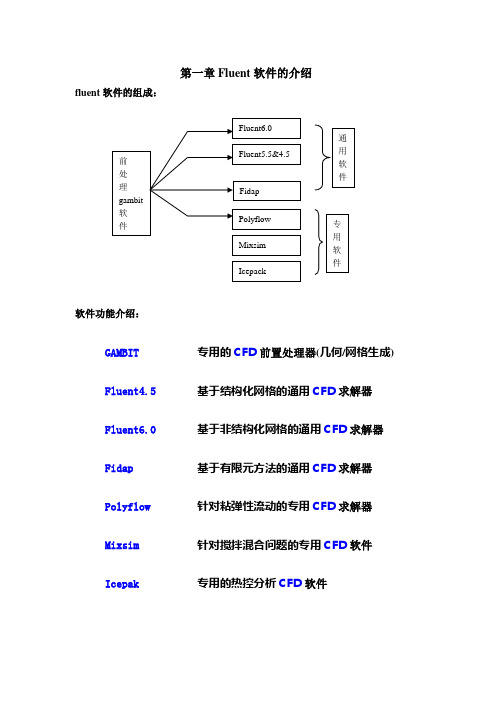
第一章Fluent 软件的介绍fluent 软件的组成:软件功能介绍:GAMBIT 专用的CFD 前置处理器(几何/网格生成) Fluent4.5 基于结构化网格的通用CFD 求解器 Fluent6.0 基于非结构化网格的通用CFD 求解器 Fidap 基于有限元方法的通用CFD 求解器 Polyflow 针对粘弹性流动的专用CFD 求解器 Mixsim 针对搅拌混合问题的专用CFD 软件 Icepak专用的热控分析CFD 软件软件安装步骤:step 1: 首先安装exceed软件,推荐是exceed6.2版本,再装exceed3d,按提示步骤完成即可,提问设定密码等,可忽略或随便填写。
step 2: 点击gambit文件夹的setup.exe,按步骤安装;step 3: FLUENT和GAMBIT需要把相应license.dat文件拷贝到FLUENT.INC/license目录下;step 4:安装完之后,把x:\FLUENT.INC\ntbin\ntx86\gambit.exe命令符拖到桌面(x为安装的盘符);step 5: 点击fluent源文件夹的setup.exe,按步骤安装;step 6: 从程序里找到fluent应用程序,发到桌面上。
注:安装可能出现的几个问题:1.出错信息“unable find/open license.dat",第三步没执行;2.gambit在使用过程中出现非正常退出时可能会产生*.lok文件,下次使用不能打开该工作文件时,进入x:\FLUENT.INC\ntbin\ntx86\,把*.lok文件删除即可;3.安装好FLUENT和GAMBIT最好设置一下用户默认路径,推荐设置办法,在非系统分区建一个目录,如d:\usersa) win2k用户在控制面板-用户和密码-高级-高级,在使用fluent用户的配置文件修改本地路径为d:\users,重起到该用户运行命令提示符,检查用户路径是否修改;b) xp用户,把命令提示符发送到桌面快捷方式,右键单击命令提示符快捷方式在快捷方式-起始位置加入D:\users,重起检查。
!!!FLUENT在气动噪声问题上的处理方法

已经发布了气动噪声模块SPL (dB):0 20 30 40 50 60 70 80 90 100 110 120Source AcousticSource Intensity, IFarfieldSurfaceSound Power = ∫IdAAcousticPressure, p(t)Pap prms µ20,log2=Frequency range (20 Hz ~ 20,000 Hz)Temporal resolution for acoustics is often orders ofTo radiate the acoustic pressure to the farfieldanalogy)Solve the flow using NS equation to capture soundAdvantages of the two step procedure Separate length scales. NS equation deals ONLY with shortSound is induced by fluid flow with its fluctuatingInclude solid surfaces and density fluctuationV i=0)Lighthill-Curle’s solution for acoustic pressureused this formulation for a rotatingThe Sears function provides a description of the unsteady aerodynamic response of a body due toCorrelate the flow parameters to noise levels.showed relations for acoustic power:CFD Acoustic Modeling OptionsOutput PhenomenaGenerate LES SolutionAirflow over a flat-plate with30 mmn Plate PlatePerform transient LES turbulent 2D analysis inAcoustic Pressure andAcoustic pressure variation with timeFor the present flow, SPL = 108 (dB))/()(2m W f p Φ)()(dB f p ΦPeak at f = 3434 HzPower Spectral DensitySurface Dipole Strengthmeasures local contribution)Local contribution to acoustic pressure can beTransient simulations can be used with Lighthill-L = 1m, D = 0.267m (L/D = 3.75)Cavity Flow MethodologyAcoustic calculationAcoustic Pressure TracesCavity Acoustic PressureSummaryUnsteady flow predicted with FLUENT is used as the source termMuffler Frequency ResponseA. J. Torregrosa, & A. Gil, Dept. of ThermalEngines, Polytechnic University of ValenciaMuffler Acoustics Methodology2D Axisymmetric, 10,000 cells3D w/ 1 Plane of Symmetry, 60,000 cellsincident wave3D Muffler Pressure IsosurfacesPressure IsoSurfaces at several frequencies f=95.15 Hz f=266.42 Hz f=342.54 Hzf=685.08 Hzf=1046.65 HzTransmission Loss CalculationsTL de TT2110016TL de TT2110016Response ConclusionsCalculation Method has been defined toWind Noise = Pressure fluctuations caused byPrimary sources of Wind Noise are•Leakage wave propagation simulated with FLUENTExamples: Door gap cavities, wiper well, cavities inPossible to qualitatively characterize source strength average flow pressure fluctuation magnitude inFlow pressure fluctuations on a solid surface in the flow cause acoustic pressure fluctuations to be radiated outTurn on UDF after transient simulation。
FLUENT官方培训教材(完整版)

Gas outlet
Oil outlet
Three- Phase Inlet
Water outlet
Contours of Oil Volume Fraction in a Three-Phase Separator
Update Model
1. 定义模拟目的
你希望得到什么样的结果(例如,压降,流量),你如何使用这些结果? 你的模拟有哪些选择? 你的分析应该包括哪些物理模型(例如,湍流,压缩性,辐射)? 你需要做哪些假设和简化? 你能做哪些假设和简化(如对称、周期性)? 你需要自己定义模型吗? FLUENT使用UDF,CFX使用 User FORTRAN 计算精度要求到什么级别? 你希望多久能拿到结果? CFD是否是合适的工具?
Solid model of a Headlight Assembly
Pre-Processing Mesh Physics Solver Settings
4. 设计和划分网格
计算域的各个部分都需要哪种程度的网格密度? 网格必须能捕捉感兴趣的几何特征,以及关心变量的梯度,如速度梯度、压力梯度、温度梯度等。 你能估计出大梯度的位置吗? 你需要使用自适应网格来捕捉大梯度吗? 哪种类型的网格是最合适的? 几何的复杂度如何? 你能使用四边形/六面体网格,或者三角形/四面体网格是否足够合适? 需要使用非一致边界条件吗? 你有足够的计算机资源吗? 需要多少个单元/节点? 需要使用多少个物理模型?
Problem Identification Identify domain
2. 确定计算域
fluent噪声培训资料(中)
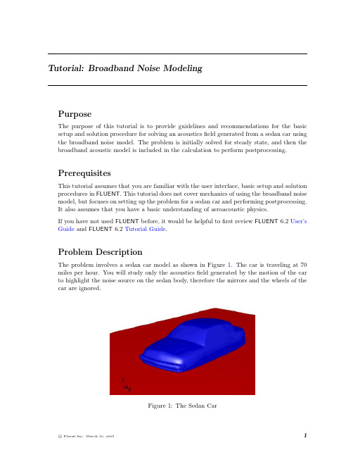
Tutorial:Broadband Noise ModelingPurposeThe purpose of this tutorial is to provide guidelines and recommendations for the basic setup and solution procedure for solving an acousticsfield generated from a sedan car using the broadband noise model.The problem is initially solved for steady state,and then the broadband acoustic model is included in the calculation to perform postprocessing.PrerequisitesThis tutorial assumes that you are familiar with the user interface,basic setup and solution procedures in FLUENT.This tutorial does not cover mechanics of using the broadband noise model,but focuses on setting up the problem for a sedan car and performing postprocessing.It also assumes that you have a basic understanding of aeroacoustic physics.If you have not used FLUENT before,it would be helpful tofirst review FLUENT6.2User’s Guide and FLUENT6.2Tutorial Guide.Problem DescriptionThe problem involves a sedan car model as shown in Figure1.The car is traveling at70 miles per hour.You will study only the acousticsfield generated by the motion of the car to highlight the noise source on the sedan body,therefore the mirrors and the wheels of the car are ignored.Figure1:The Sedan CarBroadband Noise ModelingPreparation1.Copy the meshfile,sedan-acoustics.msh from the inputfile into your working di-rectory.2.Start the3D version of FLUENT.Setup and SolutionStep1:Grid1.Read the meshfile,sedan-acoustics.msh.File−→Read−→Case...2.Check the grid.Grid−→Check...3.Keep default scale for the grid.Grid−→Scale...4.Display the grid.Display−→Grid...Figure2:Grid DisplayBroadband Noise Modeling Step2:Models1.Keep the default solver settings.Define−→Models−→Solver...2.Enable the standard k-epsilon turbulence model.Define−→Models−→Viscous...Step3:MaterialsDefine−→Materials...1.Keep the default selection of air in the Materials panel.Step4:Operating ConditionsDefine−→Operating Conditions...1.Keep the default operating conditions.Step5:Boundary ConditionsDefine−→Boundary Conditions...1.Set the boundary conditions for velocity inlet(inlet).(a)Under Zone,select inlet.The Type will be reported as velocity-inlet.(b)Click Set...to open the Velocity Inlet panel.Broadband Noise Modelingi.Specify a value of31for Velocity Magnitude.ii.Select Intensity and Length Scale in the Turbulence Specification Method drop-down list.iii.Specify a value of2and0.35for Turbulence Intensity and Turbulence Length Scale respectively.2.Set the boundary conditions for pressure outlet(outlet)as shown in the panel.3.Keep the default boundary conditions for other walls.Broadband Noise Modeling Step6:Solution1.Retain the default under-relaxation factors and discretization schemes.Solve−→Controls−→Solution...2.Enable the plotting of residuals during the calculation(Figure3).Solve−→Monitors−→Residual...3.Initialize the solution.Solve−→Initialize−→Initialize...(a)Select inlet in the Compute From drop-down list and click Init.4.Write the casefile(sedan.cas.gz).5.Start the calculation by requesting70iterations.Solve−→Iterate...6.Write the datafile(sedan.dat.gz).Broadband Noise ModelingFigure3:Scaled ResidualsStep7:Enable the Broadband Acoustic ModelDefine−→Models−→Acoustics...1.Under Model,select Broadband Noise Sources.(a)Specify a value4e-10for Reference Acoustic Power(w).(b)Set the Number of Realizations to50.Broadband Noise Modeling(c)Retain the default values for the rest of the model constants and click OK toclose the panel.Step8:Postprocessing1.Display thefilled contours of Acoustics Power Level(dB)on the surfaces of the sedancar,i.e.,front,rear,and cabinet(Figure4).Display−→Contours...(a)Under Options,select Filled.(b)Select Acoustics...and Acoustic Power Level(dB)from the Contours of drop-downlists.(c)Under Surfaces,select front,rear,and cabinet.(d)Click Display.2.Similarly,display thefilled contours of Surface Acoustics Power Level(dB)(Figure5),and Lilley’s Total Noise Source(Figure6)on the surfaces of the sedan car.Broadband Noise ModelingFigure4:Contours of Acoustic Power LevelFigure5:Contours of Surface Acoustics Power LevelBroadband Noise ModelingFigure6:Contours of Lilley’s Total Noise SourceSummaryThis tutorial demonstrated the use of FLUENT’s broadband noise acoustic model to solve an acousticsfield generated from a sedan car.You have learned how to set up the relevant parameters and postprocess the noise signals to highlight the source of noise on the sedan car body.。
fluent 噪声计算
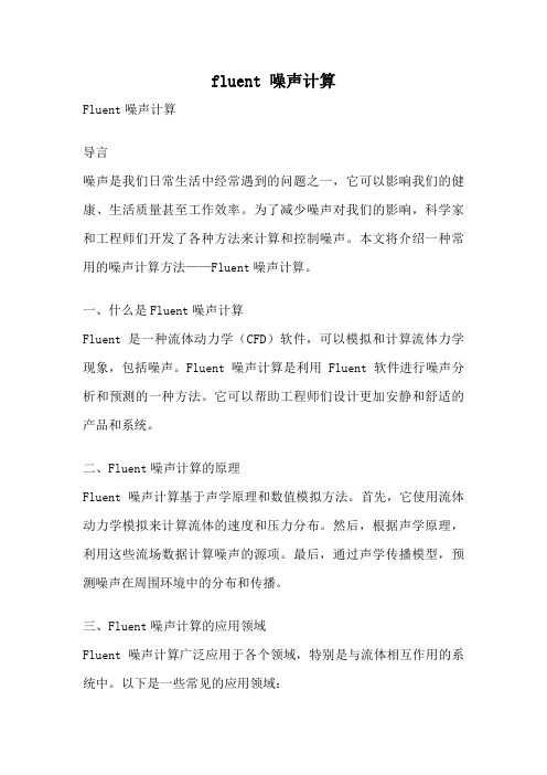
fluent 噪声计算Fluent噪声计算导言噪声是我们日常生活中经常遇到的问题之一,它可以影响我们的健康、生活质量甚至工作效率。
为了减少噪声对我们的影响,科学家和工程师们开发了各种方法来计算和控制噪声。
本文将介绍一种常用的噪声计算方法——Fluent噪声计算。
一、什么是Fluent噪声计算Fluent是一种流体动力学(CFD)软件,可以模拟和计算流体力学现象,包括噪声。
Fluent噪声计算是利用Fluent软件进行噪声分析和预测的一种方法。
它可以帮助工程师们设计更加安静和舒适的产品和系统。
二、Fluent噪声计算的原理Fluent噪声计算基于声学原理和数值模拟方法。
首先,它使用流体动力学模拟来计算流体的速度和压力分布。
然后,根据声学原理,利用这些流场数据计算噪声的源项。
最后,通过声学传播模型,预测噪声在周围环境中的分布和传播。
三、Fluent噪声计算的应用领域Fluent噪声计算广泛应用于各个领域,特别是与流体相互作用的系统中。
以下是一些常见的应用领域:1.汽车行业:Fluent噪声计算可以帮助汽车制造商设计更加安静的汽车内部和外部。
例如,可以通过优化车身外形和降低风阻来减少风噪声。
同时,通过优化排气系统和减少发动机振动,还可以降低排气噪声。
2.航空航天工业:Fluent噪声计算可以用于预测飞机和火箭发动机的噪声特性。
这对于设计更加环保和安静的飞行器至关重要。
例如,通过改进发动机设计和降低气动噪声,可以减少飞机起飞和降落时的噪声。
3.建筑和城市规划:Fluent噪声计算可以用于评估建筑物和城市规划方案的噪声影响。
例如,在设计住宅区时,可以通过优化建筑物布局和采用隔音措施,减少交通噪声对居民的影响。
四、Fluent噪声计算的优势相比传统的试验方法,Fluent噪声计算具有以下优势:1.成本效益:Fluent噪声计算可以大大降低实验成本。
传统的试验方法需要建立实验设备、采集数据并进行分析,而Fluent噪声计算只需在软件中进行模拟和计算。
(完整word版)FLUENT知识点解读(良心出品必属精品)
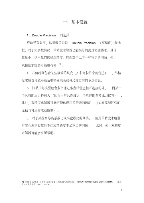
一、基本设置1.Double Precision的选择启动设置如图,这里着重说说Double Precision(双精度)复选框,对于大多数情况,单精度求解器已能很好的满足精度要求,且计算量小,这里我们选择单精度。
然而对于以下一些特定的问题,使用双精度求解器可能更有利[1]。
a.几何特征包含某些极端的尺度(如非常长且窄的管道),单精度求解器可能不能足够精确地表达各尺度方向的节点信息。
b.如果几何模型包含多个通过小直径管道相互连接的体,而某一个区域的压力特别大(因为用户只能设定一个总体的参考压力位置),此时,双精度求解器可能更能体现压差带来的流动(如渐缩渐扩管的无粘与可压缩流动模拟)。
c.对于某些高导热系数比或高宽纵比的网格,使用单精度求解器可能会遇到收敛性不佳或精确度不足不足的问题,此时,使用双精度求解器可能会有所帮助。
[1] 李鹏飞,徐敏义,王飞飞.精通CFD工程仿真与案例实战:FLUENT GAMBIT ICEM CFD Tecplot[M]. 北京,人民邮电出版社,2011:114-1162.网格光顺化用光滑和交换的方式改善网格:通过Mesh下的Smooth/Swap来实现,可用来提高网格质量,一般用于三角形或四边形网格,不过质量提高的效果一般般,影响较小,网格质量的提高主要还是在网格生成软件里面实现,所以这里不再用光滑和交换的方式改善网格,其原理可参考《FLUENT全攻略》(已下载)。
3.Pressure-based与Density-based求解器设置如图。
下面说一说Pressure-based和Density-based 的区别:Pressure-Based Solver是Fluent的优势,它是基于压力法的求解器,使用的是压力修正算法,求解的控制方程是标量形式的,擅长求解不可压缩流动,对于可压流动也可以求解;Fluent 6.3以前的版本求解器,只有Segregated Solver和Coupled Solver,其实也是Pressure-Based Solver的两种处理方法;Density-Based Solver是Fluent 6.3新发展出来的,它是基于密度法的求解器,求解的控制方程是矢量形式的,主要离散格式有Roe,AUSM+,该方法的初衷是让Fluent具有比较好的求解可压缩流动能力,但目前格式没有添加任何限制器,因此还不太完善;它只有Coupled的算法;对于低速问题,他们是使用Preconditioning方法来处理,使之也能够计算低速问题。
噪声培训资料
噪声培训资料噪声,作为一种环境污染,对人类的身体健康和生活质量都产生了不可忽视的影响。
为了更好地认识、理解和应对噪声问题,本文将介绍一些关于噪声的基本知识和常见的防噪措施。
通过培训和学习,我们可以有效地管理和减少噪声带来的负面影响。
第一章噪声的定义和分类噪声是指在特定环境中存在的、对人耳产生不愉快、甚至有害的声音。
根据噪声的来源和性质,可以将其分为以下几类:1. 工业噪声:来自工厂、机械设备、交通工具等工业活动产生的噪声。
2. 交通噪声:主要来自于道路、铁路、航空等交通工具和设施产生的噪音。
3. 社会噪声:包括商业区域、居民区域和公共场所等非工业和交通场所产生的噪音。
4. 家庭噪声:由电视、音响、家庭电器等家庭设备产生的噪音。
5. 自然噪声:来自自然界的噪音,如风声、雨声、海浪声等。
第二章噪声对人类的影响噪声污染不仅会影响人们的听觉系统,还会对身心健康产生负面影响。
噪声过大或长期暴露于噪音环境中,可能会引发以下问题:1. 听力损害:长时间暴露于高强度的噪音中会导致听力损伤,严重时可能引起永久性听力受损。
2. 神经系统问题:噪声会引起人体神经系统的紊乱,导致失眠、头痛、注意力不集中等问题。
3. 心理健康影响:持续的噪声刺激可能导致焦虑、抑郁和压力等心理问题。
4. 社交和学习问题:噪声会干扰人们的交流和学习,影响工作效率和学习成绩。
5. 心血管疾病:长期暴露于噪声环境中会增加患心血管疾病的风险,如高血压和心脏病。
第三章防噪措施的介绍为了减少噪声的影响,我们可以采取一系列防噪措施,包括以下几个方面:1. 隔音措施:通过改善建筑材料和设计结构,减少声音的传导和传播。
2. 声音吸收:使用吸音材料,如地毯、窗帘、吸音板等,减少声音的反射和回声。
3. 噪音管制:制定合理的法律法规,加强对工业、交通和社会噪声的管制和监督。
4. 个人保护措施:佩戴耳塞或耳罩,避免长时间暴露在高噪音环境中。
5. 教育宣传:提高公众对噪声问题的认识和重视,普及噪声管理的知识和技能。
FLUENT官方培训教材完整版幻灯片

100%
简化模型
在保证计算精度的前提下,合理 简化模型以降低计算量。
80%
设定边界条件
根据实际问题,设定模型的边界 条件,如入口、出口、壁面等。
网格划分策略及技巧
选择合适的网格类型
根据模型特点选择合适的网格 类型,如结构化网格、非结构 化网格等。
求解策略
采用有限体积法进行数值求解,结合适当的 湍流模型和热传导方程进行迭代计算。
结果分析
展示温度场、热流量和努塞尔数等关键结果 ,评估热设计方案的合理性。
07
总结回顾与拓展学习资源推荐
本次培训内容总结回顾
FLUENT软件基础操作
介绍了FLUENT软件界面、基本功能 、操作流程等。
前处理与网格划分
演示技巧
分享动画演示的实用技巧,如选择合适的帧率、添加背景音乐和解 说等。
输出格式
支持多种动画输出格式,如AVI、MP4等,方便在不同场合进行演 示和分享。
数据提取、导出及报告编写
数据提取
从计算结果中提取关键数据,如某点的速度、压力值等。
数据导出
将提取的数据导出为Excel、CSV等格式,便于进一步分析 和处理。
求解策略
采用有限体积法进行数值求解 ,结合湍流模型捕捉流动细节 ,提高计算精度。
结果分析
展示管道内的速度场、压力场 和流量分布等关键结果,评估
管道设计的合理性。
案例三:多相流混合过程模拟
问题描述
多相流体(如气液、气 固等)在混合过程中的 相互作用和流动特性。
建模方法
在FLUENT中建立多相 流模型,定义各相的物 理属性和相互作用机制
01-第一篇 FLUENT 基础知识
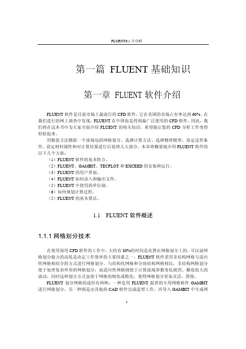
FLUENT6.1全攻略第一篇 FLUENT基础知识第一章 FLUENT软件介绍FLUENT软件是目前市场上最流行的CFD软件,它在美国的市场占有率达到60%。
在我们进行的网上调查中发现,FLUENT在中国也是得到最广泛使用的CFD软件。
因此,我们将在这本书中为大家全面介绍FLUENT的相关知识,希望能让您的CFD分析工作变得轻松起来。
用数值方法模拟一个流场包括网格划分、选择计算方法、选择物理模型、设定边界条件、设定材料属性和对计算结果进行后处理几大部分。
本章将概要地介绍FLUENT软件的以下几个方面:(1)FLUENT软件的基本特点。
(2)FLUENT、GAMBIT、TECPLOT和EXCEED的安装和运行。
(3)FLUENT的用户界面。
(4)FLUENT如何读入和输出文件。
(5)FLUENT中使用的单位制。
(6)如何规划计算过程。
(5)FLUENT的基本算法。
1.1FLUENT软件概述1.1.1网格划分技术在使用商用CFD软件的工作中,大约有80%的时间是花费在网格划分上的,可以说网格划分能力的高低是决定工作效率的主要因素之一。
FLUENT软件采用非结构网格与适应性网格相结合的方式进行网格划分。
与结构化网格和分块结构网格相比,非结构网格划分便于处理复杂外形的网格划分,而适应性网格则便于计算流场参数变化剧烈、梯度很大的流动,同时这种划分方式也便于网格的细化或粗化,使得网格划分更加灵活、简便。
FLUENT划分网格的途径有两种:一种是用FLUENT提供的专用网格软件GAMBIT 进行网格划分,另一种则是由其他的CAD软件完成造型工作,再导入GAMBIT中生成网1FLUENT6.1全攻略格。
还可以用其他网格生成软件生成与FLUENT兼容的网格用于FLUENT计算。
可以用于造型工作的CAD软件包括I-DEAS、Pro/E、SolidWorks、Solidedge等。
除了GAMBIT 外,可以生成FLUENT网格的网格软件还有ICEMCFD、GridGen等等。
Fluent计算远场噪声设置
Fluent计算远场噪声设置XXX远场噪声FW-H声比计算设置Fluent可以准确地计算偶极子壁面积分的远场噪声,并且可以计算其他类型的声源积分面。
1)设置求解器首先打开Fluent。
在计算之前,需要设置并行核数与电脑相同,以及当前文件路径和是2D还是3D。
等到计算基本稳定后,开始打开声学模块采样计算。
可以通过观察升阻力系数曲线或流动出口质量流量等指标来判断流动周期是否稳定,当曲线上下波动时可以开始计算,例如在0.2时。
打开声学求解器,空气参数默认不需改动,勾选输出ASD和CGNS格式。
打开define sources,选择需要积分计算的壁面边界条件,给文件名、写入频率和多少个时间步一个文件保存。
如果需要积分超声速的空间四极子噪声,需要设置interface自由空间边界条件或导出数据到其他声学软件,速度不是特别大的情况下可以忽略。
define receivers观测点位置可以在任何时候设置。
2)FFT后处理时域数据计算完噪声后,打开run n里面的Acoustic signals,点击Compute开始计算。
观测点计算完之后,点击XY Plot,选择所有类型,在最后打开观测点的.ard文件的格式读取、计算和显示观测点随着时间变化的曲线,处于上下波动的状态用FFT 转化到频域。
点击Load Input Files读入观测点时间的数据,点击Acoustics Analysis,选择SPL声压级,将横坐标改为log分布,并关闭Auto自动,手动给横坐标范围分块加汉宁窗对曲线进行改进,勾选Subdivide into Segments分块,窗口选择hanning或其他类型,分块可以用sample或Frequencty,分块采样数看着给,分成4~10块,看具体实验数据的横坐标频率分辨率是多少对应,每块overlap重叠在到1之间。
点击apply。
close,点击Plot FFT就得到频谱曲线。
湍流及气动噪声仿真培训

•
Correlation based model
– – –
Reasonably accurate Correlations can be found for many different transition mechanisms (e.g. FSTI, dp/dx, Roughness) Not compatible with 3D flows and unstructured/parallel CFD codes – non-local formulation
transitional flows
如何选择合适的湍流模型?
rotating & swirling flows crossflow/secondary flows thin shear flows separated & recirculating flows rapidly strained flows
Modelling
• Numerous developments: – Correlation based models – Low-Re models – en linear stability – … – DNS
Almost all industrial CFD simulations are calculated without a transition model
声比拟模型fwh特点噪声比拟方法不同于caa方法它把波动方程和流动方程解耦在近场流动解析采用适当的控制方程比如非定常雷诺平均des分离涡或les大涡模拟等方法然后再把求解结果作为噪声源通过求解波动方程得到解析解这样就把流动求解过程从声学分析中分离出来
ANSYS CFD 湍流模型 及流动噪声高级应用培训
fluent噪声培训资料(上)
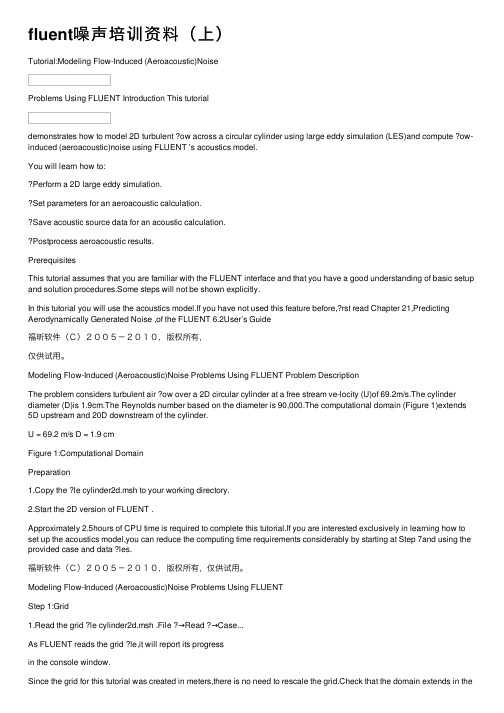
fluent噪声培训资料(上)Tutorial:Modeling Flow-Induced (Aeroacoustic)NoiseProblems Using FLUENT Introduction This tutorialdemonstrates how to model 2D turbulent ?ow across a circular cylinder using large eddy simulation (LES)and compute ?ow-induced (aeroacoustic)noise using FLUENT ’s acoustics model.You will learn how to:Perform a 2D large eddy simulation.Set parameters for an aeroacoustic calculation.Save acoustic source data for an acoustic calculation.Postprocess aeroacoustic results.PrerequisitesThis tutorial assumes that you are familiar with the FLUENT interface and that you have a good understanding of basic setup and solution procedures.Some steps will not be shown explicitly.In this tutorial you will use the acoustics model.If you have not used this feature before,?rst read Chapter 21,Predicting Aerodynamically Generated Noise ,of the FLUENT 6.2User’s Guide福昕软件(C)2005-2010,版权所有,仅供试⽤。
fluent气动噪声算例-Flow-Induced (Aeroacoustic) Noise

Tutorial:Modeling Flow-Induced(Aeroacoustic)Noise Problems Using FLUENTIntroductionThis tutorial demonstrates how to model2D turbulentflow across a circular cylinder using large eddy simulation(LES)and computeflow-induced(aeroacoustic)noise using FLUENT’s acoustics model.You will learn how to:•Perform a2D large eddy simulation.•Set parameters for an aeroacoustic calculation.•Save acoustic source data for an acoustic calculation.•Calculate acoustic pressure signals.•Postprocess aeroacoustic results.PrerequisitesThis tutorial assumes that you are familiar with the FLUENT interface and that you have a good understanding of basic setup and solution procedures.Some steps will not be shown explicitly.In this tutorial you will use the acoustics model.If you have not used this feature before,first read Chapter21,Predicting Aerodynamically Generated Noise,of the FLUENT6.2 User’s GuideModeling Flow-Induced(Aeroacoustic)Noise Problems Using FLUENTProblem DescriptionThe problem considers turbulent airflow over a2D circular cylinder at a free stream ve-locity(U)of69.2m/s.The cylinder diameter(D)is1.9cm.The Reynolds number based on the diameter is90,000.The computational domain(Figure1)extends5D upstream and 20D downstream of the cylinder.U = 69.2 m/s D = 1.9 cmFigure1:Computational DomainPreparation1.Copy thefile cylinder2d.msh to your working directory.2.Start the2D version of FLUENT.Approximately2.5hours of CPU time is required to complete this tutorial.If you are interested exclusively in learning how to set up the acoustics model,you can reduce the computing time requirements considerably by starting at Step7and using the provided case and datafiles.Modeling Flow-Induced(Aeroacoustic)Noise Problems Using FLUENT Step1:Grid1.Read the gridfile cylinder2d.msh.File−→Read−→Case...As FLUENT reads the gridfile,it will report its progress in the console window.Since the grid for this tutorial was created in meters,there is no need to rescale the grid.Check that the domain extends in the x-direction from-0.095m to0.38m.2.Check the grid.Grid−→CheckFLUENT will perform various checks on the mesh and will report the progress in the console window.Pay particular attention to the reported minimum volume.Make sure this is a positive number.3.Reorder the grid.Grid−→Reorder−→DomainTo speed up the solution procedure,the mesh should be reordered,which will substan-tially reduce the bandwidth and make the code run faster.FLUENT will report its progress in the console window:>>Reordering domain using Reverse Cuthill-McKee method:zones,cells,faces,done.Bandwidth reduction=32634/253=128.99Done.Modeling Flow-Induced(Aeroacoustic)Noise Problems Using FLUENT4.Display the grid.Display−→Grid...(a)Display the grid with the default settings(Figure2).Use the middle mouse button to zoom in on the image so you can see the meshnear the cylinder(Figure3).Figure2:Grid DisplayModeling Flow-Induced(Aeroacoustic)Noise Problems Using FLUENTFigure3:The Grid Around the CylinderQuadrilateral cells are used for this LES simulation because they generate less numerical diffusion than triangular cells.The cell size should be small enough to capture the relevant turbulence length scales,and to make the numerical diffusion smaller than the subgrid-scale turbulence viscosity.The mesh for this tutorial has been kept coarse in order to speed up the calculations.A high quality LES simulation will require afiner mesh near the cylinder wall.Modeling Flow-Induced(Aeroacoustic)Noise Problems Using FLUENT Step2:Models1.Select the segregated solver with second-order implicit unsteady formulation.Define−→Models−→Solver...(a)Retain the default selection of Segregated under Solver.(b)Under Time,select Unsteady.(c)Under Transient Controls,select Non-Iterative Time Advancement.(d)Under Unsteady Formulation,select2nd-Order Implicit.(e)Under Gradient Option,select Node-Based.(f)Click OK.Modeling Flow-Induced(Aeroacoustic)Noise Problems Using FLUENT2.Select the LES turbulence model.The LES turbulence model is not available by default for2D calculations.You can make it available in the GUI by typing the following command in the FLUENT console window:(rpsetvar’les-2d?#t)Define−→Models−→Viscous...(a)Under Model,select Large Eddy Simulation.(b)Retain the default option of Smagorinsky-Lilly under Subgrid-Scale Model.(c)Retain the default value of0.1for the model constant Cs.(d)Click OK.You will see a Warning dialog box,stating that Bounded Central-Differencing is default for momentum with LES/DES.Click OK.The LES turbulence model is recommended for aeroacoustic simulations because LES resolves all eddies with scales larger than the grid scale.Therefore,wide band aeroa-coustic noise can be predicted using LES simulations.Modeling Flow-Induced(Aeroacoustic)Noise Problems Using FLUENTStep3:MaterialsYou will use the default material,air,which is the workingfluid in this problem.The default properties will be used for this simulation.Define−→Materials...1.Retain the default value of1.225for Density.2.Retain the default value of1.7894e-05for Viscosity.You can modify thefluid properties for air or copy another material from the database if needed.For details,refer the chapter Physical Poperties in the FLUENT User’s Guide.Step4:Operating ConditionsDefine−→Operating Conditions...1.Retain the default value of101325Pa for the Operating Pressure.Step5:Boundary Conditions1.Retain the default conditions for thefluid.Define−→Boundary Conditions...(a)Under Zone,selectfluid.The Type will be reported asfluid.(b)Click Set...to open the Fluid panel.i.Retain the default selection of air as thefluid material in the Material Namedrop-down list.ii.Click OK.2.Set the boundary conditions at the inlet.(a)Under Zone,select inlet.The Type will be reported as velocity-inlet(b)Click Set...to open the Velocity Inlet panel.i.Set the Velocity Magnitude to69.2m/s.ii.Retain the default No Perturbations in the Fluctuating Velocity Algorithm drop-down list,and click OK..This tutorial does not make use of FLUENT’s ability to impose inlet pertur-bations at velocity inlets when using LES.It is assumed that all unsteadinessis due to the presence of the cylinder in theflow.Modeling Flow-Induced(Aeroacoustic)Noise Problems Using FLUENT3.Set the boundary conditions at the outlet.(a)Under Zone,select outlet.The Type will be reported as pressure-outlet(b)Click Set...to open the Pressure Outlet panel.i.Confirm that the Gauge Pressure is set to0.ii.Retain the default option of Normal to Boundary in the Backflow Direction Specification Method drop-down list,and click OK.The top and bottom boundaries are set to symmetry boundaries.No user input is required for this boundary type.Step6:Quasi-Stationary Flow Field SolutionBefore extracting the source data for the acoustic analysis,a quasi-stationaryflow needs to be established.The quasi-stationary state will be judged by monitoring the lift and drag forces.1.Set the solution controls.Solve−→Controls−→Solution...(a)Retain the default PISO scheme for Pressure-Velocity Coupling.(b)Under Discretization,select PRESTO!in the Pressure drop-down list.PRESTO!is a more accurate scheme for interpolating face pressure values fromcell pressures.Modeling Flow-Induced(Aeroacoustic)Noise Problems Using FLUENT(c)Retain the default Bounded Central Differencing for Momentum.For LES calculations on unstructured meshes,the Bounded Central Differencingscheme is recommended for Momentum.(d)Set the Relaxation Factor for Pressure to0.75.(e)Retain the default Relaxation Factor for Momentum.The pressurefield is relaxed only during the initial transient phase.The Relax-ation Factor for Pressure will be increased to1at a later stage.(f)Click OK.2.Initialize the solution.Solve−→Initialize−→Initialize...(a)Initialize theflow from the inlet conditions by selecting inlet in the Compute Fromdrop-down list.(b)Click Init to initialize the solution and click Close.3.Enable the plotting of residuals.Solve−→Monitors−→Residual...(a)Select Plot under Options.(b)Under Storage,enter10000Iterations.(c)Under Plotting,enter20Iterations.(d)Retain the default values for the other parameters and click OK.4.Set the time step parameters.Solve−→Iterate...(a)Set the Time Step Size(s)to5e-6.The time step size required in LES calculations is governed by the time scaleof the smallest resolved eddies.That requires the local Courant-Friedrichs-Lewy(CFL)number to be of an order of1.It is generally difficult to know the propertime step size at the beginning of a simulation.Therefore,an adjustment aftertheflow is established,is often necessary.For a given time step∆t,the highestfrequency that the acoustic analysis can produce is f=12∆t .For the time step sizeselected here,the maximum frequency is100kHz.Typically in most aeroacoustic calculations,the maximum frequency obtained from the analysis is higher than the audible range of interest.(b)Click Apply.5.Save the case and datafiles(cylinder2d t0.00.cas.gz and cylinder2d t0.00.dat.gz).File−→Write−→Case&Data...Save the case and datafiles before thefirst iteration.This will save you time in the event of user error or code divergence,where the casefile would have to be set up all over again.6.Run the case for a few time steps before activating the force monitors.Solve−→Iterate...(a)Set the Number of Time Steps to20.(b)Click Iterate.The residual history will be displayed as the calculation proceeds.When the non-iterative time advancement scheme is used,by default,two residuals are plotted per time step.7.Enable the monitoring of the lift and drag forces.Setting the force monitors after some initial transient state limits the range of the drag coefficient when starting from an impulse initial condition.Solve−→Monitors−→Force...(a)In the Coefficient drop-down list,select Drag.(b)In the Wall Zones list,select wall cylinder.(c)Verify that the X and Y values under Force Vector are1and0,respectively.(d)Under Options,select Plot to enable plotting of the drag coefficient.(e)Under Options,select Write to save the monitor history to afile,cd-history willbe the defaultfile name.If you do not select the Write option,the history information will be lost when you exit FLUENT.(f)Click Apply.(g)In the Coefficient drop-down list,select Lift.(h)Under Force Vector,specify X and Y to be0and1,respectively.(i)Under Options,select Plot to enable plotting of the lift coefficient.(j)Under Options,select Write to save the monitor history to afile.This time, cl-history will be the defaultfile name.(k)Close the panel.8.Set the reference values to be used in the lift and drag coefficient calculation.Report−→Reference Values...(a)Set the values as shown in the table:Parameter ValueArea0.019Velocity69.2Length0.019(b)Retain the default values for the other parameters and click OK.The reference area is calculated using the cylinder diameter,D,and the default depth of1m for2D problems.Adjust the reference area if a different depth (Depth)value is used.For the actual force coefficient calculation,only the reference area,density and velocity are needed.The reference length(Length)will be needed later for the Strouhal number calculation.9.Overwrite the previously saved initial conditions(cylinder2d t0.00.cas.gz andcylinder2d t0.00.dat.gz).File−→Write−→Case&Data...10.Advance theflow in time until a quasi-stationary state is reached.Solve−→Iterate...(a)Set the Number of Time Steps to4000.(b)Click Iterate.The4000time steps will advance theflow up to t=0.02s.At that time the bulkflow will have crossed the computational domain about three times.The residual history,lift and drag force histories will be displayed as the calculation proceeds.The lift and drag histories should be similar to Figure4and Figure5, respectively.Differences in the long-termflow evolution can occur due to operating system dependent round-offerrors.Once the lift and drag histories are sufficiently oscillatory and periodic in nature,you are ready to set up the acoustics model and perform the acoustic calculations.Figure4:Lift Coefficient History11.Verify that the selected time step size is reasonable for the given mesh andflowcondition.Plot−→Histogram...Figure5:Drag Coefficient History(a)Under Histogram of,select Velocity....(b)From the Velocity...category,select Cell Courant Number.(c)Set the value for Divisions to100.(d)Click Plot and verify that the peak CFL value is less than3.5.The histogram(Figure6)shows that most cells have a Cell Courant Number of less than1.12.Save the case and datafiles(cylinder2d t0.02.cas.gz and cylinder2d t0.02.dat.gz).File−→Write−→Case&Data...Figure6:A Histogram Displaying the Range of the CFL Number Step7:Aeroacoustics Calculation1.Define the acoustics model settings.Define−→Models−→Acoustics...(a)Under Model,select Ffowcs-Williams&Hawkings.(b)Under Options,select Export Acoustic Source Data.(c)Click the Sources...button.This will open the Acoustic Sources panel.i.Under Source Zones,select wall cylinder.All relevant acoustic source data(i.e.pressure in this case)will be extracted from the wall cylinder surface.ii.In the text-entry box for Source Data Root Filename,enter cylinder2d.This is thefilename root of the indexfile which will be created.The index file contains information about the source datafiles that are created when you run the case.The indexfile is automatically created with a.indexfile extension.iii.Under Write Frequency,enter2.Depending on the physical time step size and the important time scales in theflow,it is not necessary to write the acoustic source data at every time step.In this tutorial,the source data is coarsened(in time)by a factor of two.Thus,the highest possible frequency the acoustic analysis can generate is reduced to f=1=50kHz.2(2∆t)iv.Set the No.of Time Steps Per File to200.The source data can be conveniently segmented into multiple source data files.This makes it easier to process partial sequences when calculating the receiver signals.A value of200for No.of Time Steps Per File means that each source datafile covers a time span of200time steps.With a Write Frequency of2,there are100data sets written into each source datafile.v.Click Apply and Close.(d)Click OK to close the Acoustics Model panel.2.Modify the solution controls.Solve−→Controls−→Solution...(a)Increase the Relaxation Factor for Pressure to1.(b)Click OK.3.Resume the calculation.Solve−→Iterate...(a)Retain the Number of Time Steps at4000.(b)Click Iterate.The additional4000time steps will advance theflow up to t=0.04s.At every second time step,a message will be displayed in the FLUENT console window informing you that data is written to a source datafile(.asdfile extension).4.Save the case and datafiles(cylinder2d t0.04.cas.gz and cylinder2d t0.04.dat.gz).File−→Write−→Case&Data...5.Set the acoustics model constants.Define−→Models−→Acoustics...(a)Retain the Far-Field Density at1.225kg/m3.The far-field density is the density of thefluid outside the computational domain,i.e.the density of thefluid near the receivers.In most calculations it is the sameas the density within the computational domain.(b)Use the default value of340m/s for the Far-Field Sound Speed.(c)Leave the Reference Acoustic Pressure at2e-05Pa.The reference acoustic pressure is used to calculate decibel values during postpro-cessing.(d)Set the Source Correlation Length to0.095m.That is equal tofive cylinderdiameters.The source correlation length is very important when performing aeroacoustic cal-culations in2D.FLUENT assumes that the sound sources are perfectly correlatedover the specified correlation length,and zero outside.That is,FLUENT internallybuilds a source volume with a depth equal to the specified correlation length andneglects sources outside.In your practical2D application,you will have to esti-mate the source correlation length;your obtained sound pressure levels will de-pend on your input.That makes it difficult to rely on2D calculations to obtainabsolute sound pressure levels.Therefore,you should use aeroacoustic2D simu-lations primarily to observe trends.The source correlation length is not neededfor3D calculations.(e)Click OK to close the panel.6.Calculate the acoustic signals.Solve−→Acoustic Signals...(a)Click the Receivers...button.This will open the Acoustic Receivers panel.Note that you can open the Acoustic Receivers panel also from the Acoustics Model and Acoustic Sources panels.i.Increase the No.of Receivers to2.ii.For the receiver-1coordinates,enter0m for X-Coord.,-0.665m(35D)for Y-Coord.,and0for Z-Coord.iii.For the receiver-2coordinates,enter0m for X-Coord.,-2.432m(128D)for Y-Coord.,and0for Z-Coord.iv.Retain the defaults for Signal File Name(receiver-1.ard and receiver-2.ard).v.Click OK to close the Acoustic Receivers panel.(b)Under Active Source Zones,select wall cylinder.All source zones which were selected in the Acoustic Sources panel are now avail-able under the Active Source Zones.In this tutorial,the sound sources are ex-tracted from only one zone.It is important to select the source zones consistentlyif redundant source zones were selected in the Acoustic Sources panel.(c)Under Source Datafiles,select allfiles available.Selecting a subset of the available sourcefiles is a convenient way to analyzeshorter sequences.It is important to select a contiguous set of source datafiles.(d)Under Receivers,select the two available receivers.As soon as the source zones,source datafiles,and receivers are selected,theCompute/Write function becomes available.(e)Click Compute/Write.The FLUENT console window will confirm that the source datafiles are beingread and that the receiver signals are computed and written into receiverfiles.(f)Click Close to close the Acoustic Signals panel.Step8:Aeroacoustic Postprocessing1.Display the acoustic pressure signals at the two receiver locations.Plot−→File...(a)Click Add...in the File XY Plot panel.This will open the Select File panel where you can now select receiver-1.ardand receiver-2.ard from the Files list.(b)Click OK to close the Select File panel.(c)Click Plot to display the receiver signals(Figure7).Modify the line and markerstyles as necessary,using the Curves panel.You will notice a shift in time of approximately5e-3s for the signal at the second receiver.Receiver-2is farther away from the source surface and the sound will therefore arrive later.Also notice that the signal at receiver-2is weaker due to the increased distance and geometrical attenuation.Figure7:Acoustic Pressure Signals2.Perform a spectral analysis of the receiver signals.Plot−→FFT...(a)Under Process Options,select Process Receiver.This will activate the Receiverlist.If the Ffowcs Williams and Hawkings(FW-H)acoustics model is used and the receiver signals have been calculated,then the signals are directly available for postprocessing.As an alternative,the receiver data can be loaded manually from files by using the Process File Data option under Process Options.(b)Select receiver-1from the Receiver list.(c)Select Sound Pressure Level(dB)from the Y Axis Function drop-down list.(d)Select Frequency(Hz)from the X Axis Function drop-down list.(e)Click Plot FFT to plot the sound pressure spectrum for receiver-1(Figure8).The overall sound pressure level(OASPL)is printed to the FLUENT console window:>>Overall Sound Pressure Levelin dB(reference pressure=2.000000e-05)=1.156790e+02=50kHz,as expected.Note that the maximum frequency plotted is f=12(2∆t)Figure8:Spectral Analysis of Pressure Signal for receiver-1(f)Click Axes....This will open the Axes-Fourier Transform panel.i.Deselect Auto Range for the X Axis.ii.Manually set the Maximum for Range to5000.iii.Click Apply and Close the panel.(g)Replot the sound pressure spectrum for receiver-1.The spectrum peaks at about900Hz(Figure9).Note that the spectral resolution is only about50Hz,since the receiver signal was calculated for a short period only(approximately0.02s).For a sampled signal oflength T,the spectral resolution is1T .You may increase the spectral resolutionby running the simulation longer in time before recalculating the receiver signals.(h)Select the Strouhal Number from the X Axis Function drop-down list.i.Reset the Maximum for the x-axis Range to1,in the Axes-Fourier Transformpanel.(i)Replot the sound pressure spectrum as a function of the Strouhal Number.Thespectrum peaks at a Strouhal Number of about0.25(Figure10).If the Strouhal number calculation does not seem correct,verify that the correct values are specified in the Reference Values panel.(j)Repeat the spectral analysis for receiver-2by selecting receiver-2from the Receiver list.You should expect an OASPL of about104dB for receiver-2.3.Plot the power spectral density of the lift force history to see that the observed peaksin the receiver spectra match the dominant frequency in the lift force history.(a)Under Process Options,select Process File Data.(b)Click Load Input File...and select the lift monitorfile(cl-history).(c)Select Power Spectral Density from the Y Axis Function drop-down list.Figure9:Spectral Analysis of Pressure Signal for receiver-1at a Reduced Frequency RangeFigure10:Spectral Analysis of Pressure Signal for receiver-1as a Function of Strouhal Numbers(d)Under X Axis Function,select Strouhal Number.(e)Verify that the Maximum for the x-axis Range in the Axes-Fourier Transformpanel is1.(f)Click Plot/Modify Input Signal...to open the Plot/Modify Input Signal panel.Thispanel lets you modify and plot the signal before the Fourier Transform is applied.i.Select Clip to Range and set the Min value for X Axis Range to0.02.Without clipping the temporal range,the complete lift monitor history wouldbe analyzed including the initial transient state leading up to the quasi-stationary state.ii.Click Apply/Plot and Close to return to the Fourier Transform panel.Since the x-axis range was manually set for the spectral plot,you will not see the proper range when plotting the modified signal.You will need to temporarily reset the range if you want to plot the input signal.(g)Click Plot FFT to plot the power spectral density for the lift monitor history(Figure11).The spectrum peaks at a Strouhal number of about0.25.As indicated in Step7,2D aeroacoustic predictions depend strongly on the selected source correlation length.As a consequence,the results can befine-tuned to be in better agreement with experimental data.4.You can repeat the calculation of the acoustic signals for the additional source corre-lation lengths of2.5D and10D,using Step7as a starting point.Table1compares the obtained OASPL values with experimental values reported by Revell et al.[1].Reasonable agreement is found for correlation lengths2.5D and5D.Figure11:Spectral Analysis of Lift Force HistoryTable1:Dependence of the Predicted OASPL on the Specified Source Correlation Lengths (L=2.5D,5D,10D)2.5D5D10D Experimental Resultsreceiver-1109.7115.7121.6117receiver-298.4104.4110.4100SummaryThis tutorial demonstrated the use of FLUENT’s acoustics model to calculate the far-field sound signals generated by theflow over a2D cylinder.You have learned how to set up the relevant parameters,save the acoustic source data,calculate,and postprocess the acoustic pressure signals.The main computational efforts are spent calculating the time dependent turbulentflow. It is therefore advisable to export the sound sources during theflow calculation.This allows you to recalculate the acoustic signals for different receivers or model parameters with minimal computational costs.The tutorial demonstrated the use of the Ffowcs Williams and Hawkings acoustics tool on a2D case.You have seen that it is difficult to obtain absolute SPL predictions in2D due to the need to estimate the correlation length of the turbulentflow structures in the spanwise direction.This difficulty does not exist when solving3D acoustics problems. References1.Revell,J.D.,Prydz,R.A.,and Hays,A.P.,“Experimental Study of Airframe Noise vs.Drag Relationship for Circular Cylinders,”Lockheed Report28074,Feb.1977.Final Report for NASA Contract NAS1-14403.。
噪声培训课件

社会生活噪声治理案例
治理措施
加强物业管理,限制高声源活动时间 ,推广低噪声生活方式
治理效果
减少居民区噪声扰民现象,提高居民 生活质量
CHAPTER 06
噪声培训总结与展望
培训内容回顾与总结
噪声基本概念
深入了解了噪声的定义、分类 、来源及其对生活和工作的影
响。
噪声测量与评估
响。
合理布局
将高噪声设备远离接收者的工作和 生活区域,减少噪声对接收者的干 扰。
宣传教育
加强噪声危害的宣传教育,提高接 收者的自我保护意识。
CHAPTER 04
噪声法规与标准解读
国家相关法规政策
《中华人民共和国环境噪声污染防治法》
01
规定了环境噪声污染防治的监督管理、污染防治措施、法律责
任等方面的内容。
04
对测量数据进行处理和 分析,得出评价结果。
评价标准及指标
01
02
03
04
声压级
衡量声音大小的物理量,以分 贝(dB)为单位表示。
等效连续A声级
用于评价连续噪声的烦扰程度 ,以Leq表示。
最大声级
用于评价噪声的峰值水平,以 Lmax表示。
噪声暴露量
用于评价噪声对人体健康的影 响程度,以噪声剂量表示。
治理措施
采用隔声罩、消声器、减振器等综合治理手段,降低噪声传播和 辐射
工业噪声治理案例
治理效果
厂界噪声达标,改善工人作业环境
案例二
某化工厂噪声治理
噪声来源
压缩机、泵类等设备
工业噪声治理案例
治理措施
对设备采取隔声、吸声、减振等措施,同时对管道进行消声处理
fluent 噪声计算

fluent 噪声计算Fluent噪声计算是一种用于模拟和预测噪声传播的工程软件。
本文将介绍Fluent噪声计算的原理、应用场景以及其在工程设计中的重要性。
我们来了解一下Fluent噪声计算的原理。
Fluent噪声计算基于有限元法和声学理论,通过对流体流动的数值模拟来计算噪声的产生、传播和衰减过程。
它可以模拟各种流动噪声,包括气体流动噪声、水流噪声以及机械振动噪声等。
Fluent噪声计算的应用场景非常广泛。
在航空航天领域,它可以用于预测飞机发动机的噪声辐射和传播,帮助设计更安静的发动机。
在汽车工程中,它可以用于优化汽车外壳的设计,降低车内的噪声水平。
在工业设备设计中,它可以用于减少机器运行时的噪声,提高工作环境的舒适度。
Fluent噪声计算在工程设计中的重要性不言而喻。
首先,它可以帮助工程师在设计初期就对噪声进行预测和评估,避免在后期需要进行昂贵的修改和改进。
其次,它可以帮助工程师找到噪声产生的主要源头,从而有针对性地采取措施来降低噪声水平。
此外,Fluent 噪声计算还可以帮助工程师进行优化设计,找到噪声与其他设计参数之间的最佳平衡点。
除了以上应用场景,Fluent噪声计算还可以在城市规划和环境保护领域发挥重要作用。
通过对城市交通流动和建筑物布局进行噪声计算,可以帮助规划者合理规划道路和建筑物的位置,减少城市噪声对居民生活的影响。
此外,Fluent噪声计算还可以用于评估工厂、发电厂等工业设施对周围环境的噪声影响,保护自然生态和居民生活环境。
Fluent噪声计算是一种强大的工程软件,具有广泛的应用价值。
它可以帮助工程师预测和评估噪声,找到噪声源头,并进行优化设计,从而降低噪声水平。
在航空航天、汽车工程、工业设备设计以及城市规划等领域,Fluent噪声计算都发挥着重要的作用,为工程师提供了可靠的噪声控制解决方案。
通过合理利用Fluent噪声计算,我们可以创造更安静、更舒适的工作和生活环境。