Semantic-Trajectories-Modeling-and-Analysis

合集下载

基于两维图论聚类的中原城市群“三生”功能评估

基于两维图论聚类的中原城市群“三生”功能评估贾琦1，刘毅洁1，尹泽凯2*，张超玉1，燕宏宇1（1.郑州轻工业大学艺术设计学院，河南郑州450002；2.山东建筑大学艺术学院，山东济南250101)摘要：基于“三生”功能的现状并对其多功能性合理分区，对于促进城市群国土空间高质量发展具有重要意义。

以中原城市群为例，通过建立“三生”功能评价体系，探讨“三生”功能演化过程，运用两维图论聚类对国土空间进行分区优化。

结果表明：生产、生活功能高值位于郑州-洛阳和郑州-许昌等城市连片区并不断持续扩张，生态功能高值多集中在豫西山区；“三生”功能具有明显集聚特征，1980—2020年，中东部生产功能持续降低且呈破碎化趋势，生活功能不断聚集在各地市建成区周边并持续胁迫生态功能区域；根据两维图论聚类方法划分为5个功能区，并针对不同分区特征提出相应管控策略。

关键词：“三生”功能；分区优化；两维图论；中原城市群中图分类号：P208文献标志码：B文章编号：1672-4623（2024）04-0001-04Production-living-ecological Functional Evaluation of Central Henan UrbanAgglomeration Based on Two-dimensional Graph Theory ClusteringJIA Qi 1,LIU Yijie 1,YIN Zekai 2,ZHANG Chaoyu 1,YAN Hongyu 1(1.School of Art and Design,Zhengzhou University of Light Industry,Zhengzhou 450002,China;2.School of Art,Shandong Jianzhu University,Jinan 250101,China)Abstract:Based on the present situation of production-living-ecological function and rationally dividing it,its versatility is of great significance for promoting the high-quality development of urban agglomeration land space.Taking the Central Henan urban agglomeration for example,we discussed the evolution process of urban agglomeration production-living-ecological function by establishing the production-living-ecological function evaluation system and optimizing the territorial space based on two-dimensional graph theory clustering.The results show that ①the high value of production and living functions is located in the contiguous areas of Zhengzhou-Luoyang,Zhengzhou-Xuchang and other cities and continues to expand,while the high value of ecological function is mainly concentrated in the mountains of western Henan.②The production-liv-ing-ecological function has obvious gathering characteristics.From 1980to 2020,the production function in the mid-east area continued to de-cline and showed a trend of fragmentation,and the living function continued to gather around the urban built-up areas and continued to stress the ecological function areas.③According to the two-dimensional graph theory clustering method,it is divided into five functional zones.According to the characteristics of different zones,Corresponding management and control strategies are proposed.Key words:production-living-ecological function,zoning optimization,two-dimensional graph theory,Central Henan urban agglomeration土地功能分区是依据地域差异特征，根据多种客观实体要素及其利用方式，将特定地区的土地划分成不同区域的过程。

Time dependent vehicle routing problem with a multi ant colony system

Time dependent vehicle routing problemwith a multi ant colony systemAlberto V.Donati *,Roberto Montemanni,Norman Casagrande,Andrea E.Rizzoli,Luca M.GambardellaIstituto Dalle Molle di Studi sull’Intelligenza Artiﬁciale (IDSIA),Galleria 2,6928Manno,SwitzerlandReceived 1June 2005;accepted 1June 2006Available online 18October 2006AbstractThe Time Dependent Vehicle Routing Problem (TDVRP)consists in optimally routing a ﬂeet of vehicles of ﬁxed capac-ity when travel times are time dependent,in the sense that the time employed to traverse each given arc,depends on the time of the day the travel starts from its originating node.The optimization method consists in ﬁnding solutions that min-imize two hierarchical objectives:the number of tours and the total travel time.Optimization of total travel time is a continuous optimization problem that in our approach is solved by discretizing the time space in a suitable number of subspaces.New time dependent local search procedures are also introduced,as well as conditions that guarantee that feasible moves are sought for in constant time.This variant of the classic Vehicle Routing Problem is motivated by the fact that in urban contexts variable traﬃc con-ditions play an essential role and can not be ignored in order to perform a realistic optimization.In this paper it is shown that when dealing with time constraints,like hard delivery time windows for customers,the known solutions for the classic case become unfeasible and the degree of unfeasibility increases with the variability of traﬃc conditions,while if no hard time constraints are present,the classic solutions become suboptimal.Finally an application of the model to a real case is presented.The model is integrated with a robust shortest path algo-rithm to compute time dependent paths between each customer pairs of the time dependent model.Ó2006Elsevier B.V.All rights reserved.Keywords:Vehicle routing;Time dependent;Discretization;Ant colony system1.IntroductionThe Vehicle Routing Problem (VRP)has been largely studied because of the importance of mobil-ity in logistic and supply-chains management thatrelies on road network distribution.Many diﬀerent variants of this problem have been formulated to provide a suitable application to a variety of real-world cases,with the development of advanced logistic systems and optimization tools.The features that characterize the diﬀerent variants aim on one hand to take into account the constraints and details of the problem,while on the other to include diﬀerent aspects of its nature,like its dynamicity,0377-2217/$-see front matter Ó2006Elsevier B.V.All rights reserved.doi:10.1016/j.ejor.2006.06.047*Corresponding author.E-mail address:albertodonati@inwind.it (A.V.Donati).European Journal of Operational Research 185(2008)1174–1191time dependency and/or stochastic aspects.The richness and diﬃculty of this type of problem,has made the vehicle routing an area of intense investigation.In this paper we focus on the presence of variable traﬃc conditions on real road networks,like in urban environments,where these conditions can greatly aﬀect the outcomes of the planned schedule. Accounting for variable travel times is particularly relevant when planning in presence of time con-straints,such as delivery time windows.Solutions obtained without considering this variability will result in sub-optimality or unfeasibility with respect to these constraints,as it will be shown in the exper-imental results section.This study is also motivated by the recent devel-opments of real time traﬃc data acquisition sys-tems.With access to these data,it is possible to include in the model dynamic and updated informa-tion,and obtain realistic and improved solutions.The paper is organized as follow:problem for-mulation and review of the time dependent models; the Multi Ant Colony System is introduced for the classic VRP,and its extension to the time dependent case;the formulation of new time dependent local search procedures and related issues and discussion of issues related to the time dependency;the remain-der of the paper is dedicated to computational results and its applications to a real world situation, with the use of real traﬃc data and integration with a Robust Shortest Path algorithm[1]to deal with realistic graphs representing the urban road network.2.Problem descriptionIn the classic VRP with hard time windows, VRPTW,aﬂeet of vehicles of uniform capacity is scheduled to visit the given set of N customers,c i, each characterized by a demand q i,a time window tw i=[b i,e i],and a service time s i,with routes origi-nating and ending at a depot,whose opening and closing time[t c,t c]is speciﬁed,and aﬂeet of trucks of uniform capacity C is available.Each delivery can be done no later than the ending time of the cus-tomer’s time window,while if the arrival time at the customer’s location is before the beginning of the customer’s time window,the delivery has to wait until the beginning of the time window.The service time,the time necessary to complete the delivery, must have elapsed before it is possible to leave the location for the next delivery.Other assumptions of the problem are:(1)the quantity requested by the customer is to be delivered in a single issue and in full;(2)all tours must originate and end at the depot,within the depot opening time;(3)the total quantity delivered in each tour cannot exceed the truck capacity C.The problem is represented with a directed graph G(V,A),where V is the set of nodes,representing the customers and the depot,and characterized by a geographical location,and A is the set of oriented arcs connecting pairs of nodes,and representing the roads as straight connections between nodes.A more complex representation will be considered in Section7.Traditionally,the optimization algorithmﬁnds ﬁrst the solution that minimizes the number of tours,and then minimizes the total length,which is given by the sum of the lengths of all tours.In this case the total length coincides with the total travel-ing time.A slightly modiﬁed problem deﬁnes for each arc a constant traveling speed,so a more accu-rate model is obtained,and the total traveling time (instead of the total length)is used as the minimiza-tion objective.This is sometimes referred to as the Constant Speed Model.3.Review of time dependent VRP modelsThe presence of diversiﬁed conditions of traﬃc at diﬀerent times of the day wereﬁrst taken into account by Malandraki and Daskin in[2](for the VRP as well as for the TSP).On each arc a step-function distribution of the travel time was intro-duced.A mixed integer programming approach and a nearest neighbor heuristic were used in the optimization.Another approach to the time dependent VRP is presented by Ichoua et al.in[3],where the custom-ers are characterized by soft time windows,that is,if the arrival time at a customer is later than the end of the time window,the cost function(the total travel time here)will be penalized by some amount.The optimization is done with a tabu search heuristic, and it is based on the use of an approximation func-tion to evaluate in constant time the goodness of local search moves.The model is also formulated for a dynamic environment,where not all service requests are known before the start of the optimiza-tion.A direct comparison with the model presented in[3]in not possible,because of two main diﬀer-ences in the models:(1)capacity constraints for the trucks are not considered,and(2)the customersA.V.Donati et al./European Journal of Operational Research185(2008)1174–11911175time windows are used as a soft constraint.As a consequence of this,in[3]there is no need of an optimization with respect to the number of tours (which is supposed to be known a priori),and no unfeasible solutions are found.In the TDVRP model,the number of tours is an objective of the optimization,and because of the constraint of the time windows,unfeasible solutions can also be found.Nevertheless in[3]the First In,First Out(FIFO) principle is introduced:if two vehicles leave from the same location for the same destination traveling on the same path,the one that leavesﬁrst will always arriveﬁrst,no matter how speed changes on the arcs during the travel.This principle is important not only because it prevents some incon-sistencies(e.g.a vehicle could wait at some location for the time when speeds are higher and then arrive at the desired location before another vehicle who had left before),but also because,as it will be shown later in this paper,it allows to keep linear the time required to check for the feasibility of local search moves,as in the constant speed/classic VRP case (discussion in Section6).The FIFO principle is guaranteed by using a step function for the speed distribution,from which the travel times are then calculated,instead of a step function for the travel time distribution.A typical speed distribution is shown in Fig.1a. In this way,the traveling time distribution(shown in Fig.1b)deriving by the speed distribution is con-tinuous,and since the distance between two nodes is ﬁxed,it only depends on the time of the day when the travel starts.4.Ant colony optimizationAnt Colony Optimization(ACO)was introduced by Dorigo et al.in[4],and it is based on the idea that a large number of simple artiﬁcial agents are able to build solutions via low-level based commu-nication,inspired by the collaborative behavior of ant colonies.A variety of ACO algorithms has been proposed for discrete optimization,as discussed in [5],and have been successfully applied to the travel-ing salesman problem,symmetric and asymmetric [4,6,7,12]the quadratic assignment problem[14], graph-coloring problem[11],job-shop/ﬂow-shop [10],sequential ordering[13],vehicle routing [8,9,15].ACO can be applied to optimization problems based on graphs.The basic idea is to use a positive feedback mechanism to reinforce those arcs of the graph that belong to a good solution.This mecha-nism is implemented associating pheromone levels with each arc,which are then updated proportion-ally to the goodness of the solutions found.In such a way the pheromone levels encode locally the glo-bal information on the solution.Each artiﬁcial ant will then use this information weighted with an appropriate local heuristic function(e.g.for the TSP,the inverse of the distance)during the con-struction of a solution.As showed by Dorigo and Gambardella in[12], this analogy has suggested a more elaborate and eﬃcient computational paradigm,called the Ant Colony System(ACS),which diﬀerentiates from the previous for three aspects:(1)it enhances explo-ration around good solutions(local pheromone update);(2)it focuses on the found good solutions, with global pheromone update only on the arcs belonging to the best solution found so far;and (3)it implements a new state transition rule based on the choice of the edge with a pseudo-random proportional rule,which tends to reduce random-ness.This method has been applied in[12]to the symmetric and asymmetric traveling salesman prob-lem,and the results showed that this method is1176 A.V.Donati et al./European Journal of Operational Research185(2008)1174–1191among the best metaheuristics,especially when combined with specialized local search procedures.Solving the VRP is known to be a combinatorial NP-hard optimization problem.When an exact approach exists,it often requires large computa-tional times[16],and is not viable in the time scale of hours,usually the time scale required by distribu-tion planners.With the development of real-time data acquisition systems,and the consideration of various dynamic aspects,it appears more and more advisable toﬁnd high quality solutions to updated information in sensibly shorter times.5.The time dependent MACS-VRPTWIt has been shown by Gambardella et al.in[15], that ACO can be used to solve the VRP with hard time windows constraints(VRPTW).This approach consists in using the algorithm called Multi Ants Colony System(MACS-VRPTW)with a hierarchy of two artiﬁcial ant colonies,each one dealing with one of the objectives of the optimization:theﬁrst colony is named ACS-VEI and deals with tour min-imization while ACS-TIME minimizes distance. The two colonies co-operate by exchanging infor-mation through pheromone updating.The MACS-VRPTW algorithm coordinates the activities of two colonies which simultaneously look for an improved and feasible solution,that is:(1)a solu-tion that has a smaller number of tours;(2)it has the same number of tours and a shorter length. When a new best solution is found it is then used to perform a global pheromone update,so that both colonies can make use of the updated information about the performance of the new solution.The results presented in[15]show that this method is comparable with the best known meth-ods,in terms of computation time and quality of the solutions found.In the following Sections5.1–5.6we recall the procedures used in the MACS-VRPTW presented in[15]for self-reference.The reader familiar with this model can go directly to Section5.6on Time dependent MACS-VRPTW(page10).5.1.Ant constructive procedureEach ant of the colony attempts to complete a solution using the following constructive procedure until all the customers are serviced.The ant moves from a node i(a customer or a depot)to the next j(a customer or a depot–a depot only if i is a customer)by choosing among the fea-sible j s that have not been visited yet(except for the depot)and that do not violate any of the constraints of the problem(set J),with the following probabil-ity distribution:pðjÞ¼s ijÁh ij;j2Jð1Þwhere s ij are the pheromones on edge(i,j)and h ij is the local heuristic function:h ij¼1maxð1;ðd ijþwt jÞÁðe jÀt aÞÀIN jÞð2Þwhere d ij is the distance from i,wt j is waiting time at j,and e jÀt a is the diﬀerence between the arrival time at j and the corresponding end of the time win-dow.The term IN j represents a bias factor,the num-ber of times that a customer has not been included in a solution,and increases the probability of a cus-tomer of being included in a later solution.Also note that j can be a depot;in this case the tour is closed even if the truck has still some quantity left.5.1.1.ConstraintsThe next location j is considered a possible choice,if it satisﬁes all of the following constraints: 1.the arrival time at j,t a6e j customer’s timewindow;2.the quantity left on the truck,q j6Q left;3.returning time at the depot from j,once the workis completed at j,cannot be greater than the depot closing time.An ant uses the probability given by Eq.(1)in two ways,determined by aﬁxed cut-oﬀparameter q02[0,1],and a random number r for each step, r2[0,1):(a)exploiting:pick the j which maximizes p(j),ifr<q0;(b)exploring:pick the j distributed as p(j),ifr P q0.A typical value for q0is q0=0.9,which has been shown to give the best results for this algorithm.When the next location j is chosen,the ant step there,the ant arrival time t a and the new ant timet0d(the new departing time)at j is updated:t a¼t dþd ijð3Þt0d¼t aþwt jþs jð4ÞA.V.Donati et al./European Journal of Operational Research185(2008)1174–11911177where t d is the departing time from i ,wt j the waiting time at j (if t a >e j )and s j is the service time at j .The whole process is repeated,until a depot is chosen for the next step or it is not possible to ﬁnd a j satisfying the constraints.In this case the ant re-turns at the depot.If more customers need to be ser-viced and the number of tours does not exceed the maximum number of tours allowed (an argument that is passed to the algorithm),a new tour is initi-ated,otherwise the construction procedure is complete.5.2.Pheromones updatePheromones can be updated either locally or globally.Local update is performed during the ant con-structive procedure in the following way:s ij ¼ð1Àq ÞÁs ij þq Ás 0ð5Þwhere i and j are the indexes of the traversed arc,s 0¼1=ðN ÁJ w NN Þis the initial value of the phero-mones,N is the number of customers,J w NN is the total distance of the initial solution w NN found with a nearest neighbor heuristics,q 2[0,1]is the evapo-ration coeﬃcient,usually set to q =0.1.This update is equivalent to a decrement of the pheromone on the arc (i ,j ),since the pheromones are initially set to s 0.The global update is performed once the two col-onies have ﬁnished their iterations,using the best solution found so far W gl :s ij ¼ð1Àq ÞÁs ij þq =J w gl ;ði ;j Þ2w glð6Þwhere J w gl is the length of w gl .5.3.ACS-TIMEThe ACS-TIME colony has the objective of min-imizing the total length of the ing the ant constructive procedure,a number of k ants (usu-ally k =10)search for an improved solution,with a maximum number of tours equal to nT best (the num-ber of tour of the best solution so far)and with the parameter IN i =0(in Eq.(2))for all j .The algo-rithm’s outline is shown in Fig.2.5.4.ACS-VEIThe ACS-VEI colony attempts to ﬁnd a feasible solution with a lower number of tours than the best (and feasible)w gl found so far.The best ACS-VEI solution found so far,w ACS-VEI ,is the unfeasible solution having the minimum number of undeliv-ered customers.The algorithm also updates the term IN i (in Eq.(2)),by incrementing it by one each time the customer is left out of a solution.The term is reset each time an improved w ACS-VEI solutionis1178 A.V.Donati et al./European Journal of Operational Research 185(2008)1174–1191found.In the ACS-VEI algorithm,the w ACS-VEI solution is also used to perform the global phero-mone update.The outline of the algorithm is pre-sented in Fig.3.5.5.MACS-VRPTWThe MACS-VRPTW algorithm initializes and coordinates the two colonies,by updating the best (feasible)solution,w gl.When an antﬁnds a solution with a tour less,the colonies are stopped,and two new colonies are activated with the updated value of nT best.The outline of the algorithm is presented in Fig.4,where we denote by nT(w)the number of tours of the solution w.5.6.Time dependent MACS-VRPTWIn the time dependent VRPTW,TDVRPTW,on each existing oriented arc a2A,information about the travel time must be given to deduce the time nec-essary to traverse the arc when starting the trip at a time t.This information can be provided in two dif-ferent ways:(1)a travel time distribution T ij(t),which is continuous in t,(2)a step-like speed distri-bution,from which a continuous travel time distri-bution can be obtained by integration.We use a speed distribution v ij(t),deﬁned on the time interval [t0,t c].A step-like speed distribution on each arc induces a partition of the time in periods of time S k deﬁned by intervals½t s;...;t sk.Within the inter-vals the speed is constant;this allows to formulate the algorithm in the time subspaces S k as the classic VRP case.This is schematically represented in Fig.5,where three subspaces are shown,and to sim-plify this representation,the partition of time is assumed to be the same for all the arcs considered.The pheromones can then be represented in the following way:each oriented arc connecting the nodes(i,j)is associated with the time dependent dis-tribution s ijk,where the index k refers to the sub-space S k.In other words,the element s ijk encodes the convenience of going from i to j when originat-ing a trip from i at a time t in S k.The TDVRPTW feasible solution uses an update rule similar to one in Eq.(3)to update the tour length,but it is based on the travel time instead of the distance.In this formulation,theoptimization A.V.Donati et al./European Journal of Operational Research185(2008)1174–11911179algorithm must ﬁnd the solution that minimizes the number of tours and then the total traveling time.The probability distribution used by the ants during tour construction to select the next customer j of the feasible set J ,corresponding to Eq.(1),depends now on the departing time from i .The rule is thus modiﬁed with:p j ¼s ijk Áh ij ðt d Þ;j 2J ð7Þwhere t d 2T k is the departing time from i (e.g.thetime the work at i is completed)and k is then the corresponding time index,while:h ij ðt d Þ¼1max ð1;ðT ij ðt d Þþwt j ÞÁðe j Àt a ÞÀIN j Þð8Þis the local heuristic function,T ij (t d )is the travel time when departing from i at the time t d ,wt j is wait-ing time at j ,and e j Àt a is the diﬀerence between the arrival time at j (that is t a =t d +T ij (t d ))and the respective end of the time window.The constructive procedure will proceed in the same way as before,but all occurrences of the con-cept of distance will be replaced by the concept of traveling time.In the same way,we will deal with total traveling time,instead of the total length of the solution.We note that in the model presented here there is only one depot,while in the original implementation of the MACS-VRPTW the depot was replicated as many times as the current maximum numberof1180 A.V.Donati et al./European Journal of Operational Research 185(2008)1174–1191tours(the number of tours of the best solution,all depots having the same location).In the original algorithm,at each new tour a virtual depot is picked-up randomly,and then theﬁrst step is com-puted with Eq.(1),where each virtual depot has its own pheromone distribution.This mechanism is very eﬀective to further diversify and improve the search,and it has been adapted in the Time Depen-dent version of VRPTW(TDVRPTW)where there is only one depot in the model formulation.Before starting the computation of a new tour,a set of n customers is created,where n is the number of tours left to complete(that is n=nT maxÀnT(w current)),of customers not visited yet,that have the highest value of the probability as given by(1).Within this set then,theﬁrst customer to visit is picked ran-domly.In this way a mechanism similar to the rep-lication of the depots of MACS-VRPTW is provided.Note that each arc is an oriented arc,so in this model we consider a ij5a ji,and similarly for their travel times distributions.It is very common indeed the situation where speed sensibly diﬀers according to the direction of travel;e.g.roads connecting city centers with residential areas are congested in the mornings in the direction of downtown,and vice-versa in the afternoon.6.Local search and other considerationsLocal search procedures have been proven to be very useful in improving the quality of the solution by evaluating if small modiﬁcations can return a better solution.The two basic operations we can perform in a local search procedure applied to the VRP are:(1)insertion of a new delivery in a tour, (2)removal of a delivery from a tour.In the case of the TDVRP,since both operations generate a time shift for all the customers following an inser-tion or a removal,the travel times from a customer to the next can change,and so delivering times.In particular also the removal of a customer can create a delay.We present here a method based on the use of a push variable,as discussed by Kindervater and Savelsbergh in[17],adapted to the time depen-dent case.This variable,called the slack time,is stored for each delivery(and kept updated)and indicates how long the delivery can be delayed so that none of the time windows of the following cus-tomers(including the depot closing time)will be missed.The slack times are calculated backwards,start-ing with the ending depot,once a tour is completed, bys i¼minðs iþ1;e iÀat iÞð9Þwhere i is the customer’s index in the tour,is the ar-rival time at i.The slack time is calculated starting with the last node(the depot):s N+1=t cÀt e the de-pot closing time t c less the time when the tour ends t e.Because in the time dependent model any time shift produces a change in the travel time,the slack time of the next customer s i+1needs to be appropri-ately adjusted.In other words,one needs to calcu-late the maximum delay before leaving i,keeping into account that within this delay the travel time might change.This issue has been solved as follows.If g is the function representing the arrival time at the next location i+1,the maximum delay D i on arrival time at i,must satisfy:gðat iþD iÞÀgðat iÞ6s iþ1ð10ÞThe possibility of back-propagating the delay at i+1is then guaranteed if we can univocally assign a value to D i,no matter what speed distribution is set on the arc and the starting time from i.From Eq.(10),provided g is invertible,we have:D i¼gÀ1ðs iþ1þgðat iÞÞÀat ið11ÞTo prove that function g is invertible,we need to prove that it is continuous and monotonic.The con-tinuity is guaranteed by the fact that the arrival time is the sum of the departing time and the travel time. The monotonic behavior requires that for t0>t)g(t0)>g(t),which is guaranteed by the FIFO principle that makes the arrival times mono-tonically increasing with the departing times,as shown in Fig.6.The invertibility of g provides the possibility of back propagating the slack times,and then to test the feasibility of a move in constant time,by using an equation corresponding to Eq.(9)but with the back propagated slack time:s i¼minðD i;e iÀat iÞð12Þwhere D i is given by Eq.(11).Once we have proven that there is a unique value when back-propagating a delay,there are two ways to compute D i.One is to use an approximation of the function gÀ1,the other one is an exact method,A.V.Donati et al./European Journal of Operational Research185(2008)1174–11911181which we have adopted in our model.It consists in ﬁnding the latest departing time ldt i relative to the customer i ,so that arrival time at i +1coincides with the latest arrival time,e i +1.Once ldt i is known,and the arrival time at i +1,at i +1,corresponds to the departing time dt i (stored),the value of D i on i will be simply given by D i =ldt i Àdt i .The procedure to ﬁnd the latest departing ldt i is shown in Fig.7.It computes the latest time at which the customer i must be left in order to arrive at thenext customer i +1no later than its upper time win-dow.The procedure then takes as an argument the arrival time at i +1=e i +1,and back-propagates it to calculate ldt i ,where the index k is referring to the time subspaces S k corresponding to at i +1.6.1.Neighbors’setTo maintain scalability on large instances,eﬃ-ciency and improve the speed of the algorithm,it is very useful to introduce for each customer c i ,a set of neighbors.This is mainly motivated by the fact that in an optimized solution there will never be trips between distant locations,and this consider-ation sensibly speeds up the construction of the solution and local search procedures.The set of neighbors is computed before starting the optimization,and it is composed the of n closest customers c j ,in the sense of spatial-temporal close-ness,that is distance and time windows overlapping.The move from node i to j is possible if,in the worst case,leaving at the latest time at e i +s i (end of the time window plus time when the work is complete),it is possible to reach the neighbor c j at a time t <e j .On the other hand,the earliest departing time from i is b i +s i ;thus,if wait time at c j is too long,thecus-Fig.6.The arrival time function,as a monotonic increasing function of the departingtime.1182 A.V.Donati et al./European Journal of Operational Research 185(2008)1174–1191。

融合多尺度通道注意力的开放词汇语义分割模型SAN

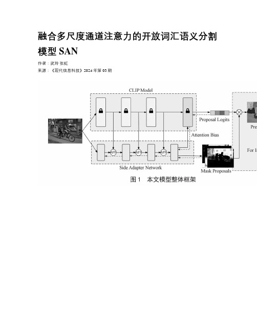
融合多尺度通道注意力的开放词汇语义分割模型SAN作者：武玲张虹来源：《现代信息科技》2024年第03期收稿日期：2023-11-29基金项目：太原师范学院研究生教育教学改革研究课题（SYYJSJG-2154）DOI：10.19850/ki.2096-4706.2024.03.035摘要：随着视觉语言模型的发展，开放词汇方法在识别带注释的标签空间之外的类别方面具有广泛应用。

相比于弱监督和零样本方法，开放词汇方法被证明更加通用和有效。

文章研究的目标是改进面向开放词汇分割的轻量化模型SAN，即引入基于多尺度通道注意力的特征融合机制AFF来改进该模型，并改进原始SAN结构中的双分支特征融合方法。

然后在多个语义分割基准上评估了该改进算法，结果显示在几乎不改变参数量的情况下，模型表现有所提升。

这一改进方案有助于简化未来开放词汇语义分割的研究。

关键词：开放词汇；语义分割；SAN；CLIP；多尺度通道注意力中图分类号：TP391.4；TP18 文献标识码：A 文章编号：2096-4706（2024）03-0164-06An Open Vocabulary Semantic Segmentation Model SAN Integrating Multi Scale Channel AttentionWU Ling， ZHANG Hong（Taiyuan Normal University， Jinzhong 030619， China）Abstract： With the development of visual language models， open vocabulary methods have been widely used in identifying categories outside the annotated label. Compared with the weakly supervised and zero sample method， the open vocabulary method is proved to be more versatile and effective. The goal of this study is to improve the lightweight model SAN for open vocabularysegmentation， which introduces a feature fusion mechanism AFF based on multi scale channel attention to improve the model， and improve the dual branch feature fusion method in the original SAN structure. Then， the improved algorithm is evaluated based on multiple semantic segmentation benchmarks， and the results show that the model performance has certain improvement with almost no change in the number of parameters. This improvement plan will help simplify future research on open vocabulary semantic segmentation.Keywords： open vocabulary; semantic segmentation; SAN; CLIP; multi scale channel attention 0 引言識别和分割任何类别的视觉元素是图像语义分割的追求。

语义分析的一些方法

语义分析的一些方法语义分析的一些方法(上篇)•5040语义分析，本文指运用各种机器学习方法，挖掘与学习文本、图片等的深层次概念。

wikipedia上的解释：In machine learning, semantic analysis of a corpus is the task of building structures that approximate concepts from a large set of documents(or images)。

工作这几年，陆陆续续实践过一些项目，有搜索广告，社交广告，微博广告，品牌广告，内容广告等。

要使我们广告平台效益最大化，首先需要理解用户，Context(将展示广告的上下文)和广告，才能将最合适的广告展示给用户。

而这其中，就离不开对用户，对上下文，对广告的语义分析，由此催生了一些子项目，例如文本语义分析，图片语义理解，语义索引，短串语义关联，用户广告语义匹配等。

接下来我将写一写我所认识的语义分析的一些方法，虽说我们在做的时候，效果导向居多，方法理论理解也许并不深入，不过权当个人知识点总结，有任何不当之处请指正，谢谢。

本文主要由以下四部分组成：文本基本处理，文本语义分析，图片语义分析，语义分析小结。

先讲述文本处理的基本方法，这构成了语义分析的基础。

接着分文本和图片两节讲述各自语义分析的一些方法，值得注意的是，虽说分为两节，但文本和图片在语义分析方法上有很多共通与关联。

最后我们简单介绍下语义分析在广点通“用户广告匹配”上的应用，并展望一下未来的语义分析方法。

1 文本基本处理在讲文本语义分析之前，我们先说下文本基本处理，因为它构成了语义分析的基础。

而文本处理有很多方面，考虑到本文主题，这里只介绍中文分词以及Term Weighting。

1.1 中文分词拿到一段文本后，通常情况下，首先要做分词。

分词的方法一般有如下几种：•基于字符串匹配的分词方法。

此方法按照不同的扫描方式，逐个查找词库进行分词。

综述Representation learning a review and new perspectives

explanatory factors for the observed input. A good representation is also one that is useful as input to a supervised predictor. Among the various ways of learning representations, this paper focuses on deep learning methods: those that are formed by the composition of multiple non-linear transformations, with the goal of yielding more abstract – and ultimately more useful – representations. Here we survey this rapidly developing area with special emphasis on recent progress. We consider some of the fundamental questions that have been driving research in this area. Speciﬁcally, what makes one representation better than another? Given an example, how should we compute its representation, i.e. perform feature extraction? Also, what are appropriate objectives for learning good representations?

隐语义模型常用的训练方法

隐语义模型常用的训练方法隐语义模型（Latent Semantic Model）是一种常用的文本表示方法，它可以将文本表示为一个低维的向量空间中的点，从而方便进行文本分类、聚类等任务。

在实际应用中，如何训练一个高效的隐语义模型是非常重要的。

本文将介绍隐语义模型常用的训练方法。

一、基于矩阵分解的训练方法1.1 SVD分解SVD（Singular Value Decomposition）分解是一种基于矩阵分解的方法，它可以将一个矩阵分解为三个矩阵相乘的形式，即A=UΣV^T。

其中U和V都是正交矩阵，Σ是对角线上元素为奇异值的对角矩阵。

在隐语义模型中，我们可以将用户-物品评分矩阵R分解为两个低维矩阵P和Q相乘的形式，即R≈PQ^T。

其中P表示用户向量矩阵，Q表示物品向量矩阵。

具体地，在SVD分解中，我们首先需要将评分矩阵R进行预处理。

一般来说，我们需要减去每个用户或每个物品评分的平均值，并对剩余部分进行归一化处理。

然后，我们可以使用SVD分解将处理后的评分矩阵R分解为P、Q和Σ三个矩阵。

其中，P和Q都是低维矩阵，Σ是对角线上元素为奇异值的对角矩阵。

通过调整P和Q的维度，我们可以控制模型的复杂度。

在训练过程中，我们需要使用梯度下降等方法来最小化预测评分与实际评分之间的误差。

具体地，在每次迭代中，我们可以随机选择一个用户-物品对（ui），计算预测评分pui，并根据实际评分rui更新P 和Q中相应向量的值。

具体地，更新公式如下：pu=pu+η(euiq-uλpu)qi=qi+η(euip-uλqi)其中η是学习率，λ是正则化参数，eui=rui-pui表示预测评分与实际评分之间的误差。

1.2 NMF分解NMF（Nonnegative Matrix Factorization）分解是另一种基于矩阵分解的方法，在隐语义模型中也有广泛应用。

与SVD不同的是，在NMF中要求所有矩阵元素都为非负数。

具体地，在NMF中，我们需要将评分矩阵R进行预处理，并将其分解为P和Q两个非负矩阵相乘的形式，即R≈PQ。

基于深度学习的多旋翼无人机单目视觉目标定位追踪方法

设计与应用・156・计算机测量与控制.2020. 28(4)Computer Measurement & Contrl文章编号：1671 - 4598(2020)04 - 0156 -05DOI ：10. 16526/j. cnki 11 — 4762/tp. 2020. 04. 032 中图分类号:V279 文献标识码：A基于深度学习的多旋翼无人机单目视觉目标定位追踪方法魏明鑫!黄浩!胡永明,王德志，李岳彬(湖北大学物理与电子科学学院&武汉 430062)摘要：针对无人机对目标的识别定位与跟踪&提出了一种基于深度学习的多旋翼无人机单目视觉目标识别跟踪方法&解决了传统的基于双目摄像机成本过高以及在复杂环境下识别准确率较低的问题；该方法基于深度学习卷积神经网络的目标检测算法&使用该算法对目标进行模型训练&将训练好的模型加载到搭载ROS 的机载电脑；机载电脑外接单目摄像机&单目摄像头检测目标后&自动检测出目标在图像中的位置&通过采用一种基于坐标求差的优化算法进行目标位置准确获取&然后将目标位置信息转化为控制无人机飞行的期望速度和高度发送给飞控板&飞控板接收到机载电脑发送的跟踪指令&实现对目标物体的跟踪；试验结果验证了该方法可以很好地进行目标识别并实现目标追踪％关键词：计算机视觉；深度学习；无人机；单目摄像机；目标跟踪Monocular Vision Target Tracking Method for Multi —rotorUnmanned Aerial Vehicle Based on Deep LearningWeiMingxin &Huang Hao &Hu Yongming &Wang Dezhi &Li Yuebin(Hubei Key Lab of Ferro — & Piezoelectric Materials and Devices, Faculty of Physics and Electronic Science,HubeiUniversity &Wuhan 430062&China )Abstract : Aiming at the target recognition , location and tracking of unmanned aerial vehicles (UAV ) , a multi —rotor UAV mo-nocularvisiontargetrecognitionandtracking methodbasedondeeplearningisproposed &whichsolvestheproblemsofhighcostoftraditionalbinocularcameraandlowrecognitionaccuracyincomplexenvironment Thismethodisbasedonthetargetdetectionalgo- rithmofdeeplearningconvolutionalneuralnetwork &whichisusedtoconducttargetmodeltrainingandloadthetrainedmodelintotheonboardcomputerequippedwith ROS Onboardcomputerexternalmonocularcamera &monocularcameradetectingtarget &theauto- matica l y detect the target in the image position &by adopting a kind of optimization algorithm based on coordinate for poor get target locationaccurate &thenthetargetpositioninformationintocontrolof UAV flight speed and heightexpectationforflightcontrol board &flightcontrolboardacceptingfo l owscommandssenttotheairbornecomputer &realizethetargetobjecttracking Experimen- talresultsshowthatthismethodcanrecognizeandtracktargetswe lKeywords ： computer vision ； deep learning ； unmanned aerial vehicles (UAV); monocular camera ； target trackingo 引言无人机(unmanned aerial vehicle, UAV) 主要分为旋翼无人机和固定翼无人机％多旋翼无人机是旋翼无人机的一种，具有灵活性好、稳定性强、可垂直起降等特点，比固定翼无人机机动性更强%因此&多旋翼无人机的应用场景更加广泛％随着多旋翼无人机技术近几年的发展，多旋翼无人机在民用和军用领域都有了很广的应用％民用上可以用在航拍、电力巡检、物流等领域；军事上更是可以用在军事侦察、目标打击等方面％收稿日期2019 -08 -19；修回日期2019 -08 -30.基金项目：湖北省自然科学基金指导性计划项目(2018CFC797) %作者简介：魏明鑫(1996 -"，男，湖北武汉人，硕士研究生，主要从事计算机视觉,机器人交互技术方向的研究％胡永明(1978 -)，男，江西资溪县人，博士，博士生导师，教授，主要从事光电传感器方向的研究％传统视觉跟踪虽然有很强的自主性、宽测量范围和可以获取大量的环境信息等优点，但它同时也存在许多缺点％&)强大的硬件系统是必需的：为了获得精确的导航信息，导航系统不可避免地配备了高分辨率相机和强大的处理器％从图像数据采集和处理，这涉及到巨大的数据操作%许多图像算法都是非常复杂的，这无疑给系统的集成设计、CPU 、DSP 、GPU 计算能力和内存大小带来了巨大的挑战％2)传统视觉导航跟踪的可靠性较差：视觉导航有时很难在复杂的灯光和温度变化的环境下工作％环境适应性问题是困扰视觉导航的难题%同时无法解决不同形状的物体在投影平面上的问题相同的图像视觉算法的高实时需求％所以视觉导航不仅需要高性能的硬件来提高图像采集的速度和处理时间，还需要在深度学习、神经网络和小波变换等软件算法上取得突破)16* %近几年，由于深度学习的发展，机器人无人驾驶等领第4期魏明鑫，等：基于深度学习的多旋翼无人机单目视觉目标定位追踪方法・157・域又迎来了一次变革&将朝着达到真正意义上的人工智能发展％目标跟踪无人机主要涉及视觉识别、目标检测与追踪等问题％文献介绍了一种基于合作目标的无人机目标跟踪方法％能够实现准确跟踪，此方法主要用在危险物排除％文献介绍了基于视觉的无人机目标追踪方法&该方法是采用数传将摄像机采集到的图像数据发送到远端进行处理后再发送指令给无人机％本文介绍一种基于深度学习的无人机目标跟踪方法&其自主性更强，解决了传统的基于双目摄像机成本过高以及在复杂环境下识别准确率较低的问题％通过深度学习SSD算法训练自己的模型&然后将训练好的模型移到嵌入式工控板并运行&使其能够辨认出要识别并且跟踪的目标%在嵌入式工控板中装的是Lnux操作系统&并在Lnux操作系统中安装了ROS(robot operating system)%ROS是一个用于编写机器人软件的灵活框架集成了大量的工具、库、协议&提供类似操作系统所提供的功能&可以极大简化繁杂多样的机器人平台下的复杂任务创建与稳定行为控制%因此嵌入式工控板可以通过ROS与飞控板建立通信％飞控板接收到目标物的位置并接受工控板发送的指令使无人机朝目标飞去&并实现追踪％系统分为三层&上层为视觉处理端&底层为飞控端&中间采用ROS作为通信机制％其系1基于深度学习的目标检测在计算机视觉领域&基于深度学习的目标检测算法近几年发展迅速&每年都有新的想法提出%R—CNN提出于2014年&是卷积神经网络在目标检测任务中的开山之作% R—CNN因为要对每个候选区都要从头开始计算整个网络&所以其运算效率低下%2015年RBG(RossB.Gishick)等结合了SPP—Net的共享卷积计算思想&对R—CNN做出改进&于是就有了FastR—CNN%RBG团队在2015年&与FastR—CNN同年推出了Faster R—CNN&Faster R—CNN的出现解决了Fast R—CNN的实时性问题，在Faster R—CNN中提到了RPN(Region Proposal Network)网络，RPN是一种全卷积网络&它的前几层卷积层和FasterR—CNN的前五层是一样的&所以RPN是在进一步的共享卷积层的计算&以降低区域建议的时间消耗％较大的提高了目标检测精度和计算速度卩10*%为了进一步提升目标检测的实时性&基于单个网络的实时目标检测框架YOLO(You Only Look Once)&框架和基于单个网络多层次预测框的目标检测算法SSD(Single Shoot MultiBox Detector)算法被提出%YOLO虽然能够达到实时的效果&但是其mAP与SSD的结果有很大的差距&每个网格只能预测一个目标&易导致漏检&对于目标的尺度较敏锐&对于尺度变化较大的目标泛化性较差⑴皿％而无人机目标检测对准确性要求更高％综合对比下来&本方案采用SSD目标检测算法%SSD的设计理念也是采用CNN网络来进行检测&不同的是&它采用了一个多尺度的特征图用来检测％多尺度检测顾名思义是采用尺寸不同的特征图&分别采用一个大的特征图和一个比较小的特征图用来检测％用大的特征图检测小的目标&小的特征图来检测大的目标％与YOLO采用的全连接层不同&SSD最后直接采用卷积对不同的特征图进行检测提取%SSD设置先验框&这里是借鉴了FasterR—CNN中anchor的思想%图2展示了其基本架构%图3展示了大小两个特征图的效果%图3不同尺寸的特征图SSD以VGG16为基础模型&在该模型上新增了卷积层来获取更多的特征图％从图4中&可以看到该算法利用了多尺度的特征图来做检测%・158・计算机测量与控制第28卷图4SSD算法网络结构图2目标追踪的原理目标识别出后并画框圈中目标物&开始进行目标追踪&目标追踪主要分为两步％目标位置估计以及控制无人机姿态进行追踪）2*%2.1目标位置坐标获取摄像头通过目标检测捕捉到目标&并画框提取％这里调用OpenCV处理方框&并将目标物所画方框的中心像素点坐标提取出来为P&（i&,y&）,相机画面中心像素点坐标为，2（化，y2）,接下来是获得深度距离信息&利用深度学习目标检测算法&被追踪目标可以有效并完整地框选出来&并计算选择框上下边距之间的像素尺寸％采用三角形相似原理）5*&计算得到目标上下框的尺寸&目标到摄像头间的距离满足：d=6（1）这里&d代表物体与摄像头之间的距离；=代表摄像头的焦距&这里所用的摄像头是定焦摄像头；h代表目标物体的实际长度；6代表目标成像后的长度&原理如图5所示％图5相似三角形距离估计原理示意图求得深度距离信息之后&我们就完整地得到了目标框中心像素点与相机画面中心像素点的三维坐标，然后计算相机画面中心像素与目标框中心像素在空间坐标系的坐标差&获取到无人机与目标物之间的坐标差&如图6所示％2.2PID算法控制无人机追踪将目标位置坐标差信息转换为控制无人机的期望速度%由于相机的抖动&系统输出的位置坐标存在误差&为了减小误差&我们这里采用了PID算法来优化输出的坐标差）6*%在基本PID控制中&当有较大幅度的扰动或大幅度改变给定值时&由于此时有较大的偏差&以及系统有惯性和滞后&故在积分项的作用下，往往会产生较大的超调量和长时间的波动％为此可以采用积分分离措施&即偏差较大时&取消积分作用&所以我们这里即用PD算法来改善系统的动态性能）6*%X oUT=K p:X e（）+"d:Y out=K p:y e）+"l:e y2x i e（）r e（—&（2"2y=y e（）—y^tt—i）这里，i et）&y et）为y轴的坐标差，，2y为系统误差％图7展示了经过优化后最终输出的目标位置％在机体坐标系下&前方z为正&右方r为正&下方y为正％flag—detected用作标志位，1代表识别到目标&0代表丢失目标%图7最终输出的目标位置示意图通过Mavlnk实时发布期望速度和高度给飞控&使飞控板对无人机进行姿态控制实现对目标的追踪％图8为无人机姿态控制的详细流程图％第4 期魏明鑫，等：基于深度学习的多旋翼无人机单目视觉目标定位追踪方法・159・目标识别画框像素中心坐标求距距取标及标获坐差目离位置PID控制位置反馈调节姿态反馈调节图8目标追踪控制流程图图9自制模型训练流程图B 试验结果及分析3.1硬件平台搭建试验采用自行搭建的无人机飞行平台进行&飞控板采用Pixhawk 同时外接工业级IMU ,使得无人机飞行时具有更好的稳定性，嵌入式工控板采用NVIDIA Jetson TX2 平台%3.2模型训练训练过程主要分为两个步骤：第一步是图片中的先验框与真实值进行匹配；第二步是确定损失函数％SSD 的先验框与真实值的匹配原则主要有两点：第一,对于图片中每个真实值&找到与其重叠度最大的先验框,然后该先验框与其进行匹配；第二&保证正负样本平衡, 保证正负样本的比例接近1 : 3%确定训练样本后&然后确定损失函数％损失函数是由位置误差和置信度误差加权和得到的&其公式为：L (X,c,l,g " = K (L conf (x ,c ) + aL Oc (X,l,g "" (3)式中& N 代表先验框的正样本的个数%这里x ) * {1, 0}代表一个指示参数&当x G = 1时表示第z 个先验框与第G 个真实值进行匹配%对于位置误差，其采用Smooth L1 Loss, 定义如下：NLi°c (x,l,g) 4Z* Pos m * {ex & cy &t & h }对于置信度误差，其采用SoftmaxLoss ,定义如下：L onf (X & c ) 4— —(5)这里：模型训练结束后&用训练好的模型检测效果％本文随机选取了几张坦克战车的照片&以此来检验模型对于坦克战车识别的准确率。

deep visual-semantic alignments for generating image descriptions

Deep Visual-Semantic Alignments for Generating Image DescriptionsAndrej Karpathy Li Fei-FeiDepartment of Computer Science,Stanford University{karpathy,feifeili}@AbstractWe present a model that generates free-form natural lan-guage descriptions of image regions.Our model leverages datasets of images and their sentence descriptions to learn about the inter-modal correspondences between text and vi-sual data.Our approach is based on a novel combination of Convolutional Neural Networks over image regions,bidi-rectional Recurrent Neural Networks over sentences,and a structured objective that aligns the two modalities through a multimodal embedding.We then describe a Recurrent Neu-ral Network architecture that uses the inferred alignments to learn to generate novel descriptions of image regions.We demonstrate the effectiveness of our alignment model with ranking experiments on Flickr8K,Flickr30K and COCO datasets,where we substantially improve on the state of the art.We then show that the sentences created by our gen-erative model outperform retrieval baselines on the three aforementioned datasets and a new dataset of region-level annotations.1.IntroductionA quick glance at an image is sufﬁcient for a human to point out and describe an immense amount of details about the vi-sual scene[8].However,this remarkable ability has proven to be an elusive task for our visual recognition models.The majority of previous work in visual recognition has focused on labeling images with aﬁxed set of visual categories,and great progress has been achieved in these endeavors[36,6]. However,while closed vocabularies of visual concepts con-stitute a convenient modeling assumption,they are vastly restrictive when compared to the enormous amount of rich descriptions that a human can compose.Some pioneering approaches that address the challenge of generating image descriptions have been developed[22,7]. However,these models often rely on hard-coded visual con-cepts and sentence templates,which imposes limits on their variety.Moreover,the focus of these works has been on re-ducing complex visual scenes into a single sentence,which we consider as an unnecessaryrestriction.Figure1.Our model generates free-form natural language descrip-tions of image regions.In this work,we strive to take a step towards the goal of generating dense,free-form descriptions of images(Figure1).The primary challenge towards this goal is in the de-sign of a model that is rich enough to reason simultaneously about contents of images and their representation in the do-main of natural language.Additionally,the model should be free of assumptions about speciﬁc hard-coded templates, rules or categories and instead rely primarily on training data.The second,practical challenge is that datasets of im-age captions are available in large quantities on the internet [14,46,29],but these descriptions multiplex mentions of several entities whose locations in the images are unknown.Our core insight is that we can leverage these large image-sentence datasets by treating the sentences as weak labels, in which contiguous segments of words correspond to some particular,but unknown location in the image.Our ap-proach is to infer these alignments and use them to learna generative model of descriptions.Concretely,our contri-butions are twofold:•We develop a deep neural network model that in-fers the latent alignment between segments of sen-1tences and the region of the image that they describe.Our model associates the two modalities through a common,multimodal embedding space and a struc-tured objective.We validate the effectiveness of this approach on image-sentence retrieval experiments in which we surpass the state-of-the-art.•We introduce a multimodal Recurrent Neural Network architecture that takes an input image and generates its description in text.Our experiments show that the generated sentences signiﬁcantly outperform retrieval-based baselines,and produce sensible qualitative pre-dictions.We then train the model on the inferred cor-respondences and evaluate its performance on a new dataset of region-level annotations.We make our code,data and annotations publicly available.2.Related WorkDense image annotations.Our work shares the high-level goal of densely annotating the contents of images with many works before us.Barnard et al.[1]and Socher et al.[38]studied the multimodal correspondence between words and images to annotate segments of images.Several works[26,12,9]studied the problem of holistic scene un-derstanding in which the scene type,objects and their spa-tial support in the image is inferred.However,the focus of these works is on correctly labeling scenes,objects and re-gions with aﬁxed set of categories,while our focus is on richer and higher-level descriptions of regions. Generating textual descriptions.Multiple works have ex-plored the goal of annotating images with textual descrip-tions on the scene level.A number of approaches pose the task as a retrieval problem,where the most compatible annotation in the training set is transferred to a test image [14,39,7,34,17],or where training annotations are broken up and stitched together[23,27,24].However,these meth-ods rely on a large amount of training data to capture the variety in possible outputs,and are often expensive at test time due to their non-parametric nature.Several approaches have been explored for generating image captions based on ﬁxed templates that areﬁlled based on the content of the im-age[13,22,7,43,44,4].This approach still imposes limits on the variety of outputs,but the advantage is that theﬁnal results are more likely to be syntactically correct.Instead of using aﬁxed template,some approaches that use a gen-erative grammar have also been developed[33,45].More closely related to our approach is the work of Srivastava et al.[40]who use a Deep Boltzmann Machine to learn a joint distribution over a images and tags.However,they do not generate extended phrases.More recently,Kiros et al.[19] developed a log-bilinear model that can generate full sen-tence descriptions.However,their model uses aﬁxed win-dow context,while our Recurrent Neural Network model can condition the probability distribution over the next word in the sentence on all previously generated words. Grounding natural language in images.A number of ap-proaches have been developed for grounding textual data in the visual domain.Kong et al.[20]develop a Markov Ran-dom Field that infers correspondences from parts of sen-tences to objects to improve visual scene parsing in RGBD images.Matuszek et al.[30]learn joint language and per-ception model for grounded attribute learning in a robotic setting.Zitnick et al.[48]reason about sentences and their grounding in cartoon scenes.Lin et al.[28]retrieve videos from a sentence description using an intermediate graph representation.The basic form of our model is in-spired by Frome et al.[10]who associate words and images through a semantic embedding.More closely related is the work of Karpathy et al.[18],who decompose images and sentences into fragments and infer their inter-modal align-ment using a ranking objective.In contrast to their model which is based on grounding dependency tree relations,our model aligns contiguous segments of sentences which are more meaningful,interpretable,and notﬁxed in length. Neural networks in visual and language domains.Mul-tiple approaches have been developed for representing im-ages and words in higher-level representations.On the im-age side,Convolutional Neural Networks(CNNs)[25,21] have recently emerged as a powerful class of models for image classiﬁcation and object detection[36].On the sen-tence side,our work takes advantage of pretrained word vectors[32,15,2]to obtain low-dimensional representa-tions of words.Finally,Recurrent Neural Networks have been previously used in language modeling[31,41],but we additionally condition these models on images.3.Our ModelOverview.The ultimate goal of our model is to generate descriptions of image regions.During training,the input to our model is a set of images and their corresponding sen-tence descriptions(Figure2).Weﬁrst present a model that aligns segments of sentences to the visual regions that they describe through a multimodal embedding.We then treat these correspondences as training data for our multimodal Recurrent Neural Network model which learns to generate the descriptions.3.1.Learning to align visual and language data Our alignment model assumes an input dataset of images and their sentence descriptions.The key challenge to in-ferring the association between visual and textual data is that sentences written by people make multiple references to some particular,but unknown locations in the image.For example,in Figure2,the words“Tabby cat is leaning”referFigure 2.Overview of our approach.A dataset of images and their sentence descriptions is the input to our model (left).Our model ﬁrst infers the correspondences (middle)and then learns to generate novel descriptions (right).to the cat,the words “wooden table”refer to the table,etc.We would like to infer these latent correspondences,with the goal of later learning to generate these snippets from image regions.We build on the basic approach of Karpa-thy et al.[18],who learn to ground dependency tree re-lations in sentences to image regions as part of a ranking objective.Our contribution is in the use of bidirectional recurrent neural network to compute word representations in the sentence,dispensing of the need to compute depen-dency trees and allowing unbounded interactions of words and their context in the sentence.We also substantially sim-plify their objective and show that both modiﬁcations im-prove ranking performance.We ﬁrst describe neural networks that map words and image regions into a common,multimodal embedding.Then we introduce our novel objective,which learns the embedding representations so that semantically similar concepts across the two modalities occupy nearby regions of the space.3.1.1Representing imagesFollowing prior work [22,18],we observe that sentencedescriptions make frequent references to objects and their attributes.Thus,we follow the method of Girshick et al.[11]to detect objects in every image with a Region Convo-lutional Neural Network (RCNN).The CNN is pre-trained on ImageNet [3]and ﬁnetuned on the 200classes of the ImageNet Detection Challenge [36].To establish fair com-parisons to Karpathy et al.[18],we use the top 19detected locations and the whole image and compute the represen-tations based on the pixels I b inside each bounding box as follows:v =W m [CNN θc (I b )]+b m ,(1)where CNN (I b )transforms the pixels inside bounding box I b into 4096-dimensional activations of the fully connected layer immediately before the classiﬁer.The CNN parame-ters θc contain approximately 60million parameters and the architecture closely follows the network of Krizhevsky et al [21].The matrix W m has dimensions h ×4096,where h is the size of the multimodal embedding space (h ranges from 1000-1600in our experiments).Every image is thus repre-sented as a set of h -dimensional vectors {v i |i =1...20}.3.1.2Representing sentencesTo establish the inter-modal relationships,we would like to represent the words in the sentence in the same h -dimensional embedding space that the image regions oc-cupy.The simplest approach might be to project every in-dividual word directly into this embedding.However,this approach does not consider any ordering and word context information in the sentence.An extension to this idea is to use word bigrams,or dependency tree relations as pre-viously proposed [18].However,this still imposes an ar-bitrary maximum size of the context window and requires the use of Dependency Tree Parsers that might be trained on unrelated text corpora.To address these concerns,we propose to use a bidirectional recurrent neural network (BRNN)[37]to compute the word representations.In our setting,the BRNN takes a sequence of N words (encoded in a 1-of-k representation)and trans-forms each one into an h -dimensional vector.However,the representation of each word is enriched by a variably-sized context around that ing the index t =1...N to denote the position of a word in a sentence,the precise form of the BRNN we use is as follows:x t =W w I t(2)e t =f (W e x t +b e )(3)h f t =f (e t +W f h ft −1+b f )(4)h b t =f (e t +W b h b t +1+b b )(5)s t =f (W d (h f t +h b t )+b d ).(6)Here,I t is an indicator column vector that is all zeros except for a single one at the index of the t -th word in a word vo-cabulary.The weights W w specify a word embedding ma-trix that we initialize with 300-dimensional word2vec [32]weights and keep ﬁxed in our experiments due to overﬁtting concerns.Note that the BRNN consists of two independent streams of processing,one moving left to right (h f t )and theother right to left (h bt )(see Figure 3for diagram).The ﬁ-nal h -dimensional representation s t for the t -th word is a function of both the word at that location and also its sur-rounding context in the sentence.Technically,every s t is a function of all words in the entire sentence,but our empir-Figure3.Diagram for evaluating the image-sentence score S kl. Object regions are embedded with a CNN(left).Words(enriched by their context)are embedded in the same multimodal space with a BRNN(right).Pairwise similarities are computed with inner products(magnitudes shown in grayscale)andﬁnally reduced to image-sentence score with Equation8.icalﬁnding is that theﬁnal word representations(s t)align most strongly to the visual concept of the word at that lo-cation(I t).Our hypothesis is that the strength of inﬂuence diminishes with each step of processing since s t is a more direct function of I t than of the other words in the sentence. We learn the parameters W e,W f,W b,W d and the respec-tive biases b e,b f,b b,b d.A typical size of the hidden rep-resentation in our experiments ranges between300-600di-mensions.We set the activation function f to the rectiﬁed linear unit(ReLU),which computes f:x→max(0,x).3.1.3Alignment objectiveWe have described the transformations that map every im-age and sentence into a set of vectors in a common h-dimensional space.Since our labels are at the level of en-tire images and sentences,our strategy is to formulate an image-sentence score as a function of the individual scores that measure how well a word aligns to a region of an im-age.Intuitively,a sentence-image pair should have a high matching score if its words have a conﬁdent support in the image.In Karpathy et al.[18],they interpreted the dot product v T i s t between an image fragment i and a sentence fragment t as a measure of similarity and used these to de-ﬁne the score between image k and sentence l as:S kl=t∈g li∈g kmax(0,v T i s t).(7)Here,g k is the set of image fragments in image k and g l is the set of sentence fragments in sentence l.The indices k,l range over the images and sentences in the training set. Together with their additional Multiple Instance Learning objective,this score carries the interpretation that a sentence fragment aligns to a subset of the image regions whenever the dot product is positive.We found that the following reformulation simpliﬁes the model and alleviates the need for additional objectives and their hyperparameters:S kl=t∈g lmax i∈gkv T i s t.(8)Here,every word s t aligns to the single best image region. As we show in the experiments,this simpliﬁed model also leads to improvements in theﬁnal ranking performance. Assuming that k=l denotes a corresponding image and sentence pair,theﬁnal max-margin,structured loss remains:C(θ)=klmax(0,S kl−S kk+1)rank images(9)+lmax(0,S lk−S kk+1)rank sentences.This objective encourages aligned image-sentences pairs to have a higher score than misaligned pairs,by a margin.3.1.4Decoding text segment alignments to images Consider an image from the training set and its correspond-ing sentence.We can interpret the quantity v T i s t as the un-normalized log probability of the t−th word describing any of the bounding boxes in the image.However,since we are ultimately interested in generating snippets of text instead of single words,we would like to align extended,contigu-ous sequences of words to a single bounding box.Note that the na¨ıve solution that assigns each word independently to the highest-scoring region is insufﬁcient because it leads to words getting scattered inconsistently to different regions. To address this issue,we treat the true alignments as latent variables in a Markov Random Field(MRF)where the bi-nary interactions between neighboring words encourage an alignment to the same region.Concretely,given a sentence with N words and an image with M bounding boxes,we introduce the latent alignment variables a j∈{1..M}for j=1...N and formulate an MRF in a chain structure along the sentence as follows:E(a)=j=1...NψU j(a j)+j=1...N−1ψB j(a j,a j+1)(10)ψU j(a j=t)=v T i s t(11)ψB j(a j,a j+1)=β1[a j=a j+1].(12) Here,βis a hyperparameter that controls the afﬁnity to-wards longer word phrases.This parameter allows us to interpolate between single-word alignments(β=0)andFigure4.Diagram of our multimodal Recurrent Neural Network generative model.The RNN takes an image,a word,the context from previous time steps and deﬁnes a distribution over the next word.START and END are special tokens.aligning the entire sentence to a single,maximally scoring region whenβis large.We minimize the energy toﬁnd the best alignments a using dynamic programming.The output of this process is a set of image regions annotated with seg-ments of text.We now describe an approach for generating novel phrases based on these correspondences.3.2.Multimodal Recurrent Neural Network forgenerating descriptionsIn this section we assume an input set of images and their textual descriptions.These could be full images and their sentence descriptions,or regions and text snippets as dis-cussed in previous sections.The key challenge is in the de-sign of a model that can predict a variable-sized sequence of outputs.In previously developed language models based on Recurrent Neural Networks(RNNs)[31,41,5],this is achieved by deﬁning a probability distribution of the next word in a sequence,given the current word and context from previous time steps.We explore a simple but effective ex-tension that additionally conditions the generative process on the content of an input image.More formally,the RNN takes the image pixels I and a sequence of input vectors (x1,...,x T).It then computes a sequence of hidden states (h1,...,h t)and a sequence of outputs(y1,...,y t)by iter-ating the following recurrence relation for t=1to T:b v=W hi[CNNθc(I)](13)h t=f(W hx x t+W hh h t−1+b h+b v)(14)y t=softmax(W oh h t+b o).(15) In the equations above,W hi,W hx,W hh,W oh and b h,b o are a set of learnable weights and biases.The output vector y t has the size of the word dictionary and one additional di-mension for a special END token that terminates the gener-ative process.Note that we provide the image context vector b v to the RNN at every iteration so that it does not have to remember the image content while generating words. RNN training.The RNN is trained to combine a word(x t), the previous context(h t−1)and the image information(b v) to predict the next word(y t).Concretely,the training pro-ceeds as follows(refer to Figure4):We set h0= 0,x1to a special START vector,and the desired label y1as theﬁrst word in the sequence.In particular,we use the word em-bedding for“the”as the START vector x1.Analogously, we set x2to the word vector of theﬁrst word and expect the network to predict the second word,etc.Finally,on the last step when x T represents the last word,the target label is set to a special END token.The cost function is to maximize the log probability assigned to the target labels.RNN at test time.The RNN predicts a sentence as follows: We compute the representation of the image b v,set h0=0, x1to the embedding of the word“the”,and compute the distribution over theﬁrst word y1.We sample from the dis-tribution(or pick the argmax),set its embedding vector as x2,and repeat this process until the END token is generated.3.3.OptimizationWe use Stochastic Gradient Descent with mini-batches of 100image-sentence pairs and momentum of0.9to optimize the alignment model.We cross-validate the learning rate and the weight decay.We also use dropout regularization in all layers except in the recurrent layers[47].The generative RNN is more difﬁcult to optimize,party due to the word frequency disparity between rare words,and very common words(such as the END token).We achieved the best re-sults using RMSprop[42],which is an adaptive step size method that scales the gradient of each weight by a running average of its gradient magnitudes.4.ExperimentsDatasets.We use the Flickr8K[14],Flickr30K[46]and COCO[29]datasets in our experiments.These datasets contain8,000,31,000and123,000images respectively and each is annotated with5sentences using Amazon Mechanical Turk.For Flickr8K and Flickr30K,we use 1,000images for validation,1,000for testing and the rest for training(consistent with[14,18]).For COCO we use 5,000images for both validation and testing.Data Preprocessing.We convert all sentences to lower-case,discard non-alphanumeric characters,andﬁlter out the articles“an”,“a”,and“the”for efﬁciency.Our word vocabulary contains20,000words.4.1.Image-Sentence Alignment EvaluationWeﬁrst investigate the quality of the inferred text and im-age alignments.As a proxy for this evaluation we perform ranking experiments where we consider a withheld set of images and sentences and then retrieve items in one modal-ity given a query from the other.We use the image-sentence score S kl(Section3.1.3)to evaluate a compatibility score between all pairs of test images and sentences.We then re-port the median rank of the closest ground truth result in theImage Annotation Image SearchModel R@1R@5R@10Med r R@1R@5R@10Med rDeViSE(Frome et al.[10]) 4.518.129.226 6.721.932.725SDT-RNN(Socher et al.[39])9.629.841.1168.929.841.116DeFrag(Karpathy et al.[18])12.632.944.0149.729.642.515Our implementation of DeFrag[18]13.835.848.210.49.528.240.315.6Our model:DepTree edges14.837.950.09.411.631.443.813.2Our model:BRNN16.540.654.27.611.832.144.712.4Flickr30KDeViSE(Frome et al.[10]) 4.518.129.226 6.721.932.725SDT-RNN(Socher et al.[39])9.629.841.1168.929.841.116DeFrag(Karpathy et al.[18])14.237.751.31010.230.844.214Our implementation of DeFrag[18]19.244.558.0 6.012.935.447.510.8Our model:DepTree edges20.046.659.4 5.415.036.548.210.4Our model:BRNN22.248.261.4 4.815.237.750.59.2COCOOur model:1K test images29.462.075.9 2.520.952.869.2 4.0Our model:5K test images11.832.545.412.28.924.936.319.5Table1.Image-Sentence ranking experiment results.R@K is Recall@K(high is good).Med r is the median rank(low is good).In the results for our models,we take the top5validation set models,evaluate each independently on the test set and then report the average performance.The standard deviations on the recall values range from approximately0.5to1.0.list and Recall@K,which measures the fraction of times a correct item was found among the top K results.The results of these experiments can be found in Table1,and exam-ple retrievals in Figure5.We now highlight some of the takeaways.Our full model outperforms previous work.We compare our full model(“Our model:BRNN”)to the following base-lines:DeViSE[10]is a model that learns a score between words and images.As the simplest extension to the setting of multiple image regions and multiple words,Karpathy et al.[18]averaged the word and image region representa-tions to obtain a single vector for each modality.Socher et al.[39]is trained with a similar objective,but instead of averaging the word representations,they merge word vec-tors into a single sentence vector with a Recursive Neural Network.DeFrag are the results reported by Karpathy et al.[18].Since we use different word vectors,dropout for regularization and different cross-validation ranges(includ-ing larger embedding sizes),we re-implemented their cost function for a fair comparison(“Our implementation of De-Frag”).In all of these cases,our full model(“Our model: BRNN”)provides consistent improvements.Our simpler cost function improves performance.We now try to understand the sources of these improvements. First,we removed the BRNN and used dependency tree re-lations exactly as described in Karpathy et al.[18](“Our model:DepTree edges”).The only difference between this model and“Our reimplementation of DeFrag”is the new, simpler cost function introduced in Section3.1.3.We see that our formulation shows consistent improvements.BRNN outperforms dependency tree relations.Further-more,when we replace the dependency tree relations with the BRNN,we observe additional performance improve-ments.Since the dependency relations were shown to work better than single words and bigrams[18],this suggests that the BRNN is taking advantage of contexts longer than two words.Furthermore,our method does not rely on extracting a Dependency Tree and instead uses the raw words directly. COCO results for future comparisons.The COCO dataset has only recently been released,and we are not aware of other published ranking results.Therefore,we re-port results on a subset of1,000images and the full set of 5,000test images for future comparisons.Qualitative.As can be seen from example groundings in Figure5,the model discovers interpretable visual-semantic correspondences,even for small or relatively rare objects such as“seagulls”and“accordion”.These details would be missed by models that only reason about full images. 4.2.Evaluation of Generated DescriptionsWe have demonstrated that our alignment model produces state of the art ranking results and qualitative experiments suggest that the model effectively infers the alignment be-tween words and image regions.Our task is now to synthe-size these sentence snippets given new image regions.We evaluate these predictions with the BLEU[35]score,which despite multiple problems[14,22]is still considered to be the standard metric of evaluation in this setting.The BLEU score evaluates a candidate sentence by measuring the frac-tion of n-grams that appear in a set of references.Figure5.Example alignments predicted by our model.For every test image above,we retrieve the most compatible test sentence and visualize the highest-scoring region for each word(before MRF smoothing described in Section3.1.4)and the associated scores(v T i s t). We hide the alignments of low-scoring words to reduce clutter.We assign each region an arbitrary color.Flickr8K Flickr30K COCOMethod of generating text B-1B-2B-3B-1B-2B-3B-1B-2B-3Human agreement0.590.350.160.640.360.160.570.310.13Ranking:Nearest Neighbor0.290.110.030.270.080.020.320.110.03Generating:RNN0.420.190.060.450.200.060.500.250.12Table2.BLEU score evaluation of full image predictions on1,000images.B-n is BLEU score that uses up to n-grams(high is good).Our multimodal RNN outperforms retrieval baseline. Weﬁrst verify that our multimodal RNN is rich enough to support sentence generation for full images.In this experi-ment,we trained the RNN to generate sentences on full im-ages from Flickr8K,Flickr30K,and COCO datasets.Then at test time,we use theﬁrst four out ofﬁve sentences as references and theﬁfth one to evaluate human agreement. We also compare to a ranking baseline which uses the best model from the previous section(Section4.1)to annotate each test image with the highest-scoring sentence from the training set.The quantitative results of this experiment are in Table2.Note that the RNN model conﬁdently outper-forms the retrieval method.This result is especially interest-ing in COCO dataset,since its training set consists of more than600,000sentences that cover a large variety of de-scriptions.Additionally,compared to the retrieval baseline which compares each image to all sentences in the training set,the RNN takes a fraction of a second to evaluate.We show example fullframe predictions in Figure6.Our generative model(shown in blue)produces sensible de-scriptions,even in the last two images that we consider to be failure cases.Additionally,we veriﬁed that none of these sentences appear in the training set.This suggests that the model is not simply memorizing the training data.How-ever,there are20occurrences of“man in black shirt”and 60occurrences of“is paying guitar”,which the model may have composed to describe theﬁrst image.Region-level evaluation.Finally,we evaluate our region RNN which was trained on the inferred,intermodal corre-spondences.To support this evaluation,we collected a new dataset of region-level annotations.Concretely,we asked8 people to label a subset of COCO test images with region-level text descriptions.The labeling interface consisted of a single test image,and the ability to draw a bounding box and annotate it with text.We provided minimal constraints and instructions,except to“describe the content of each box”and we encouraged the annotators to describe a large variety of objects,actions,stuff,and high-level concepts. Theﬁnal dataset consists of1469annotations in237im-ages.There are on average6.2annotations per image,and each one is on average4.13words long.We compare three models on this dataset:The region RNN model,a fullframe RNN model that was trained on full im-ages and sentences,and a ranking baseline.To predict de-scriptions with the ranking baseline,we take the number of words in the shortest reference annotation and search the training set sentences for the highest scoring segment of text。

1、下载文档前请自行甄别文档内容的完整性，平台不提供额外的编辑、内容补充、找答案等附加服务。
2、"仅部分预览"的文档,不可在线预览部分如存在完整性等问题,可反馈申请退款(可完整预览的文档不适用该条件!)。
3、如文档侵犯您的权益，请联系客服反馈,我们会尽快为您处理(人工客服工作时间：9:00-18:30)。

___________________________________________________________________
Focus on movement data has increased as a consequence of the larger availability of such data due to current GPS, GSM, RFID, and sensors techniques. In parallel, interest in movement has shifted from raw movement data analysis to more application-oriented ways of analyzing segments of movement suitable for the specific purposes of the application. This trend has promoted semantically rich trajectories, rather than raw movement, as the core object of interest in mobility studies. This survey provides the definitions of the basic concepts about mobility data, an analysis of the issues in mobility data management, and a survey of the approaches and techniques for i) constructing trajectories from movement tracks, ii) enriching trajectories with semantic information to enable the desired interpretations of movements, and iii) using data mining to analyze semantic trajectories and extract knowledge about their characteristics, in particular the behavioral patterns of the moving objects. Last but not least, the paper surveys the new privacy issues that rise due to the semantic aspects of trajectories. Categories and Subject Descriptors: H. Information Systems, H.2. Database Management, H.2.0 General General Terms: algorithms, design, legal aspects, management Additional Key Words and Phrases: movement, mobility tracks, tracking, mobility data, trajectories, trajectory behavior, semantic enrichment, data mining, activity identification, GPS
________________________________________________________________________
This work is supported by the EU, FET OPEN, 2009-2012 Programme, Coordination Action type Project MODAP (Mobility, Data Mining, and Privacy) Authors’ addresses: Gennady and Natalia Andrienko, Fraunhofer Institute IAIS, Schloss Birlinghoven, Sankt-Augustin, D53754 Germany, email: {gennady|natalia}.andrienko@iais.fraunhofer.de; Vania Bogorny, UFSC-CTC-INE, CEP 88040-900 - Campus Universitário Cx.P. 476, Florianópolis S.C., Brazil, vania@inf.ufsc.br; Maria Luisa Damiani: Università degi Studi di Milano, Via Comelico 39, 20135 Milano, Italy, email: mdamiani@dico.unimi.it; Aris Gkoulalas-Divanis: IBM Research GmbHschlikon, Switzerland, agd@; José Macedo: Campus do PICI, Computer Science Department, Fortaleza, Brazil, CEP 60.115-190, jose.macedo@lia.ufc.br; Christine Parent: Université de Lausanne HEC-ISI, 1015 Lausanne, Switzerland, email: christine.parent@unil.ch; Nikos Pelekis: Department of Statistics and Insurance Science, University of Piraeus, Karaoli-Dimitriou 80, Piraeus, GR-18534, Greece, email: npelekis@unipi.gr; Chiara Renso: ISTI–CNR, Via Moruzzi 1, 56010, Pisa, Italy, email: chiara.renso@r.it; Stefano Spaccapietra and Zhixian Yan: EPFL-IC-LSIR, Station 14, CH-1015 Lausanne, email: {stefano.spaccapietra, zhixian.yan}@epfl.ch; Yannis Théodoridis: Department of Informatics, University of Piraeus, GR-18534 Piraeus, Greece, email: ytheod@unipi.gr
1.
INTRODUCTION1
Mobility is one of the major keywords that characterize the current development of our society. People, goods and ideas are moving faster and more frequently than ever. Ubiquitous computing facilities and location-based services have greatly supported human mobility. More recently, GPS and other positioning devices enabled capturing the evolving position of objects moving in geographical space. Massive amounts of tracking data have been created, for the benefit of novel applications that build on this movement knowledge. Researchers from the database, GIS, visualization, data mining, and knowledge extraction communities have developed models and techniques for mobility analysis. Their results represent an important step forward over previous foundational work done by e.g. Güting et al. on moving objects [Güting et al. 2000], and the EU Chorochronos project [Koubarakis et al. 2003] on spatio-temporal data. A detailed survey of mobility research up to 2007 has been published in [Giannotti and Pedreschi 2008] as part of the EU GeoPKDD project (www.geopkdd.eu). Over the last few years the corpus of mobility techniques has greatly expanded. In particular, a new promising approach has been devised to provide applications with richer and more meaningful knowledge about movement. This is achieved by combining the raw mobility tracks (e.g. the GPS records) with related contextual data. These enriched track records are referred to as semantic trajectories. This paper surveys the new ideas and techniques related to the elaboration and analysis of semantic trajectories. Some of the ideas and techniques previously developed for raw trajectories will nevertheless be mentioned for better understandability. An extensive coverage of previous techniques can be found in [Zheng and Zhou 2011]. Our paper is purposely focused on data mining techniques, as these are the most frequently used in the literature. Other techniques (e.g. visual analytics [Andrienko et al. 2011], and aggregation techniques) also play an important role in movement analysis, but they would require a full survey on their own to be properly discussed. The sequel of the paper is organized as follows. Sections 2 and 3 define the basic concepts and terminology that support our analysis of trajectories and their behaviors. Next we discuss the three steps to convert raw data into knowledge: Trajectory reconstruction (Section 4), semantic enrichment (Section 5) and behavior knowledge extraction (Section 6). Section 7 surveys the privacy issues that characterize human trajectories. The conclusion introduces foreseeable future developments.