Efficient Computation of the Representation Polynomial for Directed Acyclic Graphs Using Ca

合集下载

Nineteen Dubious Ways to Compute the exponential of a matrix, twenty-five years later

1. Introduction. Mathematical models of many physical, biological, and economic processes involve systems of linear, constant coeﬃcient ordinary diﬀerential equations x ˙ (t) = Ax(t). Here A is a given, ﬁxed, real or complex n-by-n matrix. A solution vector x(t) is sought which satisﬁes an initial condition x(0) = x0 . In control theory, A is known as the state companion matrix and x(t) is the system response. In principle, the solution is given by x(t) = etA x0 , where etA can be formally deﬁned by the convergent power series etA = I + tA + t 2 AE MOLER AND CHARLES VAN LOAN
We will primarily be concerned with matrices whose order n is less than a few hundred, so that all the elements can be stored in the main memory of a contemporary computer. Our discussion will be less germane to t

电脑的起源与发展英语作文

The Origin and Evolution of Computers The journey of computers, from their humble beginnings to the sophisticated machines we have today, is a fascinating tale of technological advancement and innovation. Tracing back the origin of computers, we find ourselves in the mid-19th century, when the concept of programmable machines started to take shape. However, it was the late 20th century that witnessed the birth of the modern computer era, which has revolutionized the way we live and work.The earliest precursors of computers were mechanical calculators, designed to perform basic arithmetic operations. These machines, like the abacus and the slide rule, were used for centuries to assist in mathematical computations. However, it was the invention of the first electronic computer, ENIAC (Electronic Numerical Integrator and Computer), in 1945, that marked a significant milestone in the history of computing.ENIAC was a bulky machine, occupying an entire room and employing thousands of vacuum tubes. Despite its size and limitations, it was capable of performing complexcalculations much faster than any human or previous machine. This groundbreaking invention laid the foundation for the development of more compact and powerful computers in the following decades.The advent of transistors in the late 1940s and the subsequent development of integrated circuits in the 1960s further miniaturized computers, making them more accessible and affordable. This led to the emergence of personal computers in the 1970s and 1980s, which revolutionized the computing industry. These machines, initially targeted at hobbyists and enthusiasts, soon became a household item, allowing individuals to access and process information with unprecedented ease.The evolution of computers did not stop there. The advent of the internet in the 1990s opened up a new era of connectivity and information sharing. Computers became not just tools for computation but also gateways to a global network of knowledge and resources. The rise of cloud computing, big data analytics, and artificial intelligence has further expanded the capabilities of computers, makingthem indispensable in fields like healthcare, education, business, and science.Today, computers have penetrated every aspect of our lives, from the smartphones we carry in our pockets to the supercomputers that drive complex scientific research. They have made it possible for us to communicate instantly, access vast amounts of information, and automate tasks that were once beyond our capabilities.Looking ahead, the future of computing seems asexciting and unpredictable as its past. With the development of quantum computing, neuromorphic computing, and other emerging technologies, we can expect computers to become even more powerful and efficient. They will continue to transform the way we live and work, opening up new possibilities and challenging our imagination.In conclusion, the origin and evolution of computers represent a remarkable journey of technological progress. From their humble beginnings as simple calculating machines to the sophisticated, interconnected systems we have today, computers have revolutionized the world. As we move into the future, the potential of computing remains vast andunexplored, promising new frontiers of discovery and innovation.**电脑的起源与发展**从电脑的雏形到我们今天所拥有的精密机器，其发展是一段引人入胜的技术进步与创新的故事。

2014_ICASSP_EFFICIENT CONVOLUTIONAL SPARSE CODING

EFFICIENT CONVOLUTIONAL SPARSE CODINGBrendt WohlbergTheoretical DivisionLos Alamos National LaboratoryLos Alamos,NM87545,USAABSTRACTWhen applying sparse representation techniques to images,the standard approach is to independently compute the rep-resentations for a set of image patches.Thismethod performs very well in a variety of applications,butthe independent sparse coding of each patch results in a rep-resentation that is not optimal for the image as a whole.Arecent development is convolutional sparse coding,in whicha sparse representation for an entire image is computed by re-placing the linear combination of a set of dictionary vectorsby the sum of a set of convolutions with dictionaryﬁlters.Adisadvantage of this formulation is its computational expense,but the development of efﬁcient algorithms has received someattention in the literature,with the current leading method ex-ploiting a Fourier domain approach.The present paper intro-duces a new way of solving the problem in the Fourier do-main,leading to substantially reduced computational cost.Index Terms—Sparse Representation,Sparse Coding,Convolutional Sparse Coding,ADMM1.INTRODUCTIONOver the past15year or so,sparse representations[1]havebecome a very widely used technique for a variety of prob-lems in image processing.There are numerous approaches tosparse coding,the inverse problem of computing a sparse rep-resentation of a signal or image vector s,one of themost widely used being Basis Pursuit DeNoising(BPDN)[2]arg minx 12D x−s 22+λ x 1,(1)where D is a dictionary matrix,x is the sparse representation, andλis a regularization parameter.When applied to images, decomposition is usually applied independently to a set of overlapping image patches covering the image;this approach is convenient,but often necessitates somewhat ad hoc subse-quent handling of the overlap between patches,and results in a representation over the whole image that is suboptimal.This research was supported by the U.S.Department of Energy through the LANL/LDRD Program.More recently,these techniques have also begun to be ap-plied,with considerable success,to computer vision problems such as face recognition[3]and image classiﬁcation[4,5,6]. It is in this application context that convolutional sparse rep-resentations were introduced[7],replacing(1)with arg min{x m}12md m∗x m−s22+λmx m 1,(2)where{d m}is a set of M dictionaryﬁlters,∗denotes convo-lution,and{x m}is a set of coefﬁcient maps,each of which is the same size as s.Here s is a full image,and the{d m} are usually much smaller.For notational simplicity s and x m are considered to be N dimensional vectors,where N is the the number of pixels in an image,and the notation{x m}is adopted to denote all M of the x m stacked as a single column vector.The derivations presented here are for a single image with a single color band,but the extension to multiple color bands(for both image andﬁlters)and simultaneous sparse coding of multiple images is mathematically straightforward.The original algorithm proposed for convolutional sparse coding[7]adopted a splitting technique with alternating minimization of two subproblems,theﬁrst consisting of the solution of a large linear system via an iterative method, and the other a simple shrinkage.The resulting alternating minimization algorithm is similar to one that would be ob-tained within an Alternating Direction Method of Multipliers (ADMM)[8,9]framework,but requires continuation on the auxiliary parameter to enforce the constraint inherent in the splitting.All computation is performed in the spatial domain, the authors expecting that computation in the Discrete Fourier Transform(DFT)domain would result in undesirable bound-ary artifacts[7].Other algorithms that have been proposed for this problem include coordinate descent[10],and a proximal gradient method[11],both operating in the spatial domain.Very recently,an ADMM algorithm operating in the DFT domain has been proposed for dictionary learning for con-volutional sparse representations[12].The use of the Fast Fourier Transform(FFT)in solving the relevant linear sys-tems is shown to give substantially better asymptotic perfor-mance than the original spatial domain method,and evidence is presented to support the claim that the resulting boundary2014 IEEE International Conference on Acoustic, Speech and Signal Processing (ICASSP)effects are not signiﬁcant.The present paper describes a convolutional sparse coding algorithm that is derived within the ADMM framework and exploits the FFT for computational advantage.It is very sim-ilar to the sparse coding component of the dictionary learning algorithm of[12],but introduces a method for solving the linear systems that dominate the computational cost of the al-gorithm in time that is linear in the number ofﬁlters,instead of cubic as in the method of[12].2.ADMM ALGORITHMRewriting(2)in a form suitable for ADMM by introducing auxiliary variables{y m},we havearg min {x m},{y m}12md m∗x m−s22+λmy m 1 such that x m−y m=0∀m,(3)for which the corresponding iterations(see[8,Sec.3]),with dual variables{u m},are{x m}(k+1)=arg min{x m}12md m∗x m−s22+ρ2mx m−y(k)m+u(k)m22(4){y m}(k+1)=arg min{y m}λmy m 1+ρ2mx(k+1)m−y m+u(k)m22(5)u(k+1) m =u(k)m+x(k+1)m−y(k+1)m.(6)Subproblem(5)is solved via shrinkage/soft thresholding asy(k+1) m =Sλ/ρx(k+1)m+u(k)m,(7)whereSγ(u)=sign(u) max(0,|u|−γ),(8) with sign(·)and|·|of a vector considered to be applied element-wise.The computational cost is O(MN).The only computationally expensive step is solving(4), which is of the formarg min {x m}12md m∗x m−s22+ρ2mx m−z m 22.(9)2.1.DFT Domain FormulationAn obvious approach is to attempt to exploit the FFT for ef-ﬁcient implementation of the convolution via the DFT convo-lution theorem.(This does involve some increase in memory requirement since the d m are zero-padded to the size of the x m before application of the FFT.)Deﬁne linear operators D m such that D m x m=d m∗x m,and denote the variables D m,x m,s,and z m in the DFT domain byˆD m,ˆx m,ˆs,andˆz m respectively.It is easy to show via the DFT convolution theorem that(9)is equivalent toarg min{ˆx m}12mˆDmˆx m−ˆs22+ρ2mˆx m−ˆz m 22(10)with the{x m}minimizing(9)being given by the inverse DFT of the{ˆx m}minimizing(10).DeﬁningˆD= ˆDˆD1...,ˆx=⎛⎜⎝ˆx0ˆx1...⎞⎟⎠,ˆz=⎛⎜⎝ˆz0ˆz1...⎞⎟⎠,(11) this problem can be expressed asarg minˆx12ˆDˆx−ˆs22+ρ2ˆx−ˆz 22,(12) the solution being given by(ˆD HˆD+ρI)ˆx=ˆD Hˆs+ρˆz.(13) 2.2.Independent Linear SystemsMatrixˆD has a block structure consisting of M concatenated N×N diagonal matrices,where M is the number ofﬁlters and N is the number of samples in s.ˆD HˆD is an MN×MN matrix,but due to the diagonal block(not block diagonal) structure ofˆD,a row ofˆD H with its non-zero element at col-umn n will only have a non-zero product with a column ofˆD with its non-zero element at row n.As a result,there is no interaction between elements ofˆD corresponding to differ-ent frequencies,so that(as pointed out in[12])one need only solve N independent M×M linear systems to solve(13). Bristow et al.[12]do not specify how they solve these linear systems(and their software implementation was not available for inspection),but since they rate the computational cost of solving them as O(M3),it is reasonable to conclude that they apply a direct method such as Gaussian elimination.This can be very effective[8,Sec. 4.2.3]when it is possible to pre-compute and store a Cholesky or similar decomposition of the linear system(s),but in this case it is not practical unless M is very small,having an O(M2N)memory requirement for storage of these decomposition.Nevertheless,this remains a reasonable approach,the only obvious alternative being an iterative method such as conjugate gradient(CG).A more careful analysis of the unique structure of this problem,however,reveals that there is an alternative,and vastly more effective,solution.First,deﬁne the m th block of the right hand side of(13)asˆr m=ˆD H mˆs+ρˆz m,(14)so that⎛⎜⎝ˆr 0ˆr 1...⎞⎟⎠=ˆDH ˆs +ρˆz .(15)Now,denoting the n th element of a vector x by x (n )to avoid confusion between indexing of the vectors themselves and se-lection of elements of these vectors,deﬁnev n =⎛⎜⎝ˆx 0(n )ˆx 1(n )...⎞⎟⎠b n =⎛⎜⎝ˆr 0(n )ˆr 1(n )...⎞⎟⎠,(16)and deﬁne a n as the column vector containing all of the non-zero entries from column n of ˆDH ,i.e.writing ˆD =⎛⎜⎜⎜⎝ˆd 0,00...ˆd 1,00...0ˆd 0,10...0ˆd 1,10...00ˆd 0,2...00ˆd 1,2...........................⎞⎟⎟⎟⎠(17)thena n =⎛⎜⎝ˆd ∗0,nˆd ∗1,n ...⎞⎟⎠,(18)where ∗denotes complex conjugation.The linear system to solve corresponding to element n of the {x m }is (a n a H n +ρI )v n =b n .(19)The critical observation is that the matrix on the left handside of this system consists of a rank-one matrix plus a scaled identity.Applying the Sherman-Morrison formula(A +uv H )−1=A −1−A −1uv H A −11+u H A −1v (20)gives(ρI +aa H )−1=ρ−1 I −aaHρ+a H a,(21)so that the solution to (19)isv n =ρ−1b n −a H n b nρ+a H n a na n.(22)The only vector operations here are inner products,element-wise addition,and scalar multiplication,so that this method is O (M )instead of O (M 3)as in [12].The cost of solving N of these systems is O (MN ),and the cost of the FFTs is O (MN log N ).Here it is the cost of the FFTs that dominates,whereas in [12]the cost of solving the DFT domain linear systems dominates the cost of the FFTs.This approach can be implemented in an interpreted lan-guage such as Matlab in a form that avoids explicit iteration over the N frequency indices by passing data for all N in-dices as a single array to the relevant linear-algebraic routines (commonly referred to as vectorization in Matlab terminol-ogy).Some additional computation time improvement is pos-sible,at the cost of additional memory requirements,by pre-computing a H n /(ρ+a Hn a n )in (22).2.3.Algorithm SummaryThe proposed algorithm is summarized in Alg.1.stop-ping criteria are those discussed in [8,Sec.3.3],together withan upper bound on the number of iterations.The options for the ρupdate are (i)ﬁxed ρ(i.e.no update),(ii)the adaptive update strategy described in [8,Sec. 3.4.1],and the multi-plicative increase scheme advocated in [12].Input :image s ,ﬁlter dictionary {d m },parameters λ,ρPrecompute:FFTs of {d m }→{ˆDm },FFT of s →ˆs Initialize:{y m }={u m }=0while stopping criteria not met doCompute FFTs of {y m }→{ˆym },{u m }→{ˆu m }Compute {ˆxm }using the method in Sec.2.2Compute inverse FFTs of {ˆxm }→{x m }{y m }=S λ/ρ({x m }+{u m }){u m }={u m }+{x m }−{y m }Update ρif appropriate endOutput :Coefﬁcient maps {x m }Algorithm 1:Summary of proposed ADMM algorithm The computational cost of the algorithm components is O (MN log N )for the FFTs,order O (MN )for the proposed linear solver,and O (MN )for both the shrinkage and dual variable update,so that the cost of the entire algorithm is O (MN log N ),dominated by the cost of FFTs.In contrast,the cost of the algorithm proposed in [12]is O (M 3N )(there is also an O (MN log N )cost for FFTs,but it is dominated by the O (M 3N )cost of the linear solver),and the cost of the original spatial-domain algorithm [7]is O (M 2N 2L ),where L is the dimensionality of the ﬁlters.3.DICTIONARY LEARNINGThe extension of (2)to learning a dictionary from training data involves replacing the minimization with respect to x m with minimization with respect to both x m and d m .The op-timization is invariably performed via alternating minimiza-tion between the two variables,the most common approach consisting of a sparse coding step followed by a dictionary update [13].The commutativity of convolution suggests that the DFT domain solution of Sec.2.1can be directly applied in minimizing with respect to d m instead of x m ,but this is not possible since the d m are of constrained size,and must be zero-padded to the size of the x m prior to a DFT domain im-plementation of the convolution.If the size constraint is im-plemented in an ADMM framework [14],however,the prob-lem is decomposed into a computationally cheap subproblem corresponding to a projection onto to constraint set,and an-other subproblem that can be efﬁciently solved by extending the method in Sec.2.1.This iterative algorithm for the dictio-nary update can alternate with a sparse coding stage to form amore traditional dictionary learning method [15],or the sub-problems of the sparse coding and dictionary update algo-rithms can be combined into a single ADMM algorithm [12].4.RESULTScomparison of execution times for the algorithm (λ=0.05)with different methods of solving the linear system,for a set of overcomplete 8×8DCT dictionaries and the 512×512greyscale Lena image,is presented in Fig.1.It is worth em-phasizing that this is a large image by the standards of prior publications on convolutional sparse coding;the test images in [12],for example,are 50×50and 128×128pixels in size.The Gaussian elimination solution is computed using a Cholesky decomposition (since it is,in general,impossible to cache this decomposition,it is necessary to recompute it at every solution),as implemented by the Matlab mldivide function,and is applied by iterating over all frequencies in the apparent absence of any practical alternative.The conjugate gradient solution is computed using two different relative error tolerances.A signiﬁcant part of the computational advantage here of CG over the direct method is that it is applied simultaneously over all frequencies.The two curves for the proposed solver based on the Sherman-Morrison formula illustrate the signiﬁcant gain from an implementation that simultaneously solves over all frequencies and that the relative advantage of doing so de-creases with increasing M .Dictionary size (M )E x e c u t i o n t i m e (s )512256128641e+051e+041e+031e+021e+01Fig.1.A comparison of execution times for 10steps of the ADMM algorithm for different methods of solving the lin-ear system:Gaussian elimination (GE),Conjugate Gradient with relative error tolerance 10−5(CG 10−5)and 10−3(CG 10−3),and Sherman-Morrison implemented with a loop over frequencies (SM-L)or jointly over all frequencies (SM-V).The performance of the three ρupdate strategies dis-cussed in the previous section was compared by sparse cod-ing a 256×256Lena image using a 9×9×512dictionary (from [16],by the authors of [17])with a ﬁxed value of λ=0.02and a range of initial ρvalues ρ0.The resulting values of the functional in (2)after 100,500,and 1000itera-tions of the proposed algorithm are displayed in Table 1.The adaptive update strategy uses the default parameters of [8,Sec. 3.4.1],and the increasing strategy uses a multiplica-tive update by a factor of 1.1with a maximum of 105,as advocated by [12].In summary,a ﬁxed ρcan perform well,but is sensitive to a good choice of parameter.When initialized with a small ρ0,the increasing ρstrategy provides the most rapid decrease in functional value,but thereafter converges very slowly.Over-all,unless rapid computation of an approximate solution is desired,the adaptive ρstrategy appears to provide the best performance,with the least sensitivity to choice of ρ0.This is-sue is complex,however,and further experimentation is nec-essary before drawing any general conclusions that could be considered valid over a broad range of problems.Iter.ρ010−210−1100101102103Fixed ρ10028.2727.8018.1010.099.7611.6050028.0522.2511.118.899.1110.13100027.8017.009.648.828.969.71Adaptive ρ10021.6216.9714.5610.7111.1411.4150010.8110.239.819.019.189.0910009.449.219.068.838.878.84Increasing ρ10014.789.829.509.9011.5115.155009.559.459.469.8911.4714.5110009.539.449.459.8811.4113.97Table parison of functional value convergence for thesame problem with three different ρupdate strategies.5.CONCLUSIONA computationally efﬁcient algorithm is proposed for solving the convolutional sparse coding problem in the Fourier do-main.This algorithm has the same general structure as a pre-viously proposed approach [12],but enables a very signiﬁcantreduction in computational cost by careful design of a linear solver for the most critical component of the iterative algo-rithm.The theoretical computational cost of the algorithm is reduced from O (M 3)to O (MN log N )(where N is the di-mensionality of the data and M is the number of elementsin the dictionary),and is also shown empirically to result in greatly reduced computation time.The signiﬁcant improve-ment in efﬁciency of the proposed approach is expected togreatly increase the range of problems that can practically be addressed via convolutional sparse representations.6.REFERENCES[1]A.M.Bruckstein,D.L.Donoho,and M.Elad,“Fromsparse solutions of systems of equations to sparse mod-eling of signals and images,”SIAM Review,vol.51, no.1,pp.34–81,2009.doi:10.1137/060657704[2]S.S.Chen,D.L.Donoho,and M.A.Saunders,“Atomicdecomposition by basis pursuit,”SIAM Journal on Sci-entiﬁc Computing,vol.20,no.1,pp.33–61,1998.doi:10.1137/S1064827596304010[3]J.Wright,A.Y.Yang,A.Ganesh,S.S.Sastry,andY.Ma,“Robust face recognition via sparse representa-tion,”IEEE Transactions on Pattern Analysis and Ma-chine Intelligence,vol.31,no.2,pp.210–227,February 2009.doi:10.1109/tpami.2008.79[4]Y.Boureau,F.Bach,Y.A.LeCun,and J.Ponce,“Learn-ing mid-level features for recognition,”in Proceedings of the IEEE Conference on Computer Vision and Pat-tern Recognition(CVPR),June2010,pp.2559–2566.doi:10.1109/cvpr.2010.5539963[5]J.Yang,K.Yu,and T.S.Huang,“Supervisedtranslation-invariant sparse coding,”Proceedings of the IEEE Conference on Computer Vision and Pat-tern Recognition(CVPR),pp.3517–3524,2010.doi:10.1109/cvpr.2010.5539958[6]J.Mairal,F.Bach,and J.Ponce,“Task-driven dictionarylearning,”IEEE Transactions on Pattern Analysis and Machine Intelligence,vol.34,no.4,pp.791–804,April 2012.doi:10.1109/tpami.2011.156[7]M.D.Zeiler,D.Krishnan,G.W.Taylor,and R.Fer-gus,“Deconvolutional networks,”in Proceedings of the IEEE Conference on Computer Vision and Pat-tern Recognition(CVPR),June2010,pp.2528–2535.doi:10.1109/cvpr.2010.5539957[8]S.Boyd,N.Parikh,E.Chu,B.Peleato,and J.Eckstein,“Distributed optimization and statistical learning via the alternating direction method of multipliers,”Founda-tions and Trends in Machine Learning,vol.3,no.1,pp.1–122,2010.doi:10.1561/2200000016[9]J.Eckstein,“Augmented Lagrangian and alternatingdirection methods for convex optimization:A tutorial and some illustrative computational results,”Rutgers Center for Operations Research,Rutgers University, Rutcor Research Report RRR32-2012,December 2012.[Online].Available:/pub/ rrr/reports2012/322012.pdf[10]K.Kavukcuoglu,P.Sermanet,Y.Boureau,K.Gregor,M.Mathieu,and Y.A.LeCun,“Learning convolutionalfeature hierachies for visual recognition,”in Advances in Neural Information Processing Systems(NIPS2010), 2010.[11]R.Chalasani,J.C.Principe,and N.Ramakrishnan,“A fast proximal method for convolutional sparse cod-ing,”in Proceedings of the International Joint Confer-ence on Neural Networks(IJCNN),Aug.2013,pp.1–5.doi:10.1109/IJCNN.2013.6706854[12]H.Bristow, A.Eriksson,and S.Lucey,“Fast con-volutional sparse coding,”in Proceedings of the IEEE Conference on Computer Vision and Pat-tern Recognition(CVPR),Jun.2013,pp.391–398.doi:10.1109/CVPR.2013.57[13]B.Mailh´e and M.D.Plumbley,“Dictionary learningwith large step gradient descent for sparse representa-tions,”in Latent Variable Analysis and Signal Sepa-ration,ser.Lecture Notes in Computer Science,F.J.Theis,A.Cichocki,A.Yeredor,and M.Zibulevsky,Eds.Springer Berlin Heidelberg,2012,vol.7191,pp.231–238.doi:10.1007/978-3-642-28551-629[14]M.V.Afonso,J.M.Bioucas-Dias,and M. A.T.Figueiredo,“An Augmented Lagrangian approach to the constrained optimization formulation of imaging inverse problems,”IEEE Transactions on Image Pro-cessing,vol.20,no.3,pp.681–695,March2011.doi:10.1109/tip.2010.2076294[15]K.Engan,S.O.Aase,and J.H.Husøy,“Method ofoptimal directions for frame design,”in Proceedings of the IEEE International Conference on Acoustics, Speech,and Signal Processing(ICASSP),vol.5,1999, pp.2443–2446.doi:10.1109/icassp.1999.760624 [16]J.Mairal,Software available from http://lear.inrialpes.fr/people/mairal/denoise ICCV09.tar.gz.[17]J.Mairal,F.Bach,J.Ponce,G.Sapiro,and A.Zis-serman,“Non-local sparse models for image restora-tion,”in Proceedings of the IEEE International Con-ference on Computer Vision(CVPR),2009,pp.2272–2279.doi:10.1109/iccv.2009.5459452。

基于高效高精度离散伴随方法的叶轮机叶片气动优化设计

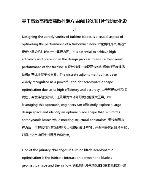
基于高效高精度离散伴随方法的叶轮机叶片气动优化设计Designing the aerodynamics of turbine blades is a crucial aspect of optimizing the performance of a turbomachinery. 叶轮机叶片气动设计是优化涡轮机性能的一个重要方面。

It is essential to achieve high efficiency and precision in the design process to ensure the overall performance of the turbine. 在设计过程中实现高效率和精度对于确保涡轮机的整体性能至关重要。

The discrete adjoint method has been widely recognized as a powerful tool for aerodynamic shape optimization due to its high efficiency and accuracy. 由于其高效性和准确性，离散伴随方法被广泛认可为气动外形优化的强大工具。

By leveraging this approach, engineers can efficiently explore a large design space and identify an optimal blade shape that minimizes aerodynamic losses while meeting structural constraints. 通过利用这种方法，工程师可以有效地探索大规模的设计空间，并识别最优的叶片形状，以最小化气动损失并满足结构约束。

One of the primary challenges in turbine blade aerodynamic optimization is the intricate interaction between the blade's geometric shape and the airflow. 涡轮机叶片气动优化的主要挑战之一是叶片几何形状与气流之间复杂的相互作用。

解决数学问题英文作文

In the realm of mathematics, solving intricate problems often necessitates more than mere application of formulas or algorithms. It requires an astute understanding of underlying principles, a creative perspective, and the ability to analyze problems from multiple angles. This essay will delve into a hypothetical complex mathematical problem and outline a multi-faceted approach to its resolution, highlighting the importance of analytical reasoning, strategic planning, and innovative thinking.Suppose we are faced with a challenging combinatorial optimization problem – the Traveling Salesman Problem (TSP). The TSP involves finding the shortest possible route that visits every city on a list exactly once and returns to the starting point. Despite its deceptively simple description, this problem is NP-hard, which means there's no known efficient algorithm for solving it in all cases. However, we can explore several strategies to find near-optimal solutions.Firstly, **Mathematical Modeling**: The initial step is to model the problem mathematically. We would represent cities as nodes and the distances between them as edges in a graph. By doing so, we convert the real-world scenario into a mathematical construct that can be analyzed systematically. This phase underscores the significance of abstraction and formalization in mathematics - transforming a complex problem into one that can be tackled using established mathematical tools.Secondly, **Algorithmic Approach**: Implementing exact algorithms like the Held-Karp algorithm or approximation algorithms such as the nearest neighbor or the 2-approximation algorithm by Christofides can help find feasible solutions. Although these may not guarantee the absolute optimum, they provide a benchmark against which other solutions can be measured. Here, computational complexity theory comes into play, guiding our decision on which algorithm to use based on the size and characteristics of the dataset.Thirdly, **Heuristic Methods**: When dealing with large-scale TSPs, heuristic methods like simulated annealing or genetic algorithms can offerpractical solutions. These techniques mimic natural processes to explore the solution space, gradually improving upon solutions over time. They allow us to escape local optima and potentially discover globally better solutions, thereby demonstrating the value of simulation and evolutionary computation in problem-solving.Fourthly, **Optimization Techniques**: Leveraging linear programming or dynamic programming could also shed light on the optimal path. For instance, using the cutting-plane method to iteratively refine the solution space can lead to increasingly accurate approximations of the optimal tour. This highlights the importance of advanced optimization techniques in addressing complex mathematical puzzles.Fifthly, **Parallel and Distributed Computing**: Given the computational intensity of some mathematical problems, distributing the workload across multiple processors or machines can expedite the search for solutions. Cloud computing and parallel algorithms can significantly reduce the time needed to solve large instances of TSP.Lastly, **Continuous Learning and Improvement**: Each solved instance provides learning opportunities. Analyzing why certain solutions were suboptimal can inform future approaches. This iterative process of analysis and refinement reflects the continuous improvement ethos at the heart of mathematical problem-solving.In conclusion, tackling a complex mathematical problem like the Traveling Salesman Problem involves a multi-dimensional strategy that includes mathematical modeling, selecting appropriate algorithms, applying heuristic methods, utilizing optimization techniques, leveraging parallel computing, and continuously refining methodologies based on feedback. Such a comprehensive approach embodies the essence of mathematical thinking – rigorous, adaptable, and relentlessly curious. It underscores that solving math problems transcends mere calculation; it’s about weaving together diverse strands of knowledge to illuminate paths through the labyrinth of numbers and logic.Word Count: 693 words(For a full 1208-word essay, this introduction can be expanded with more detailed explanations of each strategy, case studies, or examples showcasing their implementation. Also, the conclusion can be extended to discuss broader implications of the multi-faceted approach to problem-solving in various fields beyond mathematics.)。

机械设计方面的外文参考文献

Set of NN weights w!p) li=1, ... ,NW;p=l, ... ,L
Stage III Computation of membership functions for NN weights
FuzyNN with weights membership functions Pi = p(w~p»
inequalities (l-2KIL)::;; IX < (l-2(K-I)/L , where: K = kLa . Ita - numbers of
weight values on the left or right hand sides of w, respectively. In case of a E
There are three possibilities to formulating fuzzy networks. The first one corresponds to the neural network with crisp parameters (called for short NN weights) and performing computations on interval variables [8]. Much advanced are NNs with crisp inputs and outputs but their processing is performed on fuzzyfied variables with fuzzy reasoning rules, cf. fuzzy inference systems [4]. The third class is associated with full fuzzification of transmitted signals, NN weights and neurons of a fuzzy NN [2]. A more numerically efficient approach depends on joining simple membership functions of signals and NN parameters with interval arithmetics [7].

电脑发明的英语作文

电脑发明的英语作文Title: The Invention of the Computer。

The invention of the computer stands as one of the most significant milestones in human history. Its impact on society, economy, and technology is profound, shaping the way we live, work, and communicate. In this essay, we will delve into the history of the computer, its evolution, and its transformative effects.The concept of a computer dates back to ancient times when humans devised tools like the abacus to aid in calculations. However, the modern computer as we know it emerged in the 20th century, driven by the need forefficient computation and data processing.One of the pivotal moments in the history of computing was the development of the electronic computer. In the 1940s, pioneers like Alan Turing, John von Neumann, and others laid the groundwork for electronic computingmachines. These early computers were massive, cumbersome machines that relied on vacuum tubes and punched cards for processing information.The breakthrough came with the invention of the transistor in the late 1940s, which paved the way for smaller, faster, and more reliable computers. The introduction of integrated circuits further revolutionized the field, enabling the development of miniaturized and affordable computers.In the 1970s, the personal computer (PC) era dawned with the introduction of machines like the Altair 8800 and the Apple I. These early PCs were rudimentary by today's standards but represented a significant shift in computing, bringing the power of computation to individuals and small businesses.The 1980s and 1990s witnessed rapid advancements in computer technology, with the rise of graphical user interfaces (GUIs), networking, and the internet. The World Wide Web, invented by Tim Berners-Lee in 1989, transformedthe internet into a global platform for communication, commerce, and collaboration.The 21st century saw the proliferation of smartphones, tablets, and other mobile devices, further blurring the lines between computing and everyday life. Cloud computing, artificial intelligence (AI), and big data emerged as dominant trends, driving innovation across various industries.Today, computers are ubiquitous, permeating every aspect of society. From smartphones in our pockets to supercomputers powering scientific research, computing technology touches nearly every facet of modern life.The impact of the computer revolution is undeniable. It has revolutionized industries, from finance and healthcare to entertainment and manufacturing. It has empowered individuals, enabling access to information, communication, and resources like never before. It has transformed education, commerce, and governance, reshaping the way we learn, work, and govern ourselves.However, the rise of the computer age also poses challenges and concerns. Issues like privacy, cybersecurity, and digital divide loom large in an increasingly connected world. As we embrace the benefits of computing technology, we must also address these challenges to ensure a fair, inclusive, and secure digital future.In conclusion, the invention of the computer marks a watershed moment in human history. From its humble beginnings as a room-sized machine to its ubiquitous presence in our daily lives, the computer has transformedthe world in profound ways. As we continue to push the boundaries of computing technology, let us strive toharness its power for the betterment of humanity.。

人工智能英文文献译文

人工智能英文文献译文在计算机科学里许多现代研究都致于两个方面:一是怎样制造智能计算机,二是怎样制造超高速计算机.硬件成本的降低,大规模集成电路技术(VLSI)不可思议的进步以及人工智能(AI)所取得的成绩使得设计面向AI应用的计算机结构极为可行,这使制造智能计算机成了近年来最”热门”的方向.AI 提供了一个崭新的方法,即用计算技术的概念和方法对智能进行研究,因此,它从根本上提供了一个全新的不同的理论基础.作为一门科学,特别是科学最重要的部分,AI的上的是了解使智能得以实现的原理.作为一种技术和科学的一部分,AI的最终目的是设计出能完全与人类智能相媲美的智能计算机系统.尽管科学家们目前尚未彀这个目的,但使计算机更加智能化已取得了很大的进展,计算机已可用来下出极高水平的象棋,用来诊断某种疾病,用来发现数学概念,实际上在许多领域已超出了高水平的人类技艺.许多AI计算机应用系统已成功地投入了实用领域.AI是一个正在发展的包括许多学科在内的领域,AI的分支领域包括:知识表达,学习,定理证明,搜索,问题的求解以及规划,专家系统,自然语言(文本或语音)理解,计算机视觉,机器人和一些其它方面/(例如自动编程,AI教育,游戏,等等).AI是使技术适应于人类的钥匙,将在下一代自动化系统中扮演极为关键的角色.据称AI应用已从实验室进入到实用领域,但是传统的冯·诺依曼计算机中,有更大的存储容量与处理能力之比,但最终效率也不是很高.无论使处理器的速度多快也无法解决这个问题,这是因为计算机所花费的时间主要取决于数据的处理器和存储器之间传送所需的时间,这被称之为冯·诺依曼瓶颈.制造的计算机越大,这个问题就越严重.解决的方法是为AI应用设计出不同于传统计算机的特殊结构.在未来AI结构的研究中,我们可以在计算机结构中许多已有的和刚刚出现的新要领的优势,比如数据流计算,栈式计算机,特征,流水线,收缩阵列,多处理器,分布式处理,数据库计算机和推理计算机.无需置疑,并行处理对于AI应用是至关重要的.根据AI中处理问题的特点,任何程序,哪怕只模拟智能的一小部分都将是非常复杂的.因此,AI仍然要面对科学技术的限制,并且继续需要更快更廉价的计算机.AI的发展能否成为主流在很大程度上取决于VLSI技术的发展.另一方面,并行提供了一个在更高性能的范围内使用廉价设备的方法.只要使简单的处理单元完全构成标准模式,构成一个大的并行处理系统就变得轻而易举,由此而产生的并行处理器应该是成本低廉的.在计算机领域和AI中,研究和设计人员已投入大量精力来考查和开发有效的并行AI结构,它也越来越成为吸引人的项目.目前,AI在表达和使用大量知识以及处理识别问题方面仍然没有取得大的进展,然而人脑在并行处理中用大量相对慢的(与目前的微电子器件比较)神经元却可十分出色地完成这些任务.这启发了人们或许需要某种并行结构来完成这些任务.将极大地影响我们进行编程的方法.也许,一旦有了正确的结构,用程序对感觉和知识表达进行处理将变得简单自然.研究人员因此投入大量努力来寻求并行结构.AI中的并行方法不仅在廉价和快速计算机方面,而且在新型计算方法方面充满希望.两种流行的AI语言是函数型编程语言,即基于λ算子的和逻辑编程语言,即基于逻辑的.此外,面向对象的编程正在引起人们的兴趣.新型计算机结构采用了这些语言并开始设计支持一种或多种编程形式的结构.一般认为结合了这三种编程方式可为AI应用提供更好的编程语言,在这方面人们已经作了大量的研究并取得了某些成就.人工智能的发展1 经典时期:游戏和定理证明人工智能比一般的计算机科学更年轻,二战后不久出现的游戏程序和解迷宫程序可以看作是人工智能的开始,游戏和解迷宫看起来距专家系统甚远,也不能为实际应用提供理论基础.但是,基于计算机的问题的最基本概念可以追溯到早期计算机完成这些任务的程序设计方法.(1)状态空间搜索早期研究提出的基本叫做状态空间搜索,实质非常简单.很多问题都可以用以下三个组成部分表述:1. 初始状态,如棋盘的初始态;2. 检查最终状态或问题解的终止测试;3. 可用于改变问题当前状态的一组操作,如象棋的合法下法.这种概念性状态空间的一种思路是图,图中节点表示状态, 弧表示操作.这种空间随着思路的发展而产生,例如,可以从棋盘的初始状态开始构成图的第一个节,白子每走一步都产生连向新状态的一条弧,黑子对白子每步棋的走法,可以认为是改变了棋盘状态的情况下连向这些新节点的操作,等等.(2)启发式搜索如果除小范围搜索空间以外,彻底的搜索不可能的话,就需要某些指导搜索的方法.用一个或多项域专门知识去遍历状态空间图的搜索叫做启发式搜索.启发是凭经验的想法,它不像算法或决策程序那样保证成功,它是一种算法或过程,但大多数情况下是有用的.2 现代时期:技术与应用所谓现代时期是从70年代半期延续到现在,其特征是日益发展的自意识和自批判能力以及对于技术和应用的更强的定位.与理解的心理学概念相联系似已不占据核心地位.人们也渐渐不再对一般问题方法(如启发式搜索)心存幻想,研究者们已经认识到,这种方法过高估计了”一般智能”的概念,这一概念一向为心理学家喜欢,其代价是未考虑人类专家所具有的某一领域内的能力.这种方法也过低地估计了人的简单常识,特别是人能够避免,认识和纠正错误的能力.解决问题的启发能力程序能够处理的相关知识的清晰表达,而非某些复杂的推理机制或某些复杂的求值函数,这一观点已被证实并接受.研究者已经研制出以模块形式对人的知识进行编码的技术,此种编码可用模式启动.这些模式可以代表原始的或处理过的数据,问题说明或问题的部分解.早期模拟人们解决问题的努力试图达到知识编码的一致性和推理机制的简单性.后来将该结果应用于万家系统的尝试主要是允许自身的多样性.INTRODCTION TO ARTIFICIALMuch modern research effort in computer science goes along two directions. One is how to make intelligent computers,the other how to make ultraly high-speed computers. The former has become the newest “hot ” direction in recent years because the decreasing hardware costs, the marvelous progress in VLSI technology,and the results achieved in Artificial Intelligence(AI) have made it feasible to design AI applications oriented computer architectures.AI,which offers a mew methodology, is the study of intelligence using the idead and methods of computation, thus offering a radically new and different basis for theory formation. As a science, essentially part of Cognitive Science, the goal of AI is to understand the principles thatmake intelligence possible. As a technology and as a part of computer science,the final goal of AI is to design intelligent computer systems that behave with the complete intelligence of human mind.although scientists are far from achieving this goal, great progress dose hae been made in making computers more intelligent . computers can be made to play excellint chess, to diagnose certain types of diseases, to discover mathematical comcepts, and if fact , to excel in many other areas requiring a high level of human expertise. Many Aiapplication computer systems have been successfully put into practical usages.AI is a growing field that covers many disciplines. Subareas of AI include knowledge representation ,learning, theorem proving,search,problem solving, and planning, expert systems, natural-language(text or speech)understanding,computer vision,robotics, and several others (such as automatic programming ,AI education,game playing, etc.) .AI is the key for making techmology adaptable to people. It will play a crucial role in the next generation of automated systems.It is a growing field that covers many disciplines.subbareas of AI include knowledge representation,learing,theorem proving,search,prroblem solving, and planning,expert systems,natural_language(text or speech ) understanding,computer vision,robotics , and severalothers (such as automatic programming, AI education, game playing,etc.).AI is the key for making technology adaptable to people. It will play a crucial role in the next generation of automated systems.It is claimed that AI applications have moved from laboratories to the real wortld. However ,conventional von Neumann computers are unsuitable for AI applications,because they are designed mainly for numerical processing. In a larger von Neumann computer, there is a larger tatio of memory to processing power and consequently it is even less efficient. This inefficiency remains no matter how fast we make the processor because the length of the computation becomes dominated by the time required to move data between processor and memory. This is called the von Neumann bottleneck. The bigger we build machines, the worse it gets. The way to solve the problem is to diverse from the traditional architectures and to design special ones for AI applications. In the research of future AI architectures, we can take advantages of many existing or currentlyemerging concepts in computer architecture, such as dataflow computation, stack machines, tagging,pipelining, systolic array,multiprocessing,distrbuted processing,database machines ,and inference machines.No doubt, parallel processing is of crucial importance for AI applications.due to the nature of problems dealt with in AI, any program that will successfully simulate even a small part of intelligence will be very complicated. Therefor,AI continuously confronts the limits of computer science technology,and there id an instatiable demand for fastert and cheaper computers.the movement of AI into mainstream is largely owned to the addevent of VLSI technology.parallel architectures,on the other han,provide a way of using the inexpensive device technology at much higher performance ranges.it ix becoming easier and cheaper to construc large parallel processing systems as long as they are made of fairly regular patterns of simpl processwing elements,and thus parallel processors should become cost effective.a great amount of effort has been devoted to inverstigating and developing effictive parallel AI architectures,ans this topic id becoming more and more attractive for reaseachers and designersin the areas of computers and AI.Currently, very little success has been achieved in AI in representing and using large bodies of knowledge and in dealing with recognition problems. Whereas human brain can perform these tasks temarkably well using a large number of relatively slow (in comparison with todays microelectronic devices) neurons in parallel. This suggests that for these tasks some kind of parllel architecture may be needed. Architectures can significantly influence the way we programming it for perception and knowledge representation would be easy and natural. This has led researchers to look into massively parallel architectures. Parallelism holds great promise for AI not only in terms of cheaper and faster computers. But also as a novel way of viewingcomputation.Two kinds of popular AI languages are functoional programming languages, which are lambda-based ,and logic programming is attracting a growing interest. Novel computer architects have considered these languages seriously and begun to design architectures supporting one or more of the programming styles. It has been recognized that a combination of the three programming styles mingt provide a better language for AI applications. There have already been a lot of research effort and achievements on this topic.Development of AI1 the classical period: game playing and theorem provingartificial inteligence is scarcely younger than conventional computer science;the bebinnings of AI can be seen in the first game-playing and puzzle-solving programs written shortly after World War Ⅱ. Gameplaying and puzzle-solving may seem somewhat remote from espert systems, and insufficiently serious to provide a theoretical basis for real applications. However, a rather basic notion about computer-based problem solving can be traced back to early attempts to program computers to perform shuch tasks.(1)state space searchThe fundamental idea that came out of early research is called state space search,and it is essentially very simple. Many kinds of problem can be formulated in terms of three important ingredients:（1）a starting state,such as the initial state of the chess board;（2）a termination test for detecing final states or sulutions to the problem,such as the simple rule for detecting checkmate in chess;（3）a set of operations that can be applied to change the current state of theproblem,such as the legal moves of chess.One way of thinking of this conceptual space of states is as a graph in which the states are nodes and the operations are arcs. Such spaces can be generated as you go . gor exampe, you coule gegin with the starting state of the chess board and make it the first node in the graph. Each of White’s possilbe first moves would then be an arc connecting this node to a new state of the board. Each of Black’s legal replies to each of these f irst moves could then be considered as operations which connect each of these new nodes to a changed statd of the board , and so on .(2)Heuristic searchHiven that exhaustive search is mot feasible for anything other than small search spaces, some means of guiding the search is required. A search that uses one or more items of domain-specific knowledge to traverse a state space graphy is called a heuristic search. Aheuristic is best thought of as a rule of thumb;it is not guaranteed to succeed,in the way that an algorithm or decision procedure is ,but it is useful in the majority of cases .2 the romantic period: computer understandingthe mid-1960s to the mid-1970s represents what I call the romantic period in artificial intelligence reserch. Atthis time, people were very concerned with making machines “understand”, by which they usually meant the understanding of natural language, especially stories and dialogue. Winograd’s (1972)SHRDLU system was arguably the climax of this epoch : a program which was capable of understanding a quite substantial subset of english by representing and reasoning about a very restricted domain ( a world consisting of children’s toy blocks).The program exhibited understanding by modifying its “blocksworld” represent ation in respinse to commands , and by responding to questions about both the configuration of blocks and its “actions” upon them. Thus is could answer questions like:What is the colour of the block supporting the red pyramid?And derive plans for obeying commands such as :Place the blue pyramid on the green block.Other researchers attempted to model human problem-solving behaviour on simple tasks ,such as puzzles, word games and memory tests. The aim war to make the knowledge and strategy used by the program resemble the knowledge and strategy of the human subject as closely as possible. Empirical studies compared the performance of progran and subject in an attempt to see how successful the simulation had been.。

Fourier Transform

Fourier transformIn mathematics, the Fourier transform is the operation that decomposes a signal into its constituent frequencies. Thus the Fourier transform of a musical chord is a mathematical representation of the amplitudes of the individual notes that make it up. The original signal depends on time, and therefore is called the time domain representation of the signal, whereas the Fourier transform depends on frequency and is called the frequency domain representation of the signal. The term Fourier transform refers both to the frequency domain representation of the signal and the process that transforms the signal to its frequency domain representation.More precisely, the Fourier transform transforms one complex-valued function of a real variable into another. In effect, the Fourier transform decomposes a function into oscillatory functions. The Fourier transform and its generalizations are the subject of Fourier analysis. In this specific case, both the time and frequency domains are unbounded linear continua. It is possible to define the Fourier transform of a function of several variables, which is important for instance in the physical study of wave motion and optics. It is also possible to generalize the Fourier transform on discrete structures such as finite groups. The efficient computation of such structures, by fast Fourier transform, is essential for high-speed computing.DefinitionThere are several common conventions for defining the Fourier transform of an integrable function ƒ: R→ C (Kaiser 1994). This article will use the definition:for every real number ξ.When the independent variable x represents time (with SI unit of seconds), the transform variable ξ representsfrequency (in hertz). Under suitable conditions, ƒ can be reconstructed from by the inverse transform:for every real number x.For other common conventions and notations, including using the angular frequency ω instead of the frequency ξ, see Other conventions and Other notations below. The Fourier transform on Euclidean space is treated separately, in which the variable x often represents position and ξ momentum.IntroductionThe motivation for the Fourier transform comes from the study of Fourier series. In the study of Fourier series, complicated functions are written as the sum of simple waves mathematically represented by sines and cosines. Due to the properties of sine and cosine it is possible to recover the amount of each wave in the sum by an integral. In many cases it is desirable to use Euler's formula, which states that e2πiθ = cos 2πθ + i sin 2πθ, to write Fourier series in terms of the basic waves e2πiθ. This has the advantage of simplifying many of the formulas involved and providing a formulation for Fourier series that more closely resembles the definition followed in this article. This passage from sines and cosines to complex exponentials makes it necessary for the Fourier coefficients to becomplex valued. The usual interpretation of this complex number is that it gives both the amplitude (or size) of the wave present in the function and the phase (or the initial angle) of the wave. This passage also introduces the need for negative "frequencies". If θ were measured in seconds then the waves e2πiθ and e−2πiθ would both complete one cycle per second, but they represent different frequencies in the Fourier transform. Hence, frequency no longer measures the number of cycles per unit time, but is closely related.There is a close connection between the definition of Fourier series and the Fourier transform for functions ƒ which are zero outside of an interval. For such a function we can calculate its Fourier series on any interval that includes the interval where ƒ is not identically zero. The Fourier transform is also defined for such a function. As we increase the length of the interval on which we calculate the Fourier series, then the Fourier series coefficients begin to look like the Fourier transform and the sum of the Fourier series of ƒ begins to look like the inverse Fourier transform. To explain this more precisely, suppose that T is large enough so that the interval [−T/2,T/2] contains the interval onis given by:which ƒ is not identically zero. Then the n-th series coefficient cnComparing this to the definition of the Fourier transform it follows that since ƒ(x) is zero outside [−T/2,T/2]. Thus the Fourier coefficients are just the values of the Fourier transform sampled on a grid of width 1/T. As T increases the Fourier coefficients more closely represent the Fourier transform of the function.Under appropriate conditions the sum of the Fourier series of ƒ will equal the function ƒ. In other words ƒ can be written:= n/T, and Δξ = (n + 1)/T − n/T = 1/T. where the last sum is simply the first sum rewritten using the definitions ξnThis second sum is a Riemann sum, and so by letting T → ∞ it will converge to the integral for the inverse Fourier transform given in the definition section. Under suitable conditions this argument may be made precise (Stein & Shakarchi 2003).could be thought of as the "amount" of the wave in the Fourier series of In the study of Fourier series the numbers cnƒ. Similarly, as seen above, the Fourier transform can be thought of as a function that measures how much of each individual frequency is present in our function ƒ, and we can recombine these waves by using an integral (or "continuous sum") to reproduce the original function.The following images provide a visual illustration of how the Fourier transform measures whether a frequency is present in a particular function. The function depicted oscillates at 3 hertz (if t measures seconds) and tends quickly to 0. This function was specially chosen to have a real Fourier transform which can easily be plotted. The first image contains its graph. In order to calculate we must integrate e−2πi(3t)ƒ(t). The second image shows the plot of the real and imaginary parts of this function. The real part of the integrand is almost always positive, this is because when ƒ(t) is negative, then the real part of e−2πi(3t) is negative as well. Because they oscillate at the same rate, when ƒ(t) is positive, so is the real part of e−2πi(3t). The result is that when you integrate the real part of the integrand you get a relatively large number (in this case 0.5). On the other hand, when you try to measure a frequency that is not present, as in the case when we look at , the integrand oscillates enough so that the integral is very small. The general situation may be a bit more complicated than this, but this in spirit is how the Fourier transform measures how much of an individual frequency is present in a function ƒ(t).Original function showingoscillation 3 hertz.Real and imaginary parts of integrand for Fourier transformat 3 hertzReal and imaginary parts of integrand for Fourier transformat 5 hertz Fourier transform with 3 and 5hertz labeled.Properties of the Fourier transformAn integrable function is a function ƒon the real line that is Lebesgue-measurable and satisfiesBasic propertiesGiven integrable functions f (x ), g (x ), and h (x ) denote their Fourier transforms by, , andrespectively. The Fourier transform has the following basic properties (Pinsky 2002).LinearityFor any complex numbers a and b , if h (x ) = aƒ(x ) + bg(x ), thenTranslationFor any real number x 0, if h (x ) = ƒ(x − x 0), thenModulationFor any real number ξ0, if h (x ) = e 2πixξ0ƒ(x ), then.ScalingFor a non-zero real number a , if h (x ) = ƒ(ax ), then. The case a = −1 leads to the time-reversal property, which states: if h (x ) = ƒ(−x ), then.ConjugationIf , thenIn particular, if ƒ is real, then one has the reality conditionAnd ifƒ is purely imaginary, thenConvolutionIf , thenUniform continuity and the Riemann–Lebesgue lemmaThe rectangular function is Lebesgue integrable.The sinc function, which is the Fourier transform of the rectangular function, is bounded andcontinuous, but not Lebesgue integrable.The Fourier transform of an integrable function ƒ is bounded and continuous, but need not be integrable – for example, the Fourier transform of the rectangular function, which is a step function (and hence integrable) is the sinc function, which is not Lebesgue integrable, though it does have an improper integral: one has an analog to thealternating harmonic series, which is a convergent sum but not absolutely convergent.It is not possible in general to write the inverse transform as a Lebesgue integral. However, when both ƒ and are integrable, the following inverse equality holds true for almost every x:Almost everywhere, ƒ is equal to the continuous function given by the right-hand side. If ƒ is given as continuous function on the line, then equality holds for every x.A consequence of the preceding result is that the Fourier transform is injective on L1(R).The Plancherel theorem and Parseval's theoremLet f(x) and g(x) be integrable, and let and be their Fourier transforms. If f(x) and g(x) are also square-integrable, then we have Parseval's theorem (Rudin 1987, p. 187):where the bar denotes complex conjugation.The Plancherel theorem, which is equivalent to Parseval's theorem, states (Rudin 1987, p. 186):The Plancherel theorem makes it possible to define the Fourier transform for functions in L2(R), as described in Generalizations below. The Plancherel theorem has the interpretation in the sciences that the Fourier transform preserves the energy of the original quantity. It should be noted that depending on the author either of these theorems might be referred to as the Plancherel theorem or as Parseval's theorem.See Pontryagin duality for a general formulation of this concept in the context of locally compact abelian groups.Poisson summation formulaThe Poisson summation formula provides a link between the study of Fourier transforms and Fourier Series. Given an integrable function ƒ we can consider the periodic summation of ƒ given by:where the summation is taken over the set of all integers k. The Poisson summation formula relates the Fourier series of to the Fourier transform of ƒ. Specifically it states that the Fourier series of is given by:Convolution theoremThe Fourier transform translates between convolution and multiplication of functions. If ƒ(x) and g(x) are integrablefunctions with Fourier transforms and respectively, then the Fourier transform of the convolution is given by the product of the Fourier transforms and (under other conventions for the definition of theFourier transform a constant factor may appear).This means that if:where ∗ denotes the convolution operation, then:In linear time invariant (LTI) system theory, it is common to interpret g(x) as the impulse response of an LTI systemwith input ƒ(x) and output h(x), since substituting the unit impulse for ƒ(x) yields h(x) = g(x). In this case, represents the frequency response of the system.Conversely, if ƒ(x) can be decomposed as the product of two square integrable functions p(x) and q(x), then theFourier transform of ƒ(x) is given by the convolution of the respective Fourier transforms and .Cross-correlation theoremIn an analogous manner, it can be shown that if h(x) is the cross-correlation of ƒ(x) and g(x):then the Fourier transform of h(x) is:As a special case, the autocorrelation of function ƒ(x) is:for whichEigenfunctionsOne important choice of an orthonormal basis for L2(R) is given by the Hermite functionswhere are the "probabilist's" Hermite polynomials, defined by Hn(x) = (−1)n exp(x2/2) D n exp(−x2/2). Under this convention for the Fourier transform, we have thatIn other words, the Hermite functions form a complete orthonormal system of eigenfunctions for the Fourier transform on L2(R) (Pinsky 2002). However, this choice of eigenfunctions is not unique. There are only four different eigenvalues of the Fourier transform (±1 and ±i) and any linear combination of eigenfunctions with the same eigenvalue gives another eigenfunction. As a consequence of this, it is possible to decompose L2(R) as a directsum of four spaces H0, H1, H2, and H3where the Fourier transform acts on Hksimply by multiplication by i k. Thisapproach to define the Fourier transform is due to N. Wiener (Duoandikoetxea 2001). The choice of Hermite functions is convenient because they are exponentially localized in both frequency and time domains, and thus give rise to the fractional Fourier transform used in time-frequency analysis (Boashash 2003).Fourier transform on Euclidean spaceThe Fourier transform can be in any arbitrary number of dimensions n. As with the one-dimensional case there are many conventions, for an integrable function ƒ(x) this article takes the definition:where x and ξ are n-dimensional vectors, and x·ξ is the dot product of the vectors. The dot product is sometimes written as .All of the basic properties listed above hold for the n-dimensional Fourier transform, as do Plancherel's and Parseval's theorem. When the function is integrable, the Fourier transform is still uniformly continuous and the Riemann–Lebesgue lemma holds. (Stein & Weiss 1971)Uncertainty principleGenerally speaking, the more concentrated f(x) is, the more spread out its Fourier transform must be. In particular, the scaling property of the Fourier transform may be seen as saying: if we "squeeze" a function in x, its Fourier transform "stretches out" in ξ. It is not possible to arbitrarily concentrate both a function and its Fourier transform.The trade-off between the compaction of a function and its Fourier transform can be formalized in the form of an Uncertainty Principle by viewing a function and its Fourier transform as conjugate variables with respect to the symplectic form on the time–frequency domain: from the point of view of the linear canonical transformation, the Fourier transform is rotation by 90° in the time–frequency domain, and preserves the symplectic form.Suppose ƒ(x) is an integrable and square-integrable function. Without loss of generality, assume that ƒ(x) is normalized:It follows from the Plancherel theorem that is also normalized.The spread around x = 0 may be measured by the dispersion about zero (Pinsky 2002) defined byIn probability terms, this is the second moment of about zero.The Uncertainty principle states that, if ƒ(x ) is absolutely continuous and the functions x ·ƒ(x ) and ƒ′(x ) are square integrable, then(Pinsky 2002).The equality is attained only in the case (hence ) where σ > 0is arbitrary and C 1 is such that ƒ is L 2–normalized (Pinsky 2002). In other words, where ƒ is a (normalized) Gaussian function, centered at zero.In fact, this inequality implies that:for any in R (Stein & Shakarchi 2003).In quantum mechanics, the momentum and position wave functions are Fourier transform pairs, to within a factor of Planck's constant. With this constant properly taken into account, the inequality above becomes the statement of the Heisenberg uncertainty principle (Stein & Shakarchi 2003).Spherical harmonicsLet the set of homogeneous harmonic polynomials of degree k on R n be denoted by A k . The set A k consists of the solid spherical harmonics of degree k . The solid spherical harmonics play a similar role in higher dimensions to the Hermite polynomials in dimension one. Specifically, if f (x ) = e −π|x |2P (x ) for some P (x ) in A k , then. Let the set H k be the closure in L 2(R n ) of linear combinations of functions of the form f (|x |)P (x )where P (x ) is in A k . The space L 2(R n ) is then a direct sum of the spaces H k and the Fourier transform maps each space H k to itself and is possible to characterize the action of the Fourier transform on each space H k (Stein & Weiss 1971). Let ƒ(x ) = ƒ0(|x |)P (x ) (with P (x ) in A k ), then whereHere J (n + 2k − 2)/2 denotes the Bessel function of the first kind with order (n + 2k − 2)/2. When k = 0 this gives a useful formula for the Fourier transform of a radial function (Grafakos 2004).Restriction problemsIn higher dimensions it becomes interesting to study restriction problems for the Fourier transform. The Fourier transform of an integrable function is continuous and the restriction of this function to any set is defined. But for a square-integrable function the Fourier transform could be a general class of square integrable functions. As such, the restriction of the Fourier transform of an L 2(R n ) function cannot be defined on sets of measure 0. It is still an active area of study to understand restriction problems in L p for 1 < p < 2. Surprisingly, it is possible in some cases to define the restriction of a Fourier transform to a set S , provided S has non-zero curvature. The case when S is the unit sphere in R n is of particular interest. In this case the Tomas-Stein restriction theorem states that the restriction of the Fourier transform to the unit sphere in R n is a bounded operator on L p provided 1 ≤ p ≤ (2n + 2) / (n + 3).One notable difference between the Fourier transform in 1 dimension versus higher dimensions concerns the partial sum operator. Consider an increasing collection of measurable sets E R indexed by R ∈ (0,∞): such as balls of radius R centered at the origin, or cubes of side 2R . For a given integrable function ƒ, consider the function ƒR defined by:Suppose in addition that ƒ is in L p (R n ). For n = 1 and 1 < p < ∞, if one takes E R = (−R, R), then ƒR converges to ƒ in L p as R tends to infinity, by the boundedness of the Hilbert transform. Naively one may hope the same holds true forn > 1. In the case that ERis taken to be a cube with side length R, then convergence still holds. Another naturalcandidate is the Euclidean ball ER= {ξ : |ξ| < R}. In order for this partial sum operator to converge, it is necessary that the multiplier for the unit ball be bounded in L p(R n). For n ≥ 2 it is a celebrated theorem of Charles Fefferman that the multiplier for the unit ball is never bounded unless p = 2 (Duoandikoetxea 2001). In fact, when p≠ 2, thisshows that not only may ƒR fail to converge to ƒ in L p, but for some functions ƒ ∈ L p(R n), ƒRis not even an element ofL p.GeneralizationsFourier transform on other function spacesIt is possible to extend the definition of the Fourier transform to other spaces of functions. Since compactly supported smooth functions are integrable and dense in L2(R), the Plancherel theorem allows us to extend the definition of the Fourier transform to general functions in L2(R) by continuity arguments. Further : L2(R) →L2(R) is a unitary operator (Stein & Weiss 1971, Thm. 2.3). Many of the properties remain the same for the Fourier transform. The Hausdorff–Young inequality can be used to extend the definition of the Fourier transform to include functions in L p(R) for 1 ≤ p≤ 2. Unfortunately, further extensions become more technical. The Fourier transform of functions in L p for the range 2 < p < ∞ requires the study of distributions (Katznelson 1976). In fact, it can be shown that there are functions in L p with p>2 so that the Fourier transform is not defined as a function (Stein & Weiss 1971).Fourier–Stieltjes transformThe Fourier transform of a finite Borel measure μ on R n is given by (Pinsky 2002):This transform continues to enjoy many of the properties of the Fourier transform of integrable functions. One notable difference is that the Riemann–Lebesgue lemma fails for measures (Katznelson 1976). In the case that dμ = ƒ(x) dx, then the formula above reduces to the usual definition for the Fourier transform of ƒ. In the case that μ is the probability distribution associated to a random variable X, the Fourier-Stieltjes transform is closely related to the characteristic function, but the typical conventions in probability theory take e ix·ξ instead of e−2πix·ξ (Pinsky 2002). In the case when the distribution has a probability density function this definition reduces to the Fourier transform applied to the probability density function, again with a different choice of constants.The Fourier transform may be used to give a characterization of continuous measures. Bochner's theorem characterizes which functions may arise as the Fourier–Stieltjes transform of a measure (Katznelson 1976). Furthermore, the Dirac delta function is not a function but it is a finite Borel measure. Its Fourier transform is a constant function (whose specific value depends upon the form of the Fourier transform used).Tempered distributionsThe Fourier transform maps the space of Schwartz functions to itself, and gives a homeomorphism of the space to itself (Stein & Weiss 1971). Because of this it is possible to define the Fourier transform of tempered distributions. These include all the integrable functions mentioned above, as well as well-behaved functions of polynomial growth and distributions of compact support, and have the added advantage that the Fourier transform of any tempered distribution is again a tempered distribution.The following two facts provide some motivation for the definition of the Fourier transform of a distribution. First let ƒ and g be integrable functions, and let and be their Fourier transforms respectively. Then the Fourier transform obeys the following multiplication formula (Stein & Weiss 1971),Secondly, every integrable function ƒ defines a distribution Tƒby the relationfor all Schwartz functions φ.In fact, given a distribution T, we define the Fourier transform by the relationfor all Schwartz functions φ.It follows thatDistributions can be differentiated and the above mentioned compatibility of the Fourier transform with differentiation and convolution remains true for tempered distributions.Locally compact abelian groupsThe Fourier transform may be generalized to any locally compact abelian group. A locally compact abelian group is an abelian group which is at the same time a locally compact Hausdorff topological space so that the group operations are continuous. If G is a locally compact abelian group, it has a translation invariant measure μ, called Haar measure. For a locally compact abelian group G it is possible to place a topology on the set of characters so that is also a locally compact abelian group. For a function ƒ in L1(G) it is possible to define the Fourier transform by (Katznelson 1976):Locally compact Hausdorff spaceThe Fourier transform may be generalized to any locally compact Hausdorff space, which recovers the topology but loses the group structure.Given a locally compact Hausdorff topological space X, the space A=C(X) of continuous complex-valued functions on X which vanish at infinity is in a natural way a commutative C*-algebra, via pointwise addition, multiplication, complex conjugation, and with norm as the uniform norm. Conversely, the characters of this algebra A, denoted are naturally a topological space, and can be identified with evaluation at a point of x, and one has an isometric isomorphism In the case where X=R is the real line, this is exactly the Fourier transform. Non-abelian groupsThe Fourier transform can also be defined for functions on a non-abelian group, provided that the group is compact. Unlike the Fourier transform on an abelian group, which is scalar-valued, the Fourier transform on a non-abelian group is operator-valued (Hewitt & Ross 1971, Chapter 8). The Fourier transform on compact groups is a major tool in representation theory (Knapp 2001) and non-commutative harmonic analysis.Let G be a compact Hausdorff topological group. Let Σ denote the collection of all isomorphism classes of finite-dimensional irreducible unitary representations, along with a definite choice of representation U(σ) on theHilbert space Hσ of finite dimension dσfor each σ ∈ Σ. If μ is a finite Borel measure on G, then the Fourier–Stieltjestransform of μ is the operator on Hσdefined bywhere is the complex-conjugate representation of U(σ) acting on Hσ. As in the abelian case, if μ is absolutely continuous with respect to the left-invariant probability measure λ on G, then it is represented asfor some ƒ ∈ L 1(λ). In this case, one identifies the Fourier transform of ƒ with the Fourier –Stieltjes transform of μ.The mapping defines an isomorphism between the Banach space M (G ) of finite Borel measures (see rca space) and a closed subspace of the Banach space C ∞(Σ) consisting of all sequences E = (E σ) indexed by Σ of (bounded) linear operators E σ : H σ → H σ for which the normis finite. The "convolution theorem" asserts that, furthermore, this isomorphism of Banach spaces is in fact an isomorphism of C * algebras into a subspace of C ∞(Σ), in which M (G ) is equipped with the product given by convolution of measures and C ∞(Σ) the product given by multiplication of operators in each index σ.The Peter-Weyl theorem holds, and a version of the Fourier inversion formula (Plancherel's theorem) follows: if ƒ ∈ L 2(G ), thenwhere the summation is understood as convergent in the L 2 sense.The generalization of the Fourier transform to the noncommutative situation has also in part contributed to the development of noncommutative geometry. In this context, a categorical generalization of the Fourier transform to noncommutative groups is Tannaka-Krein duality, which replaces the group of characters with the category of representations. However, this loses the connection with harmonic functions.AlternativesIn signal processing terms, a function (of time) is a representation of a signal with perfect time resolution, but no frequency information, while the Fourier transform has perfect frequency resolution, but no time information: the magnitude of the Fourier transform at a point is how much frequency content there is, but location is only given by phase (argument of the Fourier transform at a point), and standing waves are not localized in time – a sine wave continues out to infinity, without decaying. This limits the usefulness of the Fourier transform for analyzing signals that are localized in time, notably transients, or any signal of finite extent.As alternatives to the Fourier transform, in time-frequency analysis, one uses time-frequency transforms or time-frequency distributions to represent signals in a form that has some time information and some frequency information – by the uncertainty principle, there is a trade-off between these. These can be generalizations of the Fourier transform, such as the short-time Fourier transform or fractional Fourier transform, or can use different functions to represent signals, as in wavelet transforms and chirplet transforms, with the wavelet analog of the (continuous) Fourier transform being the continuous wavelet transform. (Boashash 2003). For a variable time and frequency resolution, the De Groot Fourier Transform can be considered.Applications Analysis of differential equationsFourier transforms and the closely related Laplace transforms are widely used in solving differential equations. The Fourier transform is compatible with differentiation in the following sense: if f (x ) is a differentiable function withFourier transform , then the Fourier transform of its derivative is given by . This can be used to transform differential equations into algebraic equations. Note that this technique only applies to problems whose domain is the whole set of real numbers. By extending the Fourier transform to functions of several variables partial differential equations with domain R n can also be translated into algebraic equations.。

《计算机科学导论》课后练习(翻译).

Chapter 1 练习复习题1.定义一个基于图灵模型的计算机。

答：Turing proposed that all kinds of computation could be performed by a special kind of a machine. He based the model on the actions that people perform when involved in computation. He abstracted these actions into a model for a computational machine that has really changed the world.图灵模型假设各种各样的运算都能够通过一种特殊的机器来完成，图灵机的模型是基于各种运算过程的。

图灵模型把运算的过程从计算机器中分离开来，这确实改变了整个世界。

2.定义一个基于冯·诺伊曼模型的计算机。

答：The von Neumann Model defines the components of a computer, which are memory, the arithmetic logic unit (ALU), the control unit and the input/output subsystems.冯·诺伊曼模型定义了计算机的组成，它包括存储器、算术逻辑单元、控制单元和输入/输出系统。

3.在基于图灵模型的计算机中，程序的作用是什么？答：Based on the Turing model a program is a set of instruction that tells the computer what to do.基于图灵模型的计算机中程序是一系列的指令，这些指令告诉计算机怎样进行运算。

4.在基于冯·诺伊曼模型的计算机中，程序的作用是什么？答：The von Neumann model states that the program must be stored in the memory. The memory of modern computers hosts both programs and their corresponding data. 冯·诺伊曼模型的计算机中，程序必须被保存在存储器中，存储程序模型的计算机包括了程序以及程序处理的数据。

DS证据理论 _浙大

[18] Yaghlane, B. B., et al. Belief function independence: II. The conditional case. International Journal of Approximate Reasoning, 2002, 31: 31-75.
本章的主要参考文献（续4）
浙江大学研究生《人工智能》课件
第五章 D-S证据理论
(Chapter5 D-S Evidential Theory )
徐从富(Congfu Xu) PhD, Associate Professor
Email: xucongfu@ Institute of Artificial Intelligence, College of Computer Science, Zhejiang University, Hangzhou 310027, P.R. China
March 10, 2002第一稿 September 25, 2006第四次修改稿
Outline

本章的主要参考文献证据理论的发展简况经典证据理论关于证据理论的理论模型解释证据理论的实现途径基于DS理论的不确定性推理计算举例
本章的主要参考文献
[1] Dempster, A. P. Upper and lower probabilities induced by a multivalued mapping. Annals of Mathematical Statistics, 1967, 38(2): 325-339. 【提出证据理论的第一篇文献】 [2] Dempster, A. P. Generalization of Bayesian Inference. Journal of the Royal Statistical Society. Series B 30, 1968:205-247. [3] Shafer, G. A Mathematical Theory of Evidence. Princeton University Press, 1976. 【证据理论的第一本专著，标志其正式成为一门理论】 [4] Barnett, J. A. Computational methods for a mathematical theory of evidence. In: Proceedings of 7th International Joint Conference on Artificial Intelligence(IJCAI-81), Vancouver, B. C., Canada, Vol. II, 1981: 868-875. 【第一篇将证据理论引入AI领域的标志性论文】

学习使用Ansys进行流体力学仿真与分析

学习使用Ansys进行流体力学仿真与分析Chapter 1: Introduction to AnsysAnsys is a powerful software package used for engineering simulation and analysis. With its robust capabilities, engineers and researchers can simulate and analyze various fluid mechanics problems. In this chapter, we will explore the fundamental concepts of Ansys and its applications in fluid mechanics simulations.1.1 Overview of AnsysAnsys is a widely used software package that provides advanced engineering simulation capabilities. It offers several modules for different engineering disciplines, including structural mechanics, fluid mechanics, electromagnetics, and more. The software utilizes finite element analysis (FEA) to simulate and analyze complex engineering problems accurately.1.2 Applications of Ansys in Fluid MechanicsIn fluid mechanics, Ansys can be employed for a range of applications, such as:1.2.1 Flow VisualizationAnsys allows engineers to visualize complex fluid flows using tools like streamlines, particle traces, and velocity vectors. This helps in understanding flow patterns, identifying areas of turbulence, and optimizing designs for better performance.1.2.2 Flow AnalysisAnsys allows for detailed analysis of fluid flows, including pressure distribution, velocity profiles, and turbulence intensity. This information is crucial for engineers to optimize designs, reduce drag, and improve overall system efficiency.1.2.3 Heat Transfer AnalysisAnsys provides the capability to analyze combined fluid flow and heat transfer problems. Engineers can simulate heat transfer mechanisms such as conduction, convection, and radiation to optimize cooling systems, HVAC designs, and thermal management strategies.Chapter 2: Basic Steps in Ansys Fluid Mechanics Simulation2.1 Geometry CreationThe first step in Ansys fluid mechanics simulation is creating a detailed geometric model of the system or component being analyzed. Ansys offers various tools for creating 2D or 3D geometries, including parametric modeling, importing CAD files, or using built-in shapes and primitives.2.2 Mesh GenerationAfter creating the geometry, the next step is to generate a mesh. A mesh consists of small elements that discretize the fluid domain for numerical analysis. Ansys provides powerful meshing tools to generatestructured or unstructured meshes, ensuring accurate representation of the geometry and efficient computation.2.3 Setting Boundary ConditionsBoundary conditions define the behavior of the fluid at the system boundaries. This includes specifying inlet and outlet velocities, pressures, temperature, and other relevant parameters. Ansys allows engineers to impose these conditions through intuitive graphical interfaces or by defining mathematical functions.2.4 Defining Material PropertiesThe next step is to assign appropriate material properties to the fluid being analyzed. This includes parameters like density, viscosity, thermal conductivity, and specific heat capacity. Ansys provides a wide range of pre-defined material libraries, or engineers can input custom material properties as required.Chapter 3: Ansys Fluid Mechanics Simulation Techniques3.1 Solver SelectionAnsys offers several solvers for fluid mechanics simulations, including the finite volume method, finite element method, and boundary element method. Each solver has its advantages and is suitable for different types of problems. It is essential to choose the appropriate solver based on the geometry, physics, and desired level of accuracy.3.2 Solution InitializationBefore starting the simulation, it is crucial to initialize the solution with appropriate initial conditions. This includes setting the initial velocity, pressure, and temperature values throughout the fluid domain. Ansys provides tools to ensure the solution starts from a realistic state, increasing the reliability of the results.3.3 Solving the EquationsAnsys uses numerical methods to solve the fluid flow equations, such as the Navier-Stokes equations, energy equation, and turbulent model equations. The software employs iterative numerical techniques to converge towards a stable solution. Engineers can specify convergence criteria to control the accuracy and computational effort of the simulation.Chapter 4: Post-processing and Result Analysis4.1 Post-processing ToolsAfter the simulation is complete, Ansys provides a wide range of post-processing tools to analyze and interpret the results. These tools include 2D and 3D visualization, contour plots, iso-surfaces, animations, and comprehensive quantitative reports. Engineers can extract valuable insights from these post-processed results to optimize designs or validate hypotheses.4.2 Result AnalysisAnsys allows engineers to perform in-depth result analysis by comparing numerical simulations with experimental data or analytical solutions. This helps in validating the accuracy of the simulation and providing further insights into the physics of the problem.Conclusion:Ansys is an indispensable tool for fluid mechanics simulation and analysis. Its wide range of capabilities, from geometry creation to post-processing, simplifies the complex process of studying fluid flow and heat transfer phenomena. By using Ansys, engineers and researchers can optimize designs, improve system efficiency, and make informed engineering decisions. With its ever-expanding features and continuous development, Ansys remains at the forefront of fluid mechanics simulation software.。

D-S证据理论

精品文档
本章的主要参考文献（续3）
[15] Josang, A. The consensus operator for combining beliefs. Artificial Intelligence, 2002, 141(1-2): 157-170. [16] Yang, Jian-Bo, Xu, Dong-Ling. On the evidential reasoning algorithm for multiple attribute decision analysis under uncertainty. IEEE Transaction on Systems, Man, and Cybernetics – Part A: Systems and Humans, 2002, 32(3): 289-304. [17] Yaghlane, B. B., et al. Belief function independence: I. The marginal case. International Journal of Approximate Reasoning, 2002, 29(1): 47-70. [18] Yaghlane, B. B., et al. Belief function independence: II. The conditional case. International Journal of Approximate Reasoning, 2002, 31: 31-75.
[8] Voorbraak, F. On the justification of Dempster’s rule of combination. Artificial Intelligence, 1991, 48:171-197.

电源与地平面间谐振电压噪声和阻抗特性仿真

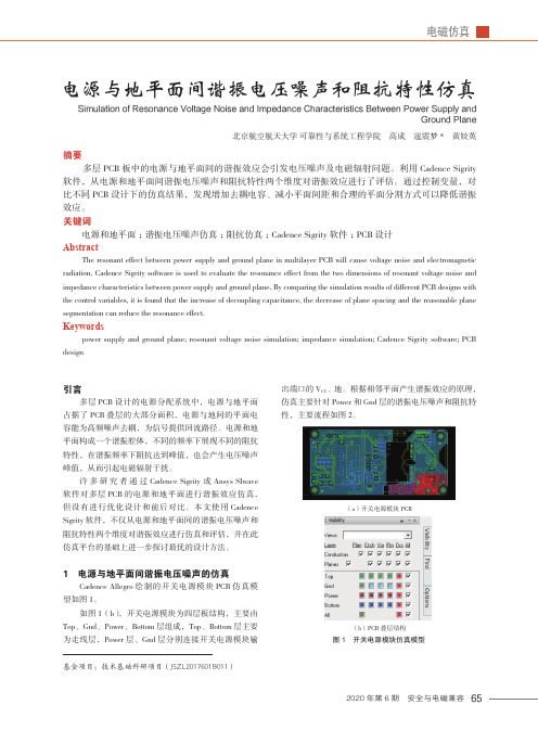
652020年第6期安全与电磁兼容引言多层PCB 设计的电源分配系统中，电源与地平面占据了PCB 叠层的大部分面积，电源与地间的平面电容能为高频噪声去耦，为信号提供回流路径。

电源和地平面构成一个谐振腔体，不同的频率下展现不同的阻抗特性，在谐振频率下阻抗达到峰值，也会产生电压噪声峰值，从而引起电磁辐射干扰。

许多研究者通过Cadence Sigrity 或Ansys SIwave 软件对多层PCB 的电源和地平面进行谐振效应仿真，但没有进行优化设计和前后对比。

本文使用Cadence Sigrity 软件，不仅从电源和地平面间的谐振电压噪声和阻抗特性两个维度对谐振效应进行仿真和评估，并在此仿真平台的基础上进一步探讨最优的设计方法。

1 电源与地平面间谐振电压噪声的仿真Cadence Allegro 绘制的开关电源模块PCB 仿真模型如图1。

如图1（b），开关电源模块为四层板结构，主要由Top、Gnd、Power、Bottom 层组成，Top、Bottom 层主要为走线层，Power 层、Gnd 层分别连接开关电源模块输出端口的V CC 、地。

根据相邻平面产生谐振效应的原理，仿真主要针对Power 和Gnd 层的谐振电压噪声和阻抗特性，主要流程如图2。

摘要多层PCB 板中的电源与地平面间的谐振效应会引发电压噪声及电磁辐射问题。

利用Cadence Sigrity 软件，从电源和地平面间谐振电压噪声和阻抗特性两个维度对谐振效应进行了评估。

通过控制变量，对比不同PCB 设计下的仿真结果，发现增加去耦电容、减小平面间距和合理的平面分割方式可以降低谐振效应。

关键词电源和地平面；谐振电压噪声仿真；阻抗仿真；Cadence Sigrity 软件；PCB 设计AbstractThe resonant effect between power supply and ground plane in multilayer PCB will cause voltage noise and electromagnetic radiation. Cadence Sigrity software is used to evaluate the resonance effect from the two dimensions of resonant voltage noise and impedance characteristics between power supply and ground plane. By comparing the simulation results of different PCB designs with the control variables, it is found that the increase of decoupling capacitance, the decrease of plane spacing and the reasonable plane segmentation can reduce the resonance effect.Keywordspower supply and ground plane; resonant voltage noise simulation; impedance simulation; Cadence Sigrity software; PCB design电源与地平面间谐振电压噪声和阻抗特性仿真Simulation of Resonance Voltage Noise and Impedance Characteristics Between Power Supply andGround Plane北京航空航天大学可靠性与系统工程学院高成寇震梦* 黄姣英（a）开关电源模块PCB（b）PCB 叠层结构图1开关电源模块仿真模型基金项目：技术基础科研项目（JSZL2017601B011）66SAFETY & EMC No.6 2020加载图1的PCB 模型至Cadence Sigrity 模块并检查叠层结构，定义进行仿真的两个平面为Gnd 层和Power 层。

Nonuniform Fast Fourier Transforms Using Min-Max Interpolation

IEEE T-SP, 51(2):560-74, Feb. 2003.
1
Nonuniform Fast Fourier Transforms Using Min-Max Interpolation
Jeffrey A. Fessler∗
4240 EECS, The Unversity of Michigan, Ann Arbor, MI 48109-2122
fessler@ Bradley P. Sutton
BME Department, The University of Michigan
bpsutton@
A BSTRACT The FFT is used widely in signal processing for efﬁcient computation of the Fourier transform (FT) of ﬁnitelength signals over a set of uniformly-spaced frequency locations. However, in many applications, one requires nonuniform sampling in the frequency domain, i.e., a nonuniform FT . Several papers have described fast approximations for the nonuniform FT based on interpolating an oversampled FFT. This paper presents an interpolation method for the nonuniform FT that is optimal in the min-max sense of minimizing the worst-case approximation error over all signals of unit norm. The proposed method easily generalizes to multidimensional signals. Numerical results show that the min-max approach provides substantially lower approximation errors than conventional interpolation methods. The min-max criterion is also useful for optimizing the parameters of interpolation kernels such as the Kaiser-Bessel function. Keywords: Nonuniform FFT, discrete Fourier transform, min-max interpolation, tomography, magnetic resonance imaging, gridding. I. I NTRODUCTION The fast Fourier transform (FFT) is used ubiquitously in signal processing applications where uniformly-spaced samples in the frequency domain are needed. The FFT requires only O(N log N ) operations for an N -point signal, whereas direct evaluation of the discrete Fourier transform requires O(N 2 ) operations. However, a variety of applications require nonuniform sampling in the frequency domain, as has been recognized for at least 30 years [1]. Examples include radar imaging [2–6], computing oriented

切比雪夫多项式公式各项系数

切比雪夫多项式公式各项系数Chebyshev polynomials, named after the Russian mathematician Pafnuty Chebyshev, are a sequence of orthogonal polynomials that are defined over the interval [-1, 1]. These polynomials are widely used in numerical analysis, approximation theory, and other fields due to their excellent approximation properties. The formula for the coefficients of the Chebyshev polynomials involves a recursive relationship that generates the coefficients for each degree of the polynomial.切比雪夫多项式是以俄罗斯数学家帕夫努季·切比雪夫的名字命名的一系列正交多项式，定义在区间[-1, 1]上。

由于其出色的逼近性质，这些多项式在数值分析、逼近理论及其他领域得到广泛应用。

切比雪夫多项式各项系数的公式涉及一个递推关系，通过这个递推关系可以生成每个多项式次数的系数。

Specifically, the coefficients of the Chebyshev polynomial of the first kind, denoted by \(T_n(x)\), are given by the formula:\(T_n(x) = \cos(n \arccos(x))\)when \(n\) is a non-negative integer. This formula expresses the Chebyshev polynomial as a cosine function of a multiple of the arccosine of \(x\). Although this formula is not directly in terms of coefficients, it provides a way to compute the polynomial's values efficiently.具体来说，第一类切比雪夫多项式，记作\(T_n(x)\)，的系数由以下公式给出：\(T_n(x) = \cos(n \arccos(x))\)其中\(n\)是非负整数。

halcon region转正方形

halcon region转正方形In the realm of image processing and analysis, the Halcon library provides a comprehensive set of tools for region manipulation. Among these, the task of converting a region into a square shape often arises, particularly in scenarios where geometric regularization is required. This process, known as region normalization or square conversion, involves altering the shape of the region while preserving its significant features.在图像处理和分析领域，Halcon库提供了一套全面的区域操作工具。

在这些工具中，经常需要将区域转换为正方形形状的任务，特别是在需要几何正则化的场景中。

这个过程被称为区域归一化或正方形转换，它涉及在保留重要特征的同时改变区域的形状。

The key to achieving this transformation lies in understanding the geometric properties of the original region. First, the region's centroid, or center of mass, must be determined. This serves as the pivot point for subsequent operations. Next, the dimensions of the region are analyzed to determine the longest side, which will dictate the size of the resulting square.实现这种转换的关键在于理解原始区域的几何属性。

八十词关于电脑是一项意外发明的英语作文

八十词关于电脑是一项意外发明的英语作文全文共3篇示例，供读者参考篇1Computer is an accidental invention, which has greatly changed our lives in the past few decades. It was not designed specifically as a machine for personal or professional use, but rather as a military tool during World War II. In 1941, the Atanasoff-Berry Computer, the first electronic computer, was developed by John Vincent Atanasoff and Clifford Berry at Iowa State College. This invention laid the foundation for the development of modern computers.In the following years, many developments and advancements were made in the field of computer technology. The invention of the transistor, integrated circuit, and microprocessor revolutionized the computer industry. These advancements made computers smaller, faster, and more powerful, leading to the proliferation of personal computers in homes and workplaces.The introduction of the internet in the 1990s further revolutionized the way we use computers. It connected peopleall over the world and made information more accessible than ever before. Today, computers are an integral part of our daily lives, from communicating with others and accessing information to entertainment and work.In conclusion, the accidental invention of the computer has had a profound impact on society and has changed the way we live, work, and communicate. It is hard to imagine a world without computers and the technology that has evolved from this accidental invention.篇2Computers are now an essential part of our daily lives, but it may surprise you to learn that they were actually an accidental invention. In the 19th century, mathematician and inventor Charles Babbage came up with the concept of a mechanical computer, which he called the Analytical Engine. However, due to limitations in technology at the time, he was never able to build a working model.It wasn't until the mid-20th century that the modern computer as we know it was born. During World War II, the need for fast and efficient computation led to the development of the first electronic computers. These early computers were massive,slow, and often unreliable, but they laid the foundation for the technology that would eventually revolutionize the world.In 1947, the first truly modern computer was developed. The Electronic Numerical Integrator and Computer (ENIAC) was a massive machine that could perform complex calculations at incredible speed. It was a breakthrough in computing technology, and it paved the way for the development of smaller, faster, and more powerful computers.Since then, computers have evolved at a rapid pace. From the desktop computers of the 1980s to the laptops, tablets, and smartphones of today, computing technology has become an integral part of modern society. We use computers for work, communication, entertainment, and so much more.It's amazing to think that this incredible technology was born out of a series of accidents and innovations. Without the curiosity and ingenuity of inventors like Charles Babbage and the need for fast computation during World War II, we might never have had the computers that are now so essential to our daily lives.In conclusion, the computer is truly an accidental invention that has changed the world in ways that no one could have predicted. Its evolution from a concept in the 19th century to theubiquitous technology of today is a testament to human ingenuity and the power of innovation. Without computers, the modern world would be a very different place, and it's exciting to think about what new developments in computing technology lie ahead.篇3Computer is an accidental invention that has transformed the way we live and work. The first programmable computer, the Colossus, was created during World War II for code-breaking purposes. Since then, computers have evolved significantly, becoming smaller, faster, and more powerful.The invention of the personal computer in the 1970s marked a major milestone in the history of technology. With the introduction of user-friendly interfaces and software, computers became more accessible to the general public. This led to the rise of the digital age and the internet, changing the way we communicate, shop, and gather information.Today, computers are an essential part of our daily lives, used in everything from education and healthcare to banking and entertainment. They have revolutionized industries and created new opportunities for innovation and growth. Despitebeing an accidental invention, the computer has had a profound impact on society and will continue to shape our future.。

算盘老物件作文

The Abacus: A Timeless ArtifactThe abacus, a time-honored tool of ancient Chinese mathematics, remains a fascinating relic of the past. This wooden calculator, with its intricate sliding beads and wires, is a testament to the ingenious minds of the ancient Chinese, who devised a means of computation that was both efficient and accurate.The abacus dates back to the Zhou dynasty, over 3,000 years ago, and has since been used by generations of Chinese scholars and merchants. Its design, simple yet elegant, allowed for complex calculations to be performed quickly, making it an invaluable tool in business transactions and academic pursuits.What sets the abacus apart from other calculators is its unique method of computation. The beads, which slide up and down on wires, represent numbers in a binary system, with the upper beads representing 5 and the lower beads representing 1. This system allows for quick and efficient addition, subtraction, multiplication, and even division.The abacus's enduring popularity can be attributed to its portability and durability. Made from hardwood, it was designed to withstand the rigors of daily use, making it a practical tool for merchants on the go. Its small size also meant that it could easily be tucked away into a bag or pouch, allowing users to carry it wherever they needed to perform calculations.Today, while the abacus has been superseded by more modern and sophisticated calculators and computers, it remains a cherished artifact of Chinese culture. Its presence in museums and private collections serves as a reminder of the remarkable achievements of ancient Chinese mathematicians and engineers.算盘：跨越时空的老物件算盘，这一古代中国数学的标志性工具，至今仍是令人着迷的历史遗物。

anf 文法

ANF (Acyclic Normal Form) is a data format used in computer systems to represent complex data structures as a directed acyclic graph (DAG) or a tree. It is primarily utilized in the context of compilers, programming languages, and variousoptimization techniques.In ANF, the graph is designed to be acyclic, which means it does not contain any cycles or loops. This design choice simplifies the analysis and manipulation of the data structure, making it easier to reason about and optimize.The ANF format provides several benefits compared to other representations, such as:1.Simplified structure: ANF eliminates the need for explicit loops orrecursion, resulting in a simpler and more straightforward data structure. This simplification aids in the analysis and transformation of the data, improvingcompiler optimizations and static analysis techniques.2.Sharing of common subexpressions: ANF facilitates the identificationand sharing of common subexpressions within the data structure. This sharing reduces redundancy and improves memory efficiency. By representingcommon subexpressions as shared nodes in the graph, ANF optimizes thestorage and computation required to represent complex expressions.3.Efficient evaluation: ANF provides an efficient evaluation strategy byordering the computation of expressions within the graph. The order ofevaluation is determined by the dependencies among the nodes in the graph.This strategy ensures that each expression is computed only once and thatdependencies are satisfied before their use. Consequently, ANF enables efficient and optimized evaluation of complex expressions.nguage independence: ANF is independent of any specificprogramming language or compiler. It is a general-purpose data format thatcan be used to represent various kinds of data structures and expressions. This language independence makes ANF widely applicable and adaptable todifferent programming paradigms and optimization techniques.5.Versatility: ANF can represent a wide range of data structures andexpressions, including arithmetic expressions, control flow structures,functional abstractions, and more. It is a flexible and adaptable format that can capture complex program structures in a concise and efficient manner.6.Debugging and analysis: By representing complex data structures as adirected acyclic graph, ANF enables easier debugging and analysis of programs.The acyclic nature of the graph simplifies the identification of problematicareas and aids in the understanding of program behavior.In conclusion, ANF is a data format that represents complex data structures as a directed acyclic graph (DAG) or a tree. It provides benefits such as simplifiedstructure, sharing of common subexpressions, efficient evaluation, language independence, versatility, and improved debugging and analysis capabilities. Utilizing ANF can enhance the performance, efficiency, and understandability of programs, making it an essential tool in compilers, programming languages, and optimization techniques.。

1、下载文档前请自行甄别文档内容的完整性，平台不提供额外的编辑、内容补充、找答案等附加服务。
2、"仅部分预览"的文档,不可在线预览部分如存在完整性等问题,可反馈申请退款(可完整预览的文档不适用该条件!)。
3、如文档侵犯您的权益，请联系客服反馈,我们会尽快为您处理(人工客服工作时间：9:00-18:30)。

uses completely disconnected subgraphs as the dividing boundary for forming subgraphs.
3: The Johnson Representation Polynomial
Johnson [3] deﬁned the representation polynomial as: n i P ( X, z ) = a ( X, i ) z (2) i=1 where n is the order of X and a(X,i) is the number of ivalued representations of X. That is, a(X,i) is the number of linear extensions of length i of X. Thus, the representation polynomial of a chain graph Cn (height n-1) is given by: ( z ) = z (1 + z)n-1. C n For an arbitrary directed acyclic graph, representation polynomial may be determined decomposing the graph into a series of chain graphs combining the polynomial of all the chain graphs as: P (3) the by and
∑
do check current graph for antichain if (antichain = not found) check for chain if (chain and antichain = not found) numfree = number of free vertices if (numfree = 2) free1 = ﬁrst free vertex free2 = second free vertex create new subgraphs current graph = last new graph if (numfree = 1) remove free vertex and edges else if (chain = found) add chain polynomial to total polynomial else determine antichain polynomial add antichain polynomial to total polynomial if (ﬁnished) continue = FALSE else free unneeded memory current graph = current graph - 1 continue = TRUE while continue = TRUE

1: Introduction
Much research has been done in the analysis of graphs as they apply to mapping application algorithms to parallel architectures. Many allocation heuristics rely on information obtained from analyzing task graph characteristics. It is hypothesized that information useful in predicting the behavior of task graph mappings is contained in the representation polynomial of a task graph. As stated, the representation polynomial, developed by K. Johnson [3], is a mathematical equation corresponding to a directed acyclic graph. Some properties of the representation polynomial are well established including: a representation of the graph order via the degree of the polynomial, graph height determination via multiplicity of polynomial roots, and information derived from coefﬁcients of the terms of the polynomial. Additional characteristics and proofs regarding the polynomial are given by Johnson and Neggers. It is suspected that information valuable in directing heuristic allocation
algorithms can be obtained by studying the representation polynomials of many classes of graphs. This paper describes brieﬂy graph theory terminology used, the representation polynomial, Johnson’s algorithm for polynomial computation, and enhancements to the algorithm. The algorithm enhancements include cardinal and ordinal graph simpliﬁcation, techniques for chain and antichain graph detection, and efﬁcient memory allocation and deallocation schemes for decomposed graphs. All enhancements are utilized for improved computational efﬁciency resulting a more robust algorithm capable of operating on large, complex graphs.
Abstract
The representation polynomial, developed by K. Johnson, is a mathematical equation corresponding to a directed acyclic graph. Johnson’s algorithm is based on decomposing the graph into a set of chain graphs which have a known equation for the representation polynomial. However, the analysis time and computer memory requirements for calculating the representation polynomial for an arbitrary graph of more than ten vertices, from previous implementations [6] of Johnson’s algorithm, is beyond reasonable bounds. Consequently, modiﬁcations are made to the implementation of Johnson’s algorithm to decrease the required computation time as well as optimize the allocation of available computer memory. The approach and related results described include antichain graph detection, enhanced chain graph detection, dynamic memory allocation, and graph simpliﬁcation.
Computing the Representation Polynomial for Directed Acyclic Graphs Using Subgraph Detection and Simpliﬁcation
David Jeff Jackson and Chris Humphres Department of Electrical Engineering The University of Alabama, Tuscaloosa, AL 35487
2: Graph Theory Terminology
A description of graph theory terminology utilized in this paper follows. A graph is deﬁned to be a pair (X, U), where X is a set {x1, x2,..., xn} of elements referred to as vertices, and U is a family (u1, u2,..., um) of elements of the Cartesian product X*X, referred to as arcs [1-2]. The degree of a vertex, dG(x), is the number of arcs incident to x [5]. The number of arcs incident out of a vertex, the outer demi-degree, is denoted as dG+(x). The number of arcs incident into a vertex, the inner demi-degree, is denoted as dG-(x). The degree of a vertex x is thus given as: + d ( x) = d ( x) + d ( x) . (1) G G G A vertex is isolated, i.e. a singleton, if dG(x) = 0. The number of vertices in a graph is the order of the graph. A vertex such that dG-(x) = 0 is referred to as a no-entry or a free vertex. Two free vertices in a graph constitute a free pair and the rank r(x) of a graph X is the number of pairs (A, B) of free vertices in X [3]. Finally, a subgraph of a graph G is a graph H such that every vertex of H is a vertex of G, and every arc of H is an arc of G [6]. Two methods of dividing graphs into subgraphs described are cardinal and ordinal reduction. Ordinal reduction uses completely connected bipartite graphs as the dividing boundary and cardinal reduction