1 Signal and System
信号与系统基本概念
1
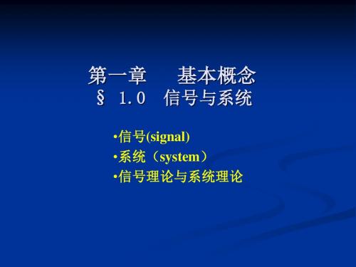
p( t )
2
O
2
t
面积1; 脉宽↓; 脉冲高度↑; 则窄脉冲集中于 t=0 处。 ★面积为1 三个特点: ★宽度为0
无穷 ★ 幅度 0
t0 t0
1 ( t ) lim p( t ) lim u t u t 0 0 2 2
系统
输出信号 响应
通信系统:为传送消息而装设的全套技术设备 (包括传输信道)。
信息 源 发送 设备 信道 接收 设备 受信 者
发送端 消息 信号
噪声 源 信号
接收端 消息
§1.1 信号的描述和分类
•信号的描述
•信号的分类
一、信号的描述
描述方法:(1)数学表达式 (2)波形图 (3)频谱图 (4)测量与统计数据
冲激函数的性质
t 函数,它属于广 为了信号分析的需要,人们构造了 t 而言, t 可以当作时域连续信号处 义函数。就时间
理,因为它符合时域连续信号运算的某些规则。但由于 t 是一个广义函数,它有一些特殊的性质。
1.抽样性 2.奇偶性
抽样性(筛选性)
如果f(t)在t = 0处连续,且处处有界,则有
(t )具有筛选f (t )在t 0处函数值的性质 (t t0 )具有筛选f (t )在t t0处函数值的性质
(t ) ( t )
奇偶性
•由定义2,矩形脉冲本身是偶函数,故极限 也是偶函数。
•由抽样性证明奇偶性。
(t ) f (t ) d t f (0)
( t ) f ( t ) f (0) ( t )
Chapter1 Signals and Systems
Example Fig 3
1.2 Transformations of The independent Variable
1.2.3 Even and Odd Signals
1.2 Transformations of The indepenຫໍສະໝຸດ ent Variable2
The total energy over an infinite time interval in discrete-time is defined as:
E lim
N n N
| x[n] |
2
N
n
| x[n] |2
1.1 Continuous-time and Discretetime Signals
Preface
◆Chapter1
Signals and Systems
◆ Chapter2
◆ Chapter3
Linear Time-invariant Systems
Fourier Series representation of periodic
signals
◆ Chapter4 ◆ Chapter5
Sinusoidal Signals(正弦信号):
1.3 Exponential And Sinusoidal Signals
1.3.1 Continuous-time Complex Exponential and Sinusoidal Signals
Sinusoidal Signals(正弦信号):
1 [ n] 0 n0 n0
1
[n]
2
signal and system 英文原版书

signal and system 英文原版书Title: An Overview of the Book "Signal and System"Introduction:The book "Signal and System" is an essential resource for anyone interested in understanding the fundamentals of signal processing and system analysis. It provides a comprehensive and in-depth exploration of the concepts, theories, and applications related to signals and systems. This article aims to provide a detailed overview of the book, highlighting its key points and relevance.I. Fundamental Concepts of Signals and Systems:1.1 Definition and Properties of Signals:- Explanation of signals as time-varying or spatially varying quantities.- Discussion on continuous-time and discrete-time signals.- Description of signal properties such as amplitude, frequency, and phase.1.2 Classification of Signals:- Overview of different types of signals including periodic, aperiodic, deterministic, and random signals.- Explanation of energy and power signals.- Introduction to common signal operations such as time shifting, scaling, and time reversal.1.3 System Classification and Properties:- Definition and classification of systems as linear or nonlinear, time-invariant or time-varying.- Explanation of system properties like causality, stability, and linearity.- Introduction to system representations such as differential equations, transfer functions, and state-space models.II. Time-Domain Analysis of Signals and Systems:2.1 Convolution and Correlation:- Detailed explanation of convolution and its significance in system analysis.- Discussion on correlation as a measure of similarity between signals.- Application of convolution and correlation in practical scenarios.2.2 Fourier Series and Transform:- Introduction to Fourier series and its representation of periodic signals.- Explanation of Fourier transform and its application in analyzing non-periodic signals.- Discussion on the properties of Fourier series and transform.2.3 Laplace Transform:- Overview of Laplace transform and its use in solving differential equations.- Explanation of the relationship between Laplace transform and frequency response of systems.- Application of Laplace transform in system analysis and design.III. Frequency-Domain Analysis of Signals and Systems:3.1 Frequency Response:- Definition and interpretation of frequency response.- Explanation of magnitude and phase response.- Analysis of frequency response using Bode plots.3.2 Filtering and Filtering Techniques:- Introduction to digital and analog filters.- Discussion on different filter types such as low-pass, high-pass, band-pass, and band-stop filters.- Explanation of filter design techniques including Butterworth, Chebyshev, and Elliptic filters.3.3 Sampling and Reconstruction:- Explanation of sampling theorem and its importance in signal processing.- Overview of sampling techniques and their impact on signal reconstruction.- Discussion on anti-aliasing filters and reconstruction methods.IV. System Analysis and Stability:4.1 System Response and Impulse Response:- Explanation of system response to different input signals.- Introduction to impulse response and its relationship with system behavior.- Analysis of system stability based on impulse response.4.2 Transfer Function and Frequency Domain Analysis:- Definition and interpretation of transfer function.- Explanation of frequency domain analysis using transfer function.- Application of transfer function in system design and analysis.4.3 Feedback Systems and Control:- Overview of feedback systems and their role in control theory.- Explanation of stability analysis and design using control theory.- Discussion on PID controllers and their applications.V. Applications of Signal and System Theory:5.1 Communication Systems:- Explanation of modulation techniques and their role in communication systems.- Overview of demodulation techniques and their significance.- Discussion on error control coding and channel equalization.5.2 Digital Signal Processing:- Introduction to digital signal processing and its applications.- Explanation of digital filters and their role in signal processing.- Overview of image and speech processing techniques.5.3 Signal Processing in Biomedical Engineering:- Application of signal processing in biomedical signal analysis.- Discussion on medical imaging techniques such as MRI and CT scans.- Explanation of signal processing methods used in ECG and EEG analysis.Conclusion:The book "Signal and System" provides a comprehensive and detailed exploration of the fundamental concepts, theories, and applications related to signals and systems. It covers a wide range of topics including signal classification, system analysis, frequency-domain analysis, stability, and various applications. By studying this book, readers can gain a solid understanding of signal and system theory, which is essential in various fields such as communication, digital signal processing, and biomedical engineering.。
Signals and Systems - Shandong University
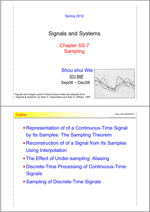
Spring 2012Signals and SystemsChapter SS-7 SamplingShou shui Wei SDU-BMESep08 – Dec08Figures and images used in these lecture notes are adopted from “Signals & Systems” by Alan V. Oppenheim and Alan S. Willsky, 1997OutlineShou shui Wei©2012 Representation of of a Continuous-Time Signal by Its Samples: The Sampling Theorem Reconstruction of of a Signal from Its Samples Using Interpolation The Effect of Under-sampling: Aliasing Discrete-Time Processing of Continuous-TimeSignals Sampling of Discrete-Time SignalsThe Sampling TheoremShou shui Wei©2012 Representation of CT Signals by its SamplesThe Sampling TheoremShou shui Wei©2012 Representation of CT Signals by its SamplesThe Sampling TheoremShou shui Wei©2012 Representation of CT Signals by its SamplesThe Sampling Theorem Impulse-Train Sampling:Shou shui Wei©2012The Sampling Theorem Impulse-Train Sampling:Eq 4.70, p. 322Shou shui Wei©2012Ex 4.21, p. 323Ex 4.8, pp. 299-300The Sampling Theorem Impulse-Train Sampling:Shou shui Wei©2012Ex 4.21, 4.22, pp. 323-4The Sampling Theorem The Sampling Theorem:Shou shui Wei©2012The Sampling TheoremShou shui Wei©2012 Exact Recovery by an Ideal Lowpass Filter:The Sampling Theorem Sampling with Zero-Order Hold:Shou shui Wei©2012The Sampling TheoremShou shui Wei©2012 Sampling with Zero-Order Hold: Ex 4.4, p. 293Eq 4.27, p. 301OutlineShou shui Wei©2012 Representation of of a Continuous-Time Signal by Its Samples: The Sampling Theorem Reconstruction of of a Signal from Its Samples Using Interpolation The Effect of Under-sampling: Aliasing Discrete-Time Processing of Continuous-TimeSignals Sampling of Discrete-Time SignalsReconstruction of a Signal from its Samples Using Interpolation Shou shui Wei©2012 Exact Interpolation:Ex 2.11, p. 110Reconstruction of a Signal from its Samples Using Interpolation Shou shui Wei©2012 Exact Interpolation:Reconstruction of a Signal from its Samples Using Interpolation Shou shui Wei©2012 Ideal Interpolating Filter & The Zero-Order Hold:Reconstruction of a Signal from its Samples Using Interpolation Shou shui Wei©2012 Sampling & Interpolation of Images:Reconstruction of a Signal from its Samples Using Interpolation Shou shui Wei©2012 Higher-Order Holds:Reconstruction of a Signal from its Samples Using Interpolation Shou shui Wei©2012 Higher-Order Holds:Ex 4.4, p. 293=*=XReconstruction of a Signal from its Samples Using Interpolation Shou shui Wei©2012 First-Order Hold on Image Processing:OutlineOverlapping in Frequency-Domain: AliasingOverlapping in Frequency-Domain: AliasingEffect of Under-sampling: AliasingOverlapping in Frequency-Domain: AliasingStrobe Effect: OutlineShou shui Wei©2012 Discrete-Time Processing of Continuous-Time SignalsEq7.3, 7.6, p. 517Shou shui Wei©2012 Discrete-Time Processing of Continuous-Time SignalsFrequency-Domain Illustration:1Frequency-Domain Illustration:Shou shui Wei©2012 Discrete-Time Processing of Continuous-Time SignalsCT & DT Frequency Responses:OutlineImpulse-Train Sampling:Exact Recovery Using Ideal Lowpass Filter:Higher Equivalent Sampling Rate: Up-sampling。
信号与系统目录(Signal and system directory)
信号与系统目录(Signal and system directory)Chapter 1 signals and systems1.1 INTRODUCTION1.2 signalContinuous signals and discrete signalsTwo. Periodic signals and aperiodic signalsThree, real signal and complex signalFour. Energy signal and power signalThe basic operation of 1.3 signalAddition and multiplicationTwo, inversion and TranslationThree, scale transformation (abscissa expansion)1.4 step function and impulse functionFirst, step function and impulse functionTwo. Definition of generalized function of impulse functionThree. The derivative and integral of the impulse functionFour. Properties of the impulse functionDescription of 1.5 systemFirst, the mathematical model of the systemTwo. The block diagram of the systemCharacteristics and analysis methods of 1.6 systemLinearTwo, time invarianceThree, causalityFour, stabilityOverview of five and LTI system analysis methodsExercise 1.32The second chapter is the time domain analysis of continuous systemsThe response of 2.1LTI continuous systemFirst, the classical solution of differential equationTwo, about 0- and 0+ valuesThree, zero input responseFour, zero state responseFive, full response2.2 impulse response and step responseImpulse responseTwo, step response2.3 convolution integralConvolution integralTwo. The convolution diagramThe properties of 2.4 convolution integralAlgebraic operations of convolutionTwo. Convolution of function and impulse function Three. Differential and integral of convolutionFour. Correlation functionExercise 2.34The third chapter is the time domain analysis of discretesystemsThe response of 3.1LTI discrete systemsDifference and difference equationsTwo. Classical solutions of difference equationsThree, zero input responseFour, zero state response3.2 unit sequence and unit sequence responseUnit sequence and unit step sequenceTwo, unit sequence response and step response3.3 convolution sumConvolution sumTwo. The diagram of convolution sumThree. The nature of convolution sum3.4 deconvolutionExercise 3.27The fourth chapter is Fourier transform and frequency domainanalysis of the systemThe 4.1 signal is decomposed into orthogonal functions Orthogonal function setTwo. The signal is decomposed into orthogonal functions 4.2 Fourier seriesDecomposition of periodic signalsTwo, Fourier series of odd even functionThree. Exponential form of Fu Liye seriesThe spectrum of 4.3 period signalFrequency spectrum of periodic signalTwo, the spectrum of periodic matrix pulseThree. The power of periodic signal4.4 the spectrum of aperiodic signalsFirst, Fu Liye transformTwo. Fourier transform of singular functionsProperties of 4.5 Fourier transformLinearTwo, parityThree, symmetryFour, scale transformationFive, time shift characteristicsSix, frequency shift characteristicsSeven. Convolution theoremEight, time domain differential and integral Nine, frequency domain differential and integral Ten. Correlation theorem4.6 energy spectrum and power spectrumEnergy spectrumTwo. Power spectrumFourier transform of 4.7 periodic signals Fourier transform of sine and cosine functionsTwo. Fourier transform of general periodic functionsThree 、 Fu Liye coefficient and Fu Liye transformFrequency domain analysis of 4.8 LTI systemFrequency responseTwo. Distortionless transmissionThree. The response of ideal low-pass filter4.9 sampling theoremSampling of signalsTwo. Time domain sampling theoremThree. Sampling theorem in frequency domainFourier analysis of 4.10 sequencesDiscrete Fourier series DFS of periodic sequencesTwo. Discrete time Fourier transform of non periodic sequences DTFT4.11 discrete Fu Liye and its propertiesDiscrete Fourier transform (DFT)Two. The properties of discrete Fourier transformExercise 4.60The fifth chapter is the S domain analysis of continuous systems 5.1 Laplasse transformFirst, from Fu Liye transform to Laplasse transformTwo. Convergence domainThree, (Dan Bian) Laplasse transformThe properties of 5.2 Laplasse transformLinearTwo, scale transformationThree, time shift characteristicsFour, complex translation characteristicsFive, time domain differential characteristicsSix, time domain integral characteristicsSeven. Convolution theoremEight, s domain differential and integralNine, initial value theorem and terminal value theorem5.3 Laplasse inverse transformationFirst, look-up table methodTwo, partial fraction expansion method5.4 complex frequency domain analysisFirst, the transformation solution of differential equation Two. System functionThree. The s block diagram of the systemFour 、 s domain model of circuitFive, Laplasse transform and Fu Liye transform5.5 bilateral Laplasse transformExercise 5.50The sixth chapter is the Z domain analysis of discrete systems 6.1 Z transformFirst, transform from Laplasse transform to Z transformTwo, z transformThree. Convergence domainProperties of 6.2 Z transformLinearTwo. Displacement characteristicsThree, Z domain scale transformFour. Convolution theoremFive, Z domain differentiationSix, Z domain integralSeven, K domain inversionEight, part sumNine, initial value theorem and terminal value theorem 6.3 inverse Z transformFirst, power series expansion methodTwo, partial fraction expansion method6.4 Z domain analysisThe Z domain solution of difference equationTwo. System functionThree. The Z block diagram of the systemFour 、 the relation between s domain and Z domainFive. Seeking the frequency response of discrete system by means of DTFTExercise 6.50The seventh chapter system function7.1 system functions and system characteristicsFirst, zeros and poles of the system functionTwo. System function and time domain responseThree. System function and frequency domain responseCausality and stability of 7.2 systemsFirst, the causality of the systemTwo, the stability of the system7.3 information flow graphSignal flow graphTwo, Mason formulaStructure of 7.4 systemFirst, direct implementationTwo. Implementation of cascade and parallel connectionExercise 7.39The eighth chapter is the analysis of the state variables of the system8.1 state variables and state equationsConcepts of state and state variablesTwo. State equation and output equationEstablishment of state equation for 8.2 continuous systemFirst, the equation is directly established by the circuit diagramTwo. The equation of state is established by the input-output equationEstablishment and Simulation of state equations for 8.3discrete systemsFirst, the equation of state is established by the input-output equationTwo. The system simulation is made by the state equationSolution of state equation of 8.4 continuous systemFirst, the Laplasse transform method is used to solve the equation of stateTwo, the system function matrix H (z) and the stability of the systemThree. Solving state equation by time domain methodSolution of state equation for 8.5 discrete systemsFirst, the time domain method is used to solve the state equations of discrete systemsTwo. Solving the state equation of discrete system by Z transformThree, the system function matrix H (z) and the stability of the systemControllability and observability of 8.6 systemsFirst, the linear transformation of state vectorTwo, the controllability and observability of the systemExercise 8.32Appendix a convolution integral tableAppendix two convolution and tableAppendix three Fourier coefficients table of commonly used periodic signalsAppendix four Fourier transform tables of commonly used signalsAppendix five Laplasse inverse exchange tableAppendix six sequence of the Z transform table。
信号与系统SignalsandSystemsppt课件
0.5
0.4
0.3
0.2
0.1
0
0
1
2
3
4
5
6
7
8
9
10
1
0.9
0.8
0.7
0.6
0.5
0.4
0.3
0.2
0.1
0
0
1
2
3
4
5
6
7
8
9
10
一、基本信号的MATLAB表示
% rectpuls
t=0:0.001:4; T=1; ft=rectpuls(t-2*T,T); plot(t,ft) axis([0,4,-0.5,1.5])
rand
产生(0,1)均匀分布随机数矩阵
randn 产生正态分布随机数矩阵
四、数组
2. 数组的运算
数组和一个标量相加或相乘 例 y=x-1 z=3*x
2个数组的对应元素相乘除 .* ./ 例 z=x.*y
确定数组大小的函数 size(A) 返回值数组A的行数和列数(二维) length(B) 确定数组B的元素个数(一维)
0.3
0.2
0.1
function [f,k]=impseq(k0,k1,k2) 0
-50 -40 -30 -20 -10
0
10 20 30 40 50
%产生 f[k]=delta(k-k0);k1<=k<=k2
k=[k1:k2];f=[(k-k0)==0];
k0=0;k1=-50;k2=50;
[f,k]=impseq(k0,k1,k2);
已知三角波f(t),用MATLAB画出的f(2t)和f(2-2t) 波形
Signals1

23
1 Signal and System
1.3 Exponential and Sinusoidal Signals 1.3.1 Continuous-Time Complex x( t ) Ce at Exponential and Sinusoidal Signals
8
1 Signal and System
Types of Signals Continuous-time Signal
9
1 Signal and System
Discrete-time Signal
10
1 Signal and System
Representation Function Representation Example: x(t) = cos0t
x[n] cos 0n
Graphical Representation
(2) Graphical Representation
11
1 Signal and System
1.1.2 Signal Energy and Power Instantaneous power: 1 2 p(t ) v(t ) i (t ) v (t ) R i 2 (t ) R Energy over t t t : 1 2
Real Exponential Signals C and a are real.
a0
a0
24
1 Signal and System
Periodic Complex Exponential and Sinusoidal Signals a is purely imaginary.
signals and systems_introduction

I(x,y)
What is a Signal (信号)?
Definitions A Signal is formally defined as a function of one or more variables that conveys information on the nature of a physical phenomenon. 信号是一个或多个变量的函数,携带着某个物 理现象的信息。
3. Four different forms of Fourier Transform:
Continuous and Periodic Discrete and Periodic Continuous and Aperiodic Discrete and Aperiodic
4. Use the right one !!!
第三章 信号与线性非时变系统的傅里叶分析 (Fourier Representations for signals and Linear TimeInvariant Systems ) 离散时间周期与非周期信号、连续时间周期与非周期信号的傅里叶分析; 傅里叶分析的性质;LTI系统的频域分析。
Contents
Signals and Systems
--- One of the most important courses for us!
陈布雨 技术中心B区217室 图书馆720
Contents
第一章 信号与系统简介 (Introduction) 介绍信号与系统的基本概念; 信号分类及基本信号;系统分类和特性。 第二章 线性非时变系统的时域分析 (Time-Domain Representations for Linear TimeInvariant Systems) 单位冲激响应和单位脉冲响应,卷积积分和卷积和;系统的互联;系统 的响应求解;系统的方框图表示, 系统的状态空间分析。
1信号与系统英语课件

| 信
号 与
系
统
电 子
与
信
息
罗
学
劲
院
洪 薛 洋
What is a System
| 信
A System is formally defined as an entity that manipulates 号 one or more signals to accomplish a function, thereby 与 yielding new signals.
号
1 xo (t ) [ x(t ) x(t )] 2
与
系
统
电 子
与
信
息
罗
学
劲
院
洪 薛 洋
EX3:
x(t )
2 1 -2 -1 0 1 2
| 信
t
-2
xe (t )
1 0 2
xo (t )
1 -1
-1 1
号
t
t与
系
统
电 子
与
信
息
罗
学
劲
院
洪 薛 洋
| 信 1.continuous-time complex exponential and sinusoidal signals
t2
| 信
号 与
t1
| x(t ) |2 dt
n2
Over the time interval [n1,n2], the total energy of x[n] is:
E=
n n1 2 | x [ n ] |
系
2
Definitions 能量信号
E lim x(t ) dt E lim n
电子科大信号系统英文课件Chapter1 SignalandSystem-B
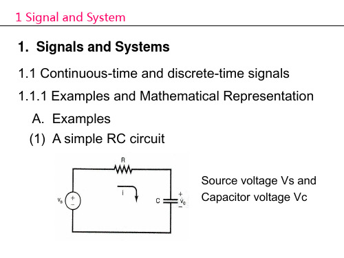
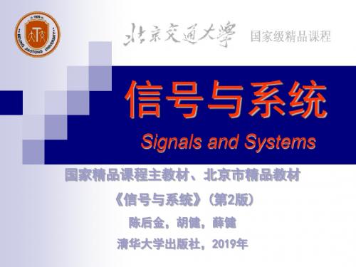
1. Signals and Systems 1.1 Continuous-time and discrete-time signals 1.1.1 Examples and Mathematical Representation
A. Examples (1) A simple RC circuit
(3) A Speech Signal
1 Signal and System
(4) A Picture
1 Signal and System
(5) Vertical Wind Profile
1 Signal and System
B. Types of Signals (1) Continuous-time Signal
1 Signal and System
Energy over t1 t t2:
t2p(t)dt t2v2 (t)dt t2x2 (t)dt
t1
t1
t1
Total Energy:
lim E T
t2x2 (t)dt
t1
lim Average Power:
P
T
1 2T
T x2 (t)dt
Right shift : x(t-t0) x[n-n0]
Left shift : x(t+t0) x[n+n0]
(Delay) (Advance)
1 Signal and System Examples
1 Signal and System
B. Time Reversal x(-t) or x[-n] : Reflection of x(t) or x[n]
(完整版)奥本海姆信号与系统第二版英文课件第一章
1 Signal and System Examples of periodic signal
1 Signal and System
1.2.3 Even and Odd Signals
1.2.1 Examples of Transformations A. Time Shift
Right shift : x(t-t0) x[n-n0]
Left shift : x(t+t0) x[n+n0]
(Delay) (Advance)
1 Signal and System Examples
Even signal: x(-t) = x(t) or x[-n]= x[n] Odd signal : x(-t)= -x(t) or x[-n]= -x[n]
Even-Odd Decomposition:
Ev{x(t )}
xe (t)
1 [x(t) 2
x(t )]
Od {x(t )}
xo (t)
1 Signal and System
B. Time Reversal x(-t) or x[-n] : Reflection of x(t) or x[n]
1 Signal and System
C. Time Scaling
x(at) ( a>0 )
Stretch
if a<0
Compressed if a>0
T x2 (t)dt
T
1 Signal and System
signals and systems
S T R U C T U R E A N DI N T E R P R E T A T I O N O FSignals andSystemsEdward A.LeePravin VaraiyaUNIVERSITY OF CALIFORNIA AT BERKELEYPrefaceT his textbook is about signals and systems,a discipline rooted in the in-tellectual tradition of electrical engineering(EE).This tradition,however,hasevolved in unexpected ways.EE has lost its tight coupling with the“electrical.”Electricity provides the impetus,the potential,but not the body of the subject.How else could microelectromechanical systems(MEMS)become so importantin EE?Is this not mechanical engineering?Or signal processing?Is this not mathe-matics?Or digital networking?Is this not computer science?How is it that controlsystem techniques are profitably applied to aeronautical systems,structural me-chanics,electrical systems,and options pricing?This book approaches signals and systems from a computational point ofview.It is intended for students interested in the modern,highly digital problemsof electrical engineering,computer science,and computer engineering.In par-ticular,the approach is applicable to problems in computer networking,wirelesscommunication systems,embedded control,audio and video signal processing,and,of course,circuits.A more traditional introduction to signals and systems would be biasedtoward the latter application,circuits.It would focus almost exclusively on lineartime-invariant systems,and would develop continuous-time modelsfirst,withdiscrete-time models then treated as an advanced topic.The discipline,after all,grew out of the context of circuit analysis.But it has changed.Even pure EExiiixiv Prefacegraduates are more likely to write software than to push electrons,and yet westill recognize them as electrical engineers.The approach in this book benefits students by showing from the start that the methods of signals and systems are applicable to software systems,andmost interestingly,to systems that mix computers with physical devices such ascircuits,mechanical control systems,and physical media.Such systems havebecome pervasive,and profoundly affect our daily lives.The shift away from circuits implies some changes in the way the method-ology of signals and systems is presented.While it is still true that a voltage thatvaries over time is a signal,so is a packet sequence on a network.This text de-fines signals to cover both.While it is still true that an RLC circuit is a system,so is a computer program for decoding Internet audio.This text defines systemsto cover both.While for some systems the state is still captured adequately byvariables in a differential equation,for many it is now the values in registers andmemory of a computer.This text defines state to cover both.The fundamental limits also change.Although we still face thermal noise and the speed of light,we are likely to encounter other limits—such as complexity,computability,chaos,and,most commonly,limits imposed by other humanconstructions—before we get to these.A voiceband data modem,for example,uses the telephone network,which was designed to carry voice,and offers asimmutable limits such nonphysical constraints as its3kHz bandwidth.This hasno intrinsic origin in the physics of the network;it is put there by engineers.Similarly,computer-based audio systems face latency and jitter imposed by theoperating system.This text focuses on composition of systems so that the limitsimposed by one system on another can be understood.The mathematical basis for the discipline also changes.Although we still use calculus and differential equations,we frequently need discrete math,set theory,and mathematical logic.Whereas the mathematics of calculus and differentialequations evolved to describe the physical world,the world we face as systemdesigners often has nonphysical properties that are not such a good match forthis mathematics.This text bases the entire study on a highly adaptable formalismrooted in elementary set theory.Despite these fundamental changes in the medium with which we operate, the methodology of signals and systems remains robust and powerful.It is themethodology,not the medium,that defines thefield.The book is based on a course at Berkeley taught over the past four years to more than2,000students in electrical engineering and computer sciences.Thatexperience is reflected in certain distinguished features of this book.First,nobackground in electrical engineering or computer science is assumed.Readersshould have some exposure to calculus,elementary set theory,series,first-orderlinear differential equations,trigonometry,and elementary complex numbers.The appendices review set theory and complex numbers,so this background isless essential.Preface xvApproachThis book is about mathematical modeling and analysis of signals and systems,applications of these methods,and the connection between mathematical mod-els and computational realizations.We develop three themes.Thefirst theme isthe use of sets and functions as a universal language to describe diverse sig-nals and systems.Signals—voice,images,bit sequences—are represented asfunctions with an appropriate domain and range.Systems are represented asfunctions whose domain and range are themselves sets of signals.Thus,for exam-ple,a modem is represented as a function that maps bit sequences into voice-likesignals.The second theme is that complex systems are constructed by connectingsimpler subsystems in standard ways—cascade,parallel,and feedback.The con-nections detennine the behavior of the interconnected system from the behav-iors of component subsystems.The connections place consistency requirementson the input and output signals of the systems being connected.Our third theme is to relate the declarative view(mathematical,“what is”)with the imperative view(procedural,“how to”).That is,we associate mathe-matical analysis of systems with realizations of these systems.This is the heartof engineering.When EE was entirely about circuits,this was relatively easy,because it was the physics of the circuits that was being described by the math-ematics.Today we have to somehow associate the mathematical analysis withvery different realizations of the systems,most especially software.We make thisassociation through the study of state machines,and through the considerationof many real-world signals,which,unlike their mathematical abstractions,havelittle discernable declarative structure.Speech signals,for instance,are far moreinteresting than sinusoids,and yet many signals and systems textbooks talk onlyabout sinusoids.ContentWe begin in chapter1by describing signals as functions,focusing on character-izing the domain and the range for familiar signals that humans perceive,suchas sound,images,video,trajectories of vehicles,as well as signals typically usedby machines to store or manipulate information,such as sequences of words orbits.In chapter2,systems are described as functions,but now the domain andthe range are themselves sets of signals.The telephone handset converts voiceinto an analog electrical signal,and the line card in the telephone central officeconverts the latter into a stream of bits.Systems can be connected to form a morecomplex system,and the function describing these more complex systems is acomposition of functions describing the component systems.xvi PrefaceCharacterizing concretely the functions that describe signals and systems is the content of the book.We begin to characterize systems in chapter3usingthe notion of state,the state transition function,and the output function,all inthe context offinite-state machines.In chapter4,state machines are composedin various ways(cascade,parallel,and feedback)to make more interesting sys-tems.Applications to feedback control illustrate the power of the state machinemodel.In chapter5,time-based systems are studied in more depth,first with discrete-time systems(which have simpler mathematics),and then with contin-uous-time systems.We define linear time-invariant(LTI)systems as infinite statemachines with linear state transition and output functions and zero initial state.The input–output behavior of these systems is now fully characterized by theirimpulse response.Chapter6bridges thefinite-state machines of chapters3and4with the time-based systems of chapter5,showing that they can be combined in useful waysto get hybrid systems.This greatly extends the applicability of LTI systems,be-cause,although most systems are not LTI,many have modes of operation thatare approximately LTI.The concept of modal models is illustrated with super-visory control systems.This chapter alone would justify the unified modelingapproach in this text,because it offers a glimpse of a far more powerful concep-tual framework than either state machines or LTI methods can offer alone.Chapter7introduces frequency decomposition of signals;chapter8intro-duces frequency response of LTI systems;and chapter9brings the two togetherby discussingfiltering.The approach is to present frequency domain concepts asa complementary toolset,different from that of state machines,and much morepowerful when applicable.Frequency decomposition of signals is motivatedfirstusing psychoacoustics,and gradually developed until all four Fourier transforms(the Fourier series,the Fourier transform,the discrete-time Fourier transform,and the discrete Fourier transform)have been described.We linger on thefirstof these,the Fourier series,since it is conceptually the easiest,and then morequickly present the others as generalizations of the Fourier series.LTI systemsyield best to frequency-domain analysis because of the property that complexexponentials are eigenfunctions.Consequently,they are fully characterized bytheir frequency response—the main reason that frequency domain methods areimportant in the analysis offilters and feedback control.Chapter10covers classical Fourier transform material such as properties of the four Fourier transforms and transforms of basic signals.Chapter11appliesfrequency domain methods to a study of sampling and aliasing.Chapters12,13,and14extend frequency-domain techniques to include the Z transform and the Laplace transform.Applications in signal processingand feedback control illustrate the concepts and the utility of the techniques.Mathematically,the Z transform and the Laplace transform are introduced asextensions of the discrete-time and continuous-time Fourier transforms to signalsthat are not absolutely summable or integrable.Preface xvii The unified modeling approach in this text is rich enough to describe a widerange of signals and systems,including those based on discrete events and thosebased on signals in time,both continuous and discrete.The complementarytools of state machines and frequency-domain methods permit analysis andimplementation of concrete signals and systems.Hybrid systems and modalmodels offer systematic ways to combine these complementary toolsets.Theframework and the tools of this text provide a foundation on which to buildlater courses on digital systems,embedded software,communications,signalprocessing,hybrid systems,and control.The Web siteThe book has an extensive companion Web site,/lee_varaiya.It includes:The laboratory component.A suite of exercises based on MATLAB andSimulink®∗help reconcile the declarative and imperative points of view.MATLAB is an imperative programming language.Simulink is a block dia-gram language,in which one connects blocks implementing simpler sub-systems to construct more interesting systems.It is much easier to quicklyconstruct interesting signals and systems using the extensive built-in librariesof MATLAB and Simulink than using a conventional programming languagelike C++,Java,or Scheme.These laboratory exercises involve audio,video,and images,which are much more interesting signals than sinusoids.The applets.An extensive set of interactive applets brings out the imperativeview and illustrates concepts of frequency analysis.These include speech,music,and image examples,interactive applets showingfinite Fourier seriesapproximations,and illustrations of complex exponentials and phasors.Instructor and student aids.A large set of Web pages,arranged by topic,can be used by the instructor in class and by students to review the material.These pages integrate many of the applets,and thus offer more interactiveand dynamic presentation material than what is possible with more conven-tional presentation material.At Berkeley,we use them in the classroom,as asupplement to the blackboard.Qualified instructors can download a snap-shot of the Web pages,including the applets,so a network connection is notrequired in the classroom.Additional sidebars.The Web site includes additional topics in sidebarform,beyond those in the text.For example,there is a discussion of imageencoding methods that are commonly used on the Web.Solutions.Solutions to exercises are available from the publisher to quali-fied instructors.∗MATLAB and Simulink are registered trademarks of The MathWorks,Inc.xviii PrefacePedagogical featuresThis book has a number of highlights that make it well suited as a textbook foran introductory course.1.“Probing Further”sidebars briefly introduce the reader to interesting exten-sions of the subject,to applications,and to more advanced material.Theyserve to indicate directions in which the subject can be explored.2.“Basics”sidebars offer readers with less mathematical background somebasic tools and methods.3.Appendix A reviews basic set theory and helps establish the notation usedthroughout the book.4.Appendix B reviews complex variables,making it unnecessary for studentsto have much background in this area.5.Key equations are boxed to emphasize their importance.They can serve asthe places to pause in a quick reading.In the index,the page numbers wherekey terms are defined are shown in bold.6.The exercises at the end of each chapter are annotated with the letters E,T,or C to distinguish those exercises that are mechanical(E for excercise)from those requiring a plan of attack(T for thought)and from those thatgenerally have more than one reasonable answer(C for conceptualization).NotationThe notation in this text is unusual when compared to standard texts on signalsand systems.We explain our reasons for this as follows:Domains and ranges.It is common in signals and systems texts to use theform of the argument of a function to define its domain.For example,x(n)is a discrete-time signal,while x(t)is a continuous-time signal;X(jω)is thecontinuous-time Fourier transform and X(e jω)is the discrete-time Fourier trans-form.This leads to apparent nonsense like x(n)=x(nT)to define sampling,orto confusion like X(jω)=X(e jω)even when jω=e jω.We treat the domain of a function as part of its definition.Thus,a discrete-time,real-valued signal is a function x:Integers→Reals,and its discrete-timeFourier transform is a function x:Reals→Complex.The DTFT itself is a functionwhose domain and range are sets of functions,DTFT:[Integers→Reals]→[Reals→Complex].Then we can unambiguously write X=DTFT(x).Functions as values.Most texts call the expression x(t)a function.A betterinterpretation is that x(t)is an element in the range of the function x.Thedifficulty with the former interpretation becomes obvious when talking aboutsystems.Many texts pay lip service to the notion that a system is a function byPreface xix introducing a notation like y(t)=T(x(t)).This makes it seem that T acts on thevalue x(t)rather than on the entire function x.Our notation includes set of functions,allowing systems to be defined asfunctions with such sets as the domain and range.Continuous-time convolution,for example,becomesConvolution:[Reals→Reals]×[Reals→Reals]→[Reals→Reals].We then introduce the notation∗as a shorthand,y=x∗h=Convolution(x,h),and define the convolution function by∀t∈Reals,y(t)=(x∗h)(t)= ∞−∞X(τ)y(t−τ)dτ.Note the careful parenthesization.The more traditional notation,y(t)=x(t)∗h(t),would seem to imply that y(t−T)=x(t−T)∗h(t−T).But it is not so!A major advantage of our notation is that it easily extends beyond LTI systems to the sorts of systems that inevitably arise in any real world application,such as mixtures of discrete event and continuous-time systems.Names of functions.We use long names for functions and variables when they have a concrete interpretation.Thus,instead of x we might use Sound.This follows a long-standing tradition in software,where readability is considerably improved by long names.By giving us a much richer set of names to use,this helps us avoid some of the preceding pitfalls.For example,to define sampling of an audio signal,we might writeSampledSound=Sampler T(Sound).It also helps bridge the gap between realizations of systems(which are often software)and their mathematical models.How to manage and understand this gap is a major theme of our approach.How to use this bookAt Berkeley,thefirst11chapters of this book are covered in a15-week,one-semester course.Even though it leaves Laplace transforms,Z transforms,and feedback control systems to a follow-up course,it remains a fairly intense ex-perience.Each week consists of three50-minute lectures,a one-hour problem session,and one three-hour laboratory.The lectures and problem sessions arexx Prefaceconducted by a faculty member while the laboratory is led by teaching assis-tants,who are usually graduate students,but are also often talented juniors orseniors.The laboratory component is based on MATLAB and Simulink,and is closely coordinated with the lectures.The text does not offer a tutorial on MATLAB,although the labs include enough material so that,combined with on-line help,they are sufficient.Some examples in the text and some exercises at the ends ofthe chapters depend on MATLAB.At Berkeley,this course is taken by all electrical engineering and computer science students,and is followed by a more traditional signals and systemscourse.That course covers the material in the last three chapters plus applica-tions offrequency-domain methods to collllnunications systems.The follow-upcourse is not taken by most computer science students.In a program that is morepurely electrical and computer engineering than ours,a better approach mightbe to spend two quarters or two semesters on the material in this text,since theunity of notation and approach would be better than having two disjoint courses,the introductory one using a modern approach,and the follow-up course usinga traditional one.AcknowledgmentsMany people have contributed to the content of this book.Dave Messerschmittconceptualized thefirst version of the course on which the book is based,andlater committed considerable departmental resources to the development ofthe course while he was chair of the EECS department at Berkeley.Randy Katz,Richard Newton,and Shankar Sastry continued to invest considerable resourcesin the course when they each took over as chair,and backed our efforts toestablish the course as a cornerstone of our undergraduate curriculum.This tookconsiderable courage,since the conceptual approach of the course was largelyunproven.Tom Henzinger probably had more intellectual influence over the approach than any other individual,and to this day we still argue in the halls about detailsof the approach.The view of state machines,of composition of systems,and ofhybrid systems owe much to Tom.Gerard Berry also contributed a great deal toour way of presenting synchronous composition.We were impressed by the approach of Harold Abelson and and Gerald Jay Sussman,in Structure and Interpretation of Computer Programs(MIT Press,1996),who confronted a similar transition in their discipline.The title of our bookshows their influence.Jim McLellan,Ron Shafer,and Mark Yoder influenced thisbook through their pioneering departure from tradition in signals and systems,DSP First—A Multimedia Approach(Prentice-Hall,1998).Ken Steiglitz greatlyinfluenced the labs with his inspirational book,A DSP Primer:With Applicationsto Digital Audio and Computer Music(Addison-Wesley,1996).A number of people have been involved in the media applications,exam-ples,the laboratory development,and the Web content associated with the book.Preface xxi These include Brian Evans and Ferenc Kovac.We also owe gratitude for thesuperb technical support from Christopher Hylands.Jie Liu contributed stickymasses example to the hybrid systems chapter,and Yuhong Xiong contributedthe technical stock trading example.Other examples and ideas were contributedby Steve Neuendorffer,Cory Sharp,and Tunc Simsek.For each of the past four years,about500students at Berkeley have taken thecourse that provided the impetus for this book.They used successive versionsof the book and the Web content.Their varied response to the course helpedus define the structure of the book and the level of discussion.The courseis taught with the help of undergraduate teaching assistants.Their commentshelped shape the laboratory material.Several colleagues kindly consented to be interviewed:Panos Antsaklis,Uni-versity of Notre Dame;Gerard Berry,Esterel Technologies;P.R.Kumar,Universityof Illinois,Urbana–Champaign;Dawn Tilbury,University of Michigan,Ann Arbor;Jeff Bier,BDTI;and Xavier Rodet,IRCAM,France.We thank them for sharing theexperience that encouraged them toward a career in electrical and computerengineering.Parts of this book were reviewed by more than30faculty members aroundthe country.Their criticisms helped us correct defects and inconsistencies in ear-lier versions.Of course,we alone are responsible for the opinions expressed inthe book,and the errors that remain.We especially thank:Jack Kurzweil,San JoseState University;Lee Swindlehurst,Brigham Young University;Malur K.Sundare-shan,University of Arizona;St´e phane Lafortune,University of Michigan;RonaldE.Nelson,Arkansas Tech University;Ravi Mazumdar,Purdue University;RatneshKumar,University of Kentucky;Rahul Singh,San Diego State University;PaulNeudorfer,Seattle University;R.Mark Nelms,Auburn University;Chen-Ching Liu,University of Washington;John H.Painter,Texas A&M University;T.Kirubarajan,University of Connecticut;James Harris,California Polytechnic State Universityin San Luis Obispo;Frank B.Gross,Florida A&M University;Donald L.Snyder,Washington University in St.Louis;Theodore E.Djaferis,University of Massachu-setts in Amherst;Soura Dasgupta,University of Iowa;Maurice Felix Aburdene,Bucknell University;and Don H.Johnson,Rice University.These reviews were solicited by Heather Shelstad of Brooks/Cole,DenisePenrose of Morgan-Kaufmann,and Susan Hartman and Galia Shokry of Addison-Wesley.We are grateful to these editors for their interest and encouragement.ToSusan Hartman,Galia Shokry and Nancy Lombardi we owe a special thanks;their enthusiasm and managerial skills helped us and others keep the deadlinesin bringing the book to print.It has taken much longer to write this book than we expected when we em-barked on this projectfive years ago.It has been a worthwhile effort nonetheless.Our friendship has deepened,and our mutual respect has grown as we learnedfrom each other.Rhonda Lee Righter and Ruth Varaiya have been remarkablysympathetic and encouraging through the many hours at nights and on week-ends that this project has demanded.To them we owe our immense gratitude.。
信号与系统的基本概念
1 g (t)
lim
0
g (t)
(t)
+ t=0
1V
2
0
2
t
-
C=1F
3.复指数信号
est s j 为复数,称复频率
⑴当 s 0 时,e st 1,为直流信号 ⑵当 0 时,e st et,为单调增长或衰减的
实指数信号
⑶当 0 时,est e jt cost j sin t
解:对信号 f1(t),有
E lim
T (e2 t )2dt
0
e4tdt
e4tdt 2
4t
e dt
1
T T
0
0
2
P0 所以该信号为能量信号。
对信号 f2 (t) 有
T
E lim (e2t )2dt T T lim 1 e4T e4T T 4
f 2 (t) e2t
连续时间信号: 除若干个不连续点外,
其它时刻都有定义 ,通常
用 f (t) 表示。
f (t)
0
t
离散时间信号:
仅在离散时刻有定义, 通常用 f (tk ), f (kT), f (k) 表示。
…
…
t3
t-1 0 t1 t2
t4
tk
3 .周期信号和非周期信号 周期信号:
…
…
0
(每隔一定时间重复出现且无始无终)
系统的模型是实际系统的近似化和理想化。一般来 说,系统输入和输出之间的关系常用微分方程表示:
y(n)(t) an1y(n1)(t) a1y'(t) a0 y bmx(m)(t) bm1x(m1)(t) b1x'(t) b0x(t)
也可以用一个方框图表示系统:
信号与系统第五章 离散信号与系统的时域分析
f1(k) f (n)
6
n
3 2
1
1 1 2 3 k
3
1
1 1 2 3 4 k
《信号与系统》SIGNALS AND SYSTEMS
返回
ZB
5.1.3 常用的离散信号
(k)
1. 单位函数 (k)
(k)
1 0
k0 k0
1
1 1 2 3 k
(k n)
(k
n)
1 0
k n kn
1
1 0 1 2 n k
整理,得 y(k 2) 3y(k 1)+2y(k)=0
《信号与系统》SIGNALS AND SYSTEMS ZB
例:每月存入银行 A 元,设月息为 ,试确定第 k 次存
款后应有的存款额 y(k) 的方程。
解:第 k+1 次存入后应有的存款额为
A y(k) y(k)
即 y(k 1) y(k) y(k) A
(1) 筛选特性 f (k) (k n) f (n)
k
(2) 加权特性 f (k) (k n) f (n) (k n)
应用此性质,可以把任意离散信号 f (k) 表示为一系 列延时单位函数的加权和,即
f (k) f (2) (k 2) f (1) (k 1)
返回《信号f与(0)系 (统k) 》fS(1IG) N(kAL1)SANDSnYSTfE(Mn)S
一阶后向差分
f (k) f (k) f (k 1)
二阶后向差分
f (k) 2 f (k) f (k) f (k 1)
《信号与系统》SIGf (Nk)AL2SfA(kND1)SYfS(TkEM2)S
返回
ZB
6. 序列的求和(累加) (对应于连续信号的积分)
信号与系统奥本海姆Chapter 1

Chapter 1 Signals and systems
(3). Any continuous time signal can be expressed as the sum of an even signal and an odd signal: x(t) = xe(t) + xo(t) or xe(t) = xo(t) = ½[x(t) + x(-t)] ½[x(t) - x(-t)] (1.18) (1.19)
(3) A simple RC circuit
Chapter 1 Signals and systems
(4) A Picture
Chapter 1 Signals and systems
A signal is formally defined as a function of one or more variable that conveys information on the nature of a physical phenomenon. (one dimensional; multidimensional)
Chapter 1 Signals and systems
Examples of periodic signal
Chapter 1 Signals and systems
Example: For each of the following signals, determine whether it is periodic, and if it is, find the funpter 1 Signals and systems
SignalSystem01-精品文档

信号与线性系统电子讲义
信号举例
Q1:判断下列信号是连续信号还是离散信号
f t
连续信号 离散信号
16
f t
f t
连续信号
f t
离散信号
信号与线性系统电子讲义
信号举例
f t 2 s i n t s i n 3 t 1
f t
f(t)仅在一些离散时刻tk才有值。 相邻离散点的间隔Tk=tk+1-tk可以相等也可不等。 如果取等间隔T,离散信号可表示为f(kT),简写为f(k)。 等间隔的离散信号也常称为序列,其中k称为序号。
信号与线性系统电子讲义
信号的分类 – 周期信号
周期信号和非周期信号 周期信号:按照一定规律重复变化的信号 非周期信号:不具有周期性的信号 信号重复的最小时间间隔称为信号的周期. 例如:f f s i n 2 t s i n 6 t
信号与线性系统电子讲义
7
输出 信号 响应
8
信号的概念
信号的描述 信号的分类 信号的运算
信号与线性系统电子讲义
信号的描述
信号一般是随时间或位置变化的物理量,按物
9
理属性可以分为电信号和非电信号。 本课程主要讨论电信号 - 简称“信号”。 电信号基本形式:随时间变化的电压或电流。 电信号特点:
包含信息量大,容易产生,便于控制,易于处理。 传输快速、便捷,可以远距离传输。
描述信号的常用方法(1)表示为时间的函数 (2)信号的图形表示—波形 “信号”与“函数”两词常相互通用。
信号与线性系统电子讲义
信号的分类
10
确定信号和随机信号 确定信号:信号是一个确定的时间函数,给定一个 时间值,就可以确定一个相应的函数值,如正弦信 号。 随机信号:不是一个确定的时间函数,给定一个时 间值,其函数值并不确定,而只知道信号取某一值 的概率,如电子系统中的起伏热噪声、雷电干扰信 号。 实际信号一般都是随机信号。 确定信号是一种近似的理想化了的信号。 研究确定信号是研究随机信号的基础。 本课程只讨论确定信号。
信号与系统:ch1-Signals and Systems-lec[1-2]
![信号与系统:ch1-Signals and Systems-lec[1-2]](https://img.taocdn.com/s3/m/e1e84be1941ea76e58fa042f.png)
1.简介2.连续时间& 离散时间信号3.自变量变换⏹Time Shift (时移)⏹Time Reversal (反褶)⏹Time Scaling (尺度变换)4.指数级正弦信号⏹周期性质前一讲简要回顾信号与系统课程组©2015Last Lecture Review 1CT: DT:信号↔ 信号↔对任意频率 都是周期的只有 ⁄ 为有理数时才是周期的⁄ ⁄ ( 是有理的), , ,Outline21.引言2.连续时间与离散时间信号3.自变量变换4.指数和正弦信号5.单位冲激及单位阶跃信号6.连续时间(CT)与离散时间(DT)系统7.基本系统性质信号与系统课程组©2015[Chap. 1] 5. The Unit Impulse & Unit Step Functions 5.1 离散时间单位脉冲与单位阶跃序列3⏹Unit impulse (or unit sample )(单位脉冲/单位样值)[Chap. 1] 5. The Unit Impulse & Unit Step Functions 1, 00, 0 1,0, 1⏹Unit step (单位阶跃) 0, 0 1, 01…信号与系统课程组©20155.1 离散时间脉冲与阶跃的关系4⏹First difference (一阶差分) ⏹Running sum (变上限和)……,0 , 求和区间[Chap. 1] 5. The Unit Impulse & Unit Step Functions 信号与系统课程组©201555.1 的筛选/采样性质(Sifting/Sampling)5⏹对于 :⏹更一般的情况,[Chap. 1] 5. The Unit Impulse & Unit Step Functions 信号与系统课程组©20155.2 连续时间单位阶跃与矩形函数6⏹Unit step function (单位阶跃信号) ( )⏹Unit Rectangle/Gate Function (单位矩形/门信号)( ) 0, 01, 0( ) 1,0,( )常用![Chap. 1] 5. The Unit Impulse & Unit Step Functions 信号与系统课程组©20155.2 连续时间单位冲激函数7⏹Unit impulse function (单位冲激函数):1 0,( 0) ( )0(1)可看做一个门函数的极限lim → 1 rect(量纲)[Chap. 1] 5. The Unit Impulse & Unit Step Functions 信号与系统课程组©20155.2连续时间冲激与阶跃的关系8⏹First derivative (一阶导数)( ) ( )⏹Running integral (变上限积分) ( )( )( )(1)0 ( )[Chap. 1] 5. The Unit Impulse & Unit Step Functions 信号与系统课程组©201521-11234-2-3 ( )5.2 连续时间冲激与阶跃的关系9例1.7: 求 ( )21-11234 ( )(2)(2)(-3)( ) 2 1 2 2 4 4 2 1 3 2 2 4 2 1 3 2 2 4信号与系统课程组©20155.2 ( )的物理解释10冲激函数用于模拟物理信号:●作用于很短的时间间隔内●其效果取决于信号的积分(面积)例1.A4: 电容的快速充电假设 0 0, 那么对于0当 →0 时, 会怎样变化?11 0 ( ) ( )[Chap. 1] 5. The Unit Impulse & Unit Step Functions 信号与系统课程组©20155.2 ( )的物理解释111 1 0( ) ( ) ( ) 1 ( )0 01⁄当 →0: ( )→ ( ), ( )→ ( )[Chap. 1] 5. The Unit Impulse & Unit Step Functions信号与系统课程组©20155.2 ( )的基本性质12筛选/采样性质:( ) ( ) ( ) ( )( ( ))( )( )[Chap. 1] 5. The Unit Impulse & Unit Step Functions ( )( )通常, 脉冲采样(乘以一个脉冲)会产生另外一个改变了“幅度”的脉冲信号与系统课程组©20155.2 ( )的基本性质13 ( ) ( ) ( ) ( )∙ ( )( )[Chap. 1] 5. The Unit Impulse & Unit Step Functions 筛选/采样性质是 ( )最重要的性质信号与系统课程组©201514例1.A5: 求 ( )5.2 ( )的基本性质( )( )( )信号与系统课程组©20155.2 ( )的基本性质15⏹Even Symmetry Property (偶对称性)( ) ( )⏹Scaling Property (尺度变换特性),( )[Chap. 1] 5. The Unit Impulse & Unit Step Functions 信号与系统课程组©20155.3 单位脉冲及单位阶跃信号小结16信号与系统课程组©2014[Chap. 1] 4. Exponential & Sinusoidal Signals CT DT采样性质(Sampling Property ) ( ) ( ) ( ) ( ) 单位脉冲与单位阶跃的比较(unitimpulse vs.unit step ) ( ) ( )( )5.2 举例: ( )的积分17例1.A6:信号与系统课程组©2014定义 ( ), 画出 ( ).( )( ) ( )( ) ( ) ( )( ) ( )[Chap. 1] 5. The Unit Impulse & Unit Step Functions +1-2Outline181.引言2.连续时间与离散时间信号3.自变量变换4.指数和正弦信号5.单位冲激及单位阶跃信号6.连续时间(CT)与离散时间(DT)系统7.基本系统性质信号与系统课程组©2015[Chap. 1] 6. Continuous-Time & Discrete-Time Systems 6.1 系统的基本描述19一个系统可以看成●是对输入信号进行转换的过程●或者以某种方式对信号发生响应, 产生输出信号连续时间系统 ( ) ( )离散时间系统[Chap. 1] 6. Continuous-Time & Discrete-Time Systems 信号与系统课程组©20156.2 连续系统简单例子20⏹RC 电路输入信号 ( )( ): 输出信号( ) ( ), ( )⟹ ( )1( ) 1( )[Chap. 1] 6. Continuous-Time & Discrete-Time Systems 信号与系统课程组©20156.3 离散系统简单例子21⏹银行账户的结余(例1.10)1.01或, 1.01输出: 第 th 个月底结余输入: 第 th 个月的净存款方程表示每个月的利率是: %[Chap. 1] 6. Continuous-Time & Discrete-Time Systems 信号与系统课程组©20156.4 系统互连22⏹串联(Series or cascade interconnection )[Chap. 1] 6. Continuous-Time & Discrete-Time Systems 输入输出系统2系统1⏹并联(Parallel interconnection )输入输出系统2系统1信号与系统课程组©20156.4 系统互连23⏹串-并联(Series-parallel interconnection )[Chap. 1] 6. Continuous-Time & Discrete-Time Systems ⏹反馈互联(Feedback interconnection )output系统4系统2系统1input 系统3input output系统2系统1信号与系统课程组©2015Outline241.引言2.连续时间与离散时间信号3.自变量变换4.指数和正弦信号5.单位冲激及单位阶跃信号6.连续时间(CT)与离散时间(DT)系统7.基本系统性质信号与系统课程组©2015[Chap. 1] 7. Basic System Properties Outline25基本系统性质①记忆/非记忆④稳定性(Stability )②可逆/不可逆⑤时不变性(T imeI nvariance )③因果性(Causality )⑥线性(L inearity )信号与系统课程组©20157.1 记忆或无记忆系统26⏹无记忆系统(Memoryless systems )输出仅仅取决于同一时刻的输入2( ) ( )(电阻)⏹记忆系统(Systems with memory )∑ (累加器)(延时) ( ) 1[Chap. 1] 7. Basic System Properties 信号与系统课程组©20157.2 可逆及不可逆系统27⏹可逆系统(Invertible systems )●不同输入导致不同输出●可逆系统存在一个逆系统可逆系统输入输出逆系统 ( ) ( ) ( )( ) ( ) ∑[Chap. 1] 7. Basic System Properties 信号与系统课程组©20157.3 因果性(Causality )28输出只取决于现在及过去的输入.( ) ( )(电阻)∑ (累加器)●非因果系统(Non-casual systems ) ( ) ( )对于“ 或 ”, 这是未来的时间.[Chap. 1] 7. Basic System Properties Predictable(可预测的)信号与系统课程组©20157.4 稳定性(Stability )29直观讲,微小输入导致的输出是不会发散的。
- 1、下载文档前请自行甄别文档内容的完整性,平台不提供额外的编辑、内容补充、找答案等附加服务。
- 2、"仅部分预览"的文档,不可在线预览部分如存在完整性等问题,可反馈申请退款(可完整预览的文档不适用该条件!)。
- 3、如文档侵犯您的权益,请联系客服反馈,我们会尽快为您处理(人工客服工作时间:9:00-18:30)。
1 Signal and System
C. General Complex Exponential Signals x(t) = C e jat , in which C = |C| ej , a = r + j 0 So x(t) = |C| ej eat ej0t = |C| eat ej(0t+ ) = |C| eat cos(0t+ ) + j |C| eat sin(0t+ )
(3) A Speech Signal
1 Signal and System
(4) A Picture
1 Signal and System
(5) Vertical Wind Profile
1 Signal and System
B. Types of Signals
(1) Continuous-time Signal
1 Signal and System
Unit Step Function:
0, u[n] 1,
n0 n0
(2) Relation Between Unit Sample and Unit Step
[ n] u[ n] u[ n 1]
u[ n]
m
[ m]
1 Signal and System Signal waves
1 Signal and System
1.3.2 Discrete-time Complex Exponential and Sinusoidal Signals Complex Exponential Signal (sequence) : x[n] = C n or x[n] = C en
1 Signal and System
1. Signals and Systems
1.1 Continuous-time and discrete-time signals
1.1.1 Examples and Mathematical Representation A. Examples (1) A simple RC circuit
Calculate period:
By definition: e j0n = e j0(n+N) thus So e j0N = 1 or 0N = 2 m N = 2m/0
Condition of periodicity: 2/0 is rational
1 Signal and System Periodicity Properties
1 Signal and System
(2) Discrete-time Signal
1 Signal and System
C. Representation
(1) Function Representation Example: x(t) = cos0t x(t) = ej 0t (2) Graphical Representation Example: ( See page before )
1 Signal and System
A. Real Exponential Signal
Real Exponential Signal x[n] = C n (a) >1 (b) 0<<1 (c) -1<<0 (d) <-1
1 Signal and System
B. Sinusoidal Signals
x 2 [ n]
x 2 [ n]
n2
E
P lim
N
n
Average Power:
N 1 x 2 [ n] 2 N 1 n N
1 Signal and System
C. Finite Energy and Finite Power Signal Finite Energy Signal : (P0)
Complex exponential: x[n] = e j0n = cos 0n + jsin0n Sinusoidal signal: x[n] = cos(0n+)
1 Signal and System
C. General Complex Exponential Signals Complex Exponential Signal: x[n] = C n in which C = |C| ej , = ||ej0 (polar form) then x[n]=|C| ||ncos(0n + )+j|C| ||nsin(0n + )
1 Ev{x(t )} xe (t ) [ x(t ) x(t )] 2 1 Od {x(t )} xo (t ) [ x(t ) x(t )] 2
or:
1 Ev{x[n]} xe [n] {x[n] x[n]} 2
Od {x[ n]} xo [ n] 1 {x[ n] x[ n]} 2
E
E
n
x 2 [ n]
x 2 (t )dt
Finite Power Signal : ( E ) 1 T 2 P lim T x (t )dt T 2T
P lim
N N 1 x 2 [ n] 2 N 1 n N
Source voltage Vs and Capacitor voltage Vc
1 Signal and System
(2) An automobile
Force f from engine Retarding frictional force ρV Velocity V
1 Signal and System
A. Real Exponential Signals x(t)= C eat ( C, a are real value)
1 Signal and System
B. Periodic Complex Exponential and Sinusoidal Signals (1) x(t) = e j0t (2) x(t) = Acos(0t+) (3) x(t) = e jk0t All x(t) satisfy for x(t) = x(t+T) , and T=2/ 0 So x(t) is periodic.
1 Signal and System
Energy over t1 t t2:
t2
t1
p(t )dt v (t )dt x (t )dt
2 2 t1 gy:
E lim x (t )dt
2 T t1
t2
Average Power: P lim
C. Time Scaling
x(at) ( a>0 ) Stretch if a<1 Compressed if a>1
Example 1.1
1 Signal and System
1.2.2 Periodic Signals
Definition: There is a posotive value of T which : x(t)=x(t+T) , for all t x(t) is periodic with period T . T Fundamental Period
1 Signal and System
1.4 The Unit Impulse and Unit Step Functions
1.4.1 The Discrete-time Unit Impulse and Unit Step Sequences
0, n 0 (1) Unit Sample(Impulse): [n] 1, n 0
1 Signal and System Real or Imaginary of Signal
1 Signal and System
1.3.3 Periodicity Properties of Discrete-time Complex Exponentials Continuous-time: e j0t , T=2/0 Discrete-time: e j0n , N=?
1 Signal and System
Euler’s Relation: e j0t = cos0t + sin 0t and cos0t = (e j0t + e -j0t ) / 2 sin0t = (e j0t - e -j0t ) / 2
We also have
A j j 0t A j j 0t A cos( 0t ) e e e e 2 2
1 Signal and System
1.1.2 Signal Energy and Power
A. Energy (Continuous-time)
Instantaneous power: 1 2 p(t ) v(t ) i(t ) v (t ) R i 2 (t ) R Let R=1Ω, so p(t)=i2(t)=v2(t)=x2(t)
1 Signal and System Examples
1 Signal and System
1.3 Exponential and Sinusoidal signal
1.3.1 Continuous-time Complex Exponential and Sinusoidal Signals
n
or
u[ n]
[n k ]
k 0
1 Signal and System
(3) Sampling Property of Unit Sample