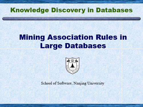
Chapter 6. Mining Association Rules in Large Databases
关联规则

剪 枝
由Lk-1生成Ck, 所有Lk都在Ck中,但Ck可能仍 然很大,需要对Ck进行剪枝,再使Ck减小, 得到最后的候选集。剪枝过程如下: 再判断Ck中k-1子项目集是否在Lk-1中,如不 在,那么这个Ck就不会是频繁项目集。从Ck 删除。 Ck就会大大减小。 由{i1, i3 ,i4 ,i6} ,{i1, i3 ,i4 ,i8}产生的{i1, i3 ,i4 ,i6, ,i8} 如{ i3 ,i4 ,i6, ,i8}或 {i1,,i4 ,i6, ,i8}……不在Lk-1中, {i1, i3 ,i4 ,i6, ,i8}就应删去。
22
Apriori 算法说明
例子:最小支持度设为2。 D(数据库) C1 (候选集)
TID T100 T200 T300 T400 T500 T600 T700 T800 T900 D中的项目 i1 i2 i2 i1 i1 i2 i1 i1 i1 i2 i5 i4 i3 i2 i4 i3 i3 i3 i2 i3 i5 i2 i3 项集 支持度 {i 1 } {i 2 } {i 3 } {i 4 } {i 5 } 6 7 6 2 2
10
3、若有事务T,其中 X T, Y T, X∩Y=, X∪Y T, X、Y也为项目集;则形如 XY 的规则称为关联规则;(即购物事务,购买X, 也购买Y); 4、在数据库D中,若s% 的事务包含X∪Y,则关联 规则XY的支持率为s%;在数据库 D 中,若c% 包含项目集X的事务的也包含项目集Y,则关联 规则XY的置信度为c%。
13
关联规则挖掘分为两步:
1、找频繁(大)项目集 大于最小支持度项集 2、找强关联规则 大于最小支持度和最小置信度的关联规则
第二个任务已经圆满解决。关联规则挖掘的研 究工作多为找频繁集的各种算法。
Association_Rule

Support: 2/8
Confidence: 1/3
Milk Bread
Support: 2/8 Confidence: 2/3
Frequent Itemsets and Strong Rules
Support and Confidence are bounded by thresholds:
C3 {{1, 2,3}}
24
Lk Ck+1
{X Yk | X , Y Lk , X i Yi , i [1, k 1], X k Yk }
Ordered List
L2 {{1, 2},{2,3}} L2 {{1,3},{2,3}} L2 {{1, 2},{1,3},{2,3}} L2 {{1, 2},{1,3}}
Searching for rules in the form of: Bread Butter
6
7
Support of an Itemset
Itemset
Bread
Butter Chips Jelly
Support
6/8
3/8 2/8 3/8
Itemset
Bread, Butter
Support
Minimum support σ
Minimum confidence Φ A frequent (large) itemset is an itemset with support larger than σ. A strong rule is a rule that is frequent and its confidence is higher than Φ. Association Rule Problem Given I, D, σ and Φ, to find all strong rules in the form of XY. The number of all possible association rules is huge. Brute force strategy is infeasible. A smart way is to find frequent itemsets first.
大学英语学术写作参考答案人大版

Exercise 2
Introduction 1
民
人 S5—S3—S1—S6—S8—S2—S7—S9—S4
人 4. It’s not good to ask the question which yields a “yes” or “no” answer. A good question may be “To what extent do adolescents believe that their peers have favorable views of cosplay?”. 5. Of the four questions, the second is obviously more general. One way to solve this problem is
大 school, and how are these commonalities used to aid the school doctors to prevent sports
injuries?”. 3. The topic is so broad in nature, that even a book would not be sufficient to answer the question.
中Research questions: 1) In what ways have the parents influenced their children’s puppy love? 2) How did the parents respond to their children’s puppy love? 3) How was the parent-child relationship affected by puppy love?
Apriori

MLA Group
Apriori
Item sup K=1 { A} { B} C1 {C} support<50 { D} { E} 50% 75% 75% 25% 75%
L2
{ A,C} { B,C} { B,E} { C,E}
50% 50% 75% 50%
L1
{A} {B} {C} {E}
50% 75% 75% 75%
A Brief Introduction to Apriori
2
MLA Group
Outline
What is Association Rules? Apriori Algorithms Challenge of Apriori
A Brief Introduction to MIL
3
MLA Group
K=2
C2
Item sup support<50 { A,B } 25% { A,C} 50% support<50 25% {A,E} { B,C} 50% { B,E} 75% { C,E} 50%
A Brief Introduction to Apriori
MLA Group
Apriori
L2 { A,C} { B,C} { B,E} { C,E} 50% 50% 75% 50%
MLA Group
Apriori
Apriori is a classic algorithm for learning association rules posted by R.Agrawal and R.Srikant in 1994. The purpose of the Apriori Algorithm is to find associations between different sets of data Rakesh Agrawal and Ramakrishnan Srikant. Fast algorithms for mining association rules in large databases. Proceedings of the 20th International Conference on Very Large Data Bases, VLDB, pages 487-499, Santiago, Chile, September 1994.
1. Data Mining – Practical Machine Learning Tools and Techniques with Java
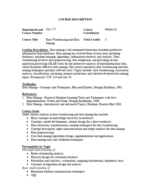
COURSE DESCRIPTIONDepartment and Course Number CSc 177 CourseCoordinatorMeiliu LuCourse Title Data Warehousing and DataMiningTotal Credits 3Catalog Description: Data mining is the automated extraction of hidden predictive information from databases. Data mining has evolved from several areas including: databases, machine learning, algorithms, information retrieval, and statistics. Data warehousing involves data preprocessing, data integration, and providing on-line analytical processing (OLAP) tools for the interactive analysis of multidimensional data, which facilitates effective data mining. This course introduces data warehousing and data mining techniques and their software tools. Topics include: data warehousing, association analysis, classification, clustering, numeric prediction, and selected advanced data mining topics. Prerequisite: CSC 134 and Stat 50.Textbooks:Data Mining – Concepts and Techniques, Han and Kamber, Morgan Kaufman, 2001.References:1.Data Mining – Practical Machine Learning Tools and Techniques with JavaImplementation, Witten and Frank, Morgan Kaufmann, 2000;2.Data Mining – Introductory and Advanced Topics, Dunham, Prentice Hall 2003.Course GoalsStudy various subjects in data warehousing and data mining that include: •Basic concepts on knowledge discovery in databases•Concepts, model development, schema design for a data warehouse•Data extraction, transformation, loading techniques for data warehousing•Concept description: input characterization and output analysis for data mining •Data preprocessing•Core data mining algorithms design, implementation and applications•Data mining tools and validation techniquesPrerequisites by TopicThorough understanding of:•Entity-relationship analysis•Physical design of a relational database•Probability and statistics – estimation, sampling distributions, hypothesis tests •Concepts of algorithm design and analysisBasic understanding of:•Relational database normalization techniques•SQLExposure to:•Bayesian theory•RegressionMajor Topics Covered in the Course1.Introduction to the process of knowledge discovery in databases2.Basic concepts of data warehousing and data mining3.Data preprocessing techniques: selection, extraction, transformation, loading4.Data warehouse design and implementation: multidimensional data model, casestudy using Oracle technology5.Machine learning schemes in data mining: finding and describing structure patterns(models) in data, informing future decisionsrmation theory and statistics in data mining: from entropy to regression7.Data mining core algorithms: statistical modeling, classification, clustering,association analysis8.Credibility: evaluating what has been leaned from training data and predictingmodel performance on new data, evaluation methods, and evaluation metrics9.Weka: a set of commonly used machine learning algorithms implemented in Javafor data mining10.C5 and Cubist: Decision tree and model tree based data mining tools11.Selected advance topics based on students’ interests such as: web mining, textmining, statistical learning12.Case studies of real data mining applications (paper survey and invited speaker) Laboratory Projects1.Design and implement a data warehouse database (4 weeks)2.Explore extraction, transformation, loading tasks in data warehousing (1 week)3.Explore data mining tools and algorithms implementation (3 weeks)4.Design and implement data mining application (3 weeks)Expected OutcomesThorough understanding of:•Process and tasks for Knowledge discovery in databases.•Differences between a data warehouses OLAP and operational databases OLTP.•Multidimensional data model design and development.•Techniques for data extraction, transformation, and loading.•Machine learning schemes in data mining.•Mining association rules (Apriori).•Classification and prediction (Statistical based: Naïve Bayes, regression trees and model trees; Distance based: KNN, Decision tree based: 1R, ID3, CART;Covering algorithm: Prism).•Cluster analysis (Hierarchical algorithms: single link, average link, and complete link; Partitional algorithms: MST, K-means; Probability based algorithm: EM).•Use of data mining tools: C5, Cubist, Weka.Basic understanding of:•Data warehouse architecture.•Information theory and statistics in data mining.•Credibility analysis and performance evaluation.Exposure to:•Mining complex types of data: multimedia, spatial, and temporal•Statistical learning theory•Support vector machine and ANNEstimated CSAB Category ContentCORE ADVANCED CORE ADVANCEDDataStructures .2Algorithms 1 Computer Org & ArchitectureSoftwareDesign .5 Concepts ofProgrammingLanguages .2Oral and Written Communications1.Three written reports (term project proposal, research paper review, and termproject report).2.Two oral presentations (10 minutes for paper review and 15-20 minutes for termproject).Social and Ethical IssuesNo significant component.Theoretical Content1.Data warehouse schema and data cube computation.rmation theory and statistics in data mining.3.Data mining algorithms and their output model performance prediction.4.Evaluation metrics (confusion matrix, cost matrix, F measure, ROC curve). Analysis and Design1.Design of a data warehouse.2.Design of a process of ETL (Extraction, Transformation, Loading).3.Design of a data mining application.4.Analysis of performance of a data warehouse.5.Analysis and comparison of data mining schema.CSC 17711-04。
第五章_关联规则挖掘
Any subset of a frequent itemset must be frequent
Mining Frequent Itemsets: the Key Step
Find the frequent itemsets: the sets of
items that have minimum support A subset of a frequent itemset must also be a frequent itemset
Customer buys diaper
Find all the rules X & Y Z
with minimum confidence and support
support, s, probability that a transaction contains {X , Y , Z}
Customer buys beer
Use the frequent itemsets to generate association rules.
The Apriori Algorithm
Join Step: Ck is generated by joining Lk-1with itself Prune Step: Any (k-1)-itemset that is not frequent cannot be a subset of a frequent k-itemset
[0.2%, 60%] age(x, “30..39”) ^ income(x, “42..48K”) buys(x, “PC”) [1%, 75%] Single dimension vs. multiple dimensional associations (see ex. Above) Single level vs. multiple-level analysis What brands of beers are associated with what brands of diapers? Various extensions Correlation, causality analysis
产品全生命周期价值计量与决策
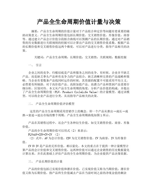
产品全生命周期价值计量与决策摘要:产品全生命周期的价值计量对于产品组合和定价等问题有着重要的辅助决策意义。
产品全生命周期价值包括长期价值,交叉销售价值,形象价值,商誉等。
通过建立产品会计价值分段拟合曲线可以预测产品的长期价值;通过对产品销售的历史数据进行关联规则的挖掘可以计算出产品的交叉销售价值系数。
根据产品的长期价值和交叉销售价值这两个维度,可以对产品进行分类,指导产品相关的决策。
关键词:产品全生命周期;长期价值;交叉销售;关联规则;数据挖掘一、引言企业之间的竞争,归根结底是产品和服务之间的竞争。
有时候,企业并不缺乏产品,而是缺乏拳头产品和有竞争力的产品组合,缺乏清晰和完善的产品战略和策略。
当企业有着数条产品线同时运作的时候,其资源的配置不可能采用平均主义,必然要有所倾斜,对于高价值产品、高附加值产品、高潜力产品和黑洞产品需要仔细分析,区别对待。
本文从产品全生命周期的角度,分析产品价值的构成,并提出了产品全生命周期价值(PLV,Product CycleLife Value)的计量模型,通过该模型,可以将企业产品进行分类,从而指导产品相关的决策。
二、产品全生命周期价值评估模型这里的产品全生命周期采用营销学上的概念,即一个产品从推出→成长→成熟→衰退→退出市场的整个周期。
产品全生命周期曲线如图1所示。
产品在其销售过程中,还会产生各种衍生价值,如交叉销售价值,商誉,形象价值。
产品的全生命周期价值可以用式(2)来表示:PLV=AV+CSV+CV+IV (2)(2)式中,AV为会计价值,CSV为交叉销售价值,CV为商誉,IV为形象价值。
CV和IV是产品的无形价值,难以量化。
本文的重点在于提供一种计量模型计算产品的会计价值和交叉销售价值,这两种价值可以通过企业销售的历史数据量化计算出来,并在此基础上评估产品的全生命周期价值,为企业提供产品决策依据。
三、产品长期价值的计量产品的价值包括已实现价值和潜在价值,已实现价值又称为当期价值;潜在价值又称为长期价值,指产品终生价值减去产品在当前时刻之前的净现金值的剩余值,可以采用分段函数来拟合产品的长期价值曲线。
关联规则挖掘综述
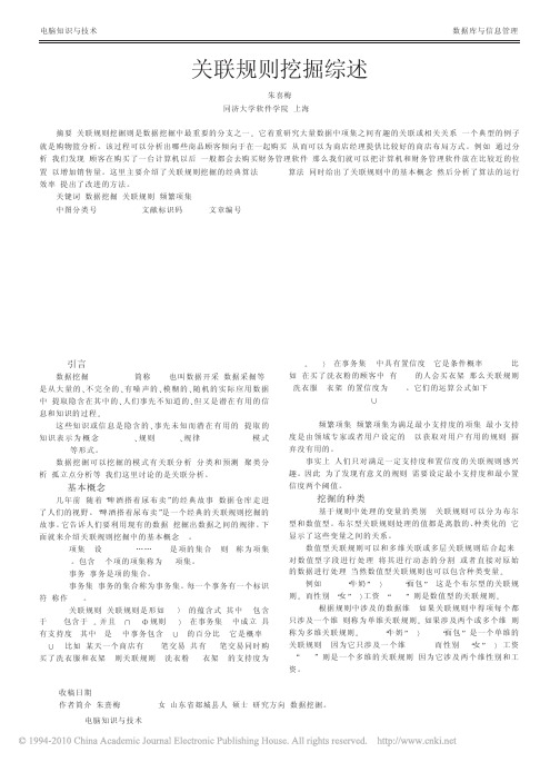
5.1 算法的基本思想: Apriori 算法主要工作在于寻找频繁项集。通过先计算所有的 候选 1- 项集的集合 C1。找出所有的频繁 1- 项集 L1。然后根据频 繁 1- 项集 L1 确定候选 2- 项集的集合 C2。从 C2 中找出所有的频 繁 2- 项 集 L2。 再 根 据 频 繁 2- 项 集 L2 确 定 候 选 3- 项 集 的 集 合 C3。从 C3 中找出所有的频繁 3- 项集 L3。如此下去直到不再有候 选项集。算法 Apriori: L1=find_frequent_1- itemsets(D); for(k=2;LK- 1! =NULL;K++) {Ck=aprori_gen(Lk- 1); //由 Lk- 1 经过连接和剪枝产生 K 候选项集 for each transaction t∈D //扫 描 所 有 的 事 务 {Ct=subset(Ck,t); //从 t 中取得是候选集的子集 for each candidate c∈Ct c.count++;} Lk={c∈Ck|c.count>=min_sup} }Return L=UkLk; 在 论 文 中 , Agrawal 等 引 入 了 修 剪 技 术 ( Pruning) 来 减 小 候 选 集 Ck 的大小, 利用我们前面介绍过得性质: 频繁项集的所有非空 子集都必须也是频繁的。 这个修剪过程可以降低计算所有的候选集的支持度的代价。 在论文[1]中, 还引入了杂凑树( Hash Tree) 方法来有效的计算每个 项集的支持度。 5.2 算法的性能分析 在 apriori 算 法 中 , Ck 中 的 每 个 元 素 需 要 在 交 易 数 据 库 中 进 行验证以决定是否加入 Lk, 它可能需要重复地扫描事务数据库, 这里的验证过程是算法性能的一个瓶颈。当数据库很大的时候, 就会需要很大的 I/O 负载。 5.3 算法的改进 虽然 aprori 算法自身提供了一些改进, 但是仍然不能令人满 意, 所以人们提出了很多解决的方案, 旨在提高原算法的效率。涉 及 散 列 和 事 务 压 缩 的 变 形 可 以 用 来 使 得 过 程 变 得 更 有 效 。其 他 变 形涉及划分数据( 在每一部分上挖掘, 然后合并结果) 和数据选样 ( 在数据子集上挖掘) 。这些变形可以将数据扫描次数减少到两次
R-Agrawalg关于关联规则的开创性论文
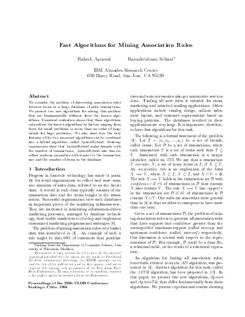
X =) Y , where X I, Y I, and X \ Y = .
The rule X =) Y holds in the transaction set D with
con dence c if c% of transactions in D that contain
X also contain Y . The rule X =) Y has support s
An algorithm for nding all association rules, henceforth referred to as the AIS algorithm, was presented in 4]. Another algorithm for this task, called the SETM algorithm, has been proposed in 13]. In this paper, we present two new algorithms, Apriori and AprioriTid, that di er fundamentally from these algorithms. We present experimental results showing
PSarnotcieaegdoi,nCgshoilfe,th1e99240th VLDB Conference
tires and auto accessories also get automotive services done. Finding all such rules is valuable for crossmarketing and attached mailing applications. Other applications include catalog design, add-on sales, store layout, and customer segmentation based on buying patterns. The databases involved in these applications are very large. It is imperative, therefore, to have fast algorithms for this task.
关联规则挖掘AssociationRuleMining背景简介

Brute-force approach:
– List all possible association rules – Compute the support and confidence for each rule – Prune rules that fail the minsup and minconf thresholds Computationally prohibitive!
Apriori principle:
– If an itemset is frequent, then all of its subsets must also be frequent
Apriori principle holds due to the following property of the support measure:
TID Items
– k-itemset
An itemset that contains k items
1 2 3 4 5
Bread, Milk Bread, Diaper, Beer, Eggs Milk, Diaper, Beer, Coke Bread, Milk, Diaper, Beer Bread, Milk, Diaper, Coke
Frequent Itemset Generation
null
A
B
C
D
E
AB
AC
AD
AE
BC
BD
BE
CD
CE
DE
关联分析

务中出现的频繁程度
2 0.4 5
(Milk, Diaper, Beer ) 2 c 0.67 (Milk , Diaper ) 3
关联规则挖掘问题
关联规则挖掘问题:给定事务的集合 T, 关联规则 发现是指找出支持度大于等于 minsup并且置信度 大于等于minconf的所有规则, minsup和minconf是 对应的支持度和置信度阈值 挖掘关联规则的一种原始方法是:Brute-force approach:
List of Candidates
N
M
w
– 时间复杂度 ~ O(NMw),这种方法的开销可能非常大。
降低产生频繁项集计算复杂度的方法
减少候选项集的数量 (M)
– 先验(apriori)原理
减少比较的次数 (NM)
– 替代将每个候选项集与每个事务相匹配,可以使用更高 级的数据结构,或存储候选项集或压缩数据集,来减少 比较次数
候选的产生与剪枝
候选的产生与剪枝
– 避免产生重复的候选项集的一种方法是确保每 个频繁项集中的项以字典序存储,每个频繁( k-1)-项集X只用字典序比X中所有的项都大的 频繁项进行扩展 如:项集{面包,尿布}可以用项集{牛奶}扩展, 因为“牛奶”(milk)在字典序下比“面包” (Bread)和“尿布”(Diapers)都大。 – 尽管这种方法比蛮力方法有明显改进,但是仍 然产生大量不必要的候选。 例如,通过合并{啤酒,尿布}和{牛奶}而得到的 候选是不必要的。因为它的子集{啤酒,牛奶} 是非频繁的。
候选的产生与剪枝
Fk 1 Fk 1方法
– 这种方法合并一对频繁(k-1)-项集,仅当它们的前k2个项都相同。 如频繁项集{面包,尿布}和{面包,牛奶}合并,形成了 候选3-项集{面包,尿布,牛奶}。算法不会合并项集{啤 酒,尿布}和{尿布,牛奶},因为它们的第一个项不相 同。 – 然而,由于每个候选都由一对频繁(k-1)-项集合并而 成,因此,需要附加的候选剪枝步骤来确保该候选的 其余k-2个子集是频繁的。
On the Complexity ofMiningQuantitative Association Rules
which may be denoted:
Toothbrush :
Editor: Raymond Ng, Jiawei Han, and Laks Lakshmanan
interesting and important research problem. Recently, di erent aspects of the problem have been studied, and several algorithms have been presented in the literature, among others in (Srikant and Agrawal, 1996 Fukuda et al., 1996a Fukuda et al., 1996b Yoda et al., 1997 Miller and Yang, 1997). An aspect of the problem that has so far been ignored, is its computational complexity. In this paper, we study the computational complexity of mining quantitative association rules.
Pleinlaan 2, gebouw G-10, B-1050 Brussel Phone: +32-2-629.3308 • Fax: +32-2-629.3525
关联规则挖掘算法综述

关联规则挖掘算法综述本文介绍了关联规则的基本概念和分类方法, 列举了一些关联规则挖掘算法并简 要分析了典型算法,展望了关联规则挖掘的未来研究方向。
1 引言关联规则挖掘发现大量数据中项集之间有趣的关联或相关联系。
它在数据挖掘中 是一个重要的课题,最近几年已被业界所广泛研究。
关联规则挖掘的一个典型例子是购物篮分析。
关联规则研究有助于发现交易数据 库中不同商品(项)之间的联系,找出顾客购买行为模式,如购买了某一商品对 购买其他商品的影响。
分析结果可以应用于商品货架布局、货存安排以及根据购 买模式对用户进行分类。
Agrawal 等于 1993 年首先提出了挖掘顾客交易数据库中项集间的关联规则问题 [AIS93b],以后诸多的研究人员对关联规则的挖掘问题进行了大量的研究。
他们 的工作包括对原有的算法进行优化,如引入随机采样、并行的思想等,以提高算 法挖掘规则的效率;对关联规则的应用进行推广。
最近也有独立于 Agrawal 的频集方法的工作[HPY00],以避免频集方法的一些缺 陷,探索挖掘关联规则的新方法。
也有一些工作[KPR98]注重于对挖掘到的模式 的价值进行评估,他们提出的模型建议了一些值得考虑的研究方向。
2 基本概念设 I={i1,i2,..,im}是项集,其中 ik(k=1,2,…,m)可以是购物篮中的物品,也可 以是保险公司的顾客。
设任务相关的数据 D 是事务集,其中每个事务 T 是项集, 使得 TÍI。
设 A 是一个项集,且 AÍT。
关联规则是如下形式的逻辑蕴涵:A Þ B,AÌI, AÌI,且 A∩B=F。
关联规则具有如下两个重要的属性: 支持度: P(A∪B),即 A 和 B 这两个项集在事务集 D 中同时出现的概率。
置信度: P(B|A),即在出现项集 A 的事务集 D 中,项集 B 也同时出现的概率。
IEEE TRANSACTIONS ON KNOWLEDGE AND DATA ENGINEERING 1 A Transaction Mapping Algorithm for F
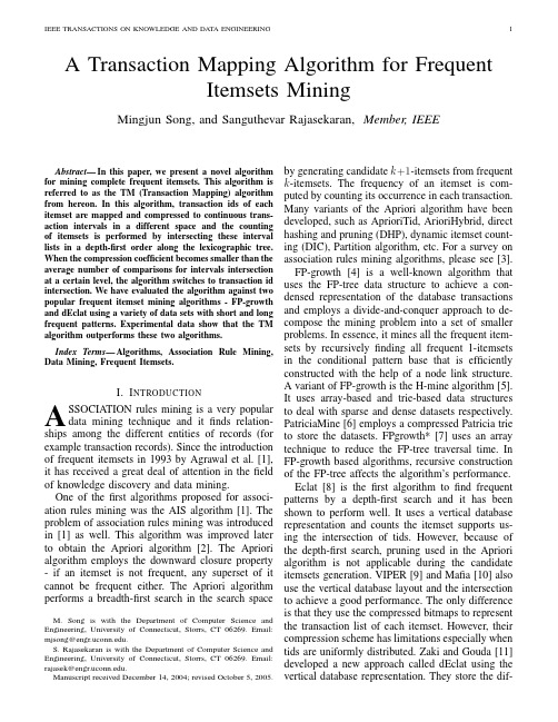
A Transaction Mapping Algorithm for FrequentItemsets MiningMingjun Song,and Sanguthevar Rajasekaran,Member,IEEEAbstract—In this paper,we present a novel algorithm for mining complete frequent itemsets.This algorithm is referred to as the TM(Transaction Mapping)algorithm from hereon.In this algorithm,transaction ids of each itemset are mapped and compressed to continuous trans-action intervals in a different space and the counting of itemsets is performed by intersecting these interval lists in a depth-first order along the lexicographic tree. When the compression coefficient becomes smaller than the average number of comparisons for intervals intersection at a certain level,the algorithm switches to transaction id intersection.We have evaluated the algorithm against two popular frequent itemset mining algorithms-FP-growth and dEclat using a variety of data sets with short and long frequent patterns.Experimental data show that the TM algorithm outperforms these two algorithms.Index Terms—Algorithms,Association Rule Mining, Data Mining,Frequent Itemsets.I.I NTRODUCTIONA SSOCIATION rules mining is a very populardata mining technique and itfinds relation-ships among the different entities of records(for example transaction records).Since the introduction of frequent itemsets in1993by Agrawal et al.[1], it has received a great deal of attention in thefield of knowledge discovery and data mining.One of thefirst algorithms proposed for associ-ation rules mining was the AIS algorithm[1].The problem of association rules mining was introduced in[1]as well.This algorithm was improved later to obtain the Apriori algorithm[2].The Apriori algorithm employs the downward closure property -if an itemset is not frequent,any superset of it cannot be frequent either.The Apriori algorithm performs a breadth-first search in the search space M.Song is with the Department of Computer Science and Engineering,University of Connecticut,Storrs,CT06269.Email: mjsong@.S.Rajasekaran is with the Department of Computer Science and Engineering,University of Connecticut,Storrs,CT06269.Email: rajasek@.Manuscript received December14,2004;revised October5,2005.by generating candidate k+1-itemsets from frequent k-itemsets.The frequency of an itemset is com-puted by counting its occurrence in each transaction. Many variants of the Apriori algorithm have been developed,such as AprioriTid,ArioriHybrid,direct hashing and pruning(DHP),dynamic itemset count-ing(DIC),Partition algorithm,etc.For a survey on association rules mining algorithms,please see[3]. FP-growth[4]is a well-known algorithm that uses the FP-tree data structure to achieve a con-densed representation of the database transactions and employs a divide-and-conquer approach to de-compose the mining problem into a set of smaller problems.In essence,it mines all the frequent item-sets by recursivelyfinding all frequent1-itemsets in the conditional pattern base that is efficiently constructed with the help of a node link structure.A variant of FP-growth is the H-mine algorithm[5]. It uses array-based and trie-based data structures to deal with sparse and dense datasets respectively. PatriciaMine[6]employs a compressed Patricia trie to store the datasets.FPgrowth*[7]uses an array technique to reduce the FP-tree traversal time.In FP-growth based algorithms,recursive construction of the FP-tree affects the algorithm’s performance. Eclat[8]is thefirst algorithm tofind frequent patterns by a depth-first search and it has been shown to perform well.It uses a vertical database representation and counts the itemset supports us-ing the intersection of tids.However,because of the depth-first search,pruning used in the Apriori algorithm is not applicable during the candidate itemsets generation.VIPER[9]and Mafia[10]also use the vertical database layout and the intersection to achieve a good performance.The only difference is that they use the compressed bitmaps to represent the transaction list of each itemset.However,their compression scheme has limitations especially when tids are uniformly distributed.Zaki and Gouda[11] developed a new approach called dEclat using the vertical database representation.They store the dif-ference of tids called diffset between a candidate k-itemset and its prefix k−1-frequent itemsets,instead of the tids intersection set,denoted here as tidset. They compute the support by subtracting the cardi-nality of diffset from the support of its prefix k−1-frequent itemset.This algorithm has been shown to gain significant performance improvements over Eclat.However,when the database is sparse,diffset will lose its advantage over tidset.In this paper,we present a novel approach that maps and compresses the transaction id list of each itemset into an interval list using a transaction tree, and counts the support of each itemset by intersect-ing these interval lists.The frequent itemsets are found in a depth-first order along a lexicographic tree as done in the Eclat algorithm.The basic idea is to save the intersection time in Eclat by mapping transaction ids into continuous transaction intervals. When these intervals become scattered,we switch to transaction ids as in Eclat.We call the new algorithm the TM(transaction mapping)algorithm. The rest of the paper is arranged as follows:section II introduces the basic concept of association rules mining,two types of data representation,and the lexicographic tree used in our algorithm;section III addresses how the transaction id list of each itemset is compressed to a continuous interval list,and the details of the TM algorithm;section IV gives an analysis of the compression efficiency of transaction mapping;section V experimentally compares the TM algorithm with two popular algorithms-FP-Growth and dEclat;in section VI,we provide some general comments;section VII concludes the paper.II.BASIC PRINCIPLESA.Association Rules MiningLet I={i1,i2,...,i m}be a set of items and let D be a database having a set of transactions where each transaction T is a subset of I.An association rule is an association relationship of the form:X⇒Y,where X⊂I,Y⊂I,and X∩Y=∅.The support of rule X⇒Y is defined as the percentage of transactions containing both X and Y in D.The confidence of X⇒Y is defined as the percentage of transactions containing X that also contain Y in D.The task of association rules mining is tofind all strong association rules that satisfy a minimum support threshold(min sup)and a minimum confidence threshold(min conf).MiningTABLE IH ORIZONTAL REPRESENTATIONtid items12,1,5,322,331,443,1,552,1,362,4TABLE IIV ERTICAL TIDSET REPRESENTATIONitem tidset11,3,4,521,2,5,631,2,4,54351,4association rules consists of two phases.In thefirst phase,all frequent itemsets that satisfy the min sup are found.In the second phase,strong association rules are generated from the frequent itemsets found in thefirst phase.Most research considers only the first phase because once frequent itemsets are found, mining association rules is trivial.B.Data RepresentationTwo types of database layouts are employed in association rules mining:horizontal and vertical. In the traditional horizontal database layout,each transaction consists of a set of items and the data-base contains a set of transactions.Most Apriori-like algorithms use this type of layout.For vertical data-base layout,each item maintains a set of transaction ids(denoted by tidset)where this item is contained. This layout could be maintained as a bitvector.Eclat uses tidsets while VIPER and Mafia use compressed bitvectors.It has been shown that vertical layout performs generally better than horizontal format[8] [9].Tables I through III show examples for different types of layouts.C.Lexicographic Prefix TreeIn this paper,we employ a lexicographic prefix tree data structure to efficiently generate candidate itemsets and count their frequency,which is verySONG AND RAJASEKARAN:A TRANSACTION MAPPING ALGORITHM FOR FREQUENT ITEMSETS MINING3TABLE IIIV ERTICAL BITVECTOR REPRESENTATIONitem bitvector11011102110011311011040010005100100similar to the lexicographic tree used in the TreeP-rojection algorithm[12].This tree structure is also used in many other algorithms such as Eclat[8]. An example of this tree is shown in Fig.1.Each node in the tree stores a collection of frequent itemsets together with the support of these itemsets. The root contains all frequent1-itemsets.Itemsets in level l(for any l)are frequent l-itemsets.Each edge in the tree is labeled with an item.Itemsets in any node are stored as singleton sets with the understanding that the actual itemset also contains all the items found on the edges from this node to the root.For example,consider the leftmost node in level2of the tree in Fig.1.There are four2-itemsets in this node,namely,{1,2},{1,3},{1,4}, and{1,5}.The singleton sets in each node of the tree are stored in the lexicographic order.If the root contains{1},{2},...,{n},then,the nodes in level 2will contain{2},{3},...,{n};{3},{4},...,{n}; ...;{n},and so on.For each candidate itemset, we also store a list of transaction ids(i.e.,ids of transactions in which all the items of the itemset occur).This tree will not be generated in full.The tree is generated in a depthfirst order and at any given time,we only store minimum information needed to continue the search.In particular,this means that at any instance at most a path of the tree will be stored.As the search progresses,if the expansion of a node cannot possibly lead to the discovery of itemsets that have minimum support, then the node will not be expanded and the search will backtrack.As a frequent itemset that meets the minimum support requirement is found,it is output. Candidate itemsets generated by depthfirst search are the same as those generated by thejoining step (without pruning)of the Apriori algorithm.Fig.1.Illustration of lexicographic treeIII.TM ALGORITHMOur contribution is that we compress tids(trans-action ids)for each itemset to continuous intervals by mapping transaction ids into a different space appealing to a transaction tree.Thefinding of fre-quent itemsets is done by intersecting these interval lists instead of intersecting the transaction id lists (as in the Eclat algorithm).We will begin with the construction of a transaction tree.A.Transaction treeThe transaction tree is similar to FP-tree except that there is no header table or node link.The transaction tree can be thought of as a compact representation of all the transactions in the database. Each node in the tree has an id corresponding to an item and a counter that keeps the number of transactions that contain this item in this path. Adapted from[4],the construction of the transaction tree(called construcTransactionTree)is as follows: 1)Scan through the database once and identify all the frequent1-itemsets and sort them in descending order of frequency.At the beginning the transaction tree consists of just a single node(which is a dummy root).2)Scan through the database for a second time. For each transaction,select items that are in frequent 1-itemsets,sort them according to the order of fre-quent1-itemsets and insert them into the transaction tree.When inserting an item,start from the root. At the beginning the root is the current node.In4IEEE TRANSACTIONS ON KNOWLEDGE AND DATA ENGINEERINGTABLE IVA SAMPLE TRANSACTION DATABASETID Items Ordered frequent items12,1,5,3,19,201,2,322,6,32,331,7,8143,1,9,101,352,1,11,3,17,181,2,362,4,122,471,13,14182,15,4,162,4Fig.2.A transaction tree for the above databasegeneral,if the current node has a child node whose id is equal to this item,then just increment the count of this child by1,otherwise create a new child node and set its counter as1.Table IV and Fig.2illustrate the construction of a transaction tree.Table IV shows an example of a transaction database and Fig.2displays the constructed transaction tree assuming the minimum support count is2.The number before the colon in each node is the item id and the number after the colon is the count of this item in this path.B.Transaction mapping and the construction of interval listsAfter the transaction tree is constructed,all the transactions that contain an item are represented with an interval list.Each interval corresponds to a contiguous sequence of relabeled ids.Each node in the transaction tree will be associated with an inter-val.The construction of interval lists for each itemTABLE VE XAMPLE OF TRANSACTION MAPPINGItem Mapped transaction interval list1[1,500]2[1,200],[501,800]3[1,300],[501,600]4[601,800]is done recursively starting from the root in a depth-first order.The process is described as follows:Consider a node u whose number of transactionsis c and whose associated interval is[s,e].Heres is the relabeled start id and e is the relabeled end id with e−s+1=c.Assume that u hasm children with child i having c i transactions,fori=1,2,...,m.It is obvious that m i=1c i≤c.If the intervals associated with the children of u are:[s1,e1],[s2,e2],...,[s m,e m],these intervals areconstructed as follows:s1=s(1)e1=s1+c1−1(2) s i=e i−1+1,for i=2,3,...,m(3)e i=s i+c i−1,for i=2,3,...,m(4) For the root,s=1.For example,in Fig.2,the root has two children.For thefirst child,s1=1,e1= 1+5−1=5,so the interval is[1,5];for the second child,s2=5+1=6,e2=6+3−1=8, so the interval is[6,8].The compressed transaction id lists of each item is ordered by the start id of each associated interval.In addition,if two intervals are contiguous,they will be merged and replaced with a single interval.For example,each interval associated with each node is shown in Fig.2.Two intervals of item3,[1,2]and[3,3]will be merged to[1,3].To illustrate the efficiency of this mappingprocess more clearly,assume that the eight trans-actions of the example database shown in table IVrepeat100times each.In this case the transactiontree becomes the one shown in Fig.3.The mapped transaction interval lists for eachitem is shown in Table V,where1-300of item3results from the merging of1-200and201-300. We now summarize a procedure(called map-TransactionIntervals)that computes the interval lists for each item as follows:Using depthfirst order,SONG AND RAJASEKARAN:A TRANSACTION MAPPING ALGORITHM FOR FREQUENT ITEMSETS MINING5Fig.3.Transaction tree for illustrationtraverse the transaction tree.For each node,create an interval composed of a start id and an end id.If it is the first child of its parent,then the start id of the interval is equal to the start id of the parent (equation (1))and the end id is computed by equation (2).If not,the start id is computed by equation (3),and the end id is computed by equation (4).Insert this interval to the interval list of the corresponding item.Once the interval lists for frequent 1-itemsets are constructed,frequent i -itemsets (for any i )are found by intersecting interval lists along the lexicograpgic tree.Details are provided in the next subsection.C.Interval lists intersectionIn addition to the items described above,each element of a node in the lexicographic tree also stores a transaction interval list (corresponding to the itemset denoted by the element).By constructing the lexicographic tree in a depth-first order,the support count of the candidate itemset is computed by intersecting the interval lists of the two elements.For example,element 2in the second level of the lexicographic tree in Fig.1represents the itemset 1,2,whose support count is computed by intersect-ing the interval lists of itemset 1and itemset 2.In contrast,Eclat uses a tid list intersection.Intervallists intersection is more efficient.Note that since the interval is constructed from the transaction tree,it cannot partially contain or be partially contained in another interval.There are only three possiblerelationships between any two intervals A =[s 1,e 1]and B =[s 2,e 2].1)A ∩B =∅.In this case,interval A and interval B come from different paths of the transaction tree.For instance,interval [1,500]and interval [501,800]in table V.2)A ⊇B .In this case,interval A comes from the ancestor nodes of interval B in the transaction tree.For instance,interval [1,500]and interval [1,300]in table V.3)A ⊆B .In this case,interval A comes from the descendant nodes of interval B in the transaction tree.For instance,interval [1,300]and interval [1,500]in table V.Considering the above three cases,the average number of comparisons for two intervals is 2.D.SwitchingAfter a certain level of the lexicographic tree,the transaction interval lists of elements in any node will be expected to become scattered.There could be many transaction intervals that contain only single tids.At this point,interval representation will lose its advantage over single tid represen-tation,because the intersection of two segments will use three comparisons in the worst case while the intersection of two single tids only needs one comparison.Therefore,we need to switch to the single tid representation at some point.Here,we define a coefficient of compression for one node inthe lexicographic tree,denoted by coeff ,as follows:Assume that a node has m elements,and let s i rep-resent the support of the i th element,l i representing the size of the transaction list of the i th element.Then,coeff =1m mi =1s i l iFor the intersection of two interval lists,the average number of comparisons is 2,so we will switch to tid set intersection when coeff is less than 2.E.Details of the TM AlgorithmNow we provide details on the steps involved in the TM algorithm.There are four steps involved:1)Scan through the database and identify all frequent-1itemsets.2)Construct the transaction tree with counts for each node.3)Construct the transaction interval lists.Merge intervals if they are mergeable (i.e.,if the intervals are contiguous).6IEEE TRANSACTIONS ON KNOWLEDGE AND DATAENGINEERINGFig.4.Full transaction tree4)Construct the lexicographic tree in a depth first order keeping only the minimum amount of information necessary to complete the search.This in particular means that no more than a path in the lexicographic tree will ever be stored.While at any node,if further expansion of that will not be fruitful,then the search backtracks.When process-ing a node in the tree,for every element in the node,the corresponding interval lists are computed by interval intersections.As the search progresses,itemsets with enough support are output.When the compression coefficient of a node becomes less than 2,switch to tid list intersection.In the next section we provide an analysis to indi-cate how TM can provide computational effiPRESSION AND TIME ANALYSISOF TRANSACTION MAPPINGSuppose the transaction tree is fully filled in the worst case as illustrated in Fig.4,where the sub-script of C is the possible itemset,and C represents the count for this itemset.Assume that there are n frequent 1-itemsets with a support of S 1,S 2,...,S n respectively.Then we have the following relationships:S 1=C 1=|T 1|S 2=C 2+C 1,2=|T 1|+|T 1,2|S 3=C 3+C 1,3+C 1,2,3+C 2,3=|T 3|+|T 1,3|+|T 1,2,3|+|T 2,3|...S n =C n +C 1,n +C 2,n +...+C n −1,n +C 1,2,n+C 1,3,n +...=|T n |+|T 1,n |+|T 2,n |+...+|T n −1,n |+|T 1,2,n |+|T 1,3,n |+...Here each T represents the interval for a node,and |T |represents the length of T ,which is equal to C .The maximum number of intervals possible for each frequent 1-itemset i is 2i −1.The average compression ratio is Avg ratio ≥S 1+S 221+S 322+...+S i 2i −1+...+S n 2n −1≥S n (1+121+122+...+12n −1)=2S n (1−2−n )When S n ,which is equal to min sup ,is high,thecompression ratio will be large and thus the inter-section time will be less.On the other hand,because the compression ratio for any itemset cannot be less than 1,we assume that for frequent 1-itemset i,thecompression ratio is equal to 1,i.e.,S i2i −1=1.Then for all frequent 1-itemsets (in the first level of the lexicographic tree)whose ID number is less than i ,the compression ratio is greater than 1and for all frequent 1-itemsets whose ID number is larger than i ,the compression ratio is equal to 1.Therefore,we have:Avg ratio ≥S 1+S 221+S 322+...+S i2i −1+n −i≥2S i (1−2−i)+n −i =2i −1+n −i Since 2i >i ,when i is large,i.e.,when fewer of the frequent 1-itemsets have compression equal to 1,the transaction tree is ’narrow’.In the worst case,when the transcation tree is fully filled,the compression ratio reaches the minimum value.Intu-itively,when the size of the dataset is large and there are more repetitive patterns,the transaction tree will be narrow.In general,market data has this kind of characteristics.In summary,when the minimum support is large,or the items are sparsely associated and there are more repetitive patterns (as in the case of market data),the algorithm runs faster.V.EXPERIMENTS AND PERFORMANCEEVALUATIONparison with dEclat and FP-growthWe used five sets of data in our experi-ments.Three of these sets are synthetic data (T10I4D100K,T25I10D10K,and T40I10D100k).SONG AND RAJASEKARAN:A TRANSACTION MAPPING ALGORITHM FOR FREQUENT ITEMSETS MINING7TABLE VIC HARACTERISTICS OF EXPERIMENT DATA SETSData#items avg.trans.length#transactions T10I4D100k100010100,000T25I10D10K1000259,219T40I10D100k94239100,000mushroom120238,124Connect-41304367,557 These synthetic data resemble market basket data with short frequent patterns.The other two datasets are real data(Mushroom and Connect-4data) which are dense in long frequent patterns.These data sets were often used in the previous study of association rules mining and were down-loaded from http://fimi.cs.helsinki.fi/testdata.html and r.it/palmeri/datam/DCI/datasets.php.Some characteristics of these datasets are shown in in table VI.We have compared the TM algorithm mainly with two popular algorithms-dEclat and FP-growth,the implementations of which were downloaded from http://www.cs.helsinki.fi/u/goethals/software,imple-mented by Goethals,ing std libraries.They were compiled in Visual C++.The TM algorithm was implemented based on these two codes.Small modifications were made to implement the transac-tion tree and interval lists construction,interval lists intersection and switching.The same std libraries were used to make the comparison fair.Imple-mentations that employ other libraries and data structures might be faster than Goethals’paring such implementations with the TM implementation will be unfair.FP-growth code was modified a little to read the whole database into memory at the beginning so that the comparison of all the three algorithms is fair.We did not compare with Eclat because it was shown in[11]that dEclat outperforms Eclat.Both TM and dEclat use the same optimization techniques described below: 1)Early stoppingThis technique was used earlier in Eclat[8].The intersection between two tid sets can be stopped if the number of mismatches in one set is greater than the support of this set minus the minimum support threshold.For instance,assume that the minimum support threshold is50and the supports of two itemsets AB and AC are60and80,respectively.If the number of mismatches in AB has reached11, then itemset ABC can not be frequent.For interval lists intersection,the number of mismatches is a little hard to be recorded because of complicated set relationships.Thus we have used the following rule: if the number of transactions not intersected yet is less than the minimum support threshold minus the number of matches,the intersection will be stopped.2)Dynamic orderingReordering all the items in every node at each level of the lexicographic tree in ascending order of support can reduce the number of generated candidate itemsets and hence reduce the number of needed intersections.This property wasfirst used by Bayardo[13].3)Save intersection with combinationThis technique comes from the following corol-lary[3]:if the support of the itemset X∪Y is equal to the support of X,then the support of the itemset X∪Y∪Z is equal to the support of the itemset X∪Z.For example,if the support of itemset{1,2}is equal to the support of{1},then the support of the itemset{1,2,3}is equal to the support of itemset{1,3}.So we do not need to conduct the intersection between{1,2}and{1,3}. Correspondingly,if the supports of several itemsets are all equal to the support of their common prefix itemset(subset)that is frequent,then any combina-tion of these itemsets will be frequent.For example, if the supports of itemsets{1,2},{1,3}and{1,4} are all equal to the support of the frequent itemset {1},then{1,2},{1,3},{1,4},{1,2,3},{1,2,4}, {1,3,4},and{1,2,3,4}are all frequent itemsets.This optimization is similar to the single path solution in the FP-growth algorithm.All experiments were performed on a DELL 2.4GHz Pentium PC with1G of memory,running Windows2000.All times shown include time for outputting all the frequent itemsets.The results are presented in tables VII through XI andfigures5 through10.Table VII shows the running time of the com-pared algorithms on T10I4D100K data with differ-ent minimum supports represented by percentage of the total transactions.Under large minimum sup-ports,dEclat runs faster than FP-Growth while run-ning slower than FP-Growth under small minimum supports.TM algorithm runs faster than both algo-rithms under almost all minimum support values. On an average,TM algorithm runs almost2times8IEEE TRANSACTIONS ON KNOWLEDGE AND DATA ENGINEERINGTABLE VIIR UN TIME (S )FOR T10I4D100K DATAsupport(%)FP-growth dEclat TM dTM MAFIA FP*50.6710.390.3280.50.6250.1562 2.375 1.7340.984 1.687 1.7960.4841 5.812 5.562 2.406 5.656 6.3750.890.57.3599.078 4.5159.42118.359 1.1870.27.48411.7967.35912.7524.671 1.640.18.512.8758.90614.79633.234 1.8280.0511.35915.65610.45319.85956.031 2.0780.0220.60933.46814.42163.187146.437 2.640.0133.78173.09321.671168.906396.4533.937Fig.5.Run time for T10I4D100k data(1)Fig.6.Run time for T10I4D100k data (2)faster than the faster of FP-Growth and dEclat.Two graphs (Fig.5and Fig.6)are employed to display the performance comparison under large minimum support and small minimum support,respectively.Table VIII and Fig.7show the performance com-parison of the compared algorithms on T2510D10K data.dEclat runs,in general,faster thanFP-GrowthFig.7.Run time for T25I10D10KdataFig.8.Run time for T40I10D100K datawith some exceptions at some minimum support values.TM algorithm runs twice faster than dEclat on an average.Table IX and Fig.8show the performance comparison of the compared algorithms on T40I10D100K data.TM algorithm runs faster when the minimum support is larger while slower when the minimum support is smaller.SONG AND RAJASEKARAN:A TRANSACTION MAPPING ALGORITHM FOR FREQUENT ITEMSETS MINING9TABLE VIIIR UN TIME(S)FOR T25I10D10K DATAsupport(%)FP-growth dEclat TM dTM MAFIA FP*50.250.140.0930.1710.1400.0462 3.093 3.203 1.109 3.937 2.3590.251 4.406 4.921 2.718 5.859 4.0150.4370.5 5.187 5.296 3.953 6.578 5.8280.640.210.328 6.937 5.65610.96817.406 1.140.131.21920.95310.90651.48454.078 2.125TABLE IXR UN TIME(S)FOR T40104D100K DATAsupport(%)FP-growth dEclat TM dTM MAFIA FP*593.15614.2667.68720.2658.515 1.392240.28136.43723.28149.57823.562 4.8591568.67152.73446.34385.42145.92110.4530.51531.92121.718178.078260.328262.93723.0310.24437.03483.843853.5151374.861451.83117.015TABLE XR UN TIME(S)FOR M USHROOM DATAsupport(%)FP-growth dEclat TM dTM MAFIA FP*532.20329.82828.12530.51524.68715.6872208.078196.156187.672207.062141.5104.9061839.797788.781751.89835.89569.828424.8590.52822.112668.832640.832766.471938.251478.98Table X and Fig.9compare the algorithms of interest on mushroom data.dEclat is better than FP-Growth while TM is better than dEclat.Table XI and Fig.10show the relative per-formance of the algorithms on Connect-4data. Connect-4data is very dense and hence the smallest minimum support is40percent in this experiment. Similar to the result on mushroom data,dEclat is faster than FP-Growth while TM is faster than dEclat,though the difference is not significant. B.Experiments with dTMWe have combined the TM algorithm with the dEclat algorithm in the following way:we represent the diffset[11]in dEclat between a candidate k-itemset and its prefix k−1-frequent itemset using mapped transaction intervals,and compute the sup-port by subtracting the cardinality of diffset from the support of its prefix k−1-frequent itemset.We name the corresponding algorithm as dTM algorithm.We ran the dTM algorithm on thefive data sets and the run times are shown in tables VII through XI. Unexpectedly,the performance of dTM is worse than that of TM.The reason is that the computation of the difference interval sets between two itemsets is more complicated than the computation of the intersection and has more overhead.For instance, consider interval set1=[s1,e1],interval set2=[s2,。
处方关联分析报告范文

处方关联分析报告范文1. 引言处方关联分析是一种数据挖掘技术,用于发现不同药物之间的关联关系。
通过分析大量的处方数据,可以找出常一起被开具的药物,帮助医生了解药物之间的相互作用和搭配规律。
本报告将通过一份处方数据的分析,展示处方关联分析的应用效果和意义。
2. 数据收集与预处理为了进行处方关联分析,我们收集了一份包含10000份处方的数据集。
每份处方包含了一组药物的编码,用于标识每种药物。
在进行数据分析之前,我们对数据进行了预处理,去除了重复数据、空缺数据和异常数据,确保数据的完整性和准确性。
3. 处方关联分析方法处方关联分析的核心方法是频繁模式挖掘和关联规则挖掘。
频繁模式挖掘用于找出频繁出现的药物组合,而关联规则挖掘则根据频繁模式挖掘的结果,推导出药物之间的关联规则。
3.1 频繁模式挖掘在进行频繁模式挖掘之前,我们需要设置一个最小支持度阈值。
支持度是指某一药物组合在所有处方中出现的频率,最小支持度阈值用于筛选出出现频率较高的药物组合。
通过实验和统计分析,我们将最小支持度阈值设定为0.1,即任何一个药物组合出现的次数超过总处方数的10%时,即认为该药物组合为频繁模式。
3.2 关联规则挖掘在得到频繁模式后,我们可以利用关联规则挖掘的方法来推导出药物之间的关联关系。
关联规则包含两部分:前件和后件。
前件是一组药物,后件是另外一组药物。
挖掘得到的关联规则可以帮助医生了解药物之间的相互作用和搭配规律。
4. 数据分析结果通过对处方数据的频繁模式挖掘和关联规则挖掘,我们得到了以下的部分结果:4.1 频繁模式我们挖掘得到了一些频繁模式,即频繁出现的药物组合。
例如,我们发现了一组频繁模式为(A, B, C),表示药物A、B和C常常一起被开具。
这说明这三种药物可能有着某种关联关系,可以进一步研究其相互作用。
除此之外,还有其他一些频繁模式,可以帮助医生更好地了解处方数据的特点。
4.2 关联规则通过关联规则挖掘,我们得到了一些有意义的关联规则。
多维关联规则

加权关联规则的描述
• 设 I {i1,i2,....im} 是项的集合,每个项都有一个权值与
之对应。它们的权值分别是{w1,w2,…,wk}(wi ∈[0, 1])。事先指定最小加权支持度阈值为 wminsup和最 小置信度阈值 minconf。 • 对于项目集X,如果 wsup(X)≥wminsup,则 X 是加权 频繁的。
• 2003, 39(14): 197~199.
• [6] R. Agrawal, et al. Mining association rules between sets of items in lager databases. In: P roc.ACM SIGMOD int'1 conf. management of data, Washington, DC, May 1993, 207-216.
有子集都是频繁的。 • 基于哈希表的算法
今后的工作
• 加权关联规则挖掘算法的研究,项目 属性加权后,Apriori性质不再适用, 算法如何优化。
参考文献
• [1] 范明,孟小峰等译.数据挖掘:概念与技术.北京: 机械工业出版社,2001.
• [2] Agrawal R, Srikant R. Fast Algorithms for M ining Association Rules. In: Proc of 1994 Int’ 1Conf of Very Large Data Base. Santiago, Chili: VLDB Endowment, 1994, 487~499.
举例说明Aporiori算法
数据库 D
TID Items
100 1 3 4
200 2 3 5
itemset sup.
需求文档规范

需求工程文档制作一、文档格式要求1、封面2、中文摘要3、英文摘要4、目录5、正文二、文档排版要求1、中文文档采用小四号宋体字,英文文档采用小四号“Times New Roman”字型;2、目录采用四号宋体字。
注明各章节起始页码,题目和页码用“……”相连。
用word 的【引用】菜单下的【索引和目录】功能生成;3、有关正文内容的要求。
(1)章节题目间、每节题目与正文间空一个标准行。
(2)页面设置:✓单面打印:上2.5cm,下2.5cm,左3cm,右3Cm,装订线0cm,选择“不对称页边距”,页眉1.5cm,页脚1.75cm。
✓页眉设置:居中,以小5号字宋体键入“2012-2013-1学期(ERP与企业应用集成)”。
✓页脚设置:插入页码,居中。
✓正文选择格式段落为:1.5倍行距,段前、段后均为0磅。
✓标题可适当选择加宽。
三、参考文献格式1、期刊(中文期刊须中英文对照)——著者.题名[J].期刊名称(外文刊名可缩写、并省略缩写点),出版年,卷号(期号):起止页码.(in Chinese)例1:冯玉才,冯剑琳.关联规则的增量式更新算法[J].软件学报,2004,9(4):301-306.FENG Yu-cai, FENG Jian-lin. Incremental updating algorithms for mining association rules[J]. Journal of Software, 2004, 9(4):301-306. (in Chinese)2、书籍——著者.书名[M].译者. 版次(第1版不注明).出版地:出版者,出版年:起止页码.例2:竺可桢.物候学[M].北京:科学出版社,2003:234-238.例3:Timoshenko. Theory of Plate and Shells[M].NewYork:MeGrawHill,2005:156-168.例4:尼科里斯,普利高津.探索复杂性[M].罗久里,译.成都:四川教育出版社,2003:88-96.3、论文集——单篇论文作者.论文题名[C]//论文集编者.文集名.出版地:出版者,出版年:起止页码.例5:辛希孟.信息技术与信息服务国际研讨会论文集:A集[C].北京:中国社会科学出版社,2005.例6:钟文发.非线性规划在可燃毒物配置中的应用[C]//赵纬.运筹学的理论与应用:中国运筹学第五届大会论文集.西安:西安电子科技大学出版社,2003:468-471.例7:ROSENTHALL E M. Proceedings of the Fifth Canadian Mathematical Congress, University of Montreal, 1961[C].Toronto: University of Toronto Press, 2004.4、学位论文——作者.题名[D].保存地点:保存单位,年份.例8:张笔生.微分半动力系统的不变集[D].北京:北京大学数学系,2002.5、专利——专利申请者.专利题名:专利国别,专利号[文献类型标志].公告日期或公开日期.例9:朱银昌,赵不贿.一种直交变流三相微特电机:中国,ZL94244844.8[P].1996-08-10.6、电子文献——作者.题名[类别].文献引用地址, 发表或更新日期/引用日期(任选)类别代码:[DB/OL]网络数据库,[M/CD]光盘图书,[J/OL]网上期刊,[EB/OL]网页例9: 王明亮.中国标准化数据库系统工程进展[EB/OL]./pub/wml/980810-2.html,2004-08-14/2004-10-09.需求工程报告专业___________________班级___________________学号___________________姓名___________________学院:计算机科学与通信工程学院日期:摘要制造执行系统(MES)是位于上层的计划管理系统与底层的工业控制之间的面向车间层的管理信息系统,它为操作人员、管理人员提供计划的执行、跟踪以及所有资源的当前状态。
学生成绩数据分析中大数据的作用研究总结与参考文献
学生成绩数据分析中大数据的作用研究总结与参考文献学生成绩数据分析中大数据的作用研究总结与参考文献第5 章总结和展望随着信息技术的快速发展,教育大数据的规模也急剧增长,而其中蕴含的价值也不断增高,如何更好的利用教育大数据必将是众多研究学者的目标,面对海量的数据,大数据技术将是完美的解决方案,大数技术与教育数据的结合必将是未来的一个发展趋势。
5.1 总结。
本文针对在教育领域中大数据技术应用的迫切需求,结合吉林大学电子科学与工程学院学生的真实成绩数据,研究改进了传统的Apriori 关联规则算法,应用目前较为流行的大数据技术-Hadoop,得到了重要课程间的关联关系。
主要工作包括以下几个方面:1.阅读了大量的中英文文献,了解国内外发展现状,以及深入学习了一些基础知识,包括Hadoop 框架及其生态系统、HDFS 原理、MapReduce 编程原理和Apriori 算法等,为之后的论文工作做好了充足的理论基础准备。
2.详细研究了Apriori 算法的原理,并结合MapReduce 编程模型的特点改进了传统的Apriori 算法,实现了强关联规则的挖掘。
为了验证改进后算法的性能本文通过改变数据集大小、最小支持度和最小置信度三个方面验证了改进后算法的可行性和性能优越性。
3.通过搭建Hadoop 集群平台,对学生数据做了初步的统计处理,并结合改进后的算法分析了本校电子科学与工程学院的学生成绩数据,发现了一些课程之间的关联关系。
本文所研究的改进算法更加适合于像学生成绩这种数据集的挖掘,而当数据集无限增大时本文的算法将会更加凸显其独特的优势。
通过本文的研究发现了一些重要课程的关联关系,例如,高等数学和概率论与数理统计,以及它们与一些实验课的关系。
对于学生来说,这些关联规则结果可以让学生自主的调整不同课程的学习时间,对于课程的重要程度改进学习计划;对于学校的课程设置等具有重要的指导意义,具有一定的参考价值。
5.2 不足与展望。
- 1、下载文档前请自行甄别文档内容的完整性,平台不提供额外的编辑、内容补充、找答案等附加服务。
- 2、"仅部分预览"的文档,不可在线预览部分如存在完整性等问题,可反馈申请退款(可完整预览的文档不适用该条件!)。
- 3、如文档侵犯您的权益,请联系客服反馈,我们会尽快为您处理(人工客服工作时间:9:00-18:30)。
2015年4月9日星期四
Data Mining: Concepts and Techniques
1
本章主要内容
Frequent pattern mining Frequent closed pattern mining Frequent mutually associated pattern mining Frequent confidence-closed mutually associated pattern mining Maximal frequent pattern mining Maximal frequent mutually associated pattern mining Mining frequent pattern with constraint Mining maximal frequent pattern with constraint Mining maximal frequent mutually associated pattern with constraint
Data Mining: Concepts and Techniques 2
2015年4月9日星期四
Association rules mining Multi-dimensional association mining Correlation rules mining
2015年4月9日星期四
2015年4月9日星期四 Data Mining: Concepts and Techniques 10
Chapter 6: Mining Association Rules in Large Databases
Association rule mining Algorithms for scalable mining of (single-dimensional Boolean) association rules in transactional databases
Data Mining: Concepts and Techniques 6
Broad applications
2015年4月9日星期四
6.1.1 Market basket analysis:
The results may be used to plan marketing or advertising strategies, as well as catalog design. For instance, market basket analysis may help managers design different store layouts. In one strategy, items that are frequently purchased together can be placed in close proximity in order to further encourage the sale of such items together. If customers who purchase computers also tend to buy financial management software at the same time, then placing the hardware display close to the software display may help to increase the sales of both of these items.
Itemset X={x1, …, xk}
Find all the rules XY with min confidence and support
40
Customer buys both
B, E, F
Customer buys diaper
support, s, probability that a transaction contains XY confidence, c, conditional probability that a transaction having X also contains Y. Let min_support = 50%, min_conf = 50%: A C (50%, 66.7%) C A (50%, 100%)
Data Mining: Concepts and Techniques 7
2015年4月9日星期四
6.1.1 Market basket analysis:
In an alternative strategy, placing hardware and software at opposite ends of the store may entice (诱惑)customers who purchase such items to pick up other items along the way.
2015年4月9日星期四
Data Mining: Concepts and Techniques
8
Basic Concepts: Frequent Patterns and Association Rules
Transaction-id
10 20 30
Items bought
A, B, C A, C A, D
Data Mining: Concepts and Techniques
3
Chapter 6: Mining Association Rules in Large Databases
Association rule mining Algorithms for scalable mining of (single-dimensional Boolean) association rules in transactional databases
What are the subsequent purchases after buying a PC? What kinds of DNA are sensitive to this new drug? Can we automatically classify web documents?
Data Mining: Concepts and Techniques 5
Data Mining: Concepts and Techniques 11
2015年4月9日星期四
Apriori: A Candidate Generation-and-test Approach
Any subset of a frequent itemset must be frequent if {beer, diaper, nuts} is frequent, so is {beer, diaper} Every transaction having {beer, diaper, nuts} also contains {beer, diaper} Apriori pruning principle: If there is any itemset which is infrequent, its superset should not be generated/tested! Method: generate length (k+1) candidate itemsets from length k frequent itemsets, and test the candidates against DB The performance studies show its efficiency and scalability Agrawal & Srikant 1994, Mannila, et al. 1994
Frequent pattern: pattern (set of items, sequence, etc.) that occurs frequently in a database What products were often purchased together?— Beer and diapers?!
Association, correlation, causality
Sequential patterns, temporal or cyclic association, partial periodicity, spatial and multimedia association Associative classification, cluster analysis, iceberg cube, fascicles (semantic data compression) Basket data analysis, cross-marketing, catalog design, sale campaign analysis Web log (click stream) analysis, DNA sequence analysis, etc.
Data Mining: Concepts and Techniques 4
2015年4月9日星期四
What Is Association Mining?
Association rule mining
First proposed by Agrawal, Imielinski and Swami [AIS93] Finding frequent patterns, associations, correlations, or causal structures among sets of items or objects in transaction databases, relational databases, etc.
