Microeconomic Probset2_solution

合集下载

小鼠原位种植瘤模型英文

小鼠原位种植瘤模型英文English:The xenograft tumor models are widely used in cancer research to study the growth, progression, and treatment of tumors. The term "xenograft" refers to the transplantation of tumor cells or tissues from one species into another, commonly from human tumors into immunodeficient mice. The procedure involves the implantation of tumor cells or tissues underneath the skin or into specific organs of mice, such as the subcutaneous tissue, the orthotopic site, or the metastatic site. This allows researchers to closely mimic the tumor microenvironment and study how tumors behave in vivo.To establish a xenograft tumor model, different steps are followed. First, tumor cells or tissues are obtained from a patient or a tumor cell line, and they are prepared for injection into the mice. The cells can be genetically modified or manipulated to express specific genes or proteins that are of interest. Next, immunodeficient mice, such as nude mice or severe combined immunodeficiency (SCID) mice, are chosen as hosts for the xenografts. These mice lack a functionalimmune system, which allows the engraftment and growth of human tumor cells. In some cases, immune-deficient mice may be humanized by introducing human immune cells to better model the tumor microenvironment.Injection of tumor cells or tissues can be done via different routes depending on the research question. The subcutaneous route is commonly used for studying tumor growth, while the orthotopic route involves implanting the tumor cells into the corresponding organ to better mimic the natural tumor site. Metastatic models involve injecting tumor cells into circulation or directly into organs where metastasis usually occurs, such as the lung or liver. Once the tumor cells or tissues are injected, researchers monitor tumor growth by measuring the size of the tumors using calipers, imaging techniques like bioluminescence or MRI, or by sacrificing the mice at different time points and examining the tumors.The xenograft tumor models provide valuable insights into tumor biology, tumor-host interactions, and preclinical drug testing. They allow researchers to evaluate the efficacy of potential therapeutic agents and to study tumor responses, including tumor growthinhibition, metastasis, and drug resistance. Moreover, the xenograft models can be used to investigate tumor heterogeneity by comparing the response of different tumor subtypes or exploring the tumor microenvironment. Overall, xenograft tumor models are an essential tool for cancer research and drug development.中文翻译:小鼠原位种植瘤模型广泛应用于肿瘤研究，用于研究肿瘤的生长、进展和治疗。

10x genomics3’ 转录组建库流程

10x genomics是一种新型的转录组建库技术，它使用了新的3’转录组建库流程。

这个流程是怎样的呢？让我们仔细来看一下。

1. 背景介绍10x genomics是一种基于微流控芯片的单细胞测序技术，它可以对单细胞进行高通量的转录组测序。

它的3’转录组建库流程是在10x genomics的核心技术基础上的一个新的发展。

2. 流程概述从总体上看，10x genomics的3’转录组建库流程包括以下几个步骤：细胞悬浮、细胞裂解、RNA反转录、测序文库构建和测序。

3. 细胞悬浮需要将待测细胞进行悬浮处理，使得细胞可以均匀分布在反应系统中。

4. 细胞裂解对悬浮的细胞进行裂解处理，释放出细胞内的RNA。

这个步骤需要特别小心，以避免RNA的降解。

5. RNA反转录在裂解后，需要进行RNA的反转录。

在这一步骤中，需要加入特殊设计的引物，使得反转录过程可以选择性地反转录3’端的RNA。

6. 测序文库构建反转录后的RNA需要经过测序文库构建，包括末端修饰和PCR扩增等步骤。

7. 测序构建好的测序文库进行高通量测序，获得转录组数据。

8. 流程特点10x genomics的3’转录组建库流程具有以下几个特点：一是高通量性能，能够对大量的单细胞进行转录组测序；二是高度选择性，能够选择性地测序RNA的3’端，避免了测序过程中的噪音；三是流程简便，操作相对简单，适用于大规模的转录组测序研究。

9. 应用前景由于其优越的特点，10x genomics的3’转录组建库流程被广泛应用于生命科学领域的研究中，包括细胞分化、肿瘤测序、免疫组学等方面，为相关领域的研究提供了强大的工具。

10. 结语10x genomics的3’转录组建库流程是一种新型的高通量、高选择性的转录组测序技术，具有广阔的应用前景。

随着生命科学领域的发展，相信这项技术将会发挥越来越重要的作用，为人类健康和科学研究做出更大的贡献。

我国科学院上海生命科学研究所研究人员最近在一项研究中使用了10x genomics的3’转录组建库流程进行了令人印象深刻的单细胞转录组测序，发表在Nature Communications杂志上。

应用QTVI技术评价兔DCM模型干细胞移植前后左心室收缩功能

切片，在激光共聚焦荧光显微镜下观察、照相。取部
分左室心肌组织ＨＥ染色光镜观察。
５．统计学分析采用ＳＳ３０统计软件，计量资料用 ± ｓＰＳ１．表
示，造模前后及细胞移植前后两组数据采用ｔ验，检
后第３周采集图像，并准备移植。
２．细胞移植
１．一般情况
模型组首次注药后死亡１只，后于第５至８周各死亡１只。模型组存活动物体质量减轻２；对照６组整个实验阶段没有动物死亡，且体质量增加１％。３
结果
模型组给药前常规超声各指标与正常对照组比较无明显差异；给药后ＬＡＤ、ＬＶＤｄＬ、ＶＤｓ扩大，
ＬＦ和ＬＳ减低，差异有统计学意义或具有显ＶＥＶＦ著统计学意义（Ｐ＜００．５或Ｐ＜００）．１，见表１模。型组细胞移植后ＬＦ和ＬＳ升高，差异有统计ＶＥＶＦ学意义（Ｐ＜００）Ａ．５；ＬＤ、ＬＶＤｄＬ、ＶＤｓ化不明变显，差异无统计学意义（ｏ０）Ｐ＞．５，见表２。
用定量组织速度成像（ｕｎｉｔｅｔｓｅｖｌｃＳＶＥＶＦ。启动ＱＴ模式，将左室分成６个ＶＩ壁，取样容积直径０９ｍｍ，分别放置于各室壁二尖．

深海沉积物宏基因组文库中产蛋白酶克隆CAPRO2的筛选及酶学性质分析

蛋白酶是应用得最为广泛的一类酶，工业上在
法的优点是目的性强，培养的菌株也便于后续的纯基因工程、白质工程等操作Ｊ但是，蛋．自然环境中
有着广泛的用途，例如洗涤业、品加工、食制药、皮革、断试剂等 ¨ 大部分投入应用的蛋白酶都是诊．中温酶，它们在３５ ℃范围内活力最高．０～０而对于工业应用来说，高温酶由于在高温下具有高的催化
克隆（ＡＲ０２，其进行了酶学性质分析．果表明该酶的最适作用温度为６ｃ最适作用ＣＰＯ０）对结５ｃ，
ｐＨ值为９０该蛋白酶具有较好的热稳定性，４ｃ．．在０ｃ以下的温度中可长期保持稳定，５ ℃ 中在０
绝大部分的微生物是目前的技术所无法进行培养的，尤其是在深海极端条件下的微生物更是难以获
收稿日期：００１．２１—１３０
基金项目：国家８３６计划资助项目（０７Ａ９４７；２０Ａ０１０）中国大洋矿产资源研究开发协会资助项目（ＹＭ１５２２４ＤＸ一１－－０）０－
ＣＰＯＡＲ２蛋白酶在ｐＨ值为７５～．。９５时活力较高，Ｈ值为７５时可保持约８％的活力，Ｈ值ｐ。０ｐ
为９５时保持６％的活力，．０而在ｐ值高于９５的条件下酶活力下降较快，Ｈ值为１．Ｈ．ｐ００时活力降为约１％，明ＣＰＯ５表ＡＲ２属于碱性蛋白酶．氨酸蛋白酶抑制剂ＰＦＥ６丝ＭＳ、一４和ＡＥＳＢＦ对

USP 1223 VALIDATION OF ALTERNATIVE MICROBIOLOGICAL METHODS

1223VALIDATION OF ALTERNATIVE MICROBIOLOGICAL METHODSINTRODUCTIONThe purpose of this chapter is to provide guidance for validating methods for use as alternatives to the official compendial microbiological methods. For microbial recovery and identification, microbiological testing laboratories sometimes use alternative test methods to those described in the general chapters for a variety of reasons, such as economics, throughput, and convenience. Validation of these methods is required. Some guidance on validation of the use of alternate methods is provided in the Tests and Assays section in the General Notices and Requirements. This section also notes that in the event of a dispute, only the result obtained by the compendial test is conclusive.Validation studies of alternate microbiological methods should take a large degree of variability into account. When conducting microbiological testing by conventional plate count, for example, one frequently encounters a range of results that is broader (%RSD 15 to 35) than ranges in commonly used chemical assays (%RSD 1 to 3). Many conventional microbiological methods are subject to sampling error, dilution error, plating error, incubation error, and operator error.Validation of Compendial Procedures 1225defines characteristics such as accuracy, precision, specificity, detection limit, quantification limit, linearity, range, ruggedness, and robustness in their application to analytical methods. These definitions are less appropriate for alternate microbiological m ethod validation as ―at least equivalent to the compendial method‖ given the comparative nature of the question (see the Tests and Assays—Procedures section in General Notices and Requirements). The critical question is whether or not the alternate method will yield results equivalent to, or better than, the results generated by the conventional method.Other industry organizations have provided guidance for the validation of alternate microbiological methods.* The suitability of a new or modified method should be demonstrated in a comparison study between the USP compendial method and the alternate method. The characteristics defined in this chapter may be used to establish this comparison.TYPES OF MICROBIOLOGICAL TESTSIt is critical to the validation effort to identify the portion of the test addressed by an alternate technology. For example, there is a variety of technologies available to detect the presence of viable cells. These techniques may have application in a variety of tests (e.g., bioburden, sterility test) but may not, in fact, replace the critical aspects of the test entirely. For example, a sterility test by membrane filtration may be performed according to the compendial procedure up to the point of combining the processed filter with therecovery media, and after that the presence of viable cells might then be demonstrated by use of some of the available technologies. Validation of this application would, therefore, require validation of the recovery system employed rather than the entire test.There are three major types of determinations specific to microbiological tests. These include tests to determine whether microorganisms are present in a sample, tests to quantify the number of microorganisms (or to enumerate a specific subpopulation of the sample), and tests designed to identify microorganisms. This chapter does not address microbial identification.Qualitative Tests for the Presence or Absence of MicroorganismsThis type of test is characterized by the use of turbidity in a liquid growth medium as evidence of the presence of viable microorganisms in the test sample. The most common example of this test is the sterility test. Other examples of this type of testing are those tests designed to evaluate the presence or absence of a particular type of microorganism in a sample (e.g., coliforms in potable water and E. coli in oral dosage forms).Quantitative Tests for MicroorganismsThe plate count method is the most common example of this class of tests used to estimate the number of viable microorganisms present in a sample. The membrane filtration and Most Probable Number (MPN) multiple-tube methods are other examples of these tests. The latter was developed as a means to estimate the number of viable microorganisms present in a sample not amenable to direct plating or membrane filtration.General ConcernsValidation of a microbiological method is the process by which it is experimentally established that the performance characteristics of the method meet the requirements for the intended application, in comparison to the traditional method. For example, it may not be necessary to fully validate the equivalence of a new quantitative method for use in the antimicrobial efficacy test by comparative studies, as the critical comparison is between the new method of enumeration and the plate count method (the current method for enumeration). As quantitative tests, by their nature, yield numerical data, they allow for the use of parametric statistical techniques. In contrast, qualitative microbial assays, e.g., the sterility test in the example above, may require analysis by nonparametric statistical methods. The validation of analytical methods for chemical assays followswell-established parameters as described in Validation of Compendial Procedures 1225. Validation of microbiological methods shares some of the same concerns, although consideration must be given to the unique nature of microbiological assays (see Table 1).Table 1. Validation Parameters by Type of Microbiological TestVALIDATION OF QUALITATIVE TESTS FOR DEMONSTRATION OF VIABLEMICROORGANISMS IN A SAMPLESpecificityThe specificity of an alternate qualitative microbiological method is its ability to detect a range of microorganisms that may be present in the test article. This concern is adequately addressed by growth promotion of the media for qualitative methods that rely upon growth to demonstrate presence or absence of microorganisms. However, for those methods that do not require growth as an indicator of microbial presence, the specificity of the assay for microbes assures that extraneous matter in the test system does not interfere with the test.Limit of DetectionThe limit of detection is the lowest number of microorganisms in a sample that can be detected under the stated experimental conditions. A microbiological limit test determines the presence or absence of microorganisms, e.g., absence of Salmonella spp. in 10 g. Due to the nature of microbiology, the limit of detection refers to the number of organisms present in the original sample before any dilution or incubation steps; it does not refer to the number of organisms present at the point of assay.One method to demonstrate the limit of detection for a quantitative assay would be to evaluate the two methods (alternative and compendial) by inoculation with a low number of challenge microorganisms (not more than 5 cfu per unit) followed by a measurement of recovery. The level of inoculation should be adjusted until at least 50% of the samples show growth in the compendial test. It is necessary to repeat this determination several times, as the limit of detection of an assay is determined from a number of replicates (notless than 5). The ability of the two methods to detect the presence of low numbers of microorganisms can be demonstrated using the Chi square test. A second method to demonstrate equivalence between the two quantitative methods could be through the use of the Most Probable Number technique. In this method, a 5-tube design in a ten-fold dilution series could be used for both methods. These would then be challenged with equivalent inoculums (for example, a 10–1, 10–2, and 10–3 dilution from a stock suspension of approximately 50 cfu per mL to yield target inocula of 5, 0.5, and 0.05 cfu per tube) and the MPN of the original stock determined by each method. If the 95% confidence intervals overlapped, then the methods would be considered equivalent.RuggednessThe ruggedness of a qualitative microbiological method is the degree of precision of test results obtained by analysis of the same samples under a variety of normal test conditions, such as different analysts, instruments, reagent lots, and laboratories. Ruggedness can be defined as the intrinsic resistance to the influences exerted by operational and environmental variables on the results of the microbiological method. Ruggedness is a validation parameter best suited to determination by the supplier of the test method who has easy access to multiple instruments and batches of components.RobustnessThe robustness of a qualitative microbiological method is a measure of its capacity to remain unaffected by small but deliberate variations in method parameters, and provides an indication of its reliability during normal usage. Robustness is a validation parameter best suited to determination by the supplier of the test method. As there are no agreed upon standards for current methods, acceptance criteria are problematic and must be tailored to the specific technique. It is essential, however, that an estimate of the ruggedness of the alternate procedure be developed. The measure of robustness is not necessarily a comparison between the alternate method and the traditional, but rather a necessary component of validation of the alternate method so that the user knows the operating parameters of the method.VALIDATION OF QUANTITATIVE ESTIMATION OF VIABLE MICROORGANISMS IN ASAMPLEAs colony-forming units follow a Poisson distribution, the use of statistical tools appropriate to the Poisson rather than those used to analyze normal distributions is encouraged. If the user is more comfortable using tools geared towards normally distributed data, the use of a data transformation is frequently useful. Two techniques are available and convenient for microbiological data. Raw counts can be transformed to normally distributed data either by taking the log10 unit value for that count, or by takingthe square root of count +1. The latter transformation is especially helpful if the data contain zero counts.AccuracyThe accuracy of this type of microbiological method is the closeness of the test results obtained by the alternate test method to the value obtained by the traditional method. It should be demonstrated across the operational range of the test. Accuracy is usually expressed as the percentage of recovery of microorganisms by the assay method. Accuracy in a quantitative microbiological test may be shown by preparing a suspension of microorganisms at the upper end of the range of the test, that has been serially diluted down to the lower end of the range of the test. The operational range of the alternate method should overlap that of the traditional method. For example, if the alternate method is meant to replace the traditional plate count method for viable counts, then a reasonable range might be from 100 to 106 cfu per mL. At least 5 suspensions across the range of the test should be analyzed for each challenge organism. The alternate method should provide an estimate of viable microorganisms not less than 70% of the estimate provided by the traditional method, or the new method should be shown to recover at least as many organisms as the traditional method by appropriate statistical analysis, an example being an ANOVA analysis of the log10 unit transforms of the data points. Note that the possibility exists that an alternate method may recover an apparent higher number of microorganisms if it is not dependent on the growth of the microorganisms to form colonies or develop turbidity. This is determined in the Specificity evaluation.PrecisionThe precision of a quantitative microbiological method is the degree of agreement among individual test results when the procedure is applied repeatedly to multiple samplings of suspensions of laboratory microorganisms across the range of the test. The precision of a microbiological method is usually expressed as the standard deviation or relative standard deviation (coefficient of variation). However, other appropriate measures may be applied. One method to demonstrate precision uses a suspension of microorganisms at the upper end of the range of the test that has been serially diluted down to the lower end of the range of the test. At least 5 suspensions across the range of the test should be analyzed. For each suspension at least 10 replicates should be assayed in order to be able to calculate statistically significant estimates of the standard deviation or relative standard deviation (coefficient of variation). Generally, a RSD in the 15% to 35% range would be acceptable. Irrespective of the specific results, the alternate method should have a coefficient of variation that is not larger than that of the traditional method. For example, a plate count method might have the RSD ranges as shown in the following table.Table 2. Expected RSD as a Function of cfu per PlateThe specificity of a quantitative microbiological method is its ability to detect a panel of microorganisms suitable to demonstrate that the method is fit for its intended purpose. This is demonstrated using the organisms appropriate for the purpose of the alternate method. It is important to challenge the alternate technology in a manner that would encourage false positive results (specific to that alternate technology) to demonstrate the suitability of the alternate method in comparison to the traditional method. This is especially important with those alternate methods that do not require growth for microbial enumeration (for example, any that do not require enrichment or can enumerate microorganisms into the range of 1–50 cells).Limit of QuantificationThe limit of quantification is the lowest number of microorganisms that can be accurately counted. As it is not possible to obtain a reliable sample containing a known number of microorganisms, it is essential that the limit of quantification of an assay is determined from a number of replicates (n > 5) at each of at least 5 different points across the operational range of the assay. The limit of quantification should not be a number greater than that of the traditional method. Note that this may have an inherent limit due to the nature of bacterial enumeration and the Poisson distribution of bacterial counts (see Validation of Microbial Recovery from Pharmacopeial Articles 1227). Therefore, the alternate method need only demonstrate that it is at least as sensitive as the traditional method to similar lower limits.LinearityThe linearity of a quantitative microbiological test is its ability to produce results that are proportional to the concentration of microorganisms present in the sample within a given range. The linearity should be determined over the range of the test. A method to determine this would be to select at least 5 concentrations of each standard challenge microorganism and conduct at least 5 replicate readings of each concentration. An appropriate measure would be to calculate the square of the correlation coefficient, r2, from a linear regression analysis of the data generated above. While the correlation coefficient does not provide an estimate of linearity, it is a convenient and commonly applied measure to approximate the relationship. The alternate method should not have an r2 value less than 0.95.Limit of DetectionSee Limit of Detection under Validation of Qualitative Tests for Demonstration of Viable Microorganisms in a Sample.RangeThe operational range of a quantitative microbiological method is the interval between the upper and lower levels of microorganisms that have been demonstrated to be determined with precision, accuracy, and linearity.RuggednessSee Ruggedness under Validation of Qualitative Tests for Demonstration of Viable Microorganisms in a Sample.RobustnessSee Robustness under Validation of Qualitative Tests for Demonstration of Viable Microorganisms in a Sample.* PDA Technical Report No. 33. The Evaluation, Validation and Implementation of New Microbiological Testing Methods. PDA Journal of Pharmaceutical Science & Technology.54 Supplement TR#33 (3) 2000 and Official Methods Programs of AOAC International.。

《Bdh2基因敲除的小鼠胚胎干细胞的生物特性研究》范文

《Bdh2基因敲除的小鼠胚胎干细胞的生物特性研究》篇一摘要：本研究关注于Bdh2基因敲除的小鼠胚胎干细胞（ESCs）的生物特性研究。

通过基因编辑技术，我们成功构建了Bdh2基因敲除的ESCs模型，并对其细胞增殖、分化潜能、基因表达谱等方面进行了深入分析。

本文旨在解析Bdh2基因在小鼠ESCs中的作用，并进一步揭示其在生物医学研究中的应用潜力。

一、引言Bdh2基因，作为细胞内脂肪酸β-氧化途径的重要一环，其在生物体内具有至关重要的功能。

然而，Bdh2基因在小鼠胚胎干细胞中的具体作用尚未完全明确。

本研究旨在探讨Bdh2基因敲除对小鼠胚胎干细胞生物特性的影响，为研究其生物学功能提供理论基础。

二、材料与方法1. 材料实验选用的小鼠胚胎干细胞来自实验室前期培养的野生型和Bdh2基因敲除型ESCs。

2. 方法（1）通过CRISPR-Cas9技术，成功构建Bdh2基因敲除的小鼠胚胎干细胞模型；（2）运用细胞增殖实验、细胞周期检测、克隆形成实验等手段，研究Bdh2基因敲除对细胞增殖的影响；（3）采用实时定量PCR、免疫荧光等实验技术，探讨Bdh2基因敲除对小鼠胚胎干细胞分化潜能及基因表达谱的影响；（4）运用生物学信息分析方法，分析数据并绘制相关图表。

三、实验结果1. Bdh2基因敲除对小鼠胚胎干细胞增殖的影响实验结果显示，Bdh2基因敲除后，小鼠胚胎干细胞的增殖能力显著降低。

通过细胞周期检测发现，Bdh2基因敲除导致细胞周期停滞在G1期，S期细胞数量减少。

此外，克隆形成实验也证实了Bdh2基因敲除对细胞增殖的抑制作用。

2. Bdh2基因敲除对小鼠胚胎干细胞分化潜能的影响实时定量PCR和免疫荧光实验表明，Bdh2基因敲除后，小鼠胚胎干细胞的分化潜能发生改变。

在特定诱导条件下，Bdh2基因敲除的ESCs在向特定细胞类型分化的过程中出现障碍。

这表明Bdh2基因在小鼠胚胎干细胞的分化过程中发挥重要作用。

3. Bdh2基因敲除对小鼠胚胎干细胞基因表达谱的影响通过对Bdh2基因敲除前后小鼠胚胎干细胞的基因表达谱进行分析，我们发现一系列与细胞增殖、分化及代谢相关的基因表达发生改变。

probit模型结构方程实证模型

probit模型结构方程实证模型
Probit模型是一种常见的统计模型，在经济学和社会科学研究
中经常被用于分析二元响应变量。

该模型基于概率论，假设响应变量服从二项分布，并通过非线性的累积分布函数（正态分布的累积分布函数）来建模。

结构方程实证模型（SEM）是一种统计方法，用于评估指标、变量之间的因果关系。

它基于因果关系理论，利用观察数据来检验结构方程模型的拟合程度，并测试假设关系的显著性。

SEM可以同时估计测量模型和结构模型，对于现实世界复杂
的关系模式能够提供灵活性和解释力。

在实证研究中，可以将Probit模型与结构方程模型相结合，建立Probit结构方程实证模型。

其中，Probit模型用于建模二元
响应变量，结构方程模型用于分析变量之间的因果关系。

这种模型可以帮助研究者理解指标或变量对于二元响应变量的影响，并检验这些影响的显著性。

总结来说，Probit模型用于建模二元响应变量的概率分布，结
构方程模型用于评估指标或变量之间的因果关系。

将这两种方法结合起来可以构建Probit结构方程实证模型，用于分析复杂数据的因果关系模式。

血管紧张素诱导的小鼠高血压血管重塑模型的建立

（2）注射血管紧张素Ⅱ时要控制好剂量和浓度，以免对小鼠造成过度损伤。
（3）在取血管组织时，要保证组织的完整性和一致性，以便准确评估血管重塑情况。
模型特点
该模型通过腹腔注射血管紧张素Ⅱ诱导小鼠高血压血管重塑，具有以下优点： 1、操作简单，易行，适合大规模筛选药物作用靶点及评价药物疗效。
2、小鼠作为高血压研究的常用动物模型，具有与人类高血压发病机制相似之处，有助于研究人类高血压血管重塑的发生发展过程。
肾素血管紧张素醛固酮系统的组成和作用
肾素血管紧张素醛固酮系统是一个重要的体液调节系统，参与血压、水和电解质平衡的调节。该系统主要由肾素、血管紧张素和醛固酮等组成。肾素由肾脏肾小球旁细胞分泌，它能催化血管紧张素原产生血管紧张素Ⅰ，进而在血管紧张素转化酶的作用下生成血管紧张素Ⅱ。血管紧张素Ⅱ通过与受体结合，发挥收缩血管、增加醛固酮分泌等作用，进而升高血压。醛固酮则由肾上腺皮质球状带分泌，主要作用是保水保钠排钾，维持水盐平衡。
3、通过该模型可观察到血管组织中平滑肌细胞增殖和凋亡情况，有助于深入了解高血压血管重塑的分子机制。
3、通过该模型可观察到血管组织中平滑肌细胞增殖和凋亡情况
1、血管紧张素Ⅱ是人工诱导高血压药物，与人类原发性高血压的发病机制有所区别。
2、小鼠种属及品系差异可能对实验结果产生影响，降低实验的可重复性。
3、合理安排作息：保持良好的作息习惯，避免熬夜、过度劳累等，有助于血压的稳定。
4、保持良好的心理状态：情绪对血压的影响较大，因此应保持良好的心理状态，避免过度紧张、焦虑等。
5、合理用药：对于已经确诊为原发性高血压病的患者，应在医生的指导下合理使用降压药物，如血管紧张素转化酶抑制剂（ACEI）、血管紧张素受体拮抗剂（ARB）、醛固酮受体拮抗剂等，以帮助降低血压。

MIQE Guidelines

/pcr
AMPLIFICATION
Nucleic Acid Extraction （核酸提取）
/pcr
RNA 纯度和完整性
AMPLIFICATION
Experion Virtual Gel
L C 3’ 5’ 10’ 15’ 1h 2h 4h
Primer B
Forward Primer
Reverse Primer A
1
110
/pcr
Amplicon Secondary Structures
AMPLIFICATION
/mfold/applications
编辑们犯难了“定量PCR数据可信吗？”
/pcr
What are the MIQE guidelines?
AMPLIFICATION
qPCR的国际标准：就评价qPCR实验和发表文章时所必需的实验信息提出了最低限度的标准。
/pcr
MIQE 指南好处
AMPLIFICATION
/pcr
Reverse Transcription 反转录
AMPLIFICATION
/pcr
Reverse Transcription
AMPLIFICATION
RNA
cDNA
Reality Ideal ?
Reproducible Data Not Reproducible
/pcr
qPCR Target Information
AMPLIFICATION
/pcr
序列同源性分析(BLAST)
AMPLIFICATION
http://www.ncbi.nlm.nih. gov/BLAST/Blast.cgi

Microeconometrics using stata

Microeconometrics Using StataContentsList of tables xxxv List of figures xxxvii Preface xxxix 1Stata basics1............................................................................................1.1Interactive use 1..............................................................................................1.2 Documentation 2..........................................................................1.2.1Stata manuals 2...........................................................1.2.2Additional Stata resources 3.......................................................................1.2.3The help command 3................................1.2.4The search, findit, and hsearch commands 41.3 Command syntax and operators 5...................................................................................................................................1.3.1Basic command syntax 5................................................1.3.2 Example: The summarize command 61.3.3Example: The regress command 7..............................................................................1.3.4Abbreviations, case sensitivity, and wildcards 9................................1.3.5Arithmetic, relational, and logical operators 9.........................................................................1.3.6Error messages 10........................................................................................1.4 Do-files and log files 10.............................................................................1.4.1Writing a do-file 101.4.2Running do-files 11.........................................................................................................................................................................1.4.3Log files 12..................................................................1.4.4 A three-step process 131.4.5Comments and long lines 13......................................................................................................1.4.6Different implementations of Stata 141.5Scalars and matrices (15)1.5.1Scalars (15)1.5.2Matrices (15)1.6 Using results from Stata commands (16)1.6.1Using results from the r-class command summarize (16)1.6.2Using results from the e-class command regress (17)1.7 Global and local macros (19)1.7.1Global macros (19)1.7.2Local macros (20)1.7.3Scalar or macro? (21)1.8 Looping commands (22)1.8.1The foreach loop (23)1.8.2The forvalues loop (23)1.8.3The while loop (24)1.8.4The continue command (24)1.9 Some useful commands (24)1.10 Template do-file (25)1.11 User-written commands (25)1.12 Stata resources (26)1.13 Exercises (26)2 Data management and graphics292.1Introduction (29)2.2 Types of data (29)2.2.1Text or ASCII data (30)2.2.2Internal numeric data (30)2.2.3String data (31)2.2.4Formats for displaying numeric data (31)2.3Inputting data (32)2.3.1General principles (32)2.3.2Inputting data already in Stata format (33)2.3.3Inputting data from the keyboard (34)2.3.4Inputting nontext data (34)2.3.5Inputting text data from a spreadsheet (35)2.3.6Inputting text data in free format (36)2.3.7Inputting text data in fixed format (36)2.3.8Dictionary files (37)2.3.9Common pitfalls (37)2.4 Data management (38)2.4.1PSID example (38)2.4.2Naming and labeling variables (41)2.4.3Viewing data (42)2.4.4Using original documentation (43)2.4.5Missing values (43)2.4.6Imputing missing data (45)2.4.7Transforming data (generate, replace, egen, recode) (45)The generate and replace commands (46)The egen command (46)The recode command (47)The by prefix (47)Indicator variables (47)Set of indicator variables (48)Interactions (49)Demeaning (50)2.4.8Saving data (51)2.4.9Selecting the sample (51)2.5 Manipulating datasets (53)2.5.1Ordering observations and variables (53)2.5.2Preserving and restoring a dataset (53)2.5.3Wide and long forms for a dataset (54)2.5.4Merging datasets (54)2.5.5Appending datasets (56)2.6 Graphical display of data (57)2.6.1Stata graph commands (57)Example graph commands (57)Saving and exporting graphs (58)Learning how to use graph commands (59)2.6.2Box-and-whisker plot (60)2.6.3Histogram (61)2.6.4Kernel density plot (62)2.6.5Twoway scatterplots and fitted lines (64)2.6.6Lowess, kernel, local linear, and nearest-neighbor regression652.6.7Multiple scatterplots (67)2.7 Stata resources (68)2.8Exercises (68)3Linear regression basics713.1Introduction (71)3.2 Data and data summary (71)3.2.1Data description (71)3.2.2Variable description (72)3.2.3Summary statistics (73)3.2.4More-detailed summary statistics (74)3.2.5Tables for data (75)3.2.6Statistical tests (78)3.2.7Data plots (78)3.3Regression in levels and logs (79)3.3.1Basic regression theory (79)3.3.2OLS regression and matrix algebra (80)3.3.3Properties of the OLS estimator (81)3.3.4Heteroskedasticity-robust standard errors (82)3.3.5Cluster–robust standard errors (82)3.3.6Regression in logs (83)3.4Basic regression analysis (84)3.4.1Correlations (84)3.4.2The regress command (85)3.4.3Hypothesis tests (86)3.4.4Tables of output from several regressions (87)3.4.5Even better tables of regression output (88)3.5Specification analysis (90)3.5.1Specification tests and model diagnostics (90)3.5.2Residual diagnostic plots (91)3.5.3Influential observations (92)3.5.4Specification tests (93)Test of omitted variables (93)Test of the Box–Cox model (94)Test of the functional form of the conditional mean (95)Heteroskedasticity test (96)Omnibus test (97)3.5.5Tests have power in more than one direction (98)3.6Prediction (100)3.6.1In-sample prediction (100)3.6.2Marginal effects (102)3.6.3Prediction in logs: The retransformation problem (103)3.6.4Prediction exercise (104)3.7 Sampling weights (105)3.7.1Weights (106)3.7.2Weighted mean (106)3.7.3Weighted regression (107)3.7.4Weighted prediction and MEs (109)3.8 OLS using Mata (109)3.9Stata resources (111)3.10 Exercises (111)4Simulation1134.1Introduction (113)4.2 Pseudorandom-number generators: Introduction (114)4.2.1Uniform random-number generation (114)4.2.2Draws from normal (116)4.2.3Draws from t, chi-squared, F, gamma, and beta (117)4.2.4 Draws from binomial, Poisson, and negative binomial . . . (118)Independent (but not identically distributed) draws frombinomial (118)Independent (but not identically distributed) draws fromPoisson (119)Histograms and density plots (120)4.3 Distribution of the sample mean (121)4.3.1Stata program (122)4.3.2The simulate command (123)4.3.3Central limit theorem simulation (123)4.3.4The postfile command (124)4.3.5Alternative central limit theorem simulation (125)4.4 Pseudorandom-number generators: Further details (125)4.4.1Inverse-probability transformation (126)4.4.2Direct transformation (127)4.4.3Other methods (127)4.4.4Draws from truncated normal (128)4.4.5Draws from multivariate normal (129)Direct draws from multivariate normal (129)Transformation using Cholesky decomposition (130)4.4.6Draws using Markov chain Monte Carlo method (130)4.5 Computing integrals (132)4.5.1Quadrature (133)4.5.2Monte Carlo integration (133)4.5.3Monte Carlo integration using different S (134)4.6Simulation for regression: Introduction (135)4.6.1Simulation example: OLS with X2 errors (135)4.6.2Interpreting simulation output (138)Unbiasedness of estimator (138)Standard errors (138)t statistic (138)Test size (139)Number of simulations (140)4.6.3Variations (140)Different sample size and number of simulations (140)Test power (140)Different error distributions (141)4.6.4Estimator inconsistency (141)4.6.5Simulation with endogenous regressors (142)4.7Stata resources (144)4.8Exercises (144)5GLS regression1475.1Introduction (147)5.2 GLS and FGLS regression (147)5.2.1GLS for heteroskedastic errors (147)5.2.2GLS and FGLS (148)5.2.3Weighted least squares and robust standard errors (149)5.2.4Leading examples (149)5.3 Modeling heteroskedastic data (150)5.3.1Simulated dataset (150)5.3.2OLS estimation (151)5.3.3Detecting heteroskedasticity (152)5.3.4FGLS estimation (154)5.3.5WLS estimation (156)5.4System of linear regressions (156)5.4.1SUR model (156)5.4.2The sureg command (157)5.4.3Application to two categories of expenditures (158)5.4.4Robust standard errors (160)5.4.5Testing cross-equation constraints (161)5.4.6Imposing cross-equation constraints (162)5.5Survey data: Weighting, clustering, and stratification (163)5.5.1Survey design (164)5.5.2Survey mean estimation (167)5.5.3Survey linear regression (167)5.6Stata resources (169)5.7Exercises (169)6Linear instrumental-variables regression1716.1Introduction (171)6.2 IV estimation (171)6.2.1Basic IV theory (171)6.2.2Model setup (173)6.2.3IV estimators: IV, 2SLS, and GMM (174)6.2.4Instrument validity and relevance (175)6.2.5Robust standard-error estimates (176)6.3 IV example (177)6.3.1The ivregress command (177)6.3.2Medical expenditures with one endogenous regressor . . . (178)6.3.3Available instruments (179)6.3.4IV estimation of an exactly identified model (180)6.3.5IV estimation of an overidentified model (181)6.3.6Testing for regressor endogeneity (182)6.3.7Tests of overidentifying restrictions (185)6.3.8IV estimation with a binary endogenous regressor (186)6.4 Weak instruments (188)6.4.1Finite-sample properties of IV estimators (188)6.4.2Weak instruments (189)Diagnostics for weak instruments (189)Formal tests for weak instruments (190)6.4.3The estat firststage command (191)6.4.4Just-identified model (191)6.4.5Overidentified model (193)6.4.6More than one endogenous regressor (195)6.4.7Sensitivity to choice of instruments (195)6.5 Better inference with weak instruments (197)6.5.1Conditional tests and confidence intervals (197)6.5.2LIML estimator (199)6.5.3Jackknife IV estimator (199)6.5.4 Comparison of 2SLS, LIML, JIVE, and GMM (200)6.6 3SLS systems estimation (201)6.7Stata resources (203)6.8Exercises (203)7Quantile regression2057.1Introduction (205)7.2 QR (205)7.2.1Conditional quantiles (206)7.2.2Computation of QR estimates and standard errors (207)7.2.3The qreg, bsqreg, and sqreg commands (207)7.3 QR for medical expenditures data (208)7.3.1Data summary (208)7.3.2QR estimates (209)7.3.3Interpretation of conditional quantile coefficients (210)7.3.4Retransformation (211)7.3.5Comparison of estimates at different quantiles (212)7.3.6Heteroskedasticity test (213)7.3.7Hypothesis tests (214)7.3.8Graphical display of coefficients over quantiles (215)7.4 QR for generated heteroskedastic data (216)7.4.1Simulated dataset (216)7.4.2QR estimates (219)7.5 QR for count data (220)7.5.1Quantile count regression (221)7.5.2The qcount command (222)7.5.3Summary of doctor visits data (222)7.5.4Results from QCR (224)7.6Stata resources (226)7.7Exercises (226)8Linear panel-data models: Basics2298.1Introduction (229)8.2 Panel-data methods overview (229)8.2.1Some basic considerations (230)8.2.2Some basic panel models (231)Individual-effects model (231)Fixed-effects model (231)Random-effects model (232)Pooled model or population-averaged model (232)Two-way-effects model (232)Mixed linear models (233)8.2.3Cluster-robust inference (233)8.2.4The xtreg command (233)8.2.5Stata linear panel-data commands (234)8.3 Panel-data summary (234)8.3.1Data description and summary statistics (234)8.3.2Panel-data organization (236)8.3.3Panel-data description (237)8.3.4Within and between variation (238)8.3.5Time-series plots for each individual (241)8.3.6Overall scatterplot (242)8.3.7Within scatterplot (243)8.3.8Pooled OLS regression with cluster—robust standard errors ..2448.3.9Time-series autocorrelations for panel data (245)8.3.10 Error correlation in the RE model (247)8.4 Pooled or population-averaged estimators (248)8.4.1Pooled OLS estimator (248)8.4.2Pooled FGLS estimator or population-averaged estimator (248)8.4.3The xtreg, pa command (249)8.4.4Application of the xtreg, pa command (250)8.5 Within estimator (251)8.5.1Within estimator (251)8.5.2The xtreg, fe command (251)8.5.3Application of the xtreg, fe command (252)8.5.4Least-squares dummy-variables regression (253)8.6 Between estimator (254)8.6.1Between estimator (254)8.6.2Application of the xtreg, be command (255)8.7 RE estimator (255)8.7.1RE estimator (255)8.7.2The xtreg, re command (256)8.7.3Application of the xtreg, re command (256)8.8 Comparison of estimators (257)8.8.1Estimates of variance components (257)8.8.2Within and between R-squared (258)8.8.3Estimator comparison (258)8.8.4Fixed effects versus random effects (259)8.8.5Hausman test for fixed effects (260)The hausman command (260)Robust Hausman test (261)8.8.6Prediction (262)8.9 First-difference estimator (263)8.9.1First-difference estimator (263)8.9.2Strict and weak exogeneity (264)8.10 Long panels (265)8.10.1 Long-panel dataset (265)8.10.2 Pooled OLS and PFGLS (266)8.10.3 The xtpcse and xtgls commands (267)8.10.4 Application of the xtgls, xtpcse, and xtscc commands . . . (268)8.10.5 Separate regressions (270)8.10.6 FE and RE models (271)8.10.7 Unit roots and cointegration (272)8.11 Panel-data management (274)8.11.1 Wide-form data (274)8.11.2 Convert wide form to long form (274)8.11.3 Convert long form to wide form (275)8.11.4 An alternative wide-form data (276)8.12 Stata resources (278)8.13 Exercises (278)9Linear panel-data models: Extensions2819.1Introduction (281)9.2 Panel IV estimation (281)9.2.1Panel IV (281)9.2.2The xtivreg command (282)9.2.3Application of the xtivreg command (282)9.2.4Panel IV extensions (284)9.3 Hausman-Taylor estimator (284)9.3.1Hausman-Taylor estimator (284)9.3.2The xthtaylor command (285)9.3.3Application of the xthtaylor command (285)9.4 Arellano-Bond estimator (287)9.4.1Dynamic model (287)9.4.2IV estimation in the FD model (288)9.4.3 The xtabond command (289)9.4.4Arellano-Bond estimator: Pure time series (290)9.4.5Arellano-Bond estimator: Additional regressors (292)9.4.6Specification tests (294)9.4.7 The xtdpdsys command (295)9.4.8 The xtdpd command (297)9.5 Mixed linear models (298)9.5.1Mixed linear model (298)9.5.2 The xtmixed command (299)9.5.3Random-intercept model (300)9.5.4Cluster-robust standard errors (301)9.5.5Random-slopes model (302)9.5.6Random-coefficients model (303)9.5.7Two-way random-effects model (304)9.6 Clustered data (306)9.6.1Clustered dataset (306)9.6.2Clustered data using nonpanel commands (306)9.6.3Clustered data using panel commands (307)9.6.4Hierarchical linear models (310)9.7Stata resources (311)9.8Exercises (311)10 Nonlinear regression methods31310.1 Introduction (313)10.2 Nonlinear example: Doctor visits (314)10.2.1 Data description (314)10.2.2 Poisson model description (315)10.3 Nonlinear regression methods (316)10.3.1 MLE (316)10.3.2 The poisson command (317)10.3.3 Postestimation commands (318)10.3.4 NLS (319)10.3.5 The nl command (319)10.3.6 GLM (321)10.3.7 The glm command (321)10.3.8 Other estimators (322)10.4 Different estimates of the VCE (323)10.4.1 General framework (323)10.4.2 The vce() option (324)10.4.3 Application of the vce() option (324)10.4.4 Default estimate of the VCE (326)10.4.5 Robust estimate of the VCE (326)10.4.6 Cluster–robust estimate of the VCE (327)10.4.7 Heteroskedasticity- and autocorrelation-consistent estimateof the VCE (328)10.4.8 Bootstrap standard errors (328)10.4.9 Statistical inference (329)10.5 Prediction (329)10.5.1 The predict and predictnl commands (329)10.5.2 Application of predict and predictnl (330)10.5.3 Out-of-sample prediction (331)10.5.4 Prediction at a specified value of one of the regressors (321)10.5.5 Prediction at a specified value of all the regressors (332)10.5.6 Prediction of other quantities (333)10.6 Marginal effects (333)10.6.1 Calculus and finite-difference methods (334)10.6.2 MEs estimates AME, MEM, and MER (334)10.6.3 Elasticities and semielasticities (335)10.6.4 Simple interpretations of coefficients in single-index models (336)10.6.5 The mfx command (337)10.6.6 MEM: Marginal effect at mean (337)Comparison of calculus and finite-difference methods . . . (338)10.6.7 MER: Marginal effect at representative value (338)10.6.8 AME: Average marginal effect (339)10.6.9 Elasticities and semielasticities (340)10.6.10 AME computed manually (342)10.6.11 Polynomial regressors (343)10.6.12 Interacted regressors (344)10.6.13 Complex interactions and nonlinearities (344)10.7 Model diagnostics (345)10.7.1 Goodness-of-fit measures (345)10.7.2 Information criteria for model comparison (346)10.7.3 Residuals (347)10.7.4 Model-specification tests (348)10.8 Stata resources (349)10.9 Exercises (349)11 Nonlinear optimization methods35111.1 Introduction (351)11.2 Newton–Raphson method (351)11.2.1 NR method (351)11.2.2 NR method for Poisson (352)11.2.3 Poisson NR example using Mata (353)Core Mata code for Poisson NR iterations (353)Complete Stata and Mata code for Poisson NR iterations (353)11.3 Gradient methods (355)11.3.1 Maximization options (355)11.3.2 Gradient methods (356)11.3.3 Messages during iterations (357)11.3.4 Stopping criteria (357)11.3.5 Multiple maximums (357)11.3.6 Numerical derivatives (358)11.4 The ml command: if method (359)11.4.1 The ml command (360)11.4.2 The If method (360)11.4.3 Poisson example: Single-index model (361)11.4.4 Negative binomial example: Two-index model (362)11.4.5 NLS example: Nonlikelihood model (363)11.5 Checking the program (364)11.5.1 Program debugging using ml check and ml trace (365)11.5.2 Getting the program to run (366)11.5.3 Checking the data (366)11.5.4 Multicollinearity and near coilinearity (367)11.5.5 Multiple optimums (368)11.5.6 Checking parameter estimation (369)11.5.7 Checking standard-error estimation (370)11.6 The ml command: d0, dl, and d2 methods (371)11.6.1 Evaluator functions (371)11.6.2 The d0 method (373)11.6.3 The dl method (374)11.6.4 The dl method with the robust estimate of the VCE (374)11.6.5 The d2 method (375)11.7 The Mata optimize() function (376)11.7.1 Type d and v evaluators (376)11.7.2 Optimize functions (377)11.7.3 Poisson example (377)Evaluator program for Poisson MLE (377)The optimize() function for Poisson MLE (378)11.8 Generalized method of moments (379)11.8.1 Definition (380)11.8.2 Nonlinear IV example (380)11.8.3 GMM using the Mata optimize() function (381)11.9 Stata resources (383)11.10 Exercises (383)12 Testing methods38512.1 Introduction (385)12.2 Critical values and p-values (385)12.2.1 Standard normal compared with Student's t (386)12.2.2 Chi-squared compared with F (386)12.2.3 Plotting densities (386)12.2.4 Computing p-values and critical values (388)12.2.5 Which distributions does Stata use? (389)12.3 Wald tests and confidence intervals (389)12.3.1 Wald test of linear hypotheses (389)12.3.2 The test command (391)Test single coefficient (392)Test several hypotheses (392)Test of overall significance (393)Test calculated from retrieved coefficients and VCE (393)12.3.3 One-sided Wald tests (394)12.3.4 Wald test of nonlinear hypotheses (delta method) (395)12.3.5 The testnl command (395)12.3.6 Wald confidence intervals (396)12.3.7 The lincom command (396)12.3.8 The nlcom command (delta method) (397)12.3.9 Asymmetric confidence intervals (398)12.4 Likelihood-ratio tests (399)12.4.1 Likelihood-ratio tests (399)12.4.2 The lrtest command (401)12.4.3 Direct computation of LR tests (401)12.5 Lagrange multiplier test (or score test) (402)12.5.1 LM tests (402)12.5.2 The estat command (403)12.5.3 LM test by auxiliary regression (403)12.6 Test size and power (405)12.6.1 Simulation DGP: OLS with chi-squared errors (405)12.6.2 Test size (406)12.6.3 Test power (407)12.6.4 Asymptotic test power (410)12.7 Specification tests (411)12.7.1 Moment-based tests (411)12.7.2 Information matrix test (411)12.7.3 Chi-squared goodness-of-fit test (412)12.7.4 Overidentifying restrictions test (412)12.7.5 Hausman test (412)12.7.6 Other tests (413)12.8 Stata resources (413)12.9 Exercises (413)13 Bootstrap methods41513.1 Introduction (415)13.2 Bootstrap methods (415)13.2.1 Bootstrap estimate of standard error (415)13.2.2 Bootstrap methods (416)13.2.3 Asymptotic refinement (416)13.2.4 Use the bootstrap with caution (416)13.3 Bootstrap pairs using the vce(bootstrap) option (417)13.3.1 Bootstrap-pairs method to estimate VCE (417)13.3.2 The vce(bootstrap) option (418)13.3.3 Bootstrap standard-errors example (418)13.3.4 How many bootstraps? (419)13.3.5 Clustered bootstraps (420)13.3.6 Bootstrap confidence intervals (421)13.3.7 The postestimation estat bootstrap command (422)13.3.8 Bootstrap confidence-intervals example (423)13.3.9 Bootstrap estimate of bias (423)13.4 Bootstrap pairs using the bootstrap command (424)13.4.1 The bootstrap command (424)13.4.2 Bootstrap parameter estimate from a Stata estimationcommand (425)13.4.3 Bootstrap standard error from a Stata estimation command (426)13.4.4 Bootstrap standard error from a user-written estimationcommand (426)13.4.5 Bootstrap two-step estimator (427)13.4.6 Bootstrap Hausman test (429)13.4.7 Bootstrap standard error of the coefficient of variation . . (430)13.5 Bootstraps with asymptotic refinement (431)13.5.1 Percentile-t method (431)13.5.2 Percentile-t Wald test (432)13.5.3 Percentile-t Wald confidence interval (433)13.6 Bootstrap pairs using bsample and simulate (434)13.6.1 The bsample command (434)13.6.2 The bsample command with simulate (434)13.6.3 Bootstrap Monte Carlo exercise (436)13.7 Alternative resampling schemes (436)13.7.1 Bootstrap pairs (437)13.7.2 Parametric bootstrap (437)13.7.3 Residual bootstrap (439)13.7.4 Wild bootstrap (440)13.7.5 Subsampling (441)13.8 The jackknife (441)13.8.1 Jackknife method (441)13.8.2 The vice(jackknife) option and the jackknife command . . (442)13.9 Stata resources (442)13.10 Exercises (442)14 Binary outcome models44514.1 Introduction (445)14.2 Some parametric models (445)14.2.1 Basic model (445)14.2.2 Logit, probit, linear probability, and clog-log models . . . (446)14.3 Estimation (446)14.3.1 Latent-variable interpretation and identification (447)14.3.2 ML estimation (447)14.3.3 The logit and probit commands (448)14.3.4 Robust estimate of the VCE (448)14.3.5 OLS estimation of LPM (448)14.4 Example (449)14.4.1 Data description (449)14.4.2 Logit regression (450)14.4.3 Comparison of binary models and parameter estimates . (451)14.5 Hypothesis and specification tests (452)14.5.1 Wald tests (453)14.5.2 Likelihood-ratio tests (453)14.5.3 Additional model-specification tests (454)Lagrange multiplier test of generalized logit (454)Heteroskedastic probit regression (455)14.5.4 Model comparison (456)14.6 Goodness of fit and prediction (457)14.6.1 Pseudo-R2 measure (457)14.6.2 Comparing predicted probabilities with sample frequencies (457)14.6.3 Comparing predicted outcomes with actual outcomes . . . (459)14.6.4 The predict command for fitted probabilities (460)14.6.5 The prvalue command for fitted probabilities (461)14.7 Marginal effects (462)14.7.1 Marginal effect at a representative value (MER) (462)14.7.2 Marginal effect at the mean (MEM) (463)14.7.3 Average marginal effect (AME) (464)14.7.4 The prchange command (464)14.8 Endogenous regressors (465)14.8.1 Example (465)14.8.2 Model assumptions (466)14.8.3 Structural-model approach (467)The ivprobit command (467)Maximum likelihood estimates (468)Two-step sequential estimates (469)14.8.4 IVs approach (471)14.9 Grouped data (472)14.9.1 Estimation with aggregate data (473)14.9.2 Grouped-data application (473)14.10 Stata resources (475)14.11 Exercises (475)15 Multinomial models47715.1 Introduction (477)15.2 Multinomial models overview (477)15.2.1 Probabilities and MEs (477)15.2.2 Maximum likelihood estimation (478)15.2.3 Case-specific and alternative-specific regressors (479)15.2.4 Additive random-utility model (479)15.2.5 Stata multinomial model commands (480)15.3 Multinomial example: Choice of fishing mode (480)15.3.1 Data description (480)15.3.2 Case-specific regressors (483)15.3.3 Alternative-specific regressors (483)15.4 Multinomial logit model (484)15.4.1 The mlogit command (484)15.4.2 Application of the mlogit command (485)15.4.3 Coefficient interpretation (486)15.4.4 Predicted probabilities (487)15.4.5 MEs (488)15.5 Conditional logit model (489)15.5.1 Creating long-form data from wide-form data (489)15.5.2 The asclogit command (491)15.5.3 The clogit command (491)15.5.4 Application of the asclogit command (492)15.5.5 Relationship to multinomial logit model (493)15.5.6 Coefficient interpretation (493)15.5.7 Predicted probabilities (494)15.5.8 MEs (494)15.6 Nested logit model (496)15.6.1 Relaxing the independence of irrelevant alternatives as-sumption (497)15.6.2 NL model (497)15.6.3 The nlogit command (498)15.6.4 Model estimates (499)15.6.5 Predicted probabilities (501)15.6.6 MEs (501)15.6.7 Comparison of logit models (502)15.7 Multinomial probit model (503)15.7.1 MNP (503)15.7.2 The mprobit command (503)15.7.3 Maximum simulated likelihood (504)15.7.4 The asmprobit command (505)15.7.5 Application of the asmprobit command (505)15.7.6 Predicted probabilities and MEs (507)15.8 Random-parameters logit (508)15.8.1 Random-parameters logit (508)15.8.2 The mixlogit command (508)15.8.3 Data preparation for mixlogit (509)15.8.4 Application of the mixlogit command (509)15.9 Ordered outcome models (510)15.9.1 Data summary (511)15.9.2 Ordered outcomes (512)15.9.3 Application of the ologit command (512)15.9.4 Predicted probabilities (513)15.9.5 MEs (513)15.9.6 Other ordered models (514)15.10 Multivariate outcomes (514)15.10.1 Bivariate probit (515)15.10.2 Nonlinear SUR (517)15.11 Stata resources (518)15.12 Exercises (518)16 Tobit and selection models52116.1 Introduction (521)16.2 Tobit model (521)16.2.1 Regression with censored data (521)16.2.2 Tobit model setup (522)16.2.3 Unknown censoring point (523)。

微生物全基因组鸟枪法测序 Whole Microbial Genome Shotgun Sequencing

) ! N $ Q Ð f g M L & ’ ( ù ) * p q Z B ú B | : (
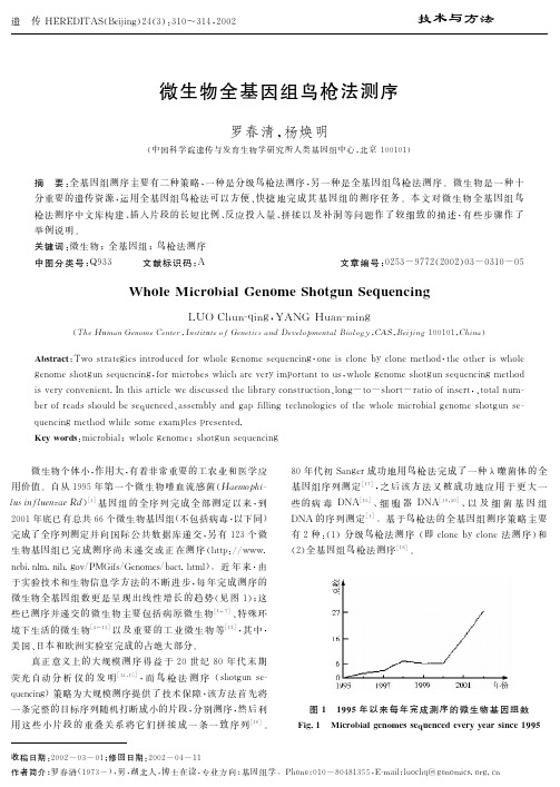
3: ; ; < >?@A>BC+,D!"#%&’E !: = ’ > :! & ’ ( ) # * ’ + $ % # . % 5 5 % 2 % ( % 9% ? % ) % + ) 5 ’ ( %: ; ; < 77 1 1 3
-!.! 82349:;<=>?@A " B?CDEFGH9: " IB?C82 3 4 F G H 9 : $ J + , C B ? K DL<M&’NO " PQ8234FGHRSTU % V W X Y Z [ 2 3 4 M 9 : \ ]$^ _ ‘ J + , 8 2 3 4 F GH9:!_abc % defgMhijk % lmn e o % pqSrstuvwxyz{|M}~" =xy k $ /01 ! J+, &8234 &FGH9: 23456 ! &!!! # $ % %!!! 789:; ! ! # 7<=6 ! " ’ ( %)$ * * ’ ’ " " ’ " %)" % ! ")" (
) !!* % ¢9:¬²³ M J + , ; < ¦ § ¨ Ñ J + , ( ÒÓÔ ) ) Q!! ’ ! % " Õª+ÖMJ + , ( S r L < M J + , u( [ !" ( ) !
Q " è + S : 1 B AZ , XQFGHYZyB? " - M 8 5

Microeconomics(8th edition)[Pindyck Rubinfeld]目录

ixCONTENTS• PART ONEIntroduction: Markets and Prices 11 Preliminaries 31.1 The Themes of Microeconomics 4Trade-Offs 4Prices and Markets 5Theories and Models 5Positive versus Normative Analysis 61.2 What Is a Market? 7Competitive versus Noncompetitive Markets 8Market Price 8Market Definition—The Extent of a Market 91.3 Real versus Nominal Prices 12 1.4 Why Study Microeconomics? 16Corporate Decision Making: The Toyota Prius 16Public Policy Design: Fuel Efficiency Standards for the Twenty-First Century 17Summary 18Questions for Review 19Exerc i ses 192 The Basics of Supply andDemand 212.1 Supply and Demand 22The Supply Curve 22The Demand Curve 232.2 The Market Mechanism 25 2.3 Changes in Market Equilibrium 26 2.4 Elasticities of Supply and Demand 33Point versus Arc Elasticities 362.5 Short-Run versus Long-Run Elasticities 39Demand 40Supply 45*2.6 Understanding and Predicting the Effects ofChanging Market Conditions 482.7 Effects of Government Intervention—PriceControls 58Summary 60Questions for Review 61Exerc i ses 62• PART TWOProducers, Consumers, and Competitive Markets 653 Consumer Behavior 67Consumer Behavior 67 3.1 Consumer Preferences 69Market Baskets 69Some Basic Assumptions about Preferences 70Indifference Curves 71Indifference Maps 72The Shape of Indifference Curves 73The Marginal Rate of Substitution 74Perfect Substitutes and Perfect Complements 753.2 Budget Constraints 82The Budget Line 82The Effects of Changes in Income and Prices 843.3 Consumer Choice 86Corner Solutions 893.4 Revealed Preference 92 3.5 Marginal Utility and Consumer Choice 95Rationing 98*3.6 Cost-of-Living Indexes 100Ideal Cost-of-Living Index 101Laspeyres Index 102Paasche Index 103Price Indexes in the United Statics: Chain Weighting 104Summary 105Questions for Review 106Exerc i ses 107Preface xviix • CONTENTS5 Uncertainty and ConsumerBehavior 1595.1 Describing Risk 160Probability 160Expected Value 161Variability 161Decision Making 1635.2 Preferences Toward Risk 165Different Preferences Toward Risk 1665.3 Reducing Risk 170Diversification 170Insurance 171The Value of Information 174*5.4 The Demand for Risky Assets 176Assets 176Risky and Riskless Assets 177Asset Returns 177The Trade-Off Between Risk and Return 179The Investor’s Choice Problem 1805.5 Bubbles 185Informational Cascades 1875.6 Behavioral Economics 189Reference Points and Consumer Preferences 190Fairness 192Rules of Thumb and Biases in Decision Making 194Summing Up 196Summary 197Questions for Review 197Exerc i ses 1986 Production 201The Production Decisions of a Firm 201 6.1 Firms and Their Production Decisions 202Why Do Firms Exist? 203The Technology of Production 204The Production Function 204The Short Run versus the Long Run 2056.2 Production with One Variable Input (Labor) 206Average and Marginal Products 206The Slopes of the Product Curve 207The Average Product of Labor Curve 209The Marginal Product of Labor Curve 209The Law of Diminishing Marginal Returns 209Labor Productivity 2146.3 Production with Two Variable Inputs 216Isoquants 2164 Individual and MarketDemand 1114.1 Individual Demand 112Price Changes 112The Individual Demand Curve 112Income Changes 114Normal versus Inferior Goods 115Engel Curves 116Substitutes and Complements 1184.2 Income and Substitution Effects 119Substitution Effect 120Income Effect 121A Special Case: The Giffen Good 1224.3 Market Demand 124From Individual to Market Demand 124Elasticity of Demand 126Speculative Demand 1294.4 Consumer Surplus 132Consumer Surplus and Demand 1324.5 Network Externalities 135Positive Network Externalities 135Negative Network Externalities 137*4.6 Empirical Estimation ofDemand 139The Statistical Approach to Demand Estimation 139The Form of the Demand Relationship 140Interview and Experimental Approaches to Demand Determination 143Summary 143Questions for Review 144Exerc i ses 145APPENDIX TO CHAPTER 4:Demand Theory—A Mathematical Treatment 149Utility Maximization 149The Method of Lagrange Multipliers 150The Equal Marginal Principle 151Marginal Rate of Substitution 151Marginal Utility of Income 152An Example 153Duality in Consumer Theory 154Income and Substitution Effects 155Exerc i ses 157CONTENTS • xiAPPENDIX TO CHAPTER 7:Production and Cost Theory—A Mathematical Treatment 273Cost Minimization 273Marginal Rate of Technical Substitution 274Duality in Production and Cost Theory 275The Cobb-Douglas Cost and Production Functions 276Exerc i ses 2788 Profit Maximization andCompetitive Supply 2798.1 Perfectly Competitive Markets 279When Is a Market Highly Competitive? 2818.2 Profit Maximization 282Do Firms Maximize Profit? 282Alternative Forms of Organization 2838.3 Marginal Revenue, Marginal Cost, and ProfitMaximization 284Demand and Marginal Revenue for a Competitive Firm 285Profit Maximization by a Competitive Firm 2878.4 Choosing Output in the Short Run 287Short-Run Profit Maximization by a Competitive Firm 287When Should the Firm Shut Down? 2898.5 The Competitive Firm’s Short-Run SupplyCurve 292The Firm’s Response to an Input Price Change 2938.6 The Short-Run Market Supply Curve 295Elasticity of Market Supply 296Producer Surplus in the Short Run 2988.7 Choosing Output in the Long Run 300Long-Run Profit Maximization 300Long-Run Competitive Equilibrium 301Economic Rent 304Producer Surplus in the Long Run 3058.8 The Industry’s Long-Run SupplyCurve 306Constant-Cost Industry 307Increasing-Cost Industry 308Decreasing-Cost Industry 309The Effects of a Tax 310Long-Run Elasticity of Supply 311Summary 314Questions for Review 314Exerc i ses 315Input Flexibility 217Diminishing Marginal Returns 217Substitution Among Inputs 218Production Functions—Two Special Cases 2196.4 Returns to Scale 223Describing Returns to Scale 224Summary 226Questions for Review 226Exerc i ses 2277 The Cost of Production 2297.1 Measuring Cost: Which Costs Matter? 229Economic Cost versus Accounting Cost 230Opportunity Cost 230Sunk Costs 231Fixed Costs and Variable Costs 233Fixed versus Sunk Costs 234Marginal and Average Cost 2367.2 Cost in the Short Run 237The Determinants of Short-Run Cost 237The Shapes of the Cost Curves 2387.3 Cost in the Long Run 243The User Cost of Capital 243The Cost-Minimizing Input Choice 244The Isocost Line 245Choosing Inputs 245Cost Minimization with Varying Output Levels 249The Expansion Path and Long-Run Costs 2507.4 Long-Run versus Short-Run Cost Curves 253The Inflexibility of Short-Run Production 253Long-Run Average Cost 254Economies and Diseconomies of Scale 255The Relationship between Short-Run and Long-Run Cost 2577.5 Production with Two Outputs—Economies ofScope 258Product Transformation Curves 258Economies and Diseconomies of Scope 259The Degree of Economies of Scope 259*7.6 Dynamic Changes in Costs—The LearningCurve 261Graphing the Learning Curve 261Learning versus Economies of Scale 262*7.7 Estimating and Predicting Cost 265Cost Functions and the Measurement of Scale Economies 267Summary 269Questions for Review 270Exerc i ses 271xii • CONTENTS10.5 Monopsony 382Monopsony and Monopoly Compared 38510.6 Monopsony Power 385Sources of Monopsony Power 386The Social Costs of Monopsony Power 387Bilateral Monopoly 38810.7 Limiting Market Power: The AntitrustL aws 389Restricting What Firms Can Do 390Enforcement of the Antitrust Laws 391Antitrust in Europe 392Summary 395Questions for Review 395Exerc i ses 39611 Pricing with Market Power 39911.1 Capturing Consumer Surplus 400 11.2 Price Discrimination 401First-Degree Price Discrimination 401Second-Degree Price Discrimination 404Third-Degree Price Discrimination 40411.3 Intertemporal Price Discrimination andPeak-Load Pricing 410Intertemporal Price Discrimination 411Peak-Load Pricing 41211.4 The Two-Part Tariff 414 *11.5 Bundling 419Relative Valuations 420Mixed Bundling 423Bundling in Practice 426Tying 428*11.6 Advertising 429A Rule of Thumb for Advertising 431Summary 434Questions for Review 434Exerc i ses 435APPENDIX TO CHAPTER 11:The Vertically Integrated Firm 439Why Vertically Integrate? 439Market Power and Double M arginalization 439Transfer Pricing in the Integrated Firm 443Transfer Pricing When There Is No Outside Market 443Transfer Pricing with a Competitive Outside Market 4469 The Analysis of CompetitiveMarkets 3179.1 Evaluating the Gains and Losses fromGovernment Policies—Consumer and Producer Surplus 317Review of Consumer and Producer Surplus 318Application of Consumer and Producer Surplus 3199.2 The Efficiency of a Competitive Market 323 9.3 Minimum Prices 328 9.4 Price Supports and Production Quotas 332Price Supports 332Production Quotas 3339.5 Import Quotas and Tariffs 340 9.6 The Impact of a Tax or Subsidy 345The Effects of a Subsidy 348Summary 351Questions for Review 352Exerc i ses 352• PART THREEMarket Structure and CompetitiveStrategy 35510 Market Power: Monopolyand Monopsony 35710.1 Monopoly 358Average Revenue and Marginal Revenue 358The Monopolist’s Output Decision 359An Example 361A Rule of Thumb for Pricing 363Shifts in Demand 365The Effect of a Tax 366*The Multiplant Firm 36710.2 Monopoly Power 368Production, Price, and Monopoly Power 371Measuring Monopoly Power 371The Rule of Thumb for Pricing 37210.3 Sources of Monopoly Power 375The Elasticity of Market Demand 376The Number of Firms 376The Interaction Among Firms 37710.4 The Social Costs of Monopoly Power 377Rent Seeking 378Price Regulation 379Natural Monopoly 380Regulation in Practice 381CONTENTS • xiii13.6 Threats, Commitments, and Credibility 505Empty Threats 506Commitment and Credibility 506Bargaining Strategy 50813.7 Entry Deterrence 510Strategic Trade Policy and International Competition 512*13.8 Auctions 516Auction Formats 517Valuation and Information 517Private-Value Auctions 518Common-Value Auctions 519Maximizing Auction Revenue 520Bidding and Collusion 521Summary 524Questions for Review 525Exerc i ses 52514 Markets for Factor Inputs 52914.1 Competitive Factor Markets 529Demand for a Factor Input When Only One Input Is Variable 530Demand for a Factor Input When Several Inputs Are Variable 533The Market Demand Curve 534The Supply of Inputs to a Firm 537The Market Supply of Inputs 53914.2 Equilibrium in a Competitive FactorMarket 542Economic Rent 54214.3 Factor Markets with Monopsony Power 546Monopsony Power: Marginal and Average Expenditure 546Purchasing Decisions with Monopsony Power 547Bargaining Power 54814.4 Factor Markets with Monopoly Power 550Monopoly Power over the Wage Rate 551Unionized and Nonunionized Workers 552Summary 555Questions for Review 556Exerc i ses 55615 Investment, Time, and CapitalMarkets 55915.1 Stocks versus Flows 560 15.2 Present Discounted Value 561Valuing Payment Streams 562Transfer Pricing with a Noncompetitive Outside M arket 448Taxes and Transfer Pricing 448A Numerical Example 449Exerc i ses 45012 Monopolistic Competition andOligopoly 45112.1 Monopolistic Competition 452The Makings of Monopolistic Competition 452Equilibrium in the Short Run and the Long Run 453Monopolistic Competition and Economic Efficiency 45412.2 Oligopoly 456Equilibrium in an Oligopolistic Market 457The Cournot Model 458The Linear Demand Curve—An Example 461First Mover Advantage—The Stackelberg M odel 46312.3 Price Competition 464Price Competition with Homogeneous Products— The Bertrand Model 464Price Competition with Differentiated Products 46512.4 Competition versus Collusion: The Prisoners’Dilemma 46912.5 Implications of the Prisoners’ Dilemma forOligopolistic Pricing 472Price Rigidity 473Price Signaling and Price Leadership 474The Dominant Firm Model 47612.6 Cartels 477Analysis of Cartel Pricing 478Summary 482Questions for Review 482Exerc i ses 48313 Game Theory and CompetitiveStrategy 48713.1 Gaming and Strategic Decisions 487Noncooperative versus Cooperative Games 48813.2 Dominant Strategies 490 13.3 The Nash Equilibrium Revisited 492Maximin Strategies 494*Mixed Strategies 49613.4 Repeated Games 498 13.5 Sequential Games 502The Extensive Form of a Game 503The Advantage of Moving First 504xiv • CONTENTS16.4 Efficiency in Production 613Input Efficiency 613The Production Possibilities Frontier 614Output Efficiency 615Efficiency in Output Markets 61716.5 The Gains from Free Trade 618Comparative Advantage 618An Expanded Production Possibilities Frontier 61916.6 An Overview—The Efficiency of CompetitiveMarkets 62316.7 Why Markets Fail 625Market Power 625Incomplete Information 625Externalities 626Public Goods 626Summary 627Questions for Review 628Exerc i ses 62817 Markets with AsymmetricInformation 63117.1 Quality Uncertainty and the Market forL emons 632The Market for Used Cars 632Implications of Asymmetric Information 634The Importance of Reputation and Standardization 63617.2 Market Signaling 638A Simple Model of Job Market Signaling 639Guarantees and Warranties 64217.3 Moral Hazard 643 17.4 The Principal–Agent Problem 645The Principal–Agent Problem in Private Enterprises 646The Principal–Agent Problem in Public Enterprises 648Incentives in the Principal–Agent Framework 650*17.5 Managerial Incentives in an IntegratedFirm 651Asymmetric Information and Incentive Design in the Integrated Firm 652Applications 65417.6 Asymmetric Information in Labor Markets:Efficiency Wage Theory 654Summary 656Questions for Review 657Exerc i ses 65715.3 The Value of a Bond 564Perpetuities 565The Effective Yield on a Bond 56615.4 The Net Present Value Criterion for CapitalInvestment Decisions 569The Electric Motor Factory 570Real versus Nominal Discount Rates 571Negative Future Cash Flows 57215.5 Adjustments for Risk 573Diversifiable versus Nondiversifiable Risk 574The Capital Asset Pricing Model 57515.6 Investment Decisions by Consumers 578 15.7 Investments in Human Capital 580 *15.8 Intertemporal Production Decisions—Depletable Resources 584The Production Decision of an Individual Resource Producer 584The Behavior of Market Price 585User Cost 585Resource Production by a Monopolist 58615.9 How Are Interest Rates Determined? 588A Variety of Interest Rates 589Summary 590Questions for Review 591Exerc i ses 591• PART FOURInformation, Market Failure, andthe Role of Government 59316 General Equilibrium and EconomicEfficiency 59516.1 General Equilibrium Analysis 595Two Interdependent Markets—Moving to General Equilibrium 596Reaching General Equilibrium 597Economic Efficiency 60116.2 Efficiency in Exchange 602The Advantages of Trade 602The Edgeworth Box Diagram 603Efficient Allocations 604The Contract Curve 606Consumer Equilibrium in a Competitive Market 607The Economic Efficiency of Competitive M arkets 60916.3 Equity and Efficiency 610The Utility Possibilities Frontier 610Equity and Perfect Competition 612CONTENTS • xv18.7 Private Preferences for Public Goods 694Summary 696Questions for Review 696Exerc i ses 697APPENDIX:The Basics of Regression 700An Example 700Estimation 701Statistical Tests 702Goodness of Fit 704Economic Forecasting 704Summary 707Glossary 708Answers to Selected Exercises 718Photo Credits 731Index 73218 Externalities and PublicGoods 66118.1 Externalities 661Negative Externalities and Inefficiency 662Positive Externalities and Inefficiency 66418.2 Ways of Correcting Market Failure 667An Emissions Standard 668An Emissions Fee 668Standards versus Fees 669Tradeable Emissions Permits 671Recycling 67518.3 Stock Externalities 678Stock Buildup and Its Impact 67918.4 Externalities and Property Rights 684Property Rights 684Bargaining and Economic Efficiency 685Costly Bargaining—The Role of Strategic Behavior 686A Legal Solution—Suing for Damages 68618.5 Common Property Resources 687 18.6 Public Goods 690Efficiency and Public Goods 691Public Goods and Market Failure 692。

高通量微生物多样性分析方案

微基生物，将继续围绕微生物多样性分析核心业务，紧跟国际分子生物学技术、生物信息学、统计分析技术収展，以优良的服务质量，协助研究者解码微生物世界的奥秘！
微基生物科技（上海）有限公司
3 / 36
微基生物——解码微生物的奥秘
二、微基生物代表客户及项目列表
合作单位
涉及领域
复旦大学
同济大学清华大学深圳研究生院
国家海洋局第一海洋研究所
东海水产研究所光明乳业股份有限公司
乳业研究院陕西省微生物研究所中科院上海高等研究院
土壤微生物
淤泥微生物鱼肠道微生物
乳品微生物
河流微生物淤泥微生物
中国极地研究中心
南海水产研究所
昆虫肠道微生物淤泥微生物
分析平台 PCR-DGGE 高通量测序平台高通量测序平台高通量测序平台高通量测序平台高通量测序平台 PCR-DGGE 高通量测序平台高通量测序平台高通量测序平台高通量测序平台高通量测序平台高通量测序平台 PCR-DGGE
微基生物是国内唯一一家同时具有 PCR-DGGE 平台、454 及公司。公司拥有经验丰富的技术团队，涉及分子生物学、生态学、生物信息学、统计学方面，团队核心成员具有 10 余年一线科研工作经验。
微基生物已完成 300 余项微生物多样性分析项目，分析样本 6000 余例。研究对象涉及土壤、粪便、水体、肠道、収酵物、人体微生物等各类样本，代表客户有中科院、清华大学、复旦大学、同济大学、新华医院、中山医院、海洋研究所、中国极地研究中心等众多科研客户及乳制品、化妆品行业内的企业客户。
1、细菌多样性分析 ............................................................................................... 9 2、真核生物多样性分析 ...................................................................................... 10 3、真菌多样性分析 ............................................................................................. 11 4、古菌多样性分析 ............................................................................................. 13 5、指定功能微生物多样性分析： ....................................................................... 15 五、建库流程.........................................................................................................................17 1. 微基优势： ...............................................................................................................17 2. 建库实验步骤：........................................................................................................17 2.1 基因组 DNA 抽提 ...................................................................................................17 2.2 PCR 引物的设计 ...................................................................................................18 2.3 PCR 扩增 ...............................................................................................................18 2.4 PCR 产物的凝胶回收及检测 ...............................................................................19 2.5 已送样品的 Qubit 2.0 DNA 定量 .........................................................................19 六、生物信息学分析流程.....................................................................................................20 1、测序数据统计分析...............................................................................................20 2、OTU-based 分析 .......................................................................................................21 3、多样性分析（Alpha-diversity）............................................................................22 4、稀释性曲线（Rarefaction curve） ..........................................................................23 5、分类学分析（Taxonomy）....................................................................................25 6、各样本间不同分类水平的比较.............................................................................27 7、全样本相似度分析.................................................................................................28 8、样品 OTU 分布比较-VENN 图 ..............................................................................29 9、 Heatmap ..................................................................................................................30 10、 PCA 分析(Principal Component Analysis)...........................................................31 11、 RDA 分析(Redundancy Analysis) ........................................................................32 七、高级数据分析及绘图服务.............................................................................................34 1、微生物种类分级进化树分析 ................................................................................... 34 2、网络图分析方案 ....................................................................................................... 35 3、进化树分析 ............................................................................................................... 35 联系方式：..................................................................................................................................... 36

宏蛋白组学Metaproteomics

一些新的能够快速检测和鉴定新的微生物的方法
• 宏基因组学（metagenomics）：又叫微生物环境基因组学，元基因组学。自然界约99%的微生物不能通过传统的分离筛选途径进行培养（即未培养微生物）,为获得新的基因资源,更全面地认识微生物多样性和微生物在自然环境和生物圈中的重要作用，近年来随着分子生物学的快速发展及其在微生物研究中的广泛运用,以环境中未培养微生物为研究对象的新兴学科 • 可利用环境微生物基因组技术进行土壤污染修复、畜禽养殖除臭、鉴定新物种以及确定特定生态环境体系中未培养微生物种群与群落的结构组成及物种的进化模式
宏基因组学研究策略
• 从环境样品中提取并纯化微生物群体基因组： • 构建环境基因组： • 环境基因组的筛选分析：
宏蛋白组学(Metaproteomics):是由Paul和Philip二人在2004年首先提出，是应用蛋白质组学技术对微生物群落进行研究的一项新技术，其定义为在特定的时间对微生物群落的所有蛋白质组成进行大规模鉴定 . 近年来，人们已经意识到微生物在自然界中的重要作用，它们是生态系统中各种元素循环不可或缺的一环，而且它们大多具有许多独特的生物功能，如有些微生物对各种复杂有机化合物有降解作用、有些微生物可以在一些极端环境下生存等等，而使微生物具有这些独特功能的是一些特殊的酶．众所周知，大多数酶的化学本质是蛋白质，因此对不同自然生态环境中所有的蛋白质的研究就显得特别重要，宏蛋白质组学就是在这种背景下诞生的．
Байду номын сангаас在全球性的改变方面发挥关键的作用。
2，微生物对三个主要的全球性问题，包括能源安
全，环境方面面临的挑战和传染疾病的解决方案。
微生物体已经被广泛的开发用于医药，农业，食品和工业上

pmirGLO vector

Promega Corporation2800 Woods Hollow Road Madison, WI 53711-5399USA Telephone 608-274-4330Toll Free 800-356-9526Fax 608-277-2516InternetPRODUCT USE LIMITATIONS, WARRANTY,DISCLAIMER Promega manufactures products for a number of intended uses. Please refer to the product label for the intended use statements for specific products.Promega products contain chemicals which may be harmful if misused. Due care should be exercised with all Promega products to prevent direct human contact.Each Promega product is shipped with documentation stating specifications and other technical information.Promega products are warranted to meet or exceed the stated specifications. Promega's sole obligation and the customer's sole remedy is limited to replace-ment of products free of charge in the event products fail to perform as warranted. Promega makes no other warranty of any kind whatsoever, and SPECIFICALLY DISCLAIMS AND EXCLUDES ALL OTHER WAR-RANTIES OF ANY KIND OR NATURE WHATSOEVER,DIRECTLY OR INDIRECTLY, EXPRESS OR IMPLIED,INCLUDING, WITHOUT LIMITATION, AS TO THESUITABILITY, PRODUCTIVITY, DURABILITY, FITNESS FOR A PARTICULAR PURPOSE OR USE, MER-CHANTABILITY, CONDITION, OR ANY OTHER MAT-TER WITH RESPECT TO PROMEGA PRODUCTS. In no event shall Promega be liable for claims for any other damages, whether direct, incidental, foresee-able, consequential, or special (including but not lim-ited to loss of use, revenue or profit), whether based upon warranty, contract, tort (including negligence) or strict liability arising in connection with the sale or the failure of Promega products to perform in accordance with the stated specifications.Part# 9PIE133Revised 10/09Part# 9PIE133Printed in USA Revised 10/09pmirGLO Dual-Luciferase miRNA Target Expression Vector:Cat.#Size E133020µgC a t .# E 1330 c o n t a i n s :P a r t N o .N a m e E133A pmirGLO Vector 20µg C838A Oligo Annealing Buffer1mlDescription: The pmirGLO Dual-Luciferase miRNA Target Expression Vector (a–e)is designed to quantitatively evaluate microRNA (miRNA) activity by the insertion of miRNA target sites 3´ of the firefly luciferase gene (luc2). These target sites can be introduced by cloning putative miRNA binding sites alone, or the 3´ untranslated region (UTR) of a gene of interest, to study the influence of these sites on transcript stability and activity. Firefly luciferase is the primary reporter gene;reduced firefly luciferase expression indicates the binding of endogenous or introduced miRNAs to the cloned miRNA target sequence. This vector is based on Promega dual-luciferase technology, with firefly luciferase (luc2) used as the primary reporter to monitor mRNA regulation and Renilla luciferase (hRluc-neo ) acting as a control reporter for normalization and selection. This vector contains the following features:•Human phosphoglycerate kinase (PGK) promoter provides low translational expression, which is advantageous when reduction of signal is the desired response. The PGK promoter is a nonviral universal promoter, which functions across cell lines (yeast, rat, mouse and human).•Firefly luciferase reporter gene (luc2) inversely reports miRNA activity in mammalian cells.•Multiple cloning site (MCS) is located 3´ of the firefly luciferase reporter gene (luc2).•Humanized Renilla luciferase-neomycin resistance cassette (hRluc -neo) is used as a control reporter for normalization of gene expression and stable cell line selection.•Amp r gene allows bacterial selection for vector amplification.•SV40 late poly(A) signal sequence is positioned downstream of luc2to provide efficient transcription termination and mRNA polyadenylation.•Synthetic poly(A) signal/transcription stop site.Concentration: 1µg/µl in 10mM Tris-HCl, 1mM EDTA; final pH 7.4.GenBank ®Accession Number:FJ376737.Storage Conditions:See the storage temperature and expiration date on the Product Information Label.Functional AssaysIdentity Assay: The vector has been sequenced completely and has 100% identity with the published sequence availableat: ww w w .p r o m e g a .c o m /v e c t o r s /Restriction Digestion:The functional purity of this vector DNA is verified by complete digestion with restriction enzymes at the optimal temperature for 1 hour. Samples are examined by agarose gel electrophoresis, comparing cut and uncut vector DNA with marker DNA.Contaminant AssaysContaminating Nucleic Acids: RNA, single-stranded DNA and chromosomal DNA are not evident in specified quantities of this vector as determined by agarose gel electrophoresis.Nuclease Assay: Following incubation of 1µg of this vector in Restriction Enzyme Buffer at 37°C for 16–24 hours, no evidence of nuclease activity is detected by agarose gel electrophoresis.Physical Purity:A 260/A 280≥1.80, A 260/A 250≥1.05.© 2008, 2009 Promega Corporation. All Rights Reserved.Dual-Glo is a registered trademark of Promega Corporation. GeneClip and PureYield are trademarks of Promega Corporation.GenBank is a registered trademark of US Department of Health and Human Services.Products may be covered by pending or issued patents or may have certain limitations. Please visit our Web site for more information.All specifications are subject to change without prior notice.Product claims are subject to change. Please contact Promega Technical Services or access the Promega online catalog for the most up-to-date information on Promega products.AF9PI E133 1009E133(a)READ THIS FIRST BEFORE OPENING PRODUCTThe sale of this product and its use by the purchaser are subject to the terms of a limited use label license, the full text of which is shippedwith this product and also available at: ww w w .p r o m e g a .c o m \L U L L . That text must be read by the purchaser prior to opening this product to determine whether the purchaser agrees that all use of the product shall be in accordance with the license terms. If the purchaser is not willing to accept the terms of the limited use label license, Promega is willing to accept the return of the unopened product and provide the purchaser with a full refund. However, if the product is opened for any reason, then the purchaser agrees to be bound by the terms of the limited use label license.(b)U.S. Pat. No. 5,670,356.(c)Australian Pat. No. 2001 285278 and other patents pending.(d)The method of recombinant expression of Coleoptera luciferase is covered by U.S. Pat. Nos. 5,583,024, 5,674,713 and 5,700,673. A license (from Promega for research reagent products and from The Regents of the University of California for all other fields) is needed for any commercial sale of nucleic acid contained within or derived from this product.(e)Licensed from University of Georgia Research Foundation, Inc., under U.S. Pat. Nos. 5,292,658, 5,418,155, Canadian Pat. No.2,105,984 and related patents.S i g n e d b y :J. Stevens, Quality AssurancePromega Corporation2800 Woods Hollow Road·Madison, WI 53711-5399 U.S.A. Toll Free in the USA 800-356-9526 Telephone 608-274-4330 Features List and Map for the pmirGLO VectorSV40 late poly(A) signal106–327SV40 early enhancer/promotor426–844hRluc -neo fusion protein coding region 889–2664Synthetic polyadenylation signal 2728–2776β-lactamase (Amp r ) coding region3037–3897Col E1-derived plasmid origin of replication 4052–4088Human phosphoglycerate kinase promoter 5094–5609luc2reporter gene5645–7297Multiple cloning site (MCS, Figure 1)7306–7350I.Sample ProtocolA.Vector Cloning1.Design oligonucleotides: Order oligonucleotide pairs that contain the desired miRNAtarget region and, when annealed and ligated into the pmirGLO Vector, result in the miRNA target region in the correct 5´ to 3´ orientation. Insure that the overhangs created by oligonucleotide annealing are complementary to those generated by restric-tion enzyme digestion of the pmirGLO Vector in Step 2. Add an internal restriction site to your oligonucleotides for clone confirmation (e.g., NotI in Figure 3 creates a ~125bp insert when digested with NotI because of a NotI site at position 93 in the vector).2.Digest vector: Linearize the pmirGLO Vector with the appropriate restriction enzymes togenerate overhangs that are complementary to the annealed oligonucleotide overhangs.3.Anneal oligonucleotides: Dilute both oligonucleotides (supplied by user) to 1µg/µl.Combine 2µl of each oligonucleotide with 46µl of Oligo Annealing Buffer. Heat at 90°C for 3 minutes, then transfer to a 37°C water bath for 15 minutes. Use the annealed oligonucleotides immediately, or store at –20°C.B.Ligation and Transformation1.Dilute annealed oligonucleotides 1:10 in nuclease-free water to a final concentrationof 4ng/µl per oligonucleotide. Ligate 4ng of annealed oligonucleotides and 50ng of linearized vector using a standard ligation protocol. Transform ligated pmirGLO Vector using high-efficiency JM109 competent cells (e.g., Cat.# L2001).2.Select clones on ampicillin-containing plates, then select clones containing theoligonucleotides by digesting miniprep-purified DNA (e.g., purified using thePureYield™ Plasmid Miniprep System, Cat.# A1221) using the unique restriction site in the oligonucleotide pair. The purified plasmid DNA can be transfected directly or expanded to generate more DNA.Additional information about annealing, ligation, transformation and oligonucleotide design can be found in the GeneClip ™ U1 Hairpin Cloning Systems Technical Manual ,C.An Example of Detecting mi-R21 Activity Using the pmirGLO Vector:miR-21 ConstructAn overview describing the use of the pmirGLO Vector to interrogate endogenous mi-R21microRNA is shown in Figure 2.The presence of broadly endogenous microRNA mi-R21 was monitored in HeLa cells.Constructs contained either an exact match to the 21bp mi-R21 target sequence or a mismatched version of that target site (1) as well as PmeI, XbaI and NotI restriction sites (Figure 3; mismatched sequence is in italics). Twenty-four hours after transfection with the mi-R21 pmirGLO Vector constructs, cells were analyzed for luciferase activity using the Dual-Glo ®Luciferase Assay System (Cat.# E2920) and a MicroLumatPlus LB96V lumino-meter (Berthold). Normalized firefly luciferase activity (firefly luciferase activity/Renilla luciferase activity) for each construct was compared to that of the pmirGLO Vector no-insert control. For each transfection, luciferase activity was averaged from six replicates.II.Reference1.Zeng, Y. and Cullen, B.R. (2003) Sequence requirements for micro RNA processing-neo SV40 late PGK ...GCAAG ATCGC CGTGT AATTC TAGTT GTTTA AACGA GCTCG CTAGCCTCGA GTCTA GAGTC GACCT GCAGG...PmeI DraI 5´EcoICRI Sac INheIXhoI SalI AccIXbaI3´F i g u r e 1. p m i rG L O V e c t o r m u l t i p l e c l o n i ng s i te .gene firefly luciferase translation In absence of mi-R21activity.proteinmRNA destablized;F i g u r e 2. M e c h a n i s m o f a c t i o n o f t h e p m i r G L O V e c t o r .5´ CTAGA TAGCTTATC TT CTGATGTTGA ACTA GCGGCCGC TA GTTT 3´XbaImi-R21 mismatch sense, PmeI and XbaImi-R21 antisense, PmeI and XbaImi-R21 sense, PmeI and XbaImi-R21 mismatch antisense, PmeI and XbaI5´ AAAC TA GCGGCCGC TAGT TCAACATCAG TCT GATAAGCTA T 3´5´ CTAGA TAGCTTATC AGA CTGATGTTGA ACTA GCGGCCGC TA GTTT 3´5´ AAAC TA GCGGCCGC TAGT TCAACATCAG AA GATAAGCTA T 3´PmeI NotI internal sitemi-R21 target sequence XbaIPmeINotI internal site mi-R21 target sequence F i g u r e 3. S a m p l e o l i g o n u c l e o t i d e s f o rm i -R 21.mismatchP e r c e n t f i r e f l y :R e n i l l a l u c i f e r a s e a c t i v i t y c o m p a r e d t o n o -i n s e r t c o n t r o lF i g u r e 4. N o r m a l i z e d l u c i f e r a s e a c t i v i t y u s i n g t h e p m i rG L O V e c t o r w i t h a n m i -R 21 t a r g e t s e q u e n c e .。

单细胞转录组应用发展历史

单细胞转录组应用发展历史
单细胞转录组应用的发展历史可以追溯到2009年，当时北京大学的汤富酬老师等人通过对少数小鼠原始生殖细胞进行高通量测序，实现了在单个细胞中对mRNA全基因组的检测。

此后，单细胞转录组学技术不断发展创新，出现了标签测序方法（如strt-seq和cel-seq，mars-seq）和全长测序（如Smart-seq/Smart-seq2）等。

直到2015年，10X genomics公司开发了构建基因组大片段Linked Reads文库的技术，用于辅助基因组组装拼接。

2016年，该公司将其技术应用范围拓展到了单细胞测序领域，推出了单细胞转录组测序产品。

该产品通过测定mRNA 3’端或5’端实现定量，具有更高的性价比。

2017年，10X genomics公司推出了单细胞免疫组库（V(D)J-seq）产品，用于检测免疫细胞（如B淋巴细胞、T淋巴细胞、自然杀伤细胞和树突状细胞等）的数量和功能变化。

单细胞转录组应用的发展得益于测序技术的不断进步和创新，为生物学研究提供了更加深入和细致的分析方法。

一种新的多肽——核糖体蛋白S10 14和编码这种多肽的多核苷酸[发明专利]

专利名称：一种新的多肽——核糖体蛋白S10 14和编码这种多肽的多核苷酸
专利类型：发明专利
发明人：毛裕民,谢毅
申请号：CN99125390.6
申请日：19991227
公开号：CN1301725A
公开日：
20010704
专利内容由知识产权出版社提供
摘要：本发明公开了一种新的多肽——核糖体蛋白S1014,编码此多肽的多核苷酸和经DNA重组技术产生这种多肽的方法。

本发明还公开了此多肽用于治疗多种疾病的方法,如恶性肿瘤,血液病,HIV感染和免疫性疾病和各类炎症等。

本发明还公开了抗此多肽的拮抗剂及其治疗作用。

本发明还公开了编码这种新的核糖体蛋白S1014的多核苷酸的用途。

申请人：上海博德基因开发有限公司
地址：200092 上海市中山北二路1111号3号楼12层
国籍：CN
更多信息请下载全文后查看。

Microeconomic Probset3_solution

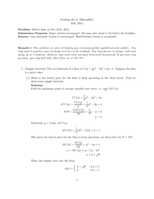
Problem Set 2:MEcon6021Fall,2014Deadline:Before 6pm on Nov 21th,2014.Submission Channels:Paper version encouraged.You may also email to TA before the deadline.Format:type-and-print version is encouraged.Handwriting version is acceptable.Remark 1This problem set aims at helping you reviewing partial equilibrium and welfare.You may want to practice more by doing exercises in the textbook.You may discuss in groups,with each group up to 5students.However,you must write out your homework by yourself.If you have any question,you may ﬁnd help either from me or the TA.1.(Supply function)The cost function of a ﬁrm is C (y )=13y 3−2y 2+4y +1.Suppose the ﬁrmis a price taker.(a)What is the lowest price for the ﬁrm to keep operating in the short term?Find itsshort-term supply function.Solution:Find the minimum point of average variable cost curve,i.e.min yAV C (y )V C (y )=13y 3−2y 2+4y AV C (y )=V C (y )y =13y 2−2y +4F OC :∂AV C (y )∂y =23y −2=0y =3Substitute y =3into AV C (y ),AV C (3)=13(3)2−2(3)+4=1This gives the lowest price for the ﬁrm to keep operation,we then solve for P =MCMC (y )=∂C (y )∂y=y 2−4y +4p =MC (y )⇒p =(y −2)2y =2+√pThus,the supply curve has the formy (p )= 2+√p if p ≥10if p <11(b)What is the lowest price for the ﬁrm to keep operating in the long term?Find itslong-term supply function.Solution:Find the minimum point of average cost curve,i.e.min yAC (y )AC (y )=C (y )y =13y 2−2y +4+1yF OC :∂AC (y )∂y =23y −2−1y2=0y =3.1511Substitute y =3.1511into AC (y ),AC (3.1511)=13(3.1511)2−2(3.1511)+4+13.1511=1.325This gives the lowest price for the ﬁrm to keep operation.Thus,the supply curve has the form y (p )= 2+√p if p ≥1.3250if p <1.3252.(Short-term competitive equilibrium)The market demand function is:X (p )=21−5p .There are 5identical ﬁrms with ﬁrm cost function C (y )=y 2+1.2.(a)Solve for the short-term competitive equilibrium price and number of ﬁrms in the market.Solution:Solve for p =MCMC (y )=∂C (y )∂y=2y p =MC (y )⇒p =2y y =p 2Since AV C (y )=y <2y =MC (y )(or min y AV C (y )=0),we have y =p/2as the supplyfunction for all p >0,we then calculate market supplyY (p )=p 2m =5p 2Market clearing conditionX (p )=Y (p )⇒21−5p =5p2p =2.8y =p 2=1.4Y =5y =7Since p >0,all ﬁrms will continue to operate.2(b)What is the proﬁt for eachﬁrm?Solution:π=py−C(y)=2.8(1.4)−(1.42+1.2)=0.763.(Long-term competitive equilibrium)In the above question,suppose there is no barrier forentry and exit.(a)What will happen when otherﬁrms see the result you get in the above question.Solution:The otherﬁrms will enter to the market becauseπ>0.(b)Solve for the long-term equilibrium price,output,and number ofﬁrms in the market.Solution:Market clearing conditionX(p)=Y(p)⇒21−5p=mp 2p=42 m+10Use the zero proﬁt condition andﬁnd the minimum point of average cost curveAC(y)=C(y)y=y+1.2yF OC:∂AC(y)∂y=1−1.2y2=0y=√1.2AC(√1.2)=√1.2+1.2√1.2=2.1909Substitute p=2.1909into the market clearing condition2.1909=42 m+10m=9.1702Since the largest integer lower than9.1702is9,thus we have m=9.In the long-term equilibriump=429+10=2.2105Y=21−5p=9.9475y=Y/m=1.1053(1)(c)Compute the consumer surplus,producer surplus,and total surplus.Solution:CS=(215−2.2105)(9.9475)(12)=9.8953P S=(2.2105)(9.9475)(12)=10.9945T S=CS+P S=20.8898(2) 34.(Welfare)In the above question,suppose government levies a quantity sales tax of t=0.3.(a)Find the new long-term equilibrium price,output,and number ofﬁrms.Solution:Suppose p is the price received by the sellers.Then the price paid by the buyers will be p+0.3.Find the market clearing conditionX(p+t)=Y(p,m)⇒21−5(p+0.3)=mp 2p=39 m+10Use the zero proﬁt condition from Q3,substitute p=2.1909into the market clearing condition2.1909=39 m+10m=7.8009Since the largest integer lower than7.8009is7,thus we have m=7.In the long-run equilibriump=397+10=2.2941Y=21−5(p+0.3)=8.0295y=Y/m=1.1471(3)(b)Compute the consumer surplus,producer surplus,and total surplus.Solution:CS=[215−(2.2941+0.3)](8.0295)(12)=6.4473P S=(2.2941)(8.0295)(12)=9.2102T ax=(0.3)(8.0295)=2.4089T S=CS+P S+T ax=18.0664(4)(c)How does government tax aﬀect social welfare(total surplus)?Show your idea with aclearly deﬁned graph.Solution:Total surplus(or social welfare)is decreased from20.8898to18.0664.Both demand and supply will shift in.The new equilibrium rests on a lower output level and an(almost) unchanged price.5.(First-Best Allocation)Consider an exchange economy with two consumers(1and2)and twogoods(A and B).The preference of both consumers are given as u1(x1A,x1B)=x1/21A x1/2 1B,u2(x2A,x2B)=x1/22A x1/22B.The initial endowments for consumer1is w1=(w1A,w1B)=(3,5)and the initial endowments for consumer2is w2=(w2A,w2B)=(5,3).(Note:w1=(w1A,w1B)=(3,5)means that the mighty God gives consumer1with3units of good A and5units of good B before any economic activity.w2is similarly deﬁned.)4(a)Suppose the social welfare is given by W(x)=u1(x1A,x1B)+u2(x2A,x2B).Computethe First-Best allocation for this economy,which maximizes W(x)subject to physical feasibility constraint.What is the utility for each consumer?(Hint:transforming the constrained optimization to an unconstrained one will greatly simplify the calculation.)Solution:With the speciﬁed social welfare function and utility function,the First-Best problem ismaxx1A,x1B,x2A,x2B {x1/21Ax1/21B+x1/22Ax1/22B}(5)s.t.x1A+x2A=w1A+w2A=3+5=8x1B+x2B=w1B+w2B=5+3=8Using the feasibility constraint to replace x2A,x2B in the objective function,the above constrained optimization problem1can be transformed to be an equivalent uncon-strained onemax x1A,x1B {x1/21Ax1/21B+(8−x1A)1/2(8−x1B)1/2}(6)Theﬁrst order conditions are1 2x−1/21Ax1/21B=12(8−x1A)−1/2(8−x1B)1/21 2x1/21Ax−1/21B=12(8−x1A)1/2(8−x1B)−1/2Dividing these two FOCs,we can derive the condition x1A=x1B.From the feasibility constraint,we have x2A=x2B.There is multiple solutions.The condition for the First-Best result is thatx1A=x1Bx2A=x2Bx1A+x2A=8x1B+x2B=8Any point satisfying these conditions gives the same maximized social welfare W(x)and so constitutesﬁrst-best allocation.The utility for each consumer can vary from0to81/2∗81/2=8.Remarks:1.Note that in this example,theﬁrst-best result may not be fair.2.We have multipleﬁrst-best allocation because our utility function(and as a result our social welfare func-tion)is”homogeneous of degress1”.If we relax this condition,we may have a unique ﬁrst-best allocation result.(b)Suppose the endowment distribution is now w1=(w1A,w1B)=(3,1)and w2=(w2A,w2B)=(5,7).Does it change theﬁrst-best allocation?Solution:This will not aﬀect theﬁrst-best allocation,because theﬁrst-best allocation only depends on the total endowment,preference,and technology(if there is production).The change of initial distribution of wealth does not matter.5(c)Draw the Edgeworth Box for this economy.Draw four indiﬀerence curves for eachconsumer.Highlight the Pareto eﬃcient set.Mark the First-Best allocation as point Ain the graph.Is it Pareto eﬃcient?Solution:The Pareto Set is the red line in the Edgeworth box.Given the special utility functionand endowment structure,it is the diagonal lien of this box.From part(a),any points on the diagonal line maximizes the social welfare given above.So any point on this line if theﬁrst best allocation.In this special example,First Best Set and Pareto set are the same.6.(Optional question,not for credit:First Theorem of Welfare Economics)In the above prob-lem,suppose there is a market and the two consumers are both price-takers.They meet in the market and trade with each other.Suppose the price for good A is normalized to be always1,p A≡1.(a)(Compute simple general equilibrium)What is the competitive equilibrium pricen(computep B)?(Hint:use the deﬁnition of equilibrium.What is the budget constraint in this case?Suppose the price is p=(p A,p B),then the budget constraint is p A x1A+p B x1B=p A w1A+p B w1B for consumer1.Similar for consumer2.)Solution:Recall that the competitive equilibrium relies on the existence of“prices and a market”.We need to solve“individual“optimization and then use market clearing condition toﬁnd the price.We need three conditions:(1)each consumer max her own utility,givenits budget constraint;(2)eachﬁrm max proﬁt(no such condition in exchange economy);(3)market clearing condition.•Given price p A=1,p B,consumer1’s utility maximization problem ismax x1A,x1B x1/21Ax1/21Bs.t.p A x1A+p B x1B=p A w1A+p B w1B=3p A+5p B6The lagrange functionL=x1/21A x1/21B+λ(3+5p B−x1A−p B x1B)First order conditions arex1/2 1A x1/21B=λx1/21Ax1/21B=λp BThese two FOCs imply thatx1A=p B x1B Plug it into the budget constraint,we havep B x1B+p B x1B=3+5p B⇒x1B=3+5p B 2p BSo the demand function of consumer1isx1B=3+5p B2p B,x1A=3+5p B2•Given price p A=1,p B,we can similarly solve consumer2’s utility maximization problem.We can derive her/his demand function as followsx2B=5+3p B2p B,x2A=5+3p B2•Market Clearing condition:x1A+x2A=w1A+w2A=8x1B+x2B=w1B+w2B=8 This implies3+5p B2+x2A=5+3p B2=w1A+w2A=83+5p B 2p B +5+3p B2p B=w1B+w2B=8You can use either of these two market clearing conditions to solve out the equilibrium pricep∗B=1The competitive equilibrium allocation isx1A=x2A=x1B=x2B=4(b)Is this competitive equilibrium Pareto eﬃcient?Solution:Yes.We can easily verify that the competitive equilibrium allocation is on the diagonal of the edgeworth box in question3.Fromﬁrt theorem of welfare economics,we also know the the competitive equilibrium is pareto eﬃcient(when there is no distortion or externality).7(c)Compute the social welfare in this pare it with the one you got in the aboveproblem.Solution:Plug the competitive equilibrium result into the social welfare function W(x),we can compute thatW(x)=8It equals the maximum welfare.So it is one of theﬁrst-best allocation.8。

Omeros公司在研药物OMS 721获得FDA授予的突破性疗法认定

Omeros公司在研药物OMS 721获得FDA授予的突破性疗
法认定
佚名
【期刊名称】《临床合理用药杂志》
【年(卷),期】2017(10)17
【摘要】近日,Omeros公司宣布,该公司的主打在研药物OMS 721获得FDA授予的突破性疗法认定,治疗免疫球蛋白A肾病。

OMS721是Omeros公司开发的靶向甘露聚糖结合凝集素相关丝氨酸蛋白酶-2（MASP-2）的单克隆抗体。

MASP-2是补体系统中凝集素信号通路的效应酶。

OMS 721是公司开发的完全人源化MASP-2单克隆抗体。

MASP-2是补体系统中凝集素信号通路的效应酶,凝集素通路被认为与很多组织损伤和病理学相关。

【总页数】1页(P13-13)
【正文语种】中文
【中图分类】R95
【相关文献】
1.FDA授予克洛维斯肿瘤公司抗癌药CO-1686突破性疗法认定
2.FDA授予Stemline公司临床新药SL-401突破性疗法认定
3.FDA授予Loxo Oncology公司在研药物LOXO-292突破性疗法认定
4.FDA已授予基因泰克Xolair~突破性疗法认定额头于预防食物过敏
5.FDA授予罗氏在研口服新药
balovaptan(RG7314)突破性疗法认定
因版权原因，仅展示原文概要，查看原文内容请购买。