VAR模型应用案例(完成)
VAR模型应用案例(完成)
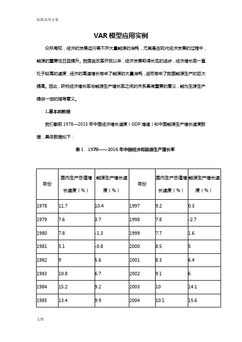
VAR模型应用实例众所周知,经济的发展运行离不开大量能源的消耗,尤其是在现代经济发展的过程中,能源的重要性日益提升。
我国自改革开放以来,经济发展取得长足的进步,经济增长率一直处于较高的速度,经济的高速增长带来了能源的大量消耗,进而带来了我国能源生产的巨大提高。
因此,研究经济增长率与能源生产增长率之间的关系具有重要的意义,能为生源生产提供一定的指导意义。
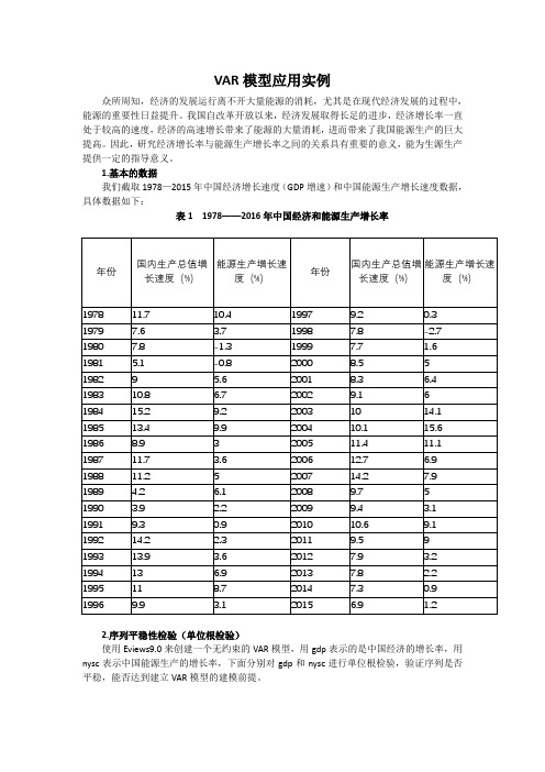
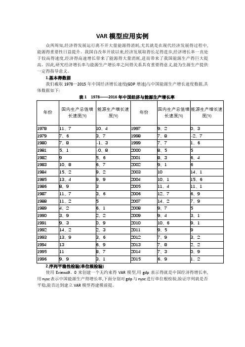
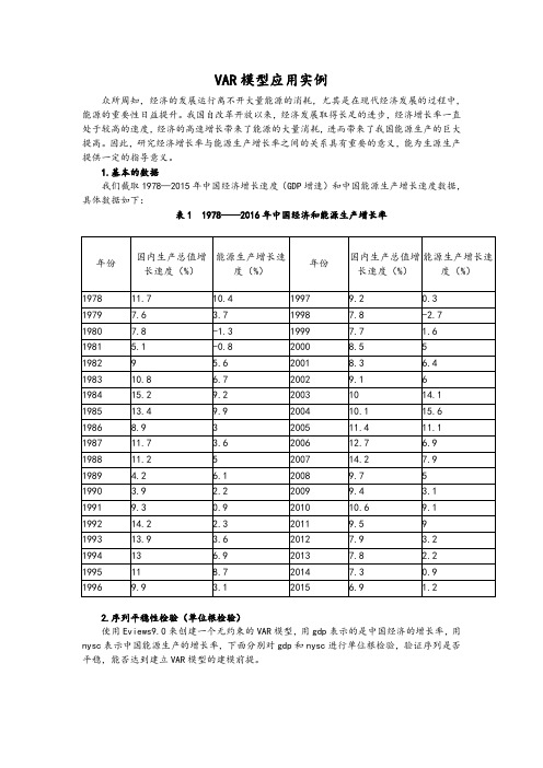
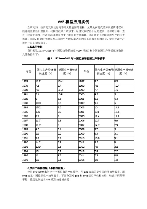
1.基本的数据我们截取1978—2015年中国经济增长速度(GDP增速)和中国能源生产增长速度数据,具体数据如下:表1 1978——2016年中国经济和能源生产增长率2.序列平稳性检验(单位根检验)使用Eviews9.0来创建一个无约束的VAR模型,用gdp表示的是中国经济的增长率,用nysc表示中国能源生产的增长率,下面分别对gdp和nysc进行单位根检验,验证序列是否平稳,能否达到建立VAR模型的建模前提。
图2.1 经济增速(GDP)的单位根检验图2.2 能源生产增速(nysc)的单位根检验经过检验,在1%的显著性水平上,gdp和nysc两个时间序列都是平稳的,符合建模的条件,我们建立一个无约束的VAR模型。
3.VAR模型的估计图3.1 模型的估计结果图3.2 模型的表达式4.模型的检验4.1模型的平稳性检验图4.1.1 AR根的表由图4.1.1知,AR所有单位根的模都是小于1的,因此估计的模型满足稳定性的条件。
图4.1.2 AR根的图通过对GDP增长率和能源生产增长率进进行了VAR模型估计,并采用AR根估计的方法对VAR模型估计的结果进行平稳性检验。
AR根估计是基于这样一种原理的:如果VAR模型所有根模的倒数都小于1,即都在单位圆内,则该模型是稳定的;如果VAR模型所有根模的倒数都大于1,即都在单位圆外,则该模型是不稳定的。
由图4.1.2可知,没有根是在单位圆之外的,估计的VAR模型满足稳定性的条件。
4.2 Granger因果检验图4.2.1 Granger因果检验结果图Granger因果检验的原假设是:H0:变量x不能Granger引起变量y备择假设是:H1:变量x能Granger引起变量y对VAR(2)进行Granger因果检验在1%的显著性水平之下,经济增速(GDP)能够Granger 引起能源生产增速(NYSC)的变化,即拒绝了原假设;同时,能源生产增速(NYSC)能够Granger经济增速(GDP)的变化,即拒绝了原假设,接受备择假设。
VAR模型应用案例完成

V A R模型应用案例完成 Document serial number【NL89WT-NY98YT-NC8CB-NNUUT-NUT108】VAR模型应用实例众所周知,经济的发展运行离不开大量能源的消耗,尤其是在现代经济发展的过程中,能源的重要性日益提升。
我国自改革开放以来,经济发展取得长足的进步,经济增长率一直处于较高的速度,经济的高速增长带来了能源的大量消耗,进而带来了我国能源生产的巨大提高。
因此,研究经济增长率与能源生产增长率之间的关系具有重要的意义,能为生源生产提供一定的指导意义。
1.基本的数据我们截取1978—2015年中国经济增长速度(GDP增速)和中国能源生产增长速度数据,具体数据如下:表1 1978——2016年中国经济和能源生产增长率使用来创建一个无约束的VAR模型,用gdp表示的是中国经济的增长率,用nysc表示中国能源生产的增长率,下面分别对gdp和nysc进行单位根检验,验证序列是否平稳,能否达到建立VAR模型的建模前提。
图经济增速(GDP)的单位根检验图能源生产增速(nysc)的单位根检验经过检验,在1%的显着性水平上,gdp和nysc两个时间序列都是平稳的,符合建模的条件,我们建立一个无约束的VAR模型。
3.VAR模型的估计图模型的估计结果图模型的表达式4.模型的检验模型的平稳性检验图 AR根的表由图知,AR所有单位根的模都是小于1的,因此估计的模型满足稳定性的条件。
图 AR根的图通过对GDP增长率和能源生产增长率进进行了VAR模型估计,并采用AR根估计的方法对VAR模型估计的结果进行平稳性检验。
AR根估计是基于这样一种原理的:如果VAR模型所有根模的倒数都小于1,即都在单位圆内,则该模型是稳定的;如果VAR模型所有根模的倒数都大于1,即都在单位圆外,则该模型是不稳定的。
由图可知,没有根是在单位圆之外的,估计的VAR模型满足稳定性的条件。
Granger因果检验图 Granger因果检验结果图Granger因果检验的原假设是:H:变量x不能Granger引起变量y备择假设是::变量x能Granger引起变量yH1对VAR(2)进行Granger因果检验在1%的显着性水平之下,经济增速(GDP)能够Granger引起能源生产增速(NYSC)的变化,即拒绝了原假设;同时,能源生产增速(NYSC)能够Granger经济增速(GDP)的变化,即拒绝了原假设,接受备择假设。
VAR示例

y1:钢材; y2:建材; y3:汽车; y4:机械; y5:家电
从第一个图中可以看出, 从第一个图中可以看出 , 当在本期给建材行业销售收入 一个正冲击后,钢材销售收入在前4期内小幅上下波动之后 一个正冲击后,钢材销售收入在前 期内小幅上下波动之后
(6 在第6期达到最高点 在第 期达到最高点( c12) =12.03,即在第 期y1对y2的响应是 期达到最高点 ,即在第6期 12.03) ;从第 期以后开始稳定增长。这表明建材行业受外 从第9期以后开始稳定增长 期以后开始稳定增长。
部条件的某一冲击后, 经市场传递给钢铁行业, 部条件的某一冲击后 , 经市场传递给钢铁行业 , 给钢铁行 业带来同向的冲击, 业带来同向的冲击 , 而且这一冲击具有显著的促进作用和 较长的持续效应。 较长的持续效应。 从第二幅图中可以看出, 从第二幅图中可以看出,当在本期给汽车行业销售收入 一个正冲击后,钢材销售收入在前5期内会上下波动 期内会上下波动; 一个正冲击后,钢材销售收入在前 期内会上下波动;从第 5期以后开始稳定增长 c13) =1.76)。这表明汽车行业的某一冲 期以后开始稳定增长( (5 期以后开始稳定增长 。 击也会给钢铁行业带来同向的冲击, 击也会给钢铁行业带来同向的冲击 , 即汽车行业销售收入 增加会在5个月后对钢材的销售收入产生稳定的拉动作用。 增加会在 个月后对钢材的销售收入产生稳定的拉动作用。 个月后对钢材的销售收入产生稳定的拉动作用
从第三幅图中可以看出, 从第三幅图中可以看出 , 机械行业销售收入的正冲击 经市场传递也会给钢材销售收入带来正面的影响, 经市场传递也会给钢材销售收入带来正面的影响 , 并且 此影响具有较长的持续效应。 此影响具有较长的持续效应 。 从第四幅图中可以看出当 在本期给家电行业销售收入一个正冲击后, 在本期给家电行业销售收入一个正冲击后 , 也会给钢材 销售收入带来正面的冲击,但是冲击幅度不是很大。 销售收入带来正面的冲击,但是冲击幅度不是很大。 综上所述,由于市场化程度、 综上所述,由于市场化程度、政府保护政策等各方面 的原因, 的原因 , 使得各下游相关行业的外部冲击会通过市场给 钢铁行业带来不同程度的影响, 但是都是同向的影响。 钢铁行业带来不同程度的影响 , 但是都是同向的影响 。 政府可以利用这种现象, 对市场进行有区别、 政府可以利用这种现象 , 对市场进行有区别 、 有重点的 调整,减少盲目的重复建设项目。 调整,减少盲目的重复关行业变化的响应
VAR模型应用案例 (完成)
VAR模型应用实例众所周知,经济得发展运行离不开大量能源得消耗,尤其就是在现代经济发展得过程中,能源得重要性日益提升。
我国自改革开放以来,经济发展取得长足得进步,经济增长率一直处于较高得速度,经济得高速增长带来了能源得大量消耗,进而带来了我国能源生产得巨大提高。
因此,研究经济增长率与能源生产增长率之间得关系具有重要得意义,能为生源生产提供一定得指导意义。
1.基本得数据我们截取1978—2015年中国经济增长速度(GDP增速)与中国能源生产增长速度数据,具体数据如下:表1 1978——2016年中国经济与能源生产增长率使用Eviews9、0来创建一个无约束得VAR模型,用gdp表示得就是中国经济得增长率,用nysc表示中国能源生产得增长率,下面分别对gdp与nysc进行单位根检验,验证序列就是否平稳,能否达到建立VAR模型得建模前提。
图2、1 经济增速(GDP)得单位根检验图2、2 能源生产增速(nysc)得单位根检验经过检验,在1%得显著性水平上,gdp与nysc两个时间序列都就是平稳得,符合建模得条件,我们建立一个无约束得VAR模型。
3.VAR模型得估计图3、1 模型得估计结果图3、2 模型得表达式4、模型得检验4、1模型得平稳性检验图4、1、1 AR根得表由图4、1、1知,AR所有单位根得模都就是小于1得,因此估计得模型满足稳定性得条件。
图4、1、2 AR根得图通过对GDP增长率与能源生产增长率进进行了VAR模型估计,并采用AR根估计得方法对VAR模型估计得结果进行平稳性检验。
AR根估计就是基于这样一种原理得:如果VAR模型所有根模得倒数都小于1,即都在单位圆内,则该模型就是稳定得;如果VAR模型所有根模得倒数都大于1,即都在单位圆外,则该模型就是不稳定得。
由图4、1、2可知,没有根就是在单位圆之外得,估计得VAR模型满足稳定性得条件。
4、2 Granger因果检验图4、2、1 Granger因果检验结果图Granger因果检验得原假设就是:H0:变量x不能Granger引起变量y备择假设就是:H1:变量x能Granger引起变量y对VAR(2)进行Granger因果检验在1%得显著性水平之下,经济增速(GDP)能够Granger引起能源生产增速(NYSC)得变化,即拒绝了原假设;同时,能源生产增速(NYSC)能够Granger经济增速(GDP)得变化,即拒绝了原假设,接受备择假设。
var模型r语言应用实例
var模型r语言应用实例引言在经济学和金融学领域,VAR(Vector Autoregression)模型是一种常用的时间序列分析方法。
VAR模型可以用于预测和分析多个相关变量之间的动态关系。
本文将介绍VAR模型的基本原理和在R语言中的应用实例。
一、VAR模型基本原理VAR模型是一种多元时间序列模型,它假设变量之间的关系是相互回应的,即每个变量的变化可以由其他变量的变化解释。
VAR模型的基本原理可以概括为以下几个步骤:1. 数据准备首先,需要收集和准备多个相关变量的时间序列数据。
这些变量应该是同一时间段内的观测值,例如每月的经济指标数据。
2. 检验时间序列的平稳性在进行VAR模型分析之前,需要对每个变量的时间序列进行平稳性检验。
平稳性是指时间序列的均值和方差在时间上保持不变的性质。
常用的平稳性检验方法包括ADF检验和单位根检验。
3. 确定VAR模型的滞后阶数滞后阶数是指VAR模型中所包含的时间滞后项的个数。
确定滞后阶数的方法有很多种,常用的方法包括信息准则(如AIC和BIC)和Ljung-Box检验。
4. 估计VAR模型参数估计VAR模型的参数可以使用最小二乘法或极大似然法。
在R语言中,可以使用vars包或vars::VAR函数进行参数估计。
在估计VAR模型参数之后,需要对模型进行诊断和检验。
常用的模型诊断方法包括残差平稳性检验、残差白噪声检验和模型拟合优度检验。
6. 模型预测和分析完成模型诊断和检验之后,可以使用VAR模型进行预测和分析。
VAR模型可以用于预测未来的变量值,同时还可以分析变量之间的动态关系和冲击响应。
二、R语言中的VAR模型应用实例下面将通过一个实例来演示在R语言中如何应用VAR模型进行分析和预测。
1. 数据准备首先,我们需要准备多个相关变量的时间序列数据。
以宏观经济领域为例,我们可以选择GDP、通货膨胀率和利率作为研究对象。
假设我们收集了这三个变量的季度数据。
2. 检验时间序列的平稳性使用adf.test函数对每个变量的时间序列进行平稳性检验。
var模型r语言应用实例
var模型r语言应用实例VAR模型是一种常用的时间序列分析方法,可以用来分析多个变量之间的相互关系。
R语言是一个功能强大的统计分析工具,可以用来实现VAR模型的建模和预测。
下面是一个VAR模型在R语言中的应用实例:假设我们有两个变量X和Y,它们之间存在某种关系。
我们可以使用VAR模型来建立它们之间的关系模型。
首先,我们需要导入数据并将其转换为时间序列对象:```R# 导入数据data <- read.csv('data.csv')# 转换为时间序列对象ts_data <- ts(data[,c('X','Y')], start=1, end=100, frequency=1)```然后,我们可以使用vars包中的VAR函数来建立VAR模型:```R# 导入vars包library(vars)# 建立VAR模型model <- VAR(ts_data, p=2)```在这个例子中,我们使用了滞后阶数p=2,这意味着我们考虑了前两个时期的影响。
接下来,我们可以使用predict函数来预测未来的值:```R# 预测未来10期的值forecast <- predict(model, n.ahead=10)```最后,我们可以使用plot函数来可视化预测结果:```R# 可视化预测结果plot(forecast)```以上就是一个简单的VAR模型在R语言中的应用实例。
通过VAR 模型,我们可以更好地理解多个变量之间的相互关系,并进行未来值的预测。
VAR模型应用案例 (完成)
标准实用文案文档VAR模型应用实例众所周知,经济的发展运行离不开大量能源的消耗,尤其是在现代经济发展的过程中,能源的重要性日益提升。
我国自改革开放以来,经济发展取得长足的进步,经济增长率一直处于较高的速度,经济的高速增长带来了能源的大量消耗,进而带来了我国能源生产的巨大提高。
因此,研究经济增长率与能源生产增长率之间的关系具有重要的意义,能为生源生产提供一定的指导意义。
1.基本的数据我们截取1978—2015年中国经济增长速度(GDP增速)和中国能源生产增长速度数据,具体数据如下:表1 1978——2016年中国经济和能源生产增长率2.序列平稳性检验(单位根检验)使用Eviews9.0来创建一个无约束的VAR模型,用gdp表示的是中国经济的增长率,用nysc表示中国能源生产的增长率,下面分别对gdp和nysc进行单位根检验,验证序列是否平稳,能否达到建立VAR模型的建模前提。
图2.1 经济增速(GDP)的单位根检验图2.2 能源生产增速(nysc)的单位根检验经过检验,在1%的显著性水平上,gdp和nysc两个时间序列都是平稳的,符合建模的条件,我们建立一个无约束的VAR模型。
3.VAR模型的估计图3.1 模型的估计结果图3.2 模型的表达式4.模型的检验4.1模型的平稳性检验图4.1.1 AR根的表由图4.1.1知,AR所有单位根的模都是小于1的,因此估计的模型满足稳定性的条件。
图4.1.2 AR根的图通过对GDP增长率和能源生产增长率进进行了VAR模型估计,并采用AR根估计的方法对VAR模型估计的结果进行平稳性检验。
AR根估计是基于这样一种原理的:如果VAR模型所有根模的倒数都小于1,即都在单位圆内,则该模型是稳定的;如果VAR模型所有根模的倒数都大于1,即都在单位圆外,则该模型是不稳定的。
由图4.1.2可知,没有根是在单位圆之外的,估计的VAR模型满足稳定性的条件。
4.2 Granger因果检验图4.2.1 Granger因果检验结果图Granger因果检验的原假设是:H0:变量x不能Granger引起变量y备择假设是:H1:变量x能Granger引起变量y对VAR(2)进行Granger因果检验在1%的显著性水平之下,经济增速(GDP)能够Granger引起能源生产增速(NYSC)的变化,即拒绝了原假设;同时,能源生产增速(NYSC)能够Granger经济增速(GDP)的变化,即拒绝了原假设,接受备择假设。
VAR模型的应用案例 (完成)
VAR模型应用实例众所周知,经济的发展运行离不开大量能源的消耗,尤其是在现代经济发展的过程中,能源的重要性日益提升。
我国自改革开放以来,经济发展取得长足的进步,经济增长率一直处于较高的速度,经济的高速增长带来了能源的大量消耗,进而带来了我国能源生产的巨大提高。
因此,研究经济增长率与能源生产增长率之间的关系具有重要的意义,能为生源生产提供一定的指导意义。
1.基本的数据我们截取1978—2015年中国经济增长速度(GDP增速)和中国能源生产增长速度数据,具体数据如下:表1 1978——2016年中国经济和能源生产增长率2.序列平稳性检验(单位根检验)使用Eviews9.0来创建一个无约束的VAR模型,用gdp表示的是中国经济的增长率,用nysc表示中国能源生产的增长率,下面分别对gdp和nysc进行单位根检验,验证序列是否平稳,能否达到建立VAR模型的建模前提。
图2.1 经济增速(GDP)的单位根检验图2.2 能源生产增速(nysc)的单位根检验经过检验,在1%的显著性水平上,gdp和nysc两个时间序列都是平稳的,符合建模的条件,我们建立一个无约束的VAR模型。
3.VAR模型的估计图3.1 模型的估计结果图3.2 模型的表达式4.模型的检验4.1模型的平稳性检验图4.1.1 AR根的表由图4.1.1知,AR所有单位根的模都是小于1的,因此估计的模型满足稳定性的条件。
图4.1.2 AR根的图通过对GDP增长率和能源生产增长率进进行了VAR模型估计,并采用AR根估计的方法对VAR模型估计的结果进行平稳性检验。
AR根估计是基于这样一种原理的:如果VAR模型所有根模的倒数都小于1,即都在单位圆内,则该模型是稳定的;如果VAR模型所有根模的倒数都大于1,即都在单位圆外,则该模型是不稳定的。
由图4.1.2可知,没有根是在单位圆之外的,估计的VAR模型满足稳定性的条件。
4.2 Granger因果检验图4.2.1 Granger因果检验结果图Granger因果检验的原假设是:H0:变量x不能Granger引起变量y备择假设是:H1:变量x能Granger引起变量y对VAR(2)进行Granger因果检验在1%的显著性水平之下,经济增速(GDP)能够Granger 引起能源生产增速(NYSC)的变化,即拒绝了原假设;同时,能源生产增速(NYSC)能够Granger经济增速(GDP)的变化,即拒绝了原假设,接受备择假设。
VAR模型应用案例解析(完成)

VAR模型应用实例众所周知,经济的发展运行离不开大量能源的消耗,尤其是在现代经济发展的过程中,能源的重要性日益提升。
我国自改革开放以来,经济发展取得长足的进步,经济增长率一直处于较高的速度,经济的高速增长带来了能源的大量消耗,进而带来了我国能源生产的巨大提高。
因此,研究经济增长率与能源生产增长率之间的关系具有重要的意义,能为生源生产提供一定的指导意义。
1.基本的数据我们截取1978—2015年中国经济增长速度(GDP增速)和中国能源生产增长速度数据,具体数据如下:表1 1978——2016年中国经济和能源生产增长率2.序列平稳性检验(单位根检验)使用Eviews9.0来创建一个无约束的VAR模型,用gdp表示的是中国经济的增长率,用nysc表示中国能源生产的增长率,下面分别对gdp和nysc进行单位根检验,验证序列是否平稳,能否达到建立VAR模型的建模前提。
图2.1 经济增速(GDP)的单位根检验图2.2 能源生产增速(nysc)的单位根检验经过检验,在1%的显著性水平上,gdp和nysc两个时间序列都是平稳的,符合建模的条件,我们建立一个无约束的VAR模型。
3.VAR模型的估计图3.1 模型的估计结果图3.2 模型的表达式4.模型的检验4.1模型的平稳性检验图4.1.1 AR根的表由图4.1.1知,AR所有单位根的模都是小于1的,因此估计的模型满足稳定性的条件。
图4.1.2 AR根的图通过对GDP增长率和能源生产增长率进进行了VAR模型估计,并采用AR根估计的方法对VAR模型估计的结果进行平稳性检验。
AR根估计是基于这样一种原理的:如果VAR模型所有根模的倒数都小于1,即都在单位圆内,则该模型是稳定的;如果VAR模型所有根模的倒数都大于1,即都在单位圆外,则该模型是不稳定的。
由图4.1.2可知,没有根是在单位圆之外的,估计的VAR模型满足稳定性的条件。
4.2 Granger因果检验图4.2.1 Granger因果检验结果图Granger因果检验的原假设是:H0:变量x不能Granger引起变量y备择假设是:H1:变量x能Granger引起变量y对VAR(2)进行Granger因果检验在1%的显著性水平之下,经济增速(GDP)能够Granger 引起能源生产增速(NYSC)的变化,即拒绝了原假设;同时,能源生产增速(NYSC)能够Granger经济增速(GDP)的变化,即拒绝了原假设,接受备择假设。
VAR模型应用案例
VAR模型应用案例A VAR model is popular in many areas of economics, including finance, macroeconomics, and international economics. In finance, the VAR model is used for portfolio management, asset pricing, and risk management. In macroeconomics, the VAR model is used to analyse the relationship between economic variables, such as GDP, inflation, and employment. In international economics, the VAR model is used to study the relationship between countries and their economies.The VAR model can also be used to analyse and forecast the effects of policy changes. For example, if a government implements a policy to reduce the unemployment rate, the VAR model can be used to analyse how this might affect inflation.This can help policymakers understand the implications of their policy decisions and better prepare for the economic consequences.VAR models can also be used to analyse how economicconditions in one part of the world affect economic conditionsin other parts of the world. For example, if the economy ofJapan is in recession, a VAR model can be used to analyse howthis might affect the economies of other countries, such asChina and the United States. This can help economists understand the implications of global economic conditions and betterprepare for their economic consequences.In addition to economic analysis, VAR models can also be used in forecasting. For example, they can be used to forecast the effects of different policy changes or to predict the future state of the economy. This can help policymakers make more informed decisions based on the most accurate predictions.。
VAR模型应用案例 (完成)
欢迎共阅VAR模型应用实例众所周知,经济的发展运行离不开大量能源的消耗,尤其是在现代经济发展的过程中,能源的重要性日益提升。
我国自改革开放以来,经济发展取得长足的进步,经济增长率一直处于较高的速度,经济的高速增长带来了能源的大量消耗,进而带来了我国能源生产的巨大提高。
因此,研究经济增长率与能源生产增长率之间的关系具有重要的意义,能为生源生产提供一定的指导意义。
1.基本的数据原假设是:H0:变量x不能Granger引起变量y备择假设是:H1:变量x能Granger引起变量y对VAR(2)进行Granger因果检验在1%的显着性水平之下,经济增速(GDP)能够Granger引起能源生产增速(NYSC)的变化,即拒绝了原假设;同时,能源生产增速(NYSC)能够Granger经济增速(GDP)的变化,即拒绝了原假设,接受备择假设。
5滞后期长度图5.1 VAR模型滞后期选择结果从上图可以看出LR, FPE, AIC, SC, HQ都指向同样的2阶滞后期,因此应该选择VAR(2)进行后续的分析。
6.脉冲函数图6.1 各因素脉冲响应函数结果图从图6.1可以看出:经济增长率(GDP)和能源生产(NYSC)各自对于自身的冲击,在前四期是快速下降的趋势,并且出现负值的情况。
但是,GDP增速的变化基本上在第七期就保持了持平的一个状况;而能源生产(NYSC)的变化是在第九期的时候实现持平的状态。
这需要政府和市场共同的努力,政府应该做好服务角色,为能源生产市场提供良好的服务,保障市场公平,完善相关的产业政策,提供良好的环境。
市场应该公开公正的竞争,不断引进新技术,提高能源的生产效率,为经济的健康发展提供动力基础。
VAR模型应用案例 (完成)
VAR模型应用实例众所周知,经济的发展运行离不开大量能源的消耗,尤其是在现代经济发展的过程中,能源的重要性日益提升。
我国自改革开放以来,经济发展取得长足的进步,经济增长率一直处于较高的速度,经济的高速增长带来了能源的大量消耗,进而带来了我国能源生产的巨大提高。
因此,研究经济增长率与能源生产增长率之间的关系具有重要的意义,能为生源生产提供一定的指导意义。
1.基本的数据我们截取1978—2015年中国经济增长速度(GDP增速)和中国能源生产增长速度数据,具体数据如下:表1 1978——2016年中国经济和能源生产增长率2.序列平稳性检验(单位根检验)使用Eviews9.0来创建一个无约束的VAR模型,用gdp表示的是中国经济的增长率,用nysc表示中国能源生产的增长率,下面分别对gdp和nysc进行单位根检验,验证序列是否平稳,能否达到建立VAR模型的建模前提。
图2.1 经济增速(GDP)的单位根检验图2.2 能源生产增速(nysc)的单位根检验经过检验,在1%的显著性水平上,gdp和nysc两个时间序列都是平稳的,符合建模的条件,我们建立一个无约束的VAR模型。
3.VAR模型的估计图3.1 模型的估计结果图3.2 模型的表达式4.模型的检验4.1模型的平稳性检验图4.1.1 AR根的表由图4.1.1知,AR所有单位根的模都是小于1的,因此估计的模型满足稳定性的条件。
图4.1.2 AR根的图通过对GDP增长率和能源生产增长率进进行了VAR模型估计,并采用AR根估计的方法对VAR模型估计的结果进行平稳性检验。
AR根估计是基于这样一种原理的:如果VAR模型所有根模的倒数都小于1,即都在单位圆内,则该模型是稳定的;如果VAR模型所有根模的倒数都大于1,即都在单位圆外,则该模型是不稳定的。
由图4.1.2可知,没有根是在单位圆之外的,估计的VAR模型满足稳定性的条件。
4.2 Granger因果检验图4.2.1 Granger因果检验结果图Granger因果检验的原假设是:H0:变量x不能Granger引起变量y备择假设是:H1:变量x能Granger引起变量y对VAR(2)进行Granger因果检验在1%的显著性水平之下,经济增速(GDP)能够Granger 引起能源生产增速(NYSC)的变化,即拒绝了原假设;同时,能源生产增速(NYSC)能够Granger经济增速(GDP)的变化,即拒绝了原假设,接受备择假设。
向量自回归var模型案例附数据
向量自回归var模型案例附数据向量自回归VAR模型案例附数据向量自回归(Vector Autoregression, VAR)模型是一种广泛应用于多元时间序列分析的模型框架。
VAR模型可以同时对多个相互关联的时间序列变量进行建模,捕捉它们之间的动态关系。
以下是一个VAR模型的案例,并附有相关的数据。
案例背景:假设我们有三个相互关联的时间序列变量:GDP增长率(gdp)、通货膨胀率(infl)和利率(interest)。
我们希望利用VAR模型来分析这三个变量之间的动态关系,并对它们进行预测。
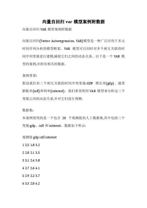
数据集:本案例使用的是一个包含20个观测值的人工数据集,其中包括三个变量:gdp、infl和interest。
数据如下所示:观测值 gdp infl interest1 2.5 1.8 3.22 2.8 2.1 3.53 3.1 2.4 3.84 2.7 2.6 4.15 2.9 2.2 3.76 3.3 2.8 4.27 3.5 3.1 4.58 3.2 2.9 4.39 3.6 3.3 4.710 3.8 3.5 5.111 3.4 3.2 4.612 3.6 3.4 4.813 4.1 3.7 5.314 4.3 4.1 5.715 4.5 4.3 6.116 4.2 4.5 5.917 4.4 4.2 6.218 4.7 4.6 6.519 4.9 4.8 6.720 5.1 5.2 7.1在这个案例中,我们可以构建一个VAR模型,将gdp、infl和interest 作为内生变量,并估计它们之间的动态关系。
通过对模型进行诊断和评估,我们可以了解这三个变量之间的相互影响,并基于模型对未来的GDP增长率、通货膨胀率和利率进行预测。
VaR计量模型分析案例
pt 是 t 日上证综合指数的收盘价格。以下模型中的参数估计均是用 SAS6.12 统计软件实现
的。 如图 1 所示,上证综合指数收益率集中在(-0.05,0.05)之间,在波动较大的几个时段 上收益率绝对值的峰值达到了 0.1,在到达顶峰后又迅速回落。在样本期间,平均收益率为 0.00284,偏度为-0.256529,峰度为 9.401051,数据分布向左偏移,有一个沉重的尾巴。这 说明从整体上看,收益率低于其均值的时候较多,波动性强,尾部和中间包含了大量的统计 信息。J-B 正态性检验得到的统计量值为 2558.392,也说明收益率序列显著异于正态分布。
检验说明直到高阶收益率序列仍然存在着强烈的异方差性, 用ENGARCH模型族来拟合 数据是合理的。随后用Augument-Dikey Fuller方法对收益率进行单位根检验,得到的ADF值 拒绝了单位根的假设,序列是平稳的。 对序列 {rt }进行了自相关和偏自相关的检验后,我们选用的均值模型为:
rt = c + ϕrt −12 + ρ rt −15 + δ ht + ε t
这里的 Γ(• ) 是 GAMMA 函数,v 是自由度。似然函数可通过对偶牛顿算法或信赖域算 法极大化得到。 由于股市收益率的波动回随信息的变化而出现非对称性的特点, 利空消息引 起的波动一般更大,为了刻画波动的非对称性,Nelson 等人提出了非对称性(Asymmetric) GARCH 模型,包括 EGARCH 及 TGARCH 等模型。 在 EGARCH 模型中,条件方差 ht 为延迟扰乱 ε t −i 的反对称函数:
ORDER 1 2 3 4 5 6 Q 73.8759 118.067 147.268 166.016 171.458 183.292 Prob>Q 0.0001 0.0001 0.0001 0.0001 0.0001 0.0001 LM 71.9199 94.3105 103.077 106.446 106.448 109.604 Prob>LM 0.0001 0.0001 0.0001 0.0001 0.0001 0.0001 ORDER 7 8 9 10 11 12 Q 189.701 192.070 194.180 200.472 207.641 208.600 Prob>Q 0.0001 0.0001 0.0001 0.0001 0.0001 0.0001 LM 110.049 110.074 110.101 112.086 114.006 114.455 Prob>LM 0.0001 0.0001 0.0001 0.0001 0.0001 0.0001
风险管理中的统计学模型与应用案例
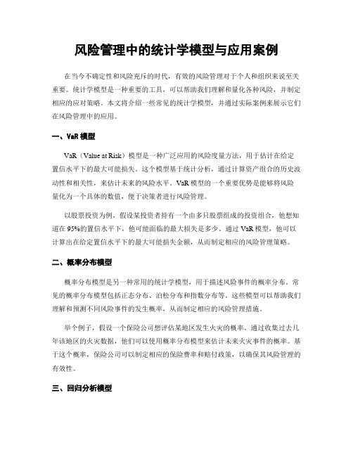
风险管理中的统计学模型与应用案例在当今不确定性和风险充斥的时代,有效的风险管理对于个人和组织来说至关重要。
统计学模型是一种重要的工具,可以帮助我们理解和量化各种风险,并制定相应的应对策略。
本文将介绍一些常见的统计学模型,并通过实际案例来展示它们在风险管理中的应用。
一、VaR模型VaR(Value at Risk)模型是一种广泛应用的风险度量方法,用于估计在给定置信水平下的最大可能损失。
这个模型基于统计分析,通过计算资产组合的历史波动性和相关性,来估计未来的风险水平。
VaR模型的一个重要优势是能够将风险量化为一个具体的数值,便于决策者进行风险管理。
以股票投资为例,假设某投资者持有一个由多只股票组成的投资组合,他想知道在95%的置信水平下,他可能面临的最大损失是多少。
通过VaR模型,他可以计算出在给定置信水平下的最大可能损失金额,从而制定相应的风险管理策略。
二、概率分布模型概率分布模型是另一种常用的统计学模型,用于描述风险事件的概率分布。
常见的概率分布模型包括正态分布、泊松分布和指数分布等。
这些模型可以帮助我们理解和预测不同风险事件的发生概率,从而制定相应的风险管理措施。
举个例子,假设一个保险公司想评估某地区发生火灾的概率。
通过收集过去几年该地区的火灾数据,他们可以使用概率分布模型来估计未来火灾事件的概率。
基于这个概率,保险公司可以制定相应的保险费率和赔付政策,以确保其风险管理的有效性。
三、回归分析模型回归分析模型是一种用于探索和预测变量之间关系的统计学模型。
在风险管理中,回归分析模型可以帮助我们理解和量化不同变量对风险的影响程度,从而制定相应的风险管理策略。
以金融领域为例,假设一个银行想评估贷款违约的可能性与借款人的收入、信用评级和负债水平之间的关系。
通过回归分析模型,银行可以确定不同变量对贷款违约的影响程度,并据此制定相应的风险管理政策,如调整贷款利率或要求更严格的信用评级。
四、蒙特卡洛模拟蒙特卡洛模拟是一种基于概率统计的模型,用于模拟和分析不确定性事件的可能结果。
向量自回归var模型案例附数据
向量自回归var模型案例附数据向量自回归VAR模型案例附数据向量自回归(Vector Autoregression, VAR)模型是一种广泛应用于多元时间序列分析的建模方法。
这种模型将每个内生变量作为其自身滞后值和所有其他内生变量的滞后值的线性函数进行描述。
VAR模型具有简单、灵活和易于推广的优点,因此在宏观经济分析、金融数据分析等领域得到了广泛应用。
以下是一个基于R语言对VAR模型进行估计和预测的案例示例,数据来自于加拿大的一些宏观经济变量:数据说明:变量包括加拿大的实际GDP(rgdp)、GDP平减指数(deflator)、实际进口量(im)和实际出口量(ex),时间范围为1981年第1季度到2001年第2季度,共81个观测值。
```r# 导入数据canadata <- read.table("canadata.txt", header = TRUE)str(canadata)# 对数据取对数并构造时间序列对象y <- log(canadata[, 2:5])z <- ts(y, start = c(1981, 1), frequency = 4)# 估计VAR模型library(vars)var.model <- VAR(z, p = 2, type = "const")summary(var.model)# 预测fcast <- predict(var.model, n.ahead = 8)# 数据可视化plot(fcast$fcst[, 1], type = 'l', ylim = range(z[, 1], fcast$fcst[, 1]), xlab = "Time", ylab = "rgdp", main = "Canadian GDP Forecast")lines(z[, 1], col = "blue")```。
VAR模型应用案例
VAR模型应用案例
一、背景
随着现代经济的发展,多元化的外汇投资已经成为企业和金融机构寻求利润增长的重要方式。
有关外汇投资领域的研究越来越重视外汇市场经济环境变量和多元组合投资的影响。
其中,多元组合投资可以充分利用经济环境变量对外汇汇率的影响,以更好地实现风险控制的目的。
基于该概念,有很多研究开发出了基于前沿的时变多元组合投资模型,其中VAR模型是最重要的模型之一
二、VAR模型的概述
运动变量分析(VAR)模型是有关金融时间序列分析的一种经典方法。
它是通过线性回归分析,来探索多变量之间的线性关系,以及它们对于其他变量均衡状态的影响,从而有效地捕获金融市场的变换动态,更好地掌握金融风险暴露量,并针对其进行风险管理。
三、VAR模型在外汇投资领域的应用
众所周知,外汇市场是最具挑战性和复杂性的投资市场之一,因此利用VAR模型来实现外汇投资是可行的。
- 1、下载文档前请自行甄别文档内容的完整性,平台不提供额外的编辑、内容补充、找答案等附加服务。
- 2、"仅部分预览"的文档,不可在线预览部分如存在完整性等问题,可反馈申请退款(可完整预览的文档不适用该条件!)。
- 3、如文档侵犯您的权益,请联系客服反馈,我们会尽快为您处理(人工客服工作时间:9:00-18:30)。
VAR模型应用实例众所周知,经济的发展运行离不开大量能源的消耗,尤其是在现代经济发展的过程中,能源的重要性日益提升。
我国自改革开放以来,经济发展取得长足的进步,经济增长率一直处于较高的速度,经济的高速增长带来了能源的大量消耗,进而带来了我国能源生产的巨大提高。
因此,研究经济增长率与能源生产增长率之间的关系具有重要的意义,能为生源生产提供一定的指导意义。
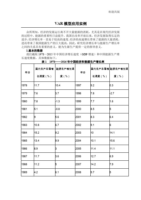
1•基本的数据我们截取1978—2015年中国经济增长速度(GDP增速)和中国能源生产增长速度数据,具体数据如下:表1 1978―― 2016年中国经济和能源生产增长率2•序列平稳性检验(单位根检验)使用Eviews9.0来创建一个无约束的VAR模型,用gdp表示的是中国经济的增长率,用nysc表示中国能源生产的增长率,下面分别对gdp和nysc进行单位根检验,验证序列是否平稳,能否达到建立VAR模型的建模前提。
Augm&nted Di ckey-Fuller Test EquationDependent Variables (GDP) Method. Least Squares Date: 05/17/17 Time: 10:55 Sample (adjusted): 19S2 2015Included observations: 34 after adjustmentsVariable Coefficient St! Error t^Statistic Prob.GDP(-1)-0.8561710.221114 -18675530,0006EXGDPHJ)0.6256310.193529 3.23275510031D(GDP 図)0.0492400.175617 0.280544 07811D(GDP(-3))0264937 0.16734B 1.583145 01242 C3540050 2222961 3,841745 00006R-squareri 0.45S475 Mean dependent var 0.052941Adjusted R-squared 0 383782 S.D d即巴口血吋调「 2.545731r r di “內erm 洽占耗…甘尺讨丹, A图2.1经济增速(GDP)的单位根检验0 Series: NYSC Workfilm : UNTirLED!:Jntitled\P BI-V ——JilMM-ywMqVievy P IXK Object Properties Print I Pk me Freeze Scimple Genr Sheet Graph图22能源生产增速(nysc )的单位根检验经过检验,在1%的显著性水平上,gdp 和nysc 两个时间序列都是平稳的,符合建模的 条件,我们建立一个无约束的 VAR 模型。
3.VAR 模型的估计Augmented Dickey-Full er Unit Root Test on MYSChull Hypothesis: NYSC has a unit rootDwg&nous; ConstantLag Length: 1 fAutomatic- based on SIC,rnaj (lag=9)t-Statistic Prob *AUQniMt£(1 Die 魁y-FUll 总「tests 情t 圖 t -3.935987 (LQD4弓S%kvel -2 945S42 10% level-2.611531* MacKinnon (1996) one-sided f>valjes.Augrnented Dicke ?-FullerTest Equation Dependent Variable: D(NYSC) Method: Least Squares Date: 05/17/17 Tine: 10:59 Sample [adjusted); 1930 2015Included observations: 36 after adjustm&ntsVariable Co efficient Std Error 1-8! ati sticProb. hYSCM) -0 530986 0 134905 -3935987 0 0004 D[N¥SC(-1»0 430549 0.150055 2 922585 0 0062 C 2 7469380 05726612043000 0030R-squared0 34306B Main dependentvar -0 069444 .Adjusted R-squared 0.303254 S D dependent war 3.610704 S.E. of regression 2 930431 Akaike info criterion 5067831 Sum squared resid 283.3851 Schwarz criterion 5.199791 Log likelihood -88.22096 Hannan-Quinn criter. 5.113889 F-statistic 8.&16746 Durbin-Wstsor stat 1.990251ProLiF-slatiStic)0.000975Ve dor Autor&gression EstimatesDate: 05/17/17 Time: 11:03Sample (adjusted)' 1980 2015IndLided oDserations: 36 after adjustmEnts Standarfl errors in() & 卜statistics in[]GDP NYSCGDP[-1)0.B25644(0.16499>[5.003B9)0271538(0.23569)[1.15068]GDP 卜2)-0.530495(015625)[-3.19096]-0 292356 (0 237601 [^1 22942]NYSC{-1^-0.052225(0.11565)F045156]0.S4-6355 (0.16542: [511612]NYSC(-2)0.1&6100(0.11349> H63977]-0.35756a [0.16234) 1-220263]G 6.194513C1.50887>14.10539' 2 353291 (2.15827} [1.32665]R-squared 0.492565 9554387Adj. R-squared 0.427089 0.4&B 朋9Sum sq. res id合1305151 267.0323S E equation 2.051969 2934965F-statistic Z522S90 9,641791Log likelihood-74,26525-87.15117Altai kreAIC 4.403525 5119509 Schwarz SC 4.S23558 5339442Mean dependent 9.7380695016667S D deperdent 2.710&54 4137805Determinant res id covariance (doradj.) 30.72390 Determinant res id covariance22.78215L OQ likelihood -15B4312Altai Ice information crit&rior 9357287Schwa IT criterion 9 797154图3.1模型的估计结果回LS i 2 cap iiirscTO Milftl ;GDP = c(t L )*^Df (-1) + C (t2)^CDP (-2)C (L 3>KY£C(-1) + C (L 4)*infSC (-2) + C(LE )1IY5C = Ct2.1)*CDP (-1^ + CC2」2)*GDP (-2)+ 匚仅「引*耽既(-1) ■+ C (2, 4)*HVEC (-2) +匸化为 1TAL Medal - Svlrititut«d C»«££ivivntiGKP = fl. 3E55U312B35*^Jf (-1) - 0. 53Q434 ?Q?4S4**?®r(-£} - Q, 05E2E47^H )2 引T SC(-l) + □. lBGl00400721WSC (-E )+ 6.19451B^4763ifYSC = 0.271567998674*GD I PC-1) - 0. 232356168154*GDPt-2)0 84^35506574?^fflSCH) - 0. 35r567G3E 748*]JV5C (-£) + 2 363E9KJ617S图3.2 模型的表达式4•模型的检验 4.1模型的平稳性检验回 Var: UNTITLED V/orkfile : UNTITLED::UntitledRoots at Characteristic Polynomial Endaflenous variaMes: GDPNYSG Exogenous variables' C Lag specification: 1 2Date: 05/17/17 Time. 11:11RootModulus0.5&60S6 ” 0.4517091 0 724220 0.5&60S5 + 0 451708i 0.724220 0.2&9664 - 0.5265511 0.6321 眈 0.2&9S64 + 0 626551i0.682196No root lies outside the unit circle.VAR s artisfies the statMlit^ cand itio n图4.1.1 AR 根的表由图4.1.1知,AR 所有单位根的模都是小于 1的,因此估计的模型满足稳定性的条件。
图4.1.2 AR根的图通过对GDP增长率和能源生产增长率进进行了VAR模型估计,并采用AR根估计的方法对VAR模型估计的结果进行平稳性检验。
AR根估计是基于这样一种原理的:如果VAR模型所有根模的倒数都小于1,即都在单位圆内,则该模型是稳定的;如果VAR模型所有根模的倒数都大于1,即都在单位圆外,则该模型是不稳定的。