信号与系统英文课件chapter 4
奥本海姆版信号与系统ppt
+
Energy : t1 t t2
2
1
shift
f (t )
2 1
1 t
2
2
0
Scaling
Scaling
2
reversal
t
f (t )
2 1
shift
2 1
f (1 t )
f (1 3t )
1
t
0 1
1 0
1
2
2
1
0 1
t
1
2
1 3
0 2
t
3
f (3t )
f (1 3t )
Scaling
1
1 3
2
shift
1.2 Transformation of the Independent Variable
1.2.1 Examples of Transformations 1. Time Shift x(t-t0), x[n-n0]
t0<0
Advance
Time Shift
n0>0
Delay
x(t) and x(t-t0), or x[n] and x[n-n0]:
2. Time Reversal x(-t), x[-n]
——Reflection of x(t) or x[n]
2. Time Reversal x(-t), x[-n]
【医学英文课件】 《生物医学信号处理(双语)》精品课件
另外注意连续时间和离散时间的傅里叶变换是否具有 周期性: X(ejω)具有周期性, 周期2π。X(jω)不具有周期性。
9
连续时间傅里叶变换和离散时间傅里叶变换间的联系
奥本海姆《 信号与系统》在 “第7章 采样”的“7.4 Discrete-Time Processing of Continuous-time Signals”一 节中, 因对连续时间信号xc(t)进行采样(得到xd[n]), 在分 析频谱时需要同时涉及到连续时间信号的傅里叶变换和
Time Signal
2
4.0 Introduction
➢Continuous-time signal processing can be implemented through a process of sampling, discrete-time processing, and the subsequent reconstruction of a continuous-time signal.
ifs a m p lin g p e r io d T 1 6 0 0 0 .
Solution:
x n x c n T c o s 4 0 0 0 T n c o s 2 3 n c o s w 0 n
T h e h i g h e s tf r e q u e n c y o ft h e s i g n a l : 0 4 0 0 0
8
连续时间傅里叶变换和离散时间傅里叶变换间的联系
在奥本海姆的《信号与系统》教材里, 在 “第7章 采样”
内容之前,连续时间傅里叶变换X(jω), 和离散时间傅里
叶变换X(ejω)中涉及的频率都用相同的频率符号ω表示,
没有加以区分, 各说各话。
Chapter1 Signals and Systems
Example Fig 3
1.2 Transformations of The independent Variable
1.2.3 Even and Odd Signals
1.2 Transformations of The indepenຫໍສະໝຸດ ent Variable2
The total energy over an infinite time interval in discrete-time is defined as:
E lim
N n N
| x[n] |
2
N
n
| x[n] |2
1.1 Continuous-time and Discretetime Signals
Preface
◆Chapter1
Signals and Systems
◆ Chapter2
◆ Chapter3
Linear Time-invariant Systems
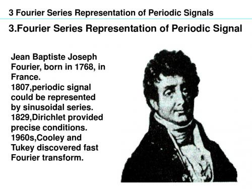
Fourier Series representation of periodic
signals
◆ Chapter4 ◆ Chapter5
Sinusoidal Signals(正弦信号):
1.3 Exponential And Sinusoidal Signals
1.3.1 Continuous-time Complex Exponential and Sinusoidal Signals
Sinusoidal Signals(正弦信号):
1 [ n] 0 n0 n0
1
[n]
2
《信号与系统》第十章课件(英文版)

9The z-transform reduces to the Fourier transform for values of z Unit circle on the unit circle.
Im z=ejω
z-plane
ω
1
Re
5
Sichuan University <Signals and Systems> Ch 10 The z-Transform
Example 10.3 Consider a signal that is the sum of two real
exponentials: x[n] = 7⎜⎛ 1 ⎟⎞ n u[n] − 6⎜⎛ 1 ⎟⎞ n u[n].
⎝3⎠
⎝2⎠
The z-transform is then
∑ ∑ X ( z) = 7 +∞ ⎜⎛ 1 ⎟⎞n u[n]z −n − 6 +∞ ⎜⎛ 1 ⎟⎞ n u[n]z −n
z z-transform expand the application in which Fourier analysis can be used.
2
Sichuan University <Signals and Systems> Ch 10 The z-Transform
10.1 The z-Transform
Transform 2. The Inverse z-Transform 3. Geometric Evaluation of the Fourier Transform from the Pole-
Zero Plot 4. Properties of the z-Transform and some Common z-Transform
信号与系统课件
● Examples
x(t) 1 -2 -1 0 -1 1 2 t -1 1 0 -1 1 2 3 4 t -3 -2 -1 y(t) = x(t-2) y(t) = x(t+1) 1 0 -1 1 t
Original Signal
ENEL 341– Signals and Transforms
Delayed Signal
● There are two types of transformations − Time transformations : apply a mathematical transformation on the time (the horizontal or time axis)
1. Time Reversal 2. Time Scaling 3. Time Shifting
x(t) 1 -1 0 1 -1 2 t -1 y(t) = 2.x(t) 2 1 0 1 -1 -2 2 t
Original Signal Signal after Amplitude Scaling
12
ENEL 341– Signals and Transforms
Amplitude Transformations
ENEL 341– Signals and Transforms
6
ห้องสมุดไป่ตู้
Time Transformations
● Time Reversal : − Mirroring the signal with regards to the vertical axis − The mirrored signal is represented as: y (t ) x( t ) ● Example
信号与系统课件(英文)讲解
x[n] Balance in bank y[n]
(sytem
x(t)
t1 y(t)
t2
1 Signal and System
1.6.4 Stability
x[n]
Discrete-time y[n]
System
SISO system
MIMO system?
1 Signal and System
1.5.1 Simple Example of systems
Example 1.8:
RC Circuit in Figure 1.1 : Vc(t) Vs(t)
Memoryless system: It’s output is dependent only on the input at the same time. Features: No capacitor, no conductor, no delayer.
Examples of memoryless system: y(t) = C x(t) or y[n] = C x[n]
Representation of System: (1) Relation by the notation
x(t) L y(t)
x[n] L y[n]
1 Signal and System
(2) Pictorial Representation
x(t) Continous-time
System
信号与系统SignalsandSystemsppt课件
0.5
0.4
0.3
0.2
0.1
0
0
1
2
3
4
5
6
7
8
9
10
1
0.9
0.8
0.7
0.6
0.5
0.4
0.3
0.2
0.1
0
0
1
2
3
4
5
6
7
8
9
10
一、基本信号的MATLAB表示
% rectpuls
t=0:0.001:4; T=1; ft=rectpuls(t-2*T,T); plot(t,ft) axis([0,4,-0.5,1.5])
rand
产生(0,1)均匀分布随机数矩阵
randn 产生正态分布随机数矩阵
四、数组
2. 数组的运算
数组和一个标量相加或相乘 例 y=x-1 z=3*x
2个数组的对应元素相乘除 .* ./ 例 z=x.*y
确定数组大小的函数 size(A) 返回值数组A的行数和列数(二维) length(B) 确定数组B的元素个数(一维)
0.3
0.2
0.1
function [f,k]=impseq(k0,k1,k2) 0
-50 -40 -30 -20 -10
0
10 20 30 40 50
%产生 f[k]=delta(k-k0);k1<=k<=k2
k=[k1:k2];f=[(k-k0)==0];
k0=0;k1=-50;k2=50;
[f,k]=impseq(k0,k1,k2);
已知三角波f(t),用MATLAB画出的f(2t)和f(2-2t) 波形
信号与系统张晔版第四章ppt
L[u(t)] est dt est 1
0
s
s
0
u(t) 1 s
(2) 单边指数信号 f (t) eatu(t)
延时信号
→ 对比傅里叶变换? 双边
L[eat ] eat est dt e(as)t 1
0
as
as
0
eat u(t) 1 sa
( a)
哈尔滨工业大学图象与信息技术研究所
L f (t t0 )u(t t0 ) F (s)est0
→
L
f
(at
t0 )u(at
t0 )
1 a
F
s a
e
s a
t0
(2) 先尺度、后平移
L
f
(at)u(at)
1 a
F
s a
→
L
f
(at
t0 )u(at
t0 )
1 a
F
s a
e
s a
t0
哈尔滨工业大学图象与信息技术研究所
4.2.6 时域微分特性
推而广之:
L
d n f (t)
dt n
sn F (s)
n 1 r 0
snr 1
f
(r) (0)
式中
f
(r)
(0)是r阶导数
d
r f (t) dt r
在0-时刻的取值。特别是,如果它们都为0,则
L
df (t dt
)
sF
(s)
L
d
2f dt
(t
2
)
s2F(s)
i 1
i 1
在应用中,可实现复杂信号的分解。
4.2.2 时域平移特性
信号与系统4教学ppt
上两式称为双边拉普拉斯变换对,可以表示为
f (t) F (s)
拉氏变换扩大了信号的变换范围。
变换域的内在联系
时域函数 f (t)傅氏变换 频域函数 F ()
时域函数 f (t)拉氏变换 复频域函数 F (s)
4.1.2 单边拉普拉斯变换
考虑到:1. 实际信号都是有始信号,即 t 0时,f (t) 0
作业
连续信号与系统的复频域分析概述
傅里叶变换(频域)分析法
– 在信号分析和处理方面十分有效:分析谐波成分、系统的频 率响应、波形失真、取样、滤波等
– 要求信号满足狄里赫勒条件 – 只能求零状态响应 – 反变换有时不太容易
拉普拉斯变换(复频域)分析法
– 在连续、线性、时不变系统的分析方面十分有效 – 可以看作广义的傅里叶变换 – 变换式简单 – 扩大了变换的范围 – 为分析系统响应提供了规范的方法
但反变换的积分限并不改变。
以后只讨论单边拉氏变换:
(1)f (t) 和 f (t) (t) 的拉氏正变换 F(s) 是一样的。
(2)反之,当已知 F(s) ,求原函数时,也无法得 到 t < 0 时的 f (t) 表达式。
例如,常数 1 和 (t) 的(单边)拉普拉斯变换是一
样的。
单边拉氏变换的优点:
0
可见: L[tn (t)] n L[tn1 (t)]
s
依次类推:
L[tn (t)]
n s
n
1 s
n
s
22 s
1 s
1 s
n! sn1
特别是 n=1 时,有
L[t (t)]
1 s2
拉普拉斯变换与傅里叶变换的关系
1. 0 0 :只有拉氏变换而无傅氏变换
信号与系统奥海姆原版PPT第四章
Example 4.12
j
4 The continuous time Fourier transform
4.3.5 Time and Frequency Scaling If x(t) F X ( j) then x(at) F 1 X ( j )
|a| a
Pr oof : x(at) 1 X ( j )e jatd
Consider a LTI system:
x(t)
h(t)
X(j ) H(j)
y(t)=x(t)*h(t) Y(j)=X(j)H(j)
y(t) x(t)*h(t) FY ( j) X ( j)H ( j)
4.4.1 Examples
Example 4.15 4.16 4.17 4.19 4.20
4 The continuous time Fourier transform
4.3.3 Conjugation and Conjugate Symmetry
(1) If x(t)F X ( j)
then x*(t) F X *( j)
Pr oof : x* (t) 1 X * ( j )e jt d
4.1.1 Development of the Fourier transform representation of the continuous time Fourier transform
4 The continuous time Fourier transform
(1) Example ( From Fourier series to Fourier transform )
2
(2) If
x(t) F X ( j)
then x1(t) F 1 X ( j) X (0) ()
信号与系统课件(英文)
or
{ak }
x(t ) ak
are called Fourier Series coefficients or spectral coefficients of .
FS
x(t )
3 Fourier Series Representation of Periodic Signals 1 (t ) Note:About orthogonality
e
e
j 0t
,e
j 0t
: Fundamental components
j 20t
,e
j 20t
: Second harmonic components
e
jN0t
,e
jN 0t : Nth harmonic components
So, arbitrary periodic signal can be represented as ( Fourier series )
e
jk 0T1
]
3 Fourier Series Representation of Periodic Signals
sin k0T1 sin k0T1 ak 2 k0T k
(3.44)
0T 2
1 a0 T
2T1 dt T T1
T1
So,Fourier Series Representation of
Discrete time LTI system:
x[n] ak zk
k 1
N
n
y[n] ak H ( zk ) zk
k 1
N
n
H ( z)
3 Fourier Series Representation of Periodic Signals Example 3.1
信号与系统英文课件

3.2 The Response of LTI Systems to Complex Exponentials
From this example, we see that if an input applied to an LTI system is a linear combination of complex exponentials, then the corresponding output response is also a linear combination of the same complex exponentials. sk t y(t ) ak H (sk )e sk t x(t ) ak e
k k
x[n] ak zk
k
n
y[n] ak H ( zk ) zk
k
n
3.2 The Response of LTI Systems to Complex Exponentials
If the input is a linear combination of sinusoids, then the output response is also a combination of the same sinusoids.
Conclusion: for an LTI system, if the input signal is a complex exponential, then the output response is the same complex exponential modified by H(s).
Compare it with y (t ) e H ( s)
信号与系统(华中科技大学)ch4傅里叶变换lec[41]
![信号与系统(华中科技大学)ch4傅里叶变换lec[41]](https://img.taocdn.com/s3/m/7d1a9d03c77da26924c5b09f.png)
10
1.4 连续时间傅里叶变换 (Fourier Transform)
∆
时:频率分量的频率由离散
变成连续
令:
→
∆→
表示 分量的 幅度密度 & 相位
→
华中科技大学光学与电子信息学院
傅里叶(正)变换
11
1.5 傅里叶逆变换 (Inverse Fourier Transform)
Parseval’s Relation (帕斯瓦尔定理)
能量有限的非周期信号,其能量等于 所有频率分量处的能量密度之积分
华中科技大学光傅里叶变换
周期信号:
非周期信号:
基本 信号
, ∈ (整数) 频率离散, 谐波关系
, ∈ (实数)
频率连续, 无谐波关系
信号 分解
华中科技大学光学与电子信息学院
4
目录
1. 连续时间非周期信号的傅里叶变换 2. 典型非周期信号的傅里叶变换 3. 连续时间周期信号的傅里叶变换 4. 连续时间傅里叶变换的性质 5. 傅里叶变换的卷积和相乘性质 6. 线性常系数微分方程描述系统 7. 傅里叶变换的应用
华中科技大学光学与电子信息学院
5
无穷离散谐波分量加权和 无穷连续频率分量加权积分
信号 频谱
∡
华中科技大学光学与电子信息学院
: 幅度谱 : 相位谱
Phase Spectrum 相位频谱
华中科技大学光学与电子信息学院
14
非周期实信号频谱的对称性
If is real,
华中科技大学光学与电子信息学院
Even function of
(关于 的偶函数)
Odd function of
信号与系统_englishDOC
《信号与系统》课程主要介绍了信号与系统的基本概念及其分类,常用信号,信号的基本运算,傅里叶级数,傅里叶变换等。
1.信号:是消息的表现形式,消息则是信号的具体内容。
在通信系统中,一般将语言、文字、图像或数据等统称为消息。
Signal: the manifestation of the message, the message is the specific content of thesignal. In the communication system, the general language, text, images or data are collectively referred to as message 2.信号分类:周期信号:依一定时间间隔周而复始,且是无始无终的信号(表达式f(t)=f(t+T),n=0,±1…)Periodic signals: again and again according to a certain time interval, and is without beginning and without end signal (expression of f (t) = f (t + T) n = 0, ± 1 ...)非周期信号:在时间上不具有周而复始特性(令周期信号的周期T趋于无限大,成为非周期信号)Non-periodic signal: time cycle characteristics (the cycle signal cycle T tends toinfinity andbecome non-periodic signal)依据函数取值的连续性与离散性可分为连续时间信号与离散时间信号:Continuous-time signals and discrete-time signal can be divided based on thecontinuity ofthe function values and discrete连续时间信号:在给定时间间隔内,除若干不连续点(中断点)之外,任意时间值都可以给出确定的函数值,时间和幅值均为连续的信号为模拟信号,实际应用中模拟信号与连续时间信号不区分。
信号与系统第一章课件
2. Discrete-Time Signals
—— The independent variable is discrete
11 xn
10 8
5
4
1
1
01 2 34 5 6 7
n is integer number
n
Continuous-time signals
Discrete-time signals
R
R i(t)
+ v(t) -
① t1 t t2
E t2 pt dt 1 t2 v2 t dt
t1
R t1
n1 n n2
n2
E x2 n
nn1
② t
E
ptdt 1
R
v2 t dt
§ 1.1.2 Signal Energy and Power v( t) —— voltage i( t) —— current
7
Chapter 1
Signals and Systems
1. Instantaneous power
瞬时功率 2. Total energy
pt vtit 1 v2t
Chapter 1
Signals and Systems
Chapter 1 Signals and Systems
• The mathematical description and representations of signals and systems.
• Signals and Systems arise in a broad array of application.
- 1、下载文档前请自行甄别文档内容的完整性,平台不提供额外的编辑、内容补充、找答案等附加服务。
- 2、"仅部分预览"的文档,不可在线预览部分如存在完整性等问题,可反馈申请退款(可完整预览的文档不适用该条件!)。
- 3、如文档侵犯您的权益,请联系客服反馈,我们会尽快为您处理(人工客服工作时间:9:00-18:30)。
∫
T
0
x(t )e
− jkω 0t
dt
Review: CTFS
x(t ) = ∑k = −∞ ak e
∞ jkω 0t
Synthesis equation
The synthesis equation tells us: a periodic signal x(t) can be viewed as a linear combination of harmonically related periodic complex exponentials.
CONTENTS
The Fourier transform for periodic signals Formula and Characteristics Properties of CTFT Examples The convolution property Examples The multiplication property
ω where {ejkω0t} are the harmonically related periodic exponentials, and {ak} describe the complex amplitudes of these components.
4.1 Representation of Aperiodic Signals: CTFT
Let T→∞
Relation of periodic signal and nonperiodic signal
Under this idea, lets verify the Fourier Series coefficient ak: 1 T /2 − jkω0t ak = ∫ x(t )e dt T −T / 2
4.1 Representation of Aperiodic Signals: CTFT
It has a Fourier series representation given by ~ (t ) = ∞ a e jkω 0t x
∑
k = −∞
k
−T
− T1 0 T1
T
2 sin(kω 0T1 ) ak = kω 0T
∞ 1 − jkω0t ak = ∫−∞ x(t )e dt T →∞
Because T→∞, thus ak→0, in this case, the discussion for ak has no meanings.
Relation of periodic signal and nonperiodic signal
Similarly, for a nonperiodic signal x(t), X(jω) called the spectrum of x(t) ω describes the amplitudes and phases relatively. It provides us with the information needed for describing x(t) as a linear combination of sinusoidal signals at different frequencies.
T=2s
The envelope
T=4s
The envelope function is defined by
X ( jω ) =
T /2
T=8s
−T / 2
x(t )e − jωt dt ∫
4.1 Representation of Aperiodic Signals: CTFT
So the Fourier series coefficients of the periodic signal can be expressed as T /2 1 1 − jkω 0t ak = ∫/ 2x(t )e dt = T X ( jω ) ω =kω0 T −T 1 = X ( jkω 0 ) T The above equation describe the relationship between the envelope and the coefficients.
CONTENTS
LTI system description in the frequency-domain Frequency Response from the linear constant coefficient differential equation Summary
Review: CTFS
Review: CTFS
1 T − jkω 0t ak = ∫ x(t )e dt Analysis equation T 0 The Fourier Series coefficient ak shows the complex amplitude of each frequency component in a periodic signal.
We see, when T→∞,
2π ω0 = →0 T
This means kω0 comes to a continuous variable, we denote it as ω. And ak T = ∫ x(t )e
−∞ ∞ − jkω0t
dt may be nonzero.
Goback
4.1 Representation of Aperiodic Signals: CTFT
T=2s
The envelope
T /2
Tak =
T=4s
−T / 2
∫ x(t )e
− jkω 0t
dt
T=8s
2 sin(kω 0T1 ) Tak = kω 0
=
2 sin(ωT1 )
ω
ω = kω 0
4.1 Representation of Aperiodic Signals: CTFT
−T
− T1 0 T1
ω0
T
Goback
Relation of periodic signal and nonperiodic signal
In this and the following chapter, we extend these concepts to apply to signals that are not periodic. A nonperiodic signal x(t) can be viewed as a periodic signal with an infinite period:
ω 0 = 2π / T
ω0
4.1 Representation of Aperiodic Signals: CTFT
Now lets focus on T·ak.
ak T = ∫
T /2 −T / 2
x(t )e
− jkω0 t
2 sin(kω0T1 ) dt = kω0
When the period T is chosen as 2s, 4s and 8s respectively, the corresponding T·aks are depicted in the following figures. ctft_develope.m
Chapter 4
The Continuous-Time Fourier Transform
CONTENTS
Review: CTFS The Continuous-Time Fourier Transform Relation between a periodic signal and a nonperiodic signal Development of CTFT, frequency spectra of continuous-time signals Existence condition of CTFT Examples of CTFT
4.1 Representatioห้องสมุดไป่ตู้ of Aperiodic Signals: CTFT
4.1.1 Development of The Fourier Transform Representation of an Aperiodic Signal Again consider the continuous-time periodic square wave: ~ (t ) = x(t + kT ) x where 1, t < T1 x(t ) = { T 0, T1 < t < −T T − T1 0 T1 2
4.1 Representation of Aperiodic Signals: CTFT
The physical meanings of the Fourier transform. For a periodic signal, its Fourier series representation is ~ (t ) = ∞ a e jkω 0t x ∑k =−∞ k
where
X ( jω ) =
T /2
−T / 2
∫ x(t )e
− jωt
dt
1 ak = X ( jkω0 ) T
4.1 Representation of Aperiodic Signals: CTFT
As indicated before, when T→∞ the →∞, →∞ periodic signal approaches to an aperiodic signal, and the function Tak becomes to the envelope function. That is T /2
X ( jω ) = lim Tak = lim
T →∞ T →∞ −T / 2