HIMCM 2014美国中学生数学建模竞赛试题
2014美赛B数学建模美赛B题 数据

2009 2011 1987 1945 1980 1997 1955 1939 1916 1905 1928 2012 1983 1975 1971 1920 1910 1925 1937 1923 1922 1978 1990 1907 1896 1926 1946 1924 1943 1922 1902 1992 1926 1918 1918 1917 1946 1944 1935 1904 1926 1923 1912 1945 1914 1912 1901
Brown Hawaii Fresno State Fordham Towson Stephen F. Austin Murray State Maine Tulsa Oregon State Rochester (NY) Lipscomb Oral Roberts Saint Louis Oklahoma State Georgia Tech St. John's (NY) Kent State Louisville Navy Kentucky Marshall Tennessee State Kansas State Yale DePaul Saint Mary's (CA) Rice Chicago Santa Clara Bloomsburg Sacramento State Utah Virginia Military Institute Muhlenburg Boston University South Carolina Denison Wichita State Brown Valparaiso Rice Roanoke Nevada North Dakota Arizona State Mount Union
names
2014年美赛数模B题-Finalist

24270 T4 ________________ F4 ________________Team Control NumberFor office use only For office use only T1 ________________ F1 ________________ T2 ________________ F2 ________________ T3 ________________ F3 ________________ Problem Chosen B2014 Mathematical Contest in Modeling (MCM) Summary SheetSummaryIn order to estimate the excellence of different sports coaches and to give a ranking result, two distinct models are developed. The first model is a comprehensive evaluation method. And the second model is a ranking algorithm analogous to the Journal Influence Algorithm . In the first model, we take into account a variety of metrics, and divide them into twocategories: Objective Metrics and Subjective Metrics . In the Objective Metrics , we consider four factors, the number of wins, winning percentage, champions and final fours. All these factors have contributions to the excellence of a coach. We deem that the total number of games in a year could affect the number of wins, and the unevenness of team quality could affect the winning percentage. By employing statistical regression method to process collected data, we establish two functions of influence coefficient to eliminate thediscrepancy caused by the two kinds of effect. In the Subjective Metrics : we consider two factors, media popularity and tenure. We employ Fuzzy Analysis Method to quantify these two subjective factors. We further incorporate Analytic Hierarchy Process (AHP) and Gray Relational Analysis Grade Method (GRAP) to determine the weight allocation to different metrics. The final ranking gives a comprehensive result by weighing results returned by these two methods. Using data from Sports Reference and other websites, the rankings in basketball, football and baseball accord with previous media commentaries.In the second model, we deem that the excellence of a certain coach can be reflected from the media impact over the span of history and that the interactions between two coaches can reflect the disparity of skill level between them. We use search results returned by Google to quantify the impact of one coach on another. Based on the search results, we build a cross-reference matrix to represent relationships between coaches. In view that the different time periods that two coaches were in may largely affect the interaction between them, and the personal reputation may influence the number of search results, we develop a weight function of two variables to compensate the influence of time and to rule out the redundant information.In consideration of the similarity between personal influence and journal influence, we refer to the Journal Influence Algorithm introduced by Eigenfactor and establish a new ranking algorithm. The basic idea of the algorithm is subtle: using weight function to modify the cross-reference matrix , and taking into consideration of individual influence, the algorithm gives an evaluation vector to rank different coaches. To test the validity of this algorithm, we apply the algorithm into basketball, football and baseball. The algorithm gives a result that is similar to the result obtained in the first model. The ranking also agrees withprevious media commentaries. Furthermore, by slightly adjusting the coefficients, we can apply the algorithm into various sports.“Dream Team” of College Coaches# Team 24270Team # 24270 Page 2 of 26Contents1. Introduction (3)1.1. Restatement of the Problem (3)1.2. Model Overview (3)2. Assumptions (3)3. ModelⅠ (4)3.1. Additional assumptions (4)3.2. Notations (4)3.3. Evaluation System (5)3.3.1. The influence of time on the total number of wins (6)3.3.2. The influence of time on the winning-percentage (6)3.3.3. Fuzzy Analysis (7)3.3.4. Nondimensionalization process (8)3.3.5. Final result (8)3.4. Solutions to ModelⅠ (10)3.4.1. Basketball (10)3.4.2. Football (11)3.4.3. Baseball (12)3.4.4. Sensitivity analysis (13)4. ModelⅡ (13)4.1. Additional assumptions (14)4.2. Notations (14)4.3. The Individual Influence Vector (14)4.3.1. Original data (15)4.3.2. The influence coefficient of time (15)4.3.3. The influence coefficient of reputation (16)4.3.3. The individual influence vector (16)4.4. The Cross-Reference Matrix (16)4.4.1. The weight function (17)4.4.2. The final cross-reference matrix (17)4.5. The Evaluation Vector (18)4.6. Solutions to Model II (18)4.6.1. Basketball (18)4.6.2. Football (19)4.6.3. Baseball (19)4.6.4. Sensitivity analysis (19)5. Applicability (20)6. Strengths and Limitations (21)6.1. ModelⅠ (21)6.2. Model II (21)7. Conclusions (21)8. The Article for Sports Illustrated (22)References (23)Appendix (24)Team # 24270 Page 3 of 261. Introduction1.1. Restatement of the ProblemSports, by definition, is all forms of usually competitive physical activity which aim to usephysical ability while providing entertainment to participants and spectators [1]. No wonder theword “sports” gives us a first impression of fierce competition, agitated spectators, sweating on the running track, combined with a joy of victory. It is the uncertainty that makes the sports game so intriguing. However, where there is competition, there will always be victory, defeat, and ranking. Loyal sport fans could debate day and night over the question who is thebest player or coach. These debates have called forth a need for certain criterion of sports coaches and players. The criterion has to be: (1) all-encompassing to take into consideration a variety of factors; (2) applicable to various sports; (3) robust enough to remain unaffected by fluctuation.1.2. Model Overview● Model Ⅰ The evaluation method in Model Ⅰis based on a comprehensive method sophistically combining Analytic Hierarchy Process(AHP) and Gray Relational Analysis GradeMethod(GRAP). In the evaluation process, we take into consideration the influence of time horizon, and incorporate Fuzzy Analysis Method, which make it feasible to compare diverse factors on the same level. The ranking results in three different sports accord with previous media report, which attest the validity of this method.● Model ⅡIn model II, we assume that the excellence of a certain coach can be reflected from the media impact over the span of history and thus can be gauged by the impact on another coach within or without the same period of time. We use Google search results to quantify the impact of one coach on another. The relationship between coaches can be established as a cross-reference matrix. By further taking into account the influence of time, influence of reputation, and a modification to rule out the redundant information, we obtain a finalevaluation vector. The final ranking result is roughly approximate to the result in model I. To sum up, we only need the search results returned by Google search engine to estimate the excellence of certain coach with high accuracy.2. Assumptions● We assume that the competition rules of each sport do not change.Although sports are developing, we do not take into account of time in the competition rules in order to compare the coaches of different years more fairly.● We neglect tied competitions since they have the same effect on the two comparedteams.● We only take the Division I into consideration.x , x , x ’’, x *Evaluation index matrix Team # 24270 Page 4 of 26Competitions are divided into three parts: Division I, II and III according to the level of sport strengths of different colleges. Since Division I always concludes top coaches, we only take Division I into consideration.● The selected data are valid.● Additional assumptions are made to simplify analysis for individual sections. Theseassumptions will be discussed at the appropriate sections.3. Model Ⅰ3.1. Additional assumptions● The evaluation system includes two parts: Objective Metrics(OM) and SubjectiveMetrics (SM).● We assume that OM include four specific indexes: the total number of wins, the winning-percentage, the number of final fours and the number of champions.● Tenure and media popularity are considered in SM.In the subjective metrics of ranking coaches, some factors are hard to investigate qualitatively and quantitatively due to lacking data, such as, his or her influence to players, range of knowledge, studying ability, team spirits, searching talents, acting in competitions, salary and so on. Therefore, we neglect these indexes in SM.● Time only makes a difference in the total number of wins, and the winningpercentage.In fact, the numbers of final fours and champions have no effect on the other two in OM, since the number of teams which are able to enter into final fours and even achievechampions is fixed. And we neglect the influence of time on media popularity in order to simplify the model.3.2. NotationsTable 1: Notations and DescriptionsNotations DescriptionsS i Evaluation objectx j Evaluation indexn The number of evaluation objectsm The number of evaluation indexes’ t Timep i , q i Influence coefficients of timeW (t ) The total number of competitions in ts (t ) The standard deviation of all winning-percentage in tM j Maximum of x ijm j Minimum of x ij, Grey relational coefficient ∆�� Absolute difference [ ] ( )1 2, , m x x =x . , 1x m >[ ]= 1 2 3 4 5 6x x , , , , ,x x x x x Team # 24270 Page 5 of 26 Notations Descriptionsf (x ) Subordinate functionA Pairwise comparison matrixλ The largest eigenvaluew Weight vectorCI Consistency indexRI Random consistency indexCR Consistency ratioB Evaluation vector of AHP (0)���Δmin Minimum differenceΔmax Maximum differencer Relation degree vectorC Evaluation vector of Grey Relation Degreeα , β Partial coefficientU Ultimate evaluation vector3.3. Evaluation SystemWe define n as the number of evaluation objects, and S 1, S 2,…, S n (n >1) are the evaluation objects. m is the number of evaluation indexes, and x 1, x 2,…, x m are the evaluation indexes. Evaluation index vector isTThe total evaluation indexes include OM: the total number of wins, the winning-percentage(pct.), the number of final fours and the number of champions and SM: tenure and media popularity. So m = 6 ,TWhere: ● x 1 — the total number of wins vector.● x 2 — the winning-percentage vector.● x 3 — the number of final fours vector.● x 4 — the number of champions vector.● x 5 — tenure vector.● x 6 — media popularity vector.i p = ' Team # 24270 Page 6 of 26 Figure 1: Flow chart of model I Undoubtedly, time plays an important role in evaluating top coaches. According to the assumptions, time only makes a difference in the total number of wins, the winning- percentage.3.3.1. The influence of time on the total number of winsWith the development of sports, the competition is getting relatively fiercer than ever, which means the disparity between teams become wider. The total number of games also increases with time going on. Therefore, when evaluating coaches in the previous century, the later certain coach begin his coaching career, the more likely he will get more wins. So we should put less weight on the coaches active in a later time period. And we can get a fairer evaluation of coaches within different time periods.In order to compensate the influence of t , we establish Influence Coefficients of Time (ICT) p i (i = 1,2, , n ) . We assume that the total number of competitions in t is W (t ) . W (t ) canbe obtained by statistical regression and simulating and curve fitting of selected data. So we define:1 W (t mi )where t mi is the middle year of tenure of S i . And then x 1i = x 1i ⋅ p i (i = 1,2, , n ) .3.3.2. The influence of time on the winning-percentageAs for the winning-percentage, sports were underdeveloped at an earlier time, and the quality disparity between teams is comparatively narrow. Therefore, the standard deviation of winning-percentage of each coach is closer to zero. Thus we should put less weight on the coaches active in a “mediocre” time period. We define ICT here as q i (i=1,2,…,n ), we assume that the standard deviation of all winning-percentage in t is s (t ) . s (t ) can be obtained by statistical regression and simulating and curve fitting of selected data. So we define:i q = ,1 3x ⎤ ≤ ≤⎪⎣ ⎦( ) 121 a x b --⎧⎡ + - ,1 3x ⎤ ≤ ≤⎪⎣ ⎦ ( ) 121 2.8049 0.4417x --⎧⎡ + - ' Team # 24270 Page 7 of 261 s (t mi )and x 2i = x 2i ⋅ q i (i = 1,2, , n ) .3.3.3. Fuzzy AnalysisAs for SM indexes, we assume that they can be divided into five levels: “ Excellent, Very Good, Good, Not Good, Bad”. And we correspond the five levels into 5,4,3,2,1 successively For continuous quantification, we assume:As for “Excellent”, we suppose f (5) = 1.As for “Very Good”, f (3) = 0.7 .As for “Bad”, f (1) = 0.1 .We employ partial large Cauchy distribution and the logarithmic function as the subordinate function [2]: f (x ) = ⎨⎩⎪c ln x + d , 3 ≤ x ≤ 5where a , b , c , d stands for undetermined constants. We use the initial conditions above to define their values. And solution of the subordinate function( Figure 2) is:f ( x ) = ⎨ (1) ⎪⎩0.5873ln x + 0.0548, 3 ≤ x ≤ 5Figure 2: Trend of f (x )Media popularity is measured by the number of search results via Google. The impact of duplication of names can be neglected by means of adding search keywords in order to rule out the redundant information.We map x j ( j =5,6) into interval [1,5], through function (1),we can obtain:( )4 ji j x m ⎛ ⎫-1x f ⎪=+()12 5,6i n j == (2)⎝ ⎭ =( )1, 2, ,6j =and ' ' ' ' '1 2 3, , , , j j j j n x x x x ⎡ ⎤= ⎣ ⎦x , , , , ,⎡ ⎤= ⎣ ⎦* '' '' '' '' '' ''1 2 3 4 5 6x x x x x x x(4) 1⎢ 2 ⎥⎢ ⎥1⎢ 5 3 ⎥1 3⎢ 5 3 ⎥3 1 5⎢ 3 ⎥⎥⎢ 2⎢ 3 1 ⎥⎥[ ]0.1248,0.1469,0.4593,0.8125,0.0775,0.2928=w 1≤ ≤1≤i ≤ n 1≤ ≤1≤i ≤ n ⎣ Team # 24270 Page 8 of 26M j - m j ⎪where M j = max {x ij } , m j = min {x ij} ( j = 5,6) .As for x 3 and x 4, we define that x 3’= x 3, x 4’= x 4.we use x 'j ( j = 1, 2, ,6) to proceed the following calculation.3.3.4. Nondimensionalization processWe employ extreme difference method to nondimensionalize the different indexes so that we can compare them [2]on the same level. The method is as follows:x 'ji - m jM j - m jTwhere M j = max {x ij } , m j = min {x ij } ( j = 1, 2, ,6) .and then we obtain the final evaluation index matrix:T3.3.5. Final resultBy using AHP as the subjective evaluation method and GRAP as the objective method, the final represents a comprehensive evaluation combined the merits of these two methods. Analytic Hierarchy Process [3] (AHP)By comparing the effect of two indexes x 'j ,the weights of the two method w ( x 'j )(j =1,2,…,m )are given. Then we construct the pairwise comparison matrix A .1 53 7 1 1⎢ 3 5 ⎥ 1A =⎢ 6 ⎥ ⎢ ⎥15 5 7 1 1 1 ⎢ 3 3 5 ⎦ We can obtain the largest eigenvalue of A :λ=6.0496 and its weight vector :Tn λ - CR = 0.008 0.1= <()(){ }( )1,2, ,x i n = =x( ) ( ) ( )ji i r x x = m m ρ∆ +∆( )0 max ji ρ∆ + ∆(ji i i x ∆ x = - ● —absolute difference.( )min min min i ∆ = ∆ —minimum difference of all indexes data.● ( )max max max i ∆ = ∆ —maximum difference of all indexes data.● 1w =∑(i i i w x = ∑ ( ) (,j r r x x = )j ( ) ,r x )j(6) Team # 24270 Page 9 of 26 After that, we must check the consistency of matrix A . The consistency index is calculated as follows:CI = = 9.92 ⨯10-3n -1From Table 2, the random consistency index RI =1.24Table 2: The Quantitative Values of RI [2]n 1 2 3 4 5 6 7 8 9 10 11 RI 0 0 0.58 0.90 1.12 1.24 1.32 1.41 1.45 1.49 1.51 Then, we can obtain consistency ratio: CIRI Therefore, we can safely draw the conclusion that the inconsistent degree of matrix A is in a tolerable range, and we can take its eigenvector as weight vector w [3].We define B as the evaluation vector of AHP, and B can be calculated as follows:B = x ' ⋅ w (5)In evaluation vector, the greater B i is, the higher ranking S i is.● Gray Relational Analysis Grade Method [4] (GRAP)We use integral grey relational degree to analyze the metrics data. And we take the total number of wins as the reference sequence:0 0and then we can obtain the gray relational coefficient [4]:, i = 1, 2, , n , j = 1,2, ,6Where:(0) (0)j ) jj i jj i ● ρ —resolution ration.For every coach S i , we determine its weight as w i , which should satisfy the requirements:n0 ≤ w i ≤ 1, ii =1 After determining the weight, we can obtain the relational degree [4]:ni =1And then we construct the relation degree vector [ ]1 2 3 4 5 6r r r = , where 1 1r = . , , , , ,r r r rTWe define C as the evaluation vector of AHP, and C can be calculated as follows::C = x ' ⋅ w (7)In evaluation vector, the greater C i is, the higher ranking S i is.● Combination of AHP and GRAPAt first, we employ extreme difference method to nondimensionalize the two evaluation vector B and C . And then, we construct an ultimate evaluation vector: U = α B + β C (8) where α , β respectively stands for the weight of AHP and GRAP, which should satisfy the requirements of α + β =1. Finally, we sort the value of U i (i =1,2,…,n ), and S i that corresponds to the top 5 of U i are top five coaches. 3.4. Solutions to Model ⅠWe choose three sports to verify our model and get the results, which include basketball, football and baseball.3.4.1. Basketball● Searching and selecting data We search and select data through the Internet [5][6][7]. For example, first, we search 100 coaches and their evaluation index data. Secondly, we rank them by comprehensively considering the total number of wins and the winning-percentage, so we can get top 40coaches. And then, we consider other metrics and rank top 20 coaches. Finally, the evaluation system is based on the selected 20 data. Table A1 in Appendix show the selected coaches and their evaluation index data.● Determining the final evaluation index matrixAt first, we determine vector x ’. For x 1, via the data in Table A2, we use W (t i )=Num 2, where Num represents the total number of teams in t i . We utilize software MATLAB to plot the graph of W (1)(t ) by simulating and curve fitting of data (Figure 3). So we can get p i for each S i , and then we obtain the vector x 1’.Figure 3: Trend of W (1)(x ) Figure 4: Trend of s (1)(x ) For x 2, via the data in Table A3, we also plot the graph of s (1)(t ) by simulating and curve fitting of data (Figure 4). So we can get q i for each S i , and then we obtain the vector x 2’.感谢作者分享]0.130 0.318 0.243 0, , , .482,1.761,0.138( ) [ ]19,14,8,12,9,7,18,11,3,5,16,10,1,2,17,4,13,6,20,15=1Rank ]1.000 0.316 0.151 0, , , .047, 0.392,0.052 For x 5 and x 4, from (1)(2), we can obtain x 5’ and x 6’.Secondly, from (3), we can obtain x ''j ( j = 1,2, ,6) . Finally, from (4), we can obtain x * .We list the quantitative value of x * in Table A4.● Obtaining the result via ultimate evaluation vectorAt first, from (5), we use AHP and get B . Secondly, we use GRAP and define that ρ=0.3and w i =0.05(i =1,2,…,n ). From (6), we can get the relation degree vector r . And then, from (7), we can obtain C . Finally, from (8), by defining α = 0.6, β = 0.4 , we can obtain the ultimate evaluation vector:U = [0.293,0.288,0.468,0.241,0.422,0.160,0.521,0.868,0.713,0.311,0.481,0.836,0.168,0.998, TBy sorting the value of U i (i =1,2,…,n ), we can obtain the ranking result of S i . And the ranking vector is: TTherefore, we list top five coaches of basketball in the previous century in Table 3:Table 3: Top 5 Coaches of Basketball No.1 No.2 No.3 No.4 No.5S 19 S 14 S 8 S 12 S 9John Wooden Dean Smith Mike Krzyzewski Adolph Rupp Bob KnightThis result is largely agreement with the widely accepted result [8][9].3.4.2. Football● Searching and selecting dataLike what we do in basketball, we search and select data through the Internet [5][10][11]. However, we calculate that the number of final fours is the sum number of times that teams can enter into Super Bowl.● Determining the final evaluation index matrixAt first, we determine vector x ’. For x 1, we use W (t i )=Num 2, where Num represents the total number of teams in t i .We can obtain W (2)(t ) by simulating and curve fitting of data. So we can get p i for each S i , and then we obtain the vector x 1’.For x 2, we also obtain s (1)(t ) by simulating and curve fitting of data. So we can get q i and the vector x 2’.Finally, from (4), we can obtain x * . We list the quantitative value of x * .● Obtaining the result via ultimate evaluation vectorLike what we do in Basketball, we can obtain the ultimate evaluation vector:U = [0.234,0.879,0.738,0.106,0.359,0.296,0.383,0.193,0.291,0.453,0.494,0.248,0.180,0.615,TBy sorting the value of U i (i =1,2,…,n ), we can obtain the ranking result of S i . And the ranking vector is: 感谢作者分享( ) [ ],2,3, ,11,10, ,7,5,16, ,9,12,1,8,1315 14 1 ,17,49 6 ,20,18=2Rank ''m t = 5t + ]0.022,0.044,0.232,0.225, 0.138,0.118( ) [ ],3,10,1,9,6, 2,17,18, 4,13,7,5,11,8,19, 20,161 ,12 ,15 4=3RankTTherefore, we list top five coaches of basketball in the previous century in Table 4:Table 4: Top 5 Coaches of Football No.1 No.2 No.3 No.4 No.5S 15 S 2 S 3 S 14 S 11 Joe Paterno Bobby Bowden Bear Bryant Tom Osborne Don JamesThis result is largely agreement with the widely accepted result [12].3.4.3. Baseball● Searching and selecting dataLike what we do in basketball, we search and select data through the Internet [13][14]. But in this sport, we assume that the number of final fours is the number of champions of NCAA competitions that teams can achieve. And we assume that the number of champions is the number of champions of National competitions that teams can get.● Determining the final evaluation index matrixAt first, we determine x ’. For x 1, due to scarcity of the data, we can only search a little information of several years [9]. We use W (t i )=Num 2, where Num represents the total number of competitions of champion in t i .We can obtain W (3)(t ) by simulating and curve fitting of data. So we can get p i for each S i , and then we obtain the vector x 1’.For x 2, due to lacking the standard difference of winning-percentage in every ten year, we choose another approach to get x 2’. Considering the influence of time, first, we employ extreme difference method to nondimensionalize t m into t m’, where t mi is the middle year of tenure of S i . Then, we define1'mand then we define x 2' i = x 2i ⋅ t mi '' . So from (3), we obtain x ''2 .Finally, from (4), we can obtain x *. We list the quantitative value of x *.● Obtaining the result via ultimate evaluation vectorLike what we do in Basketball, we can obtain the ultimate evaluation vector:U = [0.353,0.278,0.587,0.223,0.205,0.302,0.208,0.189,0.314,0.494,0.203,1.000,0.214,0,TBy sorting the value of U i (i =1,2,…,n ), we can obtain the ranking result of S i . And the ranking vector is:TTherefore, we list top five coaches of basketball in the previous century in Table 5:Table 5: Top 5 Coaches of Baseball感谢作者分享Team # 24270 Page 13 of 26No.1 No.2 No.3 No.4 No.5S15S2S3S14S11 John Barry Mike Martin Rod Dedeaux Augie Garrido Jim MorrisThis result is largely agreement with the widely accepted result[15].3.4.4. Sensitivity analysisBy changing the weight of AHP and GRAP in equation (8), we analyze the changing result of basketball. For example, we define α = 0.5, β = 0.5 , and the result is listed in Table 6.The coaches who rank top 5 do not change:Table 6: Top 5 Coaches of BasketballNo.1 No.2 No.3 No.4 No.5S19S12S14S8S9 John Wooden Adolph Rupp Dean Smith Mike Krzyzewski Bob KnightWhen defined α = 0.4, β = 0.6 , the result changes, which is listed in Table 7. The coaches who rank top five change:Table 7: Top 5 Coaches of BasketballNo.1 No.2 No.3 No.4 No.5S19S12S14S7S8 John Wooden Adolph Rupp Dean Smith Hank Iba Mike KrzyzewskiWhen defined α = 0.7, β = 0.3 , the result is listed in Table 8. The coaches who rank top five do not change:Table 8: Top 5 Coaches of BasketballNo.1 No.2 No.3 No.4 No.5S19S14S12S8S9 John Wooden Dean Smith Adolph Rupp Mike Krzyzewski Bob KnightAs can be seen from above, when there is a slight change of weights, the result do not change. But with a relatively greater change, weights have an effect on the result.4. ModelⅡHow could one’s reputation affect another’s? One way is to follow the implication in the saying: “You wouldn’t mention A and B in the same breath.” It means if the differencebetween two people is too wide, it would be unlikely for most of individuals to mention them in a same talk. The same holds true for the sports coaches. That means, if two coaches areabsolutely not on the same level, more likely than not, there will be few reports on these two coaches. On the other hand, if two of them are top coaches, there will be a plethora of reports: such as “The Greatest Coaches Ever” “Basketball Hall of Fame”, on the two coaches.Informed by this natural law, we may find an innovative approach to estimate a coach’s level of excellence and popularity. The working flow is shown as follows:感谢作者分享Team # 24270 Page 14 of 26Figure 5: Flow chart of model II4.1. Additional assumptions● The excellence of a coach and association between two coaches can be accuratelyreflected by the mass media.● The attention that the mass media have on certain coach is related to the search results onGoogle, in terms of number of pages, report orientation and report time.● The media attention is related to time and the excellence of certain coach. The influenceof time and excellence on the media attention remains unchanged to different kinds ofpeople.4.2. NotationsTable 9: Notations and DescriptionsNotations Descriptions��The number of search results of coach ik, b Coefficient of the function through linear regression��Characteristic year of coach iu The number of search results about sports careerICT Influence coefficient of timeICR Influence coefficient of reputationl Individual influence vectorZ Original cross-reference matrixWF Weight functionW Weighted cross-reference matrixα,βPartial coefficient4.3. The Individual Influence VectorBy our hypotheses, the excellence of a coach can be accurately reflected by the mass media.There are several ways to evaluate the media attention on a celebrity. One of the most simple and direct way is to record the number of search results on Google. However, the searchresults can be influenced by a variety of factors, such as time periods, tenure, etc. Bysimulating and curve fitting of sorted data, we evaluate the impact of such factors separately.Finally, we obtain a normalized individual influence vector.感谢作者分享( ) 1, 2, ,i n = (influence coefficient of time)=i ICT Team # 24270 Page 15 of 264.3.1. Original dataHere we define t i as the characteristic year , the average of the year that the coach i start coaching and the year of his or her retirement. (If the coach i is still active, then t is theaverage of the year that the coach i start coaching and this year, that is, 2014)The search results vector a is the original data we use to estimate the individual influence, where a i is the number of search results of coach i . Particularly, the coaches here are sorted bycharacteristic year in a descend order. This can be a great convenience to our later discussionabout time factor.4.3.2. The influence coefficient of timeAccording to the growth law of web information [16], the information aiming at a certainfield is similar to an exponent increase. To test this hypothesis and better apply it to sports, we entered the Google website. Using “1910 basketball”, “1920 basketball” , and “1930 basketball” as the “exact keywords”[17] respectively. The numbers of search results are shownin Table 10:Table 10: The Numbers of Search ResultsYear 1910 1920 1930 1940 1950 1960 1970 1980 1990 2000 2010Results 2750 5160 7440 11700 16200 26400 40200 25800 27000 67700 326000Assuming that this is an exponential function: y 1 = c ⋅ e dt . We use the least squared methodto obtain the unknown numbers in the function. See Figure 6.Figure 6: Trend of exponential function y 1 Figure 7: Trend of linear function y 2The result gives a satisfying simulation to the numbers of search results. However, thedistinction between 2000s and 1900s is too large. In our observation, the search results of coaches at different period of time is almost of the same magnitude of as each other. So, here we use the natural logarithm of the search results. Again we obtain a linear function y 2 as showed in Figure 7.The difference between maximum and minimum is about half of the minimum value. This is a modest value that we can safely put into use to estimate ICT . Common sense told us that the greater number of total reports is, the more “valuable” the search result is, the greater weight the search result will get. So, we define ICT as1 kt i + b 感谢作者分享。
历届美国中学生数学竞赛试题及解答(第四卷)

历届美国中学生数学竞赛试题及解答(第四卷)
内容:
【第四卷美国中学生数学竞赛试题及解答】
一、数量问题
1、当一个正方形四边各延长$3$英尺后,比原来的面积增加了多少?
答案:原来的正方形面积为$L^2$,变形后的正方形面积为$(L+3)^2$,增加的面积为$(L+3)^2-L^2=2L+9$英尺。
2、在一次数学比赛中,三个队伍获得的分数分别为$56$分,$63$分和$66$分,则比赛的总分数是多少?
答案:比赛的总分数为$56+63+66=185$分。
二、几何问题
1、当平面直角坐标系中两点$A(x_1,y_1)$和$B(x_2,y_2)$的坐标分别为$(2,4)$和$(-1,1)$时,这两点之间的距离是多少?
答案:根据勾股定理,$AB$的距离为$\sqrt{(x_2-x_1)^2 + (y_2-
y_1)^2}= \sqrt{(-1-2)^2 + (4-1)^2}=\sqrt{25}=5$。
2、当矩形的长、宽分别为$8$和$6$时,它的面积是多少?
答案:矩形的面积为长乘以宽,即$S=L\times W=8\times 6=48$。
HIMCM 2014美国中学生数学建模竞赛试题

HIMCM 2014美国中学生数学建模竞赛试题Problem A: Unloading Commuter TrainsTrains arrive often at a central Station, the nexus for many commuter trains from suburbs of larger cities on a “commuter” line. Most trains are long (perhaps 10 or more cars long). The distance a passenger has to walk to exit the train area is quite long. Each train car has only two exits, one near each end so that the cars can carry as many people as possible. Each train car has a center aisle and there are two seats on one side and three seats on the other for each row of seats.To exit a typical station of interest, passengers must exit the car, and then make their way to a stairway to get to the next level to exit the station. Usually these trains are crowded so there is a “fan” of passengers from the train trying to get up the stairway. The stairway could accommodate two columns of people exiting to the top of the stairs.Most commuter train platforms have two tracks adjacent to the platform. In the worst case, if two fully occupied trains arrived at the same time, it might take a long time for all the passengers to get up to the main level of the station.Build a mathematical model to estimate the amount of time for a passenger to reach the street level of the station to exit the complex. Assume there are n cars to a train, each car has length d. The length of the platform is p, and the number of stairs in each staircase is q. Use your model to specifically optimize (minimize) the time traveled to reach street level to exit a station for the following:问题一:通勤列车的负载问题在中央车站,经常有许多的联系从大城市到郊区的通勤列车“通勤”线到达。
美国赛第一次训练题2014 (修复的) (6)

2.模型假设
1.所有驶入交通岛的车辆都遵守交通法规。
2.在环形岛中没有事故的发生,或者事故发生对交通流量的影响很小。
3.经过的车辆都严格按照指示牌及信号灯的指示行驶。
4.进入岛行驶的车辆都严格按照逆时针方向行驶,依次驶出环岛转盘。
5.驶入环内车辆的速度不得大于规定的车速。
3.变量说明
符号符号说明
一段交织段上设计通行能力(pcu/h)。
--------一条车道的理论通行能力 )。
---------交织区构型修正系数对Ⅰ类取0.95,对Ⅱ类取1.0。
---------交织区车数修正系数对具有2、3、4、5、车道饿交织区分别取1.8、2.6、3.4和4。
----------交织区长度修正系数用告示,计算公式: 0.128 0.181。
一段交织区通行能力 )。
每辆车的平均延误时间。
相位的绿信比。
一辆车驶入第 种环道上的概率( )。
为从第 个路口进入,从第 个路口驶出的车流量期望值(即为平均值)。
最佳周期
每个周期总的损失时间;
叉口交通流量比。
4.问题分析
从国内交通情况来看,一般的交通环形道有四个入岛路口,所以本文就从较简单的四个入岛路口的交通环形岛进行讨论分析。
式中的 是一段交织段的通行能力,若有 段交织段,乘以 即可,如下式:
数模美赛MCM 2014 A题 翻译

PROBLEM A: The Keep-Right-Except-To-Pass RuleIn countries where driving automobiles on the right is the rule (that is, USA, China and most other countries except for Great Britain, Australia, and some former British colonies), multi-lane freeways often employ a rule that requires drivers to drive in the right-most lane unless they are passing another vehicle, in which case they move one lane to the left, pass, and return to their former travel lane.Build and analyze a mathematical model to analyze the performance of this rule in light and heavy traffic. You may wish to examine tradeoffs between traffic flow and safety, the role of under- or over-posted speed limits (that is, speed limits that are too low or too high), and/or other factors that may not be explicitly called out in this problem statement. Is this rule effective in promoting better traffic flow? If not, suggest and analyze alternatives (to include possibly no rule of this kind at all) that might promote greater traffic flow, safety, and/or other factors that you deem important.In countries where driving automobiles on the left is the norm, argue whether or not your solution can be carried over with a simple change of orientation, or would additional requirements be needed.Lastly, the rule as stated above relies upon human judgment for compliance. If vehicle transportation on the same roadway was fully under the control of an intelligent system – either part of the road network or imbedded in the design of all vehicles using the roadway – to what extent would this change the results of your earlier analysis?A题:不超车就靠右走的原则在一些车辆靠右边行驶的国家(即美国、中国和其他大多数国家,除了英国,澳大利亚和一些前英国殖民地)多车道高速公路一般要求司机行驶在最右边的车道开车,除非在超车的时候可以向左边移动一条车道,然后在超车完毕之后回到原来的车道。
2014年数学建模美赛题目原文及翻译
2014年数学建模美赛题目原文及翻译作者:Ternence Zhang转载注明出处:/zhangtengyuan23MCM原题PDF:/detail/zhangty0223/6901271PROBLEM A: The Keep-Right-Except-To-Pass RuleIn countries where driving automobiles on the right is the rule (that is, USA, China and most other countries except for Great Britain, Australia, and some former British colonies),multi-lane freeways often employ a rule that requires drivers to drive in the right-most lane unless they are passing another vehicle, in which case they move one lane to the left, pass, and return to their former travel lane.Build and analyze a mathematical model to analyze the performance of this rule in light and heavy traffic. You may wish to examine tradeoffs between traffic flow and safety, the role of under- or over-posted speed limits (that is, speed limits that are too low or too high), and/or other factors that may not be explicitly called out in this problem statement. Is this rule effective in promoting better traffic flow? If not, suggest and analyze alternatives (to include possibly no rule of this kind at all) that might promote greater traffic flow, safety, and/or other factors that you deem important.In countries where driving automobiles on the left is the norm, argue whether or not your solution can be carried over with a simple change of orientation, or would additional requirements be needed.Lastly, the rule as stated above relies upon human judgment for compliance. If vehicle transportation on the same roadway was fully under the control of an intelligent system –either part of the road network or imbedded in the design of all vehicles using the roadway –to what extent would this change the results of your earlier analysis?问题A:车辆右行在一些规定汽车靠右行驶的国家(即美国,中国和其他大多数国家,除了英国,澳大利亚和一些前英国殖民地),多车道的高速公路经常使用这样一条规则:要求司机开车时在最右侧车道行驶,除了在超车的情况下,他们应移动到左侧相邻的车道,超车,然后恢复到原来的行驶车道(即最右车道)。
2014美国数学建模-B题paper-30680

A Networks and Machine Learning Approach toDetermine the Best College Coaches of the20th-21st CenturiesTian-Shun Allan Jiang,Zachary T Polizzi,Christopher Qian YuanMentor:Dr.Dan TeagueThe North Carolina School of Science and Mathematics∗February10,2014Team#30680Page2of18Contents1Problem Statement3 2Planned Approach3 3Assumptions3 4Data Sources and Collection44.1College Football (5)4.2Men’s College Basketball (5)4.3College Baseball (5)5Network-based Model for Team Ranking65.1Building the Network (6)5.2Analyzing the Network (6)5.2.1Degree Centrality (6)5.2.2Betweenness and Closeness Centrality (7)5.2.3Eigenvector Centrality (8)6Separating the Coach Effect106.1When is Coach Skill Important? (11)6.2Margin of Win Probability (12)6.3Optimizing the Probability Function (13)6.3.1Genetic Algorithm (13)6.3.2Nelder-Mead Method (14)6.3.3Powell’s Method (14)7Ranking Coaches157.1Top Coaches of the Last100Years (15)8Testing our Model158.1Sensitivity Analysis (15)8.2Strengths (16)8.3Weaknesses (16)9Conclusions17 10Acknowledgments172Team#30680Page3of181Problem StatementCollege sport coaches often achieve widespread recognition.Coaches like Nick Saban in football and Mike Krzyzewski in basketball repeatedly lead their schools to national championships.Because coaches influence both the per-formance and reputation of the teams they lead,a question of great concern to universities,players,and fans alike is:Who is the best coach in a given sport? Sports Illustrated,a magazine for sports enthusiasts,has asked us tofind the best all-time college coaches for the previous century.We are tasked with creat-ing a model that can be applied in general across both genders and all possible sports at the college-level.The solution proposed within this paper will offer an insight to these problems and will objectively determine the topfive coaches of all time in the sports of baseball,men’s basketball,and football.2Planned ApproachOur objective is to rank the top5coaches in each of3different college-level sports.We need to determine which metrics reflect most accurately the ranking of coaches within the last100years.To determine the most effective ranking system,we will proceed as follows:1.Create a network-based model to visualize all college sports teams,theteams won/lost against,and the margin of win/loss.Each network de-scribes the games of one sport over a single year.2.Analyze various properties of the network in order to calculate the skill ofeach team.3.Develop a means by which to decouple the effect of the coach from theteam performance.4.Create a model that,given the player and coach skills for every team,canpredict the probability of the occurrence of a specific network of a)wins and losses and b)the point margin with which a win or loss occurred.5.Utilize an optimization algorithm to maximize the probability that thecoach skill matrix,once plugged into our model,generates the network of wins/losses and margins described in(1).6.Analyze the results of the optimization algorithm for each year to deter-mine an overall ranking for all coaches across history.3AssumptionsDue to limited data about the coaching habits of all coaches at all teams over the last century in various collegiate sports,we use the following assumptions to3Team#30680Page4of18 complete our model.These simplifying assumptions will be used in our report and can be replaced with more reliable data when it becomes available.•The skill level of a coach is ultimately expressed through his/her team’s wins over another and the margin by which they win.This assumes thata team must win to a certain degree for their coach to be good.Even ifthe coach significantly amplifies the skills of his/her players,he/she still cannot be considered“good”if the team wins no games.•The skills of teams are constant throughout any given year(ex:No players are injured in the middle of a season).This assumption will allow us to compare a team’s games from any point in the season to any other point in the season.In reality,changing player skills throughout the season make it more difficult to determine the effect of the coach on a game.•Winning k games against a good team improves team skill more than winning k games against an average team.This assumption is intuitive and allows us to use the eigenvector centrality metric as a measure of total team skill.•The skill of a team is a function of the skill of the players and the skill of the coach.We assume that the skill of a coach is multiplicative over the skill of the players.That is:T s=C s·P s where T s is the skill of the team,C s is the skill of the coach,and P s is a measure of the skill of the players.Making coach skill multiplicative over player skill assumes that the coach has the same effect on each player.This assumption is important because it simplifies the relationship between player and coach skill to a point where we can easily optimize coach skill vectors.•The effect of coach skill is only large when the difference between player skill is small.For example,if team A has the best players in the conference and team B has the worst,it is likely that even the best coach would not be able to,in the short run,bring about wins over team A.However, if two teams are similarly matched in players,a more-skilled coach will make advantageous plays that lead to his/her team winning more often than not.•When player skills between two teams are similarly matched,coach skill is the only factor that determines the team that wins and the margin by which they win by.By making this assumption,we do not have to account for any other factors.4Data Sources and CollectionSince our model requires as an input the results of all the games played in a season of a particular sport,wefirst set out to collect this data.Since we were unable to identify a single resource that had all of the data that we required,we4Team#30680Page5of18 found a number of different websites,each with a portion of the requisite data. For each of these websites,we created a customized program to scrape the data from the relevant webpages.Once we gathered all the data from our sources,we processed it to standardize the formatting.We then aimed to merge the data gathered from each source into a useable format.For example,we gathered basketball game results from one source,and data identifying team coaches from another.To merge them and show the game data for a specific coach,we attempted to match on commonfields(ex.“Team Name”).Often,however,the data from each source did not match exactly(ex.“Florida State”vs“Florida St.”).In these situations,we had to manually create a matching table that would allow our program to merge the data sources.Although we are seeking to identify the best college coach for each sport of interest for the last century,it should be noted that many current college sports did not exist a century ago.The National Collegiate Athletic Association (NCAA),the current managing body for nearly all college athletics,was only officially established in1906and thefirst NCAA national championship took place in1921,7years short of a century ago.Although some college sports were independently managed before being brought into the NCAA,it is often difficult to gather accurate data for this time.4.1College FootballOne of the earliest college sports,College Football has been popular since its inception in the1800’s.The data that we collected ranges from1869to the present,and includes the results andfinal scores of every game played between Division1men’s college football teams(or the equivalent before the inception of NCAA)[2].Additionally,we have gathered data listing the coach of each team for every year we have collected game data[4],and combined the data in order to match the coach with his/her complete game record for every year that data was available.4.2Men’s College BasketballThe data that we gathered for Men’s College Basketball ranges from the sea-son of thefirst NCAA Men’s Basketball championship in1939to the present. Similarly to College Football,we gathered data on the result andfinal scores of each game in the season and infinals[2].Combining this with another source of coach names for each team and year generated the game record for each coach for each season[4].4.3College BaseballAlthough College Baseball has historically had limited popularity,interest in the sport has grown greatly in the past decades with improved media coverage and collegiate spending on the sport.The game result data that we collected5Team#30680Page6of18 ranges from1949to the present,and was merged with coach data for the same time period.5Network-based Model for Team Ranking Through examination of all games played for a specific year we can accurately rank teams for that year.By creating a network of teams and games played, we can not only analyze the number of wins and losses each team had,but can also break down each win/loss with regard to the opponent’s skill.5.1Building the NetworkWe made use of a weighted digraph to represent all games played in a single year.Each node in the graph represents a single college sports team.If team A wins over team B,a directed edge with a weight of1will be drawn from A pointing towards B.Each additional time A wins over B,the weight of the edge will be increased by1.If B beats A,an edge with the same information is drawn in the opposing direction.Additionally,a list containing the margin of win/loss for each game is associated with the edge.For example,if A beat B twice with score:64−60,55−40,an edge with weight two is constructed and the winning margin list4,15is associated with the edge.Since each graph represents a single season of a specific sport,and we are interested in analyzing a century of data about three different sports,we have created a program to automate the creation of the nearly300graphs used to model this system.The program Gephi was used to visualize and manipulate the generated graphs. 5.2Analyzing the NetworkWe are next interested in calculating the skill of each team based on the graphs generated in the previous section.To do this,we will use the concept of central-ity to investigate the properties of the nodes and their connections.Centrality is a measure of the relative importance of a specific node on a graph based on the connections to and from that node.There are a number of ways to calculate centrality,but the four main measures of centrality are degree,betweenness, closeness,and eigenvector centrality.5.2.1Degree CentralityDegree centrality is the simplest centrality measure,and is simply the total number of edges connecting to a specific node.For a directional graph,indegree is the number of edges directed into the node,while outdegree is the number of edges directed away from the node.Since in our network,edges directed inward are losses and edges directed outwards are wins,indegree represents the total number of losses and outdegree measures the total number of wins.Logically,therefore,outdegreeeindegreee represents the winlossratio of the team.This ratiois often used as a metric of the skill of a team;however,there are several6Team#30680Page7of18Figure1:A complete network for the2009-2010NCAA Div.I basketball season. Each node represents a team,and each edge represents a game between the two teams.Note that,since teams play other teams in their conference most often, many teams have clustered into one of the32NCAA Div.1Conferences. weaknesses to this metric.The most prominent of these weaknesses arises from the fact that,since not every team plays every other team over the course of the season,some teams will naturally play more difficult teams while others will play less difficult teams.This is exaggerated by the fact that many college sports are arranged into conferences,with some conferences containing mostly highly-ranked teams and others containing mostly low-ranked teams.Therefore, win/loss percentage often exaggerates the skill of teams in weaker conferences while failing to highlight teams in more difficult conferences.5.2.2Betweenness and Closeness CentralityBetweenness centrality is defined as a measure of how often a specific node acts as a bridge along the shortest path between two other nodes in the graph. Although a very useful metric in,for example,social networks,betweenness centrality is less relevant in our graphs as the distance between nodes is based on the game schedule and conference layout,and not on team skill.Similarly, closeness centrality is a measure of the average distance of a specific node to7Team#30680Page8of18 another node in the graph-also not particularly relevant in our graphs because distance between nodes is not related to team skills.5.2.3Eigenvector CentralityEigenvector centrality is a measure of the influence of a node in a network based on its connections to other nodes.However,instead of each connection to another node having afixed contribution to the centrality rating(e.g.de-gree centrality),the contribution of each connection in eigenvector centrality is proportional to the eigenvector centrality of the node being connected to. Therefore,connections to high-ranked nodes will have a greater influence on the ranking of a node than connections to low-ranking nodes.When applied to our graph,the metric of eigenvector centrality will assign a higher ranking to teams that win over other high-ranking teams,while winning over lower-ranking nodes has a lesser contribution.This is important because it addresses the main limitation over degree centrality or win/loss percentage,where winning over many low-ranked teams can give a team a high rank.If we let G represent a graph with nodes N,and let A=(a n,t)be an adjacency matrix where a n,t=1if node n is connected to node t and a n,t=0 otherwise.If we define x a as the eigenvector centrality score of node a,then the eigenvector centrality score of node n is given by:x n=1λt∈M(n)x t=1λt∈Ga n,t x t(1)whereλrepresents a constant and M(n)represents the set of neighbors of node n.If we convert this equation into vector notation,wefind that this equation is identical to the eigenvector equation:Ax=λx(2) If we place the restriction that the ranking of each node must be positive, wefind that there is a unique solution for the eigenvector x,where the n th component of x represents the ranking of node n.There are multiple different methods of calculating x;most of them are iterative methods that converge on a final value of x after numerous iterations.One interesting and intuitive method of calculating the eigenvector x is highlighted below.It has been shown that the eigenvector x is proportional to the row sums of a matrix S formed by the following equation[6,9]:S=A+λ−1A2+λ−2A3+...+λn−1A n+ (3)where A is the adjacency matrix of the network andλis a constant(the principle eigenvalue).We know that the powers of an adjacency matrix describe the number of walks of a certain length from node to node.The power of the eigenvalue(x)describes some function of length.Therefore,S and the8Team#30680Page9of18 eigenvector centrality matrix both describe the number of walks of all lengths weighted inversely by the length of the walk.This explanation is an intuitive way to describe the eigenvector centrality metric.We utilized NetworkX(a Python library)to calculate the eigenvector centrality measure for our sports game networks.We can apply eigenvector centrality in the context of this problem because it takes into account both the number of wins and losses and whether those wins and losses were against“good”or“bad”teams.If we have the following graph:A→B→C and know that C is a good team,it follows that A is also a good team because they beat a team who then went on to beat C.This is an example of the kind of interaction that the metric of eigenvector centrality takes into account.Calculating this metric over the entire yearly graph,we can create a list of teams ranked by eigenvector centrality that is quite accurate. Below is a table of top ranks from eigenvector centrality compared to the AP and USA Today polls for a random sample of our data,the2009-2010NCAA Division I Mens Basketball season.It shows that eigenvector centrality creates an accurate ranking of college basketball teams.The italicized entries are ones that appear in the top ten of both eigenvector centrality ranking and one of the AP and USA Today polls.Rank Eigenvector Centrality AP Poll USA Today Poll 1Duke Kansas Kansas2West Virginia Michigan St.Michigan St.3Kansas Texas Texas4Syracuse Kentucky North Carolina5Purdue Villanova Kentucky6Georgetown North Carolina Villanova7Ohio St.Purdue Purdue8Washington West Virginia Duke9Kentucky Duke West Virginia10Kansas St.Tennessee ButlerAs seen in the table above,six out of the top ten teams as determined by eigenvector centrality are also found on the top ten rankings list of popular polls such as AP and USA Today.We can see that the metric we have created using a networks-based model creates results that affirms the results of commonly-accepted rankings.Our team-ranking model has a clear,easy-to-understand basis in networks-based centrality measures and gives reasonably accurate re-sults.It should be noted that we chose this approach to ranking teams over a much simpler approach such as simply gathering the AP rankings for vari-ous reasons,one of which is that there are not reliable sources of college sport ranking data that cover the entire history of the sports we are interested in. Therefore,by calculating the rankings ourselves,we can analyze a wider range of historical data.Below is a graph that visualizes the eigenvector centrality values for all games played in the2010-2011NCAA Division I Mens Football tournament.9Team#30680Page10of18 Larger and darker nodes represent teams that have high eigenvector centrality values,while smaller and lighter nodes represent teams that have low eigenvector centrality values.The large nodes therefore represent the best teams in the 2010-2011season.Figure2:A complete network for the2012-2013NCAA Div.I Men’s Basketball season.The size and darkness of each nodes represents its relative eigenvector centrality value.Again,note the clustering of teams into NCAA conferences. 6Separating the Coach EffectThe model we created in the previous section works well forfinding the relative skills of teams for any given year.However,in order to rank the coaches,it is necessary to decouple the coach skill from the overall team skill.Let us assume that the overall team skill is a function of two main factors,coach skill and player skill.Specifically,if C s is the coach skill,P s is the player skill,and T s is10Team #30680Page 11of 18the team skill,we hypothesize thatT s =C s ·P s ,(4)as C s of any particular team could be thought of as a multiplier on the player skill P s ,which results in team skill T s .Although the relationship between these factors may be more complex in real life,this relationship gives us reasonable results and works well with our model.6.1When is Coach Skill Important?We will now make a key assumption regarding player skill and coach skill.In order to separate the effects of these two factors on the overall team skill,we must define some difference in effect between the two.That is,the player skill will influence the team skill in some fundamentally different way from the coach skill.Think again to a game played between two arbitrary teams A and B .There are two main cases to be considered:Case one:Player skills differ significantly:Without loss of generality,assume that P (A )>>P (B ),where P (x )is a function returning the player skills of any given team x .It is clear that A winning the game is a likely outcome.We can draw a plot approximating the probability of winning by a certain margin,which is shown in Figure 3.Margin of WinProbabilityFigure 3:A has a high chance of winning when its players are more skilled.Because the player skills are very imbalanced,the coach skill will likely not change the outcome of the game.Even if B has an excellent coach,the effect of the coach’s skill will not be enough to make B ’s win likely.Case two:Player skills approximately equal:If the player skills of the two teams are approximately evenly matched,the coach skill has a much higher likelihood of impacting the outcome of the game.When the player skills are11Team #30680Page 12of 18similar for both teams,the Gaussian curve looks like the one shown in Figure 4.In this situation,the coach has a much greater influene on the outcome of the game -crucial calls of time-outs,player substitutions,and strategies can make or break an otherwise evenly matched game.Therefore,if the coach skills are unequal,causing the Gaussian curve is shifted even slightly,one team will have a higher chance of winning (even if the margin of win will likely be small).Margin of WinProbabilityFigure 4:Neither A nor B are more likely to win when player skills are the same (if player skill is the only factor considered).With the assumptions regarding the effect of coach skill given a difference in player skills,we can say that the effect of a coach can be expressed as:(C A −C B )· 11+α|P A −P B |(5)Where C A is the coach skill of team A ,C B is the coach skill of team B ,P A is the player skill of team A ,P B is the player skill of team B ,and αis some scalar constant.With this expression,the coach effect is diminished if the difference in player skills is large,and coach effect is fully present when players have equal skill.6.2Margin of Win ProbabilityNow we wish to use the coach effect expression to create a function giving the probability that team A will beat team B by a margin of x points.A negative value of x means that team B beat team A .The probability that A beats B by x points is:K ·e −1E (C ·player effect +D ·coach effect −margin ) 2(6)where C,D,E are constant weights,player effect is P A −P B ,coach effect is given by Equation 5,and margin is x .12Team#30680Page13of18This probability is maximized whenC·player effect+D·coach effect=margin.This accurately models our situation,as it is more likely that team A wins by a margin equal to their combined coach and team effects over team B.Since team skill is comprised of player skill and coach skill,we may calculate a given team’s player skill using their team skill and coach skill.Thus,the probability that team A beats team B by margin x can be determined solely using the coach skills of the respective teams and their eigenvector centrality measures.6.3Optimizing the Probability FunctionWe want to assign all the coaches various skill levels to maximize the likelihood that the given historical game data occurred.To do this,we maximize the probability function described in Equation6over all games from historical data byfinding an optimal value for the coach skill vectors C A and C B.Formally, the probability that the historical data occurred in a given year isall games K·e−1E(C·player effect+D·coach effect−margin)2.(7)After some algebra,we notice that maximizing this value is equivalent to minimizing the value of the cost function J,whereJ(C s)=all games(C·player effect+D·coach effect−margin)2(8)Because P(A beats B by x)is a nonlinear function of four variables for each edge in our network,and because we must iterate over all edges,calculus and linear algebra techniques are not applicable.We will investigate three techniques (Genetic Algorithm,Nelder-Mead Search,and Powell Search)tofind the global maximum of our probability function.6.3.1Genetic AlgorithmAtfirst,our team set out to implement a Genetic Algorithm to create the coach skill and player skill vectors that would maximize the probability of the win/loss margins occurring.We created a program that would initialize1000random coach skill and player skill vectors.The probability function was calculated for each pair of vectors,and then the steps of the Genetic Algorithm were ran (carry over the“mostfit”solution to the next generation,cross random elements of the coach skill vectors with each other,and mutate a certain percentage of the data randomly).However,our genetic algorithm took a very long time to converge and did not produce the optimal values.Therefore,we decided to forgo optimization with genetic algorithm methods.13Team#30680Page14of186.3.2Nelder-Mead MethodWe wanted to attempt optimization with a technique that would iterate over the function instead of mutating and crossing over.The Nelder-Mead method starts with a randomly initialized coach skills vector C s and uses a simplex to tweak the values of C s to improve the value of a function for the next iteration[7]. However,running Nelder-Mead found local extrema which barely increased the probability of the historical data occurring,so we excluded it from this report.6.3.3Powell’s MethodA more efficient method offinding minima is Powell’s Method.This algorithm works by initializing a random coach skills vector C s,and uses bi-directional search methods along several search vectors tofind the optimal coach skills.A detailed explanation of the mathematical basis for Powell’s method can be found in Powell’s paper on the algorithm[8].We found that Powell’s method was several times faster than the Nelder-Mead Method and produced reasonable results for the minimization of our probability function.Therefore,our team decided to use Powell’s method as the main algorithm to determine the coach skills vector.We implemented this algorithm in Python and ran it across every edge in our network for each year that we had data.It significantly lowered our cost function J over several thousand iterations.Rank1962200020051John Wooden Lute Olson Jim Boeheim2Forrest Twogood John Wooden Roy Williams3LaDell Anderson Jerry Dunn Thad Matta The table above shows the results of running Powell’s method until the probability function shown in Equation6is optimized,for three widely separated arbitrary years.We have chosen to show the top three coaches per year for the purposes of conciseness.We will additionally highlight the performance of our top three three outstanding coaches.John Wooden-UCLA:John Wooden built one of the’greatest dynasties in all of sports at UCLA’,winning10NCAA Division I Basketball tournaments and leading an unmatched streak of seven tournaments in a row from1967to 1973[1].He won88straight games during one stretchJim Boeheim-Syracuse:Boeheim has led Syracuse to the NCAA Tour-nament28of the37years that he has been coaching the team[3].He is second only to Mike Krzyzewsky of Duke in total wins.He consistently performs even when his players vary-he is the only head coach in NCAA history to lead a school to fourfinal four appearances in four separate decades.Roy Williams-North Carolina:Williams is currently the head of the basketball program at North Carolina where he is sixth all-time in the NCAA for winning percentage[5].He performs impressively no matter who his players are-he is one of two coaches in history to have led two different teams to the Final Four at least three times each.14Team#30680Page15of187Ranking CoachesKnowing that we are only concerned withfinding the topfive coaches per sport, we decided to only consider thefive highest-ranked coaches for each year.To calculate the overall ranking of a coach over all possible years,we considered the number of years coached and the frequency which the coach appeared in the yearly topfive list.That is:C v=N aN c(9)Where C v is the overall value assigned to a certain coach,N a is the number of times a coach appears in yearly topfive coach lists,and N c is the number of years that the coach has been active.This method of measuring overall coach skill is especially strong because we can account for instances where coaches change teams.7.1Top Coaches of the Last100YearsAfter optimizing the coach skill vectors for each year,taking the topfive,and ranking the coaches based on the number of times they appeared in the topfive list,we arrived at the following table.This is our definitive ranking of the top five coaches for the last100years,and their associated career-history ranking: Rank Mens Basketball Mens Football Mens Baseball 1John Wooden-0.28Glenn Warner-0.24Mark Marquess-0.27 2Lute Olson-0.26Bobby Bowden-0.23Augie Garrido-0.24 3Jim Boeheim-0.24Jim Grobe-0.18Tom Chandler-0.22 4Gregg Marshall-.23Bob Stoops-0.17Richard Jones-0.19 5Jamie Dixon-.21Bill Peterson-0.16Bill Walkenbach-0.168Testing our Model8.1Sensitivity AnalysisA requirement of any good model is that it must be tolerant to a small amount of error in its inputs.In our model,possible sources of error could include im-properly recorded game results,incorrectfinal scores,or entirely missing games. These sources of error could cause a badly written algorithm to return incorrect results.To test the sensitivity of our model to these sources of error,we decided to create intentional small sources of error in the data and compare the results to the original,unmodified results.Thefirst intentional source of error that we incorporated into our model was the deletion of a game,specifically a regular-season win for Alabama(the team with the top-ranked coach in1975)over Providence with a score of67to 60.We expected that the skill value of the coach of the Alabama team would15。
2014美国数学建模竞赛 C题论文【COMAP 31223】
Team # 31223
Page 2 of 19
Contents
1. Introduction 2. Model 2.1Properties of a Successful Model 2.2Assumption 2.3Build Evaluating igist of scoring training ability 2.4.2 the process of scoring training ability 2.5.1 Set the personal quality and management capability system 2.5.2 Build Hierarchical levels 2.5.3build judgment matrix 3.1 the best basketball coach 3.1.1 The Filtering Model 3.1.2 The AHP Model 3.1.3 Consistency Test 3.2the best football coach 3.3the best hockey coach 4. Conclusions 5. Adaptability of the model 5.1 Applicability of the time 5.2 Applicability of the different sports 6.Sensitivity Test 7. Assessment 8. References 9.Advertising shee
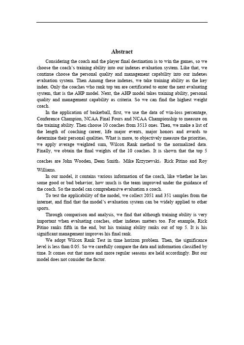
Abstract
Considering the coach and the player final destination is to win the games, so we choose the coach’s training ability into our indexes evaluation system. Like that, we continue choose the personal quality and management capability into our indexes evaluation system. Then Among these indexes, we take training ability as the key index. Only the coaches who rank top ten are certificated to enter the next evaluating system, that is the AHP model. Next, the AHP model takes training ability, personal quality and management capability as criteria. So we can find the highest weight coach. In the application of basketball, first, we use the data of win-loss percentage, Conference Champion, NCAA Final Fours and NCAA Championship to measure on the training ability. Then choose 10 coaches from 3513 ones. Then, we make a list of the length of coaching career, life major events, major honors and awards to determine their personal qualities. What is more, to objectively measure the priorities, we apply average weighted sum, Wilcox Rank method to the normalized data. Finally, we obtain the final weights of the 10 coaches. It is shown that the top 5 coaches are John Wooden, Dean Smith,Mike Krzyzewski,Rick Pitino and Roy Williams. In our model, it contains various information of the coach, like whether he has some good or bad behavior, how much is the team improved under the guidance of the coach. So the model can comprehensive evaluation a coach. To test the applicability of the model, we collect 2051 and 351 samples from the internet, and find that the model’s evaluation system can be widely applied to other sports. Through comparison and analysis, we find that although training ability is very important when evaluating coaches, other indexes matters too. For example, Rick Pitino ranks fifth in the end, but his training ability ranks out of top 5. It is his significant management improves his final rank. We adopt Wilcox Rank Test in time horizon problem. Then, the significance level is less than 0.05. So we carefully compare the data and information classified by time. It comes out that more and more regular seasons are held accordingly. But our model does not consider the factor.
2014年美国“数学大联盟杯赛”(中国赛区)初赛七年级(初一)详解

(七年级) 一、 选择题 1. B. No even number can be written as the product of two odd integers. Since 11 is the product of 1 and 11, Skip may have run 11 kilometers. A) 10 B) 11 C) 12 D) 14
27. D. As shown, only choice D is not a product of a divisor of 24 and a divisor of 35.
A) 1 × 1 B) 6 × 7 C) 8 × 7 D) 6 × 11 28. B. The sum of the dimensions is 40 ÷2 = 20. Its dimensions are 16 × 4, and its area is 64. A) 100 B) 64 C) 40 D) 24 29. A. Her average score for 6 tests was 82. So her total was 6 × 82 = 492. Adding 2 × 98, her total for 8 tests was 688. Her average score was 86. A) 86 B) 88 C) 90 D) 94 30. D. From 1 to 99 there are 9; in every 100 #s after there are 19. Include 1000. A) 162 B) 171 C) 180 D) 181 二、填空题 31. 8. 32. 2257. 33. 21. 34. 37. 35. 120. 36. 7410. 37. 2. 38. 81. 39. 32451. 40. 671.
2014年美国数学竞赛AMC8题目和答案解析

2.3.What is the value of ?4.Eight friends ate at a restaurant and agreed to share the bill equally. Because Judi forgot her money, each of her seven friends paid an extra $2.50 to cover her portion of the total bill. What was the total bill?5.Hammie is in the grade and weighs 106 pounds. His quadruplet sisters are tiny babies and weigh 5, 5, 6, and 8 pounds. Which is greater, the average (mean) weight of these five children or the median weight, and by how many pounds?6.The number in each box below is the product of the numbers in the two boxes that touch it in the row above. For example, . What is the missing number in the top row?7.Trey and his mom stopped at a railroad crossing to let a train pass. As the train began to pass, Trey counted 6 cars in the first 10 seconds. It took the train 2 minutes and 45 seconds to clear the crossing at a constant speed. Which of the following was the most likely number of cars in the train?8.A fair coin is tossed 3 times. What is the probability of at least two consecutive heads?9.The Incredible Hulk can double the distance he jumps with each succeeding jump. If his first jump is 1 meter, the second jump is 2 meters, the third jump is 4 meters, and so on, then on which jump will he first be able to jump more than 1 kilometer?10.What is the ratio of the least common multiple of 180 and 594 to the greatest common factor of 180 and 594?11. Ted's grandfather used his treadmill on 3 days this week. He went 2 miles each day. On Monday he joggedat a speed of 5 miles per hour. He walked at the rate of 3 miles per hour on Wednesday and at 4 miles perhour on Friday. If Grandfather had always walked at 4 miles per hour, he would have spent less time on the treadmill. How many minutes less?12. At the 2013 Winnebago County Fair a vendor is offering a "fair special" on sandals. If you buy one pairof sandals at the regular price of $50, you get a second pair at a 40% discount, and a third pair at half the regular price. Javier took advantage of the "fair special" to buy three pairs of sandals. What percentage of the $150 regular price did he save?13.When Clara totaled her scores, she inadvertently reversed the units digit and the tens digit of one score.By which of the following might her incorrect sum have differed from the correct one?14. Let the two digits be and .The correct score was . Clara misinterpreted it as . The difference between the two is which factors into . Therefore, since the difference is a multiple of 9, the only answer choice that is a multiple of 9 is .15. If , , and , what is the product of , , and ?16. A number of students from Fibonacci Middle School are taking part in a community service project. Theratio of -graders to -graders is , and the the ratio of -graders to -graders is . What is the smallest number of students that could be participating in the project?17. The sum of six consecutive positive integers is 2013. What is the largest of these six integers?18. Isabella uses one-foot cubical blocks to build a rectangular fort that is 12 feet long, 10 feet wide,and 5 feet high. The floor and the four walls are all one foot thick. How many blocks does the fort contain?--Arpanliku 16:22, 27 November 2013 (EST) Courtesy of Lord.of.AMC19. Bridget, Cassie, and Hannah are discussing the results of their last math test. Hannah shows Bridget andCassie her test, but Bridget and Cassie don't show theirs to anyone. Cassie says, 'I didn't get the lowest score in our class,' and Bridget adds, 'I didn't get the highest score.' What is the ranking of the three girls from highest to lowest?20. A rectangle is inscribed in a semicircle with longer side on the diameter. What is the area of thesemicircle?21.Samantha lives 2 blocks west and 1 block south of the southwest corner of City Park. Her school is 2 blockseast and 2 blocks north of the northeast corner of City Park. On school days she bikes on streets to the southwest corner of City Park, then takes a diagonal path through the park to the northeast corner, and then bikes on streets to school. If her route is as short as possible, how many different routes can she take?22.Toothpicks are used to make a grid that is 60 toothpicks long and 32 toothpicks wide. How many toothpicksare used altogether?23.Angle of is a right angle. The sides of are the diameters of semicircles as shown. The area of the semicircle on equals , and the arc of the semicircle on has length . What isthe radius of the semicircle on ?24. Squares , , and are equal in area. Points and are the midpoints of sidesand , respectively. What is the ratio of the area of the shaded pentagon to the sum of the areas of the three squares?25. A ball with diameter 4 inches starts at point A to roll along the track shown. The track is comprisedof 3 semicircular arcs whose radii are inches, inches, and inches, respectively. The ball always remains in contact with the track and does not slip. What is the distance the center of theball travels over the course from A to B?1.2.The 50% off price of half a pound of fish is $3, so the 100%, or the regular price, of a half pound of fish is $6. Consequently, if half a pound of fish costs $6, then a whole pound of fish is dollars.3.Notice that we can pair up every two numbers to make a sum of 1:Therefore, the answer is .4.Each of her seven friends paid to cover Judi's portion. Therefore, Judi's portion must be . Since Judi was supposed to pay of the total bill, the total bill must be .5.The median here is obviously less than the mean, so option (A) and (B) are out.Lining up the numbers (5, 5, 6, 8, 106), we see that the median weight is 6 pounds.The average weight of the five kids is .Therefore, the average weight is bigger, by pounds, making the answer .6.Solution 1: Working BackwardsLet the value in the empty box in the middle row be , and the value in the empty box in the top row be . is the answer we're looking for.We see that , making .It follows that , so .Solution 2: Jumping Back to the StartAnother way to do this problem is to realize what makes up the bottommost number. This method doesn't work quite as well for this problem, but in a larger tree, it might be faster. (In this case, Solution 1 would be faster since there's only two missing numbers.)Again, let the value in the empty box in the middle row be , and the value in the empty box in the top row be . is the answer we're looking for.We can write some equations:Now we can substitute into the first equation using the two others:7.If Trey saw , then he saw .2 minutes and 45 seconds can also be expressed as seconds.Trey's rate of seeing cars, , can be multiplied by on the top and bottom (and preserve the same rate):. It follows that the most likely number of cars is . Solution 2minutes and seconds is equal to .Since Trey probably counts around cars every seconds, there are groups of cars that Trey most likely counts. Since , the closest answer choice is .8.First, there are ways to flip the coins, in order.The ways to get two consecutive heads are HHT and THH.The way to get three consecutive heads is HHH.Therefore, the probability of flipping at least two consecutive heads is .9.This is a geometric sequence in which the common ratio is 2. To find the jump that would be over a 1000 meters, we note that .However, because the first term is and not , the solution to the problem is10. To find either the LCM or the GCF of two numbers, always prime factorize first.The prime factorization of .The prime factorization of .Then, find the greatest power of all the numbers there are; if one number is one but not the other, use it (this is ). Multiply all of these to get 5940.For the GCF of 180 and 594, use the least power of all of the numbers that are in both factorizations and multiply. = 18.Thus the answer = = .We start off with a similar approach as the original solution. From the prime factorizations, the GCF is .It is a well known fact that . So we have,.Dividing by yields .Therefore, .11.We use that fact that . Let d= distance, r= rate or speed, and t=time. In this case, let represent the time.On Monday, he was at a rate of . So, .For Wednesday, he walked at a rate of . Therefore, .On Friday, he walked at a rate of . So, .Adding up the hours yields + + = .We now find the amount of time Grandfather would have taken if he walked at per day. Set up the equation,.To find the amount of time saved, subtract the two amounts: - = . To convert this to minutes, we multiply by .Thus, the solution to this problem is12. First, find the amount of money one will pay for three sandals without the discount. We have.Then, find the amount of money using the discount: .Finding the percentage yields .To find the percent saved, we have13. Let the two digits be and .The correct score was . Clara misinterpreted it as . The difference between the two is which factors into . Therefore, since the difference is a multiple of 9, the only answer choice that is a multiple of 9 is .14. The probability that both show a green bean is . The probability that both show a red bean is . Therefore the probability is15.Therefore, .Therefore, .To most people, it would not be immediately evident that , so we can multiply 6's until we get the desired number:, so .Therefore the answer is .16. Solution 1: AlgebraWe multiply the first ratio by 8 on both sides, and the second ratio by 5 to get the same number for 8th graders, in order that we can put the two ratios together:Therefore, the ratio of 8th graders to 7th graders to 6th graders is . Since the ratio is in lowest terms, the smallest number of students participating in the project is .Solution 2: FakesolvingThe number of 8th graders has to be a multiple of 8 and 5, so assume it is 40 (the smallest possibility). Then there are 6th graders and 7th graders. The numbers of students is17. Solution 1The mean of these numbers is . Therefore the numbers are , so the answer isSolution 2Let the number be . Then our desired number is .Our integers are , so we have that.Solution 3Let the first term be . Our integers are . We have,18. Solution 1There are cubes on the base of the box. Then, for each of the 4 layers above the bottom (as since each cube is 1 foot by 1 foot by 1 foot and the box is 5 feet tall, there are 4 feet left), there arecubes. Hence, the answer is .Solution 2We can just calculate the volume of the prism that was cut out of the original box. Each interior side of the fort will be feet shorter than each side of the outside. Since the floor is foot, the height will be feet. So the volume of the interior box is .The volume of the original box is . Therefore, the number of blocks contained in thefort is .19. If Hannah did better than Cassie, there would be no way she could know for sure that she didn't get thelowest score in the class. Therefore, Hannah did worse than Cassie. Similarly, if Hannah did worse than Bridget, there is no way Bridget could have known that she didn't get the highest in the class. Therefore, Hannah didbetter than Bridget, so our order is .20.A semicircle has symmetry, so the center is exactly at the midpoint of the 2 side on the rectangle, making the radius, by the Pythagorean Theorem, . The area is .21.The number of ways to get from Samantha's house to City Park is , and the number of ways to get from City Park to school is . Since there's one way to go through City Park (just walking straight through), the number of different ways to go from Samantha's house to City Park to school .22.There are vertical columns with a length of toothpicks, and there are horizontal rows with a length of toothpicks. An effective way to verify this is to try a small case, i.e. a grid of toothpicks. Thus, our answer is .23. Solution 1If the semicircle on AB were a full circle, the area would be 16pi. Therefore the diameter of the first circle is 8. The arc of the largest semicircle would normally have a complete diameter of 17. The Pythagorean theoremsays that the other side has length 15, so the radius is .Solution 2We go as in Solution 1, finding the diameter of the circle on AC and AB. Then, an extended version of the theorem says that the sum of the semicircles on the left is equal to the biggest one, so the area of the largestis , and the middle one is , so the radius is .24.First let (where is the side length of the squares) for simplicity. We can extend until it hitsthe extension of . Call this point . The area of triangle then is The area of rectangle is . Thus, our desired area is . Now, the ratio of the shaded area to the combinedarea of the three squares is .Solution 2Let the side length of each square be .Let the intersection of and be .Since , . Since and are vertical angles, they are congruent. We also have by definition.So we have by congruence. Therefore, .Since and are midpoints of sides, . This combined with yields.The area of trapezoid is .The area of triangle is .So the area of the pentagon is .The area of the squares is .Therefore, .Solution 3Let the intersection of and be .Now we have and .Because both triangles has a side on congruent squares therefore .Because and are vertical angles .Also both and are right angles so .Therefore by AAS(Angle, Angle, Side) .Then translating/rotating the shaded into the position ofSo the shaded area now completely covers the squareSet the area of a square asTherefore, .25. Solution 1The radius of the ball is 2 inches. If you think about the ball rolling or draw a path for the ball (see figure below), you see that in A and C it loses inches, and it gains inches on B.So, the departure from the length of the track means that the answer is . Solution 2The total length of all of the arcs is . Since we want the path from the center, the actual distance will be shorter. Therefore, the only answer choice less than is . Thissolution may be invalid because the actual distance can be longer if the path the center travels is on the outside of the curve, as it is in the middle bump.。
2014年美国“数学大联盟杯赛”(中国赛区)初赛八、九年级试卷
34. The sum of 5 different prime numbers is 200. Each of the 5 prime numbers is less than 100. Four of the 5 prime numbers have the same units digit. What is the median of the 5 prime numbers? Answer:______. 35. The sum of the digits of 2014 is 2 + 0 + 1 + 4 = 7. For how many numbers between 1 and 10000 is the sum of the digits of each number 29? Answer:______. 36. Tom has 6 cards with number 1 on each card, 3 cards with number 2 on each card, 5 cards with number 3 on each card, 1 card with number 5 it, 3 cards with number 7 on each card, and 2 cards with number 9 on each card. So Tom has 20 cards in total. He uses all these 20 cards to form 12 different prime numbers. Each primer number is either a number on a card, or a number from concatenating the two numbers on two cards. (Card with number 9 can’t be used as number 6, and vice versa.) The product of all the 12 prime numbers is ab207381348cd . What is abcd ? Answer:______. 37. Ten people stand to form a line, p1, p2 , p3 , p4 , p5 , p6 , p7 , p8 , p9 , p10 , with p1 the leftmost person. Some of them are truth-tellers who always speak the truth. And the rest are all liars who always lie. p1 stated that there are 3 liars to my right. p2 stated that there is one liar to my left. p3 stated that there are 4 liars to my right. p4 stated that there is one liar to my left. p5 stated that there are 5 liars to my right. p6 stated that there are 9 liars in total. p8 stated that there are 6 liars to my left. p7 stated that there are 2 liars to my right. p10 stated that there are 3 liars to my left. p9 stated that there are 5 liars to my left. How many truth-tellers are there? Answer:______. 38. Sn denotes the sum of all the digits of integer n. For example, S123 = 1 + 2 + 3 = 6. Two different integers m and n form a pair, <m, n>, where m < 100, n < 100, m < n, and m + Sm = n + Sn. How many such pairs, <m, n>, exist? Answer:______. 39. Place numbers 14, 27, 36, 57, 178, 467, 590, and 2345 on the eight vertexes of an octagon such that any two numbers on two adjacent vertexes share some same digit(s). What is the sum of the two numbers adjacent to 57? Answer:______. 40. If a 4-digit number, which is a perfect square, can be written as aabb cc , it is called a "good" perfect square number. How many “good” perfect square numbers are there? Answer:______.
98804462_4_作业2014两道题

《数学建模引论》作业题(要求第12周以前完成)[注] 本作业中的两个问题都是美国中学生数学建模竞赛(HiMCM)过去的竞赛题。
请特别注意:数学建模题通常没有标准答案,大家可以自由发挥想象力、洞察力;但请务必清晰、完整地列出你的模型假设,然后分析你所考虑的相关因素之间的关系,从而建立数学模型,并求解模型和解释你的结论。
也就是说,你的作业应该完整体现数学建模的全过程。
(要求每人独立完成,可以通过网络学堂提交电子版;也可以第12周课上提交手写版)。
1、HiMCM-2007 Problem B: Car Rentals (租车问题)Some people rent a car when they are going on a long trip. They are convinced they save money. Even if they do not save money, they feel that the knowledge that "if the car breaks down on the trip, the problem is the rental company's" makes the rental worth it. Analyze this situation and determine under what conditions renting a car is a more appropriate option. Determine mileage limits on one's own car and a break-even value of "ease of mind" for the driver and her family.(参考译文:有些人当他们将要做一个长途旅行的时候,他们会租一辆汽车。
他们通常觉得这样会省钱。
2014美国数学建模竞赛 MCM A题 参考答案 元胞自动机
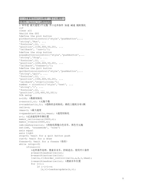
clfclear all%build the GUI%define the plot buttonplotbutton=uicontrol('style','pushbutton',...'string','Run', ...'fontsize',12, ...'position',[100,400,50,20], ...'callback', 'run=1;');%define the stop buttonerasebutton=uicontrol('style','pushbutton',...'string','Stop', ...'fontsize',12, ...'position',[200,400,50,20], ...'callback','freeze=1;');%define the Quit buttonquitbutton=uicontrol('style','pushbutton',...'string','Quit', ...'fontsize',12, ...'position',[300,400,50,20], ...'callback','stop=1;close;');number = uicontrol('style','text', ...'string','1', ...'fontsize',12, ...'position',[20,400,50,20]);%CA setupn=100;%数据初始化z=zeros(1,n);%元胞个数z=roadstart(z,5);%道路状态初始化,路段上随机分布5辆cells=z;vmax=3;%最大速度v=speedstart(cells,vmax);%速度初始化x=1;%记录速度和车辆位置memor_cells=zeros(3600,n);memor_v=zeros(3600,n);imh=imshow(cells);%初始化图像白色有车,黑色空元胞set(imh, 'erasemode', 'none')axis equalaxis tightstop=0; %wait for a quit button pushrun=0; %wait for a drawfreeze=0; %wait for a freeze(冻结)while (stop==0)if(run==1)%边界条件处理,搜素首末车,控制进出,使用开口条件a=searchleadcar(cells);b=searchlastcar(cells);[cells,v]=border_control(cells,a,b,v,vmax); i=searchleadcar(cells);%搜索首车位置for j=1:iif i-j+1==n[z,v]=leadcarupdate(z,v);continue;else%======================================加速、减速、随机慢化 if cells(i-j+1)==0;%判断当前位置是否非空continue;else v(i-j+1)=min(v(i-j+1)+1,vmax);%加速%=================================减速k=searchfrontcar((i-j+1),cells);%搜素前方首个非空元胞位置if k==0;%确定于前车之间的元胞数d=n-(i-j+1);else d=k-(i-j+1)-1;endv(i-j+1)=min(v(i-j+1),d);%==============================%减速%随机慢化v(i-j+1)=randslow(v(i-j+1));new_v=v(i-j+1);%======================================加速、减速、随机慢化%更新车辆位置z(i-j+1)=0;z(i-j+1+new_v)=1;%更新速度v(i-j+1)=0;v(i-j+1+new_v)=new_v;endendendcells=z;memor_cells(x,:)=cells;%记录速度和车辆位置memor_v(x,:)=v;x=x+1;set(imh,'cdata',cells)%更新图像%update the step number diaplaypause(0.2);stepnumber = 1 + str2num(get(number,'string'));set(number,'string',num2str(stepnumber))endif (freeze==1)run = 0;freeze = 0;enddrawnowend///////////////////////////////////////////////////////////////////////Function[new_matrix_cells,new_v]=border_control(matrix_cells,a,b,v,vmax) %边界条件,开口边界,控制车辆出入%出口边界,若头车在道路边界,则以一定该路0.9离去n=length(matrix_cells);if a==nrand('state',sum(100*clock)*rand(1));%¶¨ÒåËæ»úÖÖ×Óp_1=rand(1);%产生随机概率if p_1<=1 %如果随机概率小于0.9,则车辆离开路段,否则不离口matrix_cells(n)=0;v(n)=0;endend%入口边界,泊松分布到达,1s内平均到达车辆数为q,t为1sif b>vmaxt=1;q=0.25;x=1;p=(q*t)^x*exp(-q*t)/prod(x);%1s内有1辆车到达的概率rand('state',sum(100*clock)*rand(1));p_2=rand(1);if p_2<=pm=min(b-vmax,vmax);matrix_cells(m)=1;v(m)=m;endendnew_matrix_cells=matrix_cells;new_v=v;///////////////////////////////////////////////////////////////////////function [new_matrix_cells,new_v]=leadcarupdate(matrix_cells,v)%第一辆车更新规则n=length(matrix_cells);if v(n)~=0matrix_cells(n)=0;v(n)=0;endnew_matrix_cells=matrix_cells;new_v=v;///////////////////////////////////////////////////////////////////////function [new_v]=randslow(v)p=0.3;%慢化概率rand('state',sum(100*clock)*rand(1));%¶¨ÒåËæ»úÖÖ×Óp_rand=rand;%产生随机概率if p_rand<=pv=max(v-1,0);endnew_v=v;///////////////////////////////////////////////////////////////////////function [matrix_cells_start]=roadstart(matrix_cells,n)%道路上的车辆初始化状态,元胞矩阵随机为0或1,matrix_cells初始矩阵,n初始车辆数k=length(matrix_cells);z=round(k*rand(1,n));for i=1:nj=z(i);if j==0matrix_cells(j)=0;elsematrix_cells(j)=1;endendmatrix_cells_start=matrix_cells;///////////////////////////////////////////////////////////////////////function[location_frontcar]=searchfrontcar(current_location,matrix_cells)i=length(matrix_cells);if current_location==ilocation_frontcar=0;elsefor j=current_location+1:iif matrix_cells(j)~=0location_frontcar=j;break;elselocation_frontcar=0;endendend///////////////////////////////////////////////////////////////////////function [location_lastcar]=searchlastcar(matrix_cells)%搜索尾车位置for i=1:length(matrix_cells)if matrix_cells(i)~=0location_lastcar=i;break;else %如果路上无车,则空元胞数设定为道路长度location_lastcar=length(matrix_cells);endend///////////////////////////////////////////////////////////////////////function [location_leadcar]=searchleadcar(matrix_cells)i=length(matrix_cells);for j=1:iif matrix_cells(i-j+1)~=0location_leadcar=i-j+1;break;elselocation_leadcar=0;endend///////////////////////////////////////////////////////////////////////function [v_matixcells]=speedstart(matrix_cells,vmax)%道路初始状态车辆速度初始化v_matixcells=zeros(1,length(matrix_cells));for i=1:length(matrix_cells)if matrix_cells(i)~=0v_matixcells(i)=round(vmax*rand(1));endend。
2014年美国数学建模比赛试题、翻译和分析(终稿)

ROBLEM A: The Keep-Right-Except-To-Pass Rule问题A:除非超车否则靠右行驶的交通规则In countries where driving automobiles on the right is the rule (that is, USA, China and most other countries except for Great Britain, Australia, and some former British colonies), multi-lane freeways often employ a rule that requires drivers to drive in the right-most lane unless they are passing another vehicle, in which case they move one lane to the left, pass, and return to their former travel lane.在一些汽车靠右行驶的国家(比如美国,中国等等),多车道的高速公路常常遵循以下原则:司机必须在最右侧驾驶,除非他们正在超车,超车时必须先移到左侧车道在超车后再返回。
Build and analyze a mathematical model to analyze the performance of this rule in light and heavy traffic. You may wish to examine tradeoffs between traffic flow and safety, the role of under- or over-posted speed limits (that is, speed limits that are too low or too high), and/or other factors that may not be explicitly called out in this problem statement. Is this rule effective in promoting better traffic flow? If not, suggest and analyze alternatives (to include possibly no rule of this kind at all) that might promote greater traffic flow, safety, and/or other factors that you deem important.建立数学模型来分析这条规则在低负荷和高负荷状态下的交通路况的表现。
2014 年美国大学生数学建模竞赛 MCM

2014 年美国大学生数学建模竞赛MCM、ICM 试题2014 MCM A: The Keep-Right-Except-To-Pass RuleIn countries where driving automobiles on the right is the rule (that is, USA, China and most other countries except for Great Britain, Australia, and some former British colonies), multi-lane freeways often employ a rule that requires drivers to drive in the right-most lane unless they are passing another vehicle, in which case they move one lane to the left, pass, and return to their former travel lane.Build and analyze a mathematical model to analyze the performance of this rule in light and heavy traffic. You may wish to examine tradeoffs between traffic flow and safety, the role of under- or over-posted speed limits (that is, speed limits that are too low or too high), and/or other factors that may not be explicitly called out in this problem statement. Is this rule effective in promoting better traffic flow? If not, suggest and analyze alternatives (to include possibly no rule of this kind at all) that might promote greater traffic flow, safety, and/or other factors that you deem important.In countries where driving automobiles on the left is the norm, argue whether or not your solution can be carried over with a simple change of orientation, or would additional requirements be needed.Lastly, the rule as stated above relies upon human judgment for compliance. If vehicle transportation on the same roadway was fully under the control of an intelligent system –either part of the road network or imbedded in the design of all vehicles using the roadway – to what extent would this change the results of your earlier analysis?2014 MCM B: College Coaching LegendsSports Illustrated, a magazine for sports enthusiasts, is looking for the “best all time college coach” male or fem ale for the previous century. Build a mathematical model to choose the best college coach or coaches (past or present) from among either male or female coaches in such sports as college hockey or field hockey, football, baseball or softball, basketball, or soccer. Does it make a difference which time line horizon that you use in your analysis, i.e., does coaching in 1913 differ from coaching in 2013? Clearly articulate your metrics for assessment. Discuss how your model can be applied in general across both genders and all possible sports. Present your model’s top 5 coaches in each of 3 different sports.In addition to the MCM format and requirements, prepare a 1-2 page article for Sports Illustrated that explains your results and includes a non-technical explanation of your mathematical model that sports fans will understand.。
2014年美国数学建模比赛B题(最佳教练)

B
Summary
2014 Mathematical Contest in Modeling (MCM) Summary Sheet
This paper mainly sets a model of selecting five “best all time college coach” in basketball, football and hockey respectively. The model is separated to six sub-problems and its solution in our paper:1)Selecting the best coach in one NCAA basketball season; 2)Screening the college coach at top-20 to top-30 in the past 100 years; 3)Further analysis to these selected coaches, and ranking the top-5; 4)Applying this model to football and hockey; 5)Gender impact analysis and time impact analysis; 6)Analyzing the reasons that some famous coach selected by some magazines and media are not on our ranking list. For sub-problem1:Identify four indicators, and confirm the weight of each indicator by Analytic Hierarchy Process, then transformer the indicator data into scores and add these scores multiplied by the weight of itself to get the final scores. The best coach in one season is the one with highest score. For sub-problem2: Use the method above to score for all of the coaches in the past 100 years , then select the top-20.For purpose of reducing the influence of subjective factors, we use Principal Component Analysis to get another ranking list, also, we select the top-20.And union these two top-20. For sub-problem3:Surveying these coaches in the union to learn how many NBA players they've respectively brought up. And regarding this as an indicator, then dividing all indicators into Experience,Leading ability and Ability of player cultivation three aspects, and using Multilevel Hierarchical Analysis to weight them. Next, score for each person by the Fuzzy Criterion of Composite and rank according to the scores. With the purpose of reducing the influence of subjective factors, using Grey Correlation Analysis to calculate the grey correlation degree between “perfect coach” and these coaches. After that, using t-test to judge whether the two results with significant differences. The conclusion obtained: There are no significant difference. Namely, this method is generality. For sub-problem4:Fine-tuning part of indicators and weights, then apply this model in football and hockey. For sub-problem5:As One-way Analysis of Variance used, and the conclusion obtained: gender doesn’t affect the overall score or the ranking of coaches, but female coach has unique advantages in women's basketball league. And the time has no significant effect on the comprehensive score ,but the most excellent coach were in the 70s. Combined with the history of NCAA development, we think that it is necessary to improve the weight of the indicator---champions that gotten recently, making this model better. .For sub-problem6: Comparing the data of their career with our standards to find the reasons.
2014年美国大学生数学建模大赛赛题
2014 MCM ProblemsPROBLEM A: The Keep-Right-Except-To-Pass RuleIn countries where driving automobiles on the right is the rule (that is, USA, China and most other countries except for Great Britain, Australia, and some former British colonies), multi-lane freeways often employ a rule that requires drivers to drive in the right-most lane unless they arepassing another vehicle, in which case they move one lane to the left,pass, and return to their former travel lane.Build and analyze a mathematical model to analyze the performance of this rule in light and heavy traffic. You may wish to examine tradeoffs between traffic flow and safety, the role of under- or over-posted speed limits (that is, speed limits that are too low or too high), and/or other factors that may not be explicitly called out in this problem statement. Is this rule effective in promoting better traffic flow? If not, suggest and analyze alternatives (to include possibly no rule of this kind at all) that might promote greater traffic flow, safety, and/or other factors that you deem important.In countries where driving automobiles on the left is the norm, argue whether or not your solution can be carried over with a simple change of orientation, or would additional requirements be needed.Lastly, the rule as stated above relies upon human judgment for compliance. If vehicle transportation on the same roadway was fully under the control of an intelligent system – either part of the road network or imbedded in the design of all vehicles using the roadway – to what extent would this change the results of your earlier analysis?PROBLEM B: College Coaching LegendsSports Illustrated, a magazine for sports enthusiasts, is looking for the “best all time college coach” male or female for the previous century. Build a mathematical model to choose the best college coach or coaches (past or present) from among either male or female coaches in such sports as college hockey or field hockey, football, baseball or softball, basketball, or soccer. Does it make a difference which time line horizon that you use in your analysis, i.e., does coaching in 1913 differ from coaching in 2013? Clearly articulate yourmetrics for assessment. Discuss how your model can be applied in general across both gen ders and all possible sports. Present your model’s top 5 coaches in each of 3 different sports.In addition to the MCM format and requirements, prepare a 1-2 page article for Sports Illustrated that explains your results and includes a non-technical explanation of your mathematical model that sports fans will understand.。
- 1、下载文档前请自行甄别文档内容的完整性,平台不提供额外的编辑、内容补充、找答案等附加服务。
- 2、"仅部分预览"的文档,不可在线预览部分如存在完整性等问题,可反馈申请退款(可完整预览的文档不适用该条件!)。
- 3、如文档侵犯您的权益,请联系客服反馈,我们会尽快为您处理(人工客服工作时间:9:00-18:30)。
HIMCM 2014美国中学生数学建模竞赛试题Problem A: Unloading Commuter TrainsTrains arrive often at a central Station, the nexus for many commuter trains from suburbs of larger cities on a “commuter” line. Most trains are long (perhaps 10 or more cars long). The distance a passenger has to walk to exit the train area is quite long. Each train car has only two exits, one near each end so that the cars can carry as many people as possible. Each train car has a center aisle and there are two seats on one side and three seats on the other for each row of seats.To exit a typical station of interest, passengers must exit the car, and then make their way to a stairway to get to the next level to exit the station. Usually these trains are crowded so there is a “fan” of passengers from the train trying to get up the stairway. The stairway could accommodate two columns of people exiting to the top of the stairs.Most commuter train platforms have two tracks adjacent to the platform. In the worst case, if two fully occupied trains arrived at the same time, it might take a long time for all the passengers to get up to the main level of the station.Build a mathematical model to estimate the amount of time for a passenger to reach the street level of the station to exit the complex. Assume there are n cars to a train, each car has length d. The length of the platform is p, and the number of stairs in each staircase is q. Use your model to specifically optimize (minimize) the time traveled to reach street level to exit a station for the following:问题一:通勤列车的负载问题在中央车站,经常有许多的联系从大城市到郊区的通勤列车“通勤”线到达。
大多数火车很长(也许10个或更多的汽车长)。
乘客走到出口的距离也很长,有整个火车区域。
每个火车车厢只有两个出口,一个靠近终端, 因此可以携带尽可能多的人。
每个火车车厢有一个中心过道和过道两边的座椅,一边每排有两个座椅,另一边每排有三个座椅。
走出这样一个典型车站,乘客必须先出火车车厢,然后走入楼梯再到下一个级别的出站口。
通常情况下这些列车都非常拥挤,有大量的火车上的乘客试图挤向楼梯,而楼梯可以容纳两列人退出。
大多数通勤列车站台有两个相邻的轨道平台。
在最坏的情况下,如果两个满载的列车同时到达,所有的乘客可能需要很长时间才能到达主站台。
建立一个数学模型来估计旅客退出这种复杂的状况到达出站口路上的时间。
假设一列火车有n个汽车那么长,每个汽车的长度为d。
站台的长度是p,每个楼梯间的楼梯数量是q。
使用您的模型具体来优化(减少)前往主站台的时间,有如下要求:Requirement 1. One fully occupied train's passengers to exit the train, and ascend the stairs to reach the street access level of the station.要求1.一个满载乘客的火车,所有乘客都要出火车。
所有乘客都要出楼梯抵达出主站台的路上。
Requirement 2. Two fully occupied trains' passengers (all passengers exit onto a common platform) to exit the trains, and ascend the stairs to reach the street access levelof the station.要求2.两个满载列车的乘客都要出车厢(所有乘客出到一个公用站台), 所有乘客都要出楼梯抵达出主站台的路上。
Requirement 3. If you could redesign the location of the stairways along the platform, where should these stairways be placed to minimize the time for one or two trains' passengers to exit the station?要求3.如果你能重新设计楼梯沿着站台的位置,那么这些楼梯应放置在哪,以缩短一列或两列火车的乘客出站所用的时间?Requirement 4. How does the time to street level vary with the number s of stairways that one builds?要求4.乘客到达出主站台的路上所用的时间跟构建楼梯的台阶数有怎样的关系?Requirement 5. How does the time vary if the stairways can accommodate k people, k an integer greater than one?要求5.如果楼梯可以容纳K个人,那么时间会如何变化?(k是大于1的整数)In addition to the HiMCM format, prepare a short non-technical article to the director of transportation explaining why they should adopt your model to improve exiting a station. 除了要遵循HiMCM规范,准备一个简短的非技术物品向运输主管解释为什么他们应该采取你的模型来提高出站效率。
Problem B: The Next Plague?In 2014, the world saw the infectious Ebola virus spreading in western Africa. Throughout human history, epidemics have come and gone with some infecting and/or killing thousands and lasting for years and others taking less of a human toll. Some believe these events are just nature’s way of controlling the growth of a species while others think they could be a conspiracy or deliberate act to cause harm. This problem will most likely come down to how to expend (or not expend) scarce resources (doctors, containment facilities, money, research, serums, etc…) to deal with a crisis.问题二:下一场瘟疫?在2014年,世界看到了感染埃博拉病毒在西非蔓延。
纵观人类历史,流行病来了又走,有些感染带到来然后杀死成千上万的人并且持续数百年,另外一些流行病导致少量的人员伤亡的。
一些人认为,这些事件只是大自然控制物种的生长方式,而其他人则认为,这可能是一个阴谋,或者是故意行为造成伤害。
这个问题很可能会归咎到如何花费(或不花费)稀缺资源(医生,防护设施,资金,科研,精华素等),以应对危机。
Section A:A routine humanitarian mission on an island in Indonesia reported a small village where almost half of its 300 inhabitants are showing similar symptoms. In the past week, 15 of the “infected” have died. This village is known to trade with nearby villages and other islands. Your modeling team works for a major center of disease control in the capital of your country (or if you prefer, for the International World Health Organization).A部分:一个常见的人道主义报道:在印度尼西亚的一个岛上的一个小村庄,那里的300名居民中几乎有一半都出现了类似的症状。