Robust Time-Delay Based Angle of Arrival Estimation

合集下载

引力波观测原文PhysRevLett.116.061102

Observation of Gravitational Waves from a Binary Black Hole MergerB.P.Abbott et al.*(LIGO Scientific Collaboration and Virgo Collaboration)(Received21January2016;published11February2016)On September14,2015at09:50:45UTC the two detectors of the Laser Interferometer Gravitational-Wave Observatory simultaneously observed a transient gravitational-wave signal.The signal sweeps upwards in frequency from35to250Hz with a peak gravitational-wave strain of1.0×10−21.It matches the waveform predicted by general relativity for the inspiral and merger of a pair of black holes and the ringdown of the resulting single black hole.The signal was observed with a matched-filter signal-to-noise ratio of24and a false alarm rate estimated to be less than1event per203000years,equivalent to a significance greaterthan5.1σ.The source lies at a luminosity distance of410þ160−180Mpc corresponding to a redshift z¼0.09þ0.03−0.04.In the source frame,the initial black hole masses are36þ5−4M⊙and29þ4−4M⊙,and the final black hole mass is62þ4−4M⊙,with3.0þ0.5−0.5M⊙c2radiated in gravitational waves.All uncertainties define90%credible intervals.These observations demonstrate the existence of binary stellar-mass black hole systems.This is the first direct detection of gravitational waves and the first observation of a binary black hole merger.DOI:10.1103/PhysRevLett.116.061102I.INTRODUCTIONIn1916,the year after the final formulation of the field equations of general relativity,Albert Einstein predicted the existence of gravitational waves.He found that the linearized weak-field equations had wave solutions: transverse waves of spatial strain that travel at the speed of light,generated by time variations of the mass quadrupole moment of the source[1,2].Einstein understood that gravitational-wave amplitudes would be remarkably small;moreover,until the Chapel Hill conference in 1957there was significant debate about the physical reality of gravitational waves[3].Also in1916,Schwarzschild published a solution for the field equations[4]that was later understood to describe a black hole[5,6],and in1963Kerr generalized the solution to rotating black holes[7].Starting in the1970s theoretical work led to the understanding of black hole quasinormal modes[8–10],and in the1990s higher-order post-Newtonian calculations[11]preceded extensive analytical studies of relativistic two-body dynamics[12,13].These advances,together with numerical relativity breakthroughs in the past decade[14–16],have enabled modeling of binary black hole mergers and accurate predictions of their gravitational waveforms.While numerous black hole candidates have now been identified through electromag-netic observations[17–19],black hole mergers have not previously been observed.The discovery of the binary pulsar system PSR B1913þ16 by Hulse and Taylor[20]and subsequent observations of its energy loss by Taylor and Weisberg[21]demonstrated the existence of gravitational waves.This discovery, along with emerging astrophysical understanding[22], led to the recognition that direct observations of the amplitude and phase of gravitational waves would enable studies of additional relativistic systems and provide new tests of general relativity,especially in the dynamic strong-field regime.Experiments to detect gravitational waves began with Weber and his resonant mass detectors in the1960s[23], followed by an international network of cryogenic reso-nant detectors[24].Interferometric detectors were first suggested in the early1960s[25]and the1970s[26].A study of the noise and performance of such detectors[27], and further concepts to improve them[28],led to proposals for long-baseline broadband laser interferome-ters with the potential for significantly increased sensi-tivity[29–32].By the early2000s,a set of initial detectors was completed,including TAMA300in Japan,GEO600 in Germany,the Laser Interferometer Gravitational-Wave Observatory(LIGO)in the United States,and Virgo in binations of these detectors made joint obser-vations from2002through2011,setting upper limits on a variety of gravitational-wave sources while evolving into a global network.In2015,Advanced LIGO became the first of a significantly more sensitive network of advanced detectors to begin observations[33–36].A century after the fundamental predictions of Einstein and Schwarzschild,we report the first direct detection of gravitational waves and the first direct observation of a binary black hole system merging to form a single black hole.Our observations provide unique access to the*Full author list given at the end of the article.Published by the American Physical Society under the terms of the Creative Commons Attribution3.0License.Further distri-bution of this work must maintain attribution to the author(s)and the published article’s title,journal citation,and DOI.properties of space-time in the strong-field,high-velocity regime and confirm predictions of general relativity for the nonlinear dynamics of highly disturbed black holes.II.OBSERVATIONOn September14,2015at09:50:45UTC,the LIGO Hanford,W A,and Livingston,LA,observatories detected the coincident signal GW150914shown in Fig.1.The initial detection was made by low-latency searches for generic gravitational-wave transients[41]and was reported within three minutes of data acquisition[43].Subsequently, matched-filter analyses that use relativistic models of com-pact binary waveforms[44]recovered GW150914as the most significant event from each detector for the observa-tions reported here.Occurring within the10-msintersite FIG.1.The gravitational-wave event GW150914observed by the LIGO Hanford(H1,left column panels)and Livingston(L1,rightcolumn panels)detectors.Times are shown relative to September14,2015at09:50:45UTC.For visualization,all time series are filtered with a35–350Hz bandpass filter to suppress large fluctuations outside the detectors’most sensitive frequency band,and band-reject filters to remove the strong instrumental spectral lines seen in the Fig.3spectra.Top row,left:H1strain.Top row,right:L1strain.GW150914arrived first at L1and6.9þ0.5−0.4ms later at H1;for a visual comparison,the H1data are also shown,shifted in time by this amount and inverted(to account for the detectors’relative orientations).Second row:Gravitational-wave strain projected onto each detector in the35–350Hz band.Solid lines show a numerical relativity waveform for a system with parameters consistent with those recovered from GW150914[37,38]confirmed to99.9%by an independent calculation based on[15].Shaded areas show90%credible regions for two independent waveform reconstructions.One(dark gray)models the signal using binary black hole template waveforms [39].The other(light gray)does not use an astrophysical model,but instead calculates the strain signal as a linear combination of sine-Gaussian wavelets[40,41].These reconstructions have a94%overlap,as shown in[39].Third row:Residuals after subtracting the filtered numerical relativity waveform from the filtered detector time series.Bottom row:A time-frequency representation[42]of the strain data,showing the signal frequency increasing over time.propagation time,the events have a combined signal-to-noise ratio(SNR)of24[45].Only the LIGO detectors were observing at the time of GW150914.The Virgo detector was being upgraded, and GEO600,though not sufficiently sensitive to detect this event,was operating but not in observational mode.With only two detectors the source position is primarily determined by the relative arrival time and localized to an area of approximately600deg2(90% credible region)[39,46].The basic features of GW150914point to it being produced by the coalescence of two black holes—i.e., their orbital inspiral and merger,and subsequent final black hole ringdown.Over0.2s,the signal increases in frequency and amplitude in about8cycles from35to150Hz,where the amplitude reaches a maximum.The most plausible explanation for this evolution is the inspiral of two orbiting masses,m1and m2,due to gravitational-wave emission.At the lower frequencies,such evolution is characterized by the chirp mass[11]M¼ðm1m2Þ3=5121=5¼c3G596π−8=3f−11=3_f3=5;where f and_f are the observed frequency and its time derivative and G and c are the gravitational constant and speed of light.Estimating f and_f from the data in Fig.1, we obtain a chirp mass of M≃30M⊙,implying that the total mass M¼m1þm2is≳70M⊙in the detector frame. This bounds the sum of the Schwarzschild radii of thebinary components to2GM=c2≳210km.To reach an orbital frequency of75Hz(half the gravitational-wave frequency)the objects must have been very close and very compact;equal Newtonian point masses orbiting at this frequency would be only≃350km apart.A pair of neutron stars,while compact,would not have the required mass,while a black hole neutron star binary with the deduced chirp mass would have a very large total mass, and would thus merge at much lower frequency.This leaves black holes as the only known objects compact enough to reach an orbital frequency of75Hz without contact.Furthermore,the decay of the waveform after it peaks is consistent with the damped oscillations of a black hole relaxing to a final stationary Kerr configuration. Below,we present a general-relativistic analysis of GW150914;Fig.2shows the calculated waveform using the resulting source parameters.III.DETECTORSGravitational-wave astronomy exploits multiple,widely separated detectors to distinguish gravitational waves from local instrumental and environmental noise,to provide source sky localization,and to measure wave polarizations. The LIGO sites each operate a single Advanced LIGO detector[33],a modified Michelson interferometer(see Fig.3)that measures gravitational-wave strain as a differ-ence in length of its orthogonal arms.Each arm is formed by two mirrors,acting as test masses,separated by L x¼L y¼L¼4km.A passing gravitational wave effec-tively alters the arm lengths such that the measured difference isΔLðtÞ¼δL x−δL y¼hðtÞL,where h is the gravitational-wave strain amplitude projected onto the detector.This differential length variation alters the phase difference between the two light fields returning to the beam splitter,transmitting an optical signal proportional to the gravitational-wave strain to the output photodetector. To achieve sufficient sensitivity to measure gravitational waves,the detectors include several enhancements to the basic Michelson interferometer.First,each arm contains a resonant optical cavity,formed by its two test mass mirrors, that multiplies the effect of a gravitational wave on the light phase by a factor of300[48].Second,a partially trans-missive power-recycling mirror at the input provides addi-tional resonant buildup of the laser light in the interferometer as a whole[49,50]:20W of laser input is increased to700W incident on the beam splitter,which is further increased to 100kW circulating in each arm cavity.Third,a partially transmissive signal-recycling mirror at the outputoptimizes FIG. 2.Top:Estimated gravitational-wave strain amplitude from GW150914projected onto H1.This shows the full bandwidth of the waveforms,without the filtering used for Fig.1. The inset images show numerical relativity models of the black hole horizons as the black holes coalesce.Bottom:The Keplerian effective black hole separation in units of Schwarzschild radii (R S¼2GM=c2)and the effective relative velocity given by the post-Newtonian parameter v=c¼ðGMπf=c3Þ1=3,where f is the gravitational-wave frequency calculated with numerical relativity and M is the total mass(value from Table I).the gravitational-wave signal extraction by broadening the bandwidth of the arm cavities [51,52].The interferometer is illuminated with a 1064-nm wavelength Nd:Y AG laser,stabilized in amplitude,frequency,and beam geometry [53,54].The gravitational-wave signal is extracted at the output port using a homodyne readout [55].These interferometry techniques are designed to maxi-mize the conversion of strain to optical signal,thereby minimizing the impact of photon shot noise (the principal noise at high frequencies).High strain sensitivity also requires that the test masses have low displacement noise,which is achieved by isolating them from seismic noise (low frequencies)and designing them to have low thermal noise (intermediate frequencies).Each test mass is suspended as the final stage of a quadruple-pendulum system [56],supported by an active seismic isolation platform [57].These systems collectively provide more than 10orders of magnitude of isolation from ground motion for frequen-cies above 10Hz.Thermal noise is minimized by using low-mechanical-loss materials in the test masses and their suspensions:the test masses are 40-kg fused silica substrates with low-loss dielectric optical coatings [58,59],and are suspended with fused silica fibers from the stage above [60].To minimize additional noise sources,all components other than the laser source are mounted on vibration isolation stages in ultrahigh vacuum.To reduce optical phase fluctuations caused by Rayleigh scattering,the pressure in the 1.2-m diameter tubes containing the arm-cavity beams is maintained below 1μPa.Servo controls are used to hold the arm cavities on resonance [61]and maintain proper alignment of the optical components [62].The detector output is calibrated in strain by measuring its response to test mass motion induced by photon pressure from a modulated calibration laser beam [63].The calibration is established to an uncertainty (1σ)of less than 10%in amplitude and 10degrees in phase,and is continuously monitored with calibration laser excitations at selected frequencies.Two alternative methods are used to validate the absolute calibration,one referenced to the main laser wavelength and the other to a radio-frequencyoscillator(a)FIG.3.Simplified diagram of an Advanced LIGO detector (not to scale).A gravitational wave propagating orthogonally to the detector plane and linearly polarized parallel to the 4-km optical cavities will have the effect of lengthening one 4-km arm and shortening the other during one half-cycle of the wave;these length changes are reversed during the other half-cycle.The output photodetector records these differential cavity length variations.While a detector ’s directional response is maximal for this case,it is still significant for most other angles of incidence or polarizations (gravitational waves propagate freely through the Earth).Inset (a):Location and orientation of the LIGO detectors at Hanford,WA (H1)and Livingston,LA (L1).Inset (b):The instrument noise for each detector near the time of the signal detection;this is an amplitude spectral density,expressed in terms of equivalent gravitational-wave strain amplitude.The sensitivity is limited by photon shot noise at frequencies above 150Hz,and by a superposition of other noise sources at lower frequencies [47].Narrow-band features include calibration lines (33–38,330,and 1080Hz),vibrational modes of suspension fibers (500Hz and harmonics),and 60Hz electric power grid harmonics.[64].Additionally,the detector response to gravitational waves is tested by injecting simulated waveforms with the calibration laser.To monitor environmental disturbances and their influ-ence on the detectors,each observatory site is equipped with an array of sensors:seismometers,accelerometers, microphones,magnetometers,radio receivers,weather sensors,ac-power line monitors,and a cosmic-ray detector [65].Another∼105channels record the interferometer’s operating point and the state of the control systems.Data collection is synchronized to Global Positioning System (GPS)time to better than10μs[66].Timing accuracy is verified with an atomic clock and a secondary GPS receiver at each observatory site.In their most sensitive band,100–300Hz,the current LIGO detectors are3to5times more sensitive to strain than initial LIGO[67];at lower frequencies,the improvement is even greater,with more than ten times better sensitivity below60Hz.Because the detectors respond proportionally to gravitational-wave amplitude,at low redshift the volume of space to which they are sensitive increases as the cube of strain sensitivity.For binary black holes with masses similar to GW150914,the space-time volume surveyed by the observations reported here surpasses previous obser-vations by an order of magnitude[68].IV.DETECTOR VALIDATIONBoth detectors were in steady state operation for several hours around GW150914.All performance measures,in particular their average sensitivity and transient noise behavior,were typical of the full analysis period[69,70]. Exhaustive investigations of instrumental and environ-mental disturbances were performed,giving no evidence to suggest that GW150914could be an instrumental artifact [69].The detectors’susceptibility to environmental disturb-ances was quantified by measuring their response to spe-cially generated magnetic,radio-frequency,acoustic,and vibration excitations.These tests indicated that any external disturbance large enough to have caused the observed signal would have been clearly recorded by the array of environ-mental sensors.None of the environmental sensors recorded any disturbances that evolved in time and frequency like GW150914,and all environmental fluctuations during the second that contained GW150914were too small to account for more than6%of its strain amplitude.Special care was taken to search for long-range correlated disturbances that might produce nearly simultaneous signals at the two sites. No significant disturbances were found.The detector strain data exhibit non-Gaussian noise transients that arise from a variety of instrumental mecha-nisms.Many have distinct signatures,visible in auxiliary data channels that are not sensitive to gravitational waves; such instrumental transients are removed from our analyses [69].Any instrumental transients that remain in the data are accounted for in the estimated detector backgrounds described below.There is no evidence for instrumental transients that are temporally correlated between the two detectors.V.SEARCHESWe present the analysis of16days of coincident observations between the two LIGO detectors from September12to October20,2015.This is a subset of the data from Advanced LIGO’s first observational period that ended on January12,2016.GW150914is confidently detected by two different types of searches.One aims to recover signals from the coalescence of compact objects,using optimal matched filtering with waveforms predicted by general relativity. The other search targets a broad range of generic transient signals,with minimal assumptions about waveforms.These searches use independent methods,and their response to detector noise consists of different,uncorrelated,events. However,strong signals from binary black hole mergers are expected to be detected by both searches.Each search identifies candidate events that are detected at both observatories consistent with the intersite propa-gation time.Events are assigned a detection-statistic value that ranks their likelihood of being a gravitational-wave signal.The significance of a candidate event is determined by the search background—the rate at which detector noise produces events with a detection-statistic value equal to or higher than the candidate event.Estimating this back-ground is challenging for two reasons:the detector noise is nonstationary and non-Gaussian,so its properties must be empirically determined;and it is not possible to shield the detector from gravitational waves to directly measure a signal-free background.The specific procedure used to estimate the background is slightly different for the two searches,but both use a time-shift technique:the time stamps of one detector’s data are artificially shifted by an offset that is large compared to the intersite propagation time,and a new set of events is produced based on this time-shifted data set.For instrumental noise that is uncor-related between detectors this is an effective way to estimate the background.In this process a gravitational-wave signal in one detector may coincide with time-shifted noise transients in the other detector,thereby contributing to the background estimate.This leads to an overestimate of the noise background and therefore to a more conservative assessment of the significance of candidate events.The characteristics of non-Gaussian noise vary between different time-frequency regions.This means that the search backgrounds are not uniform across the space of signals being searched.To maximize sensitivity and provide a better estimate of event significance,the searches sort both their background estimates and their event candidates into differ-ent classes according to their time-frequency morphology. The significance of a candidate event is measured against the background of its class.To account for having searchedmultiple classes,this significance is decreased by a trials factor equal to the number of classes [71].A.Generic transient searchDesigned to operate without a specific waveform model,this search identifies coincident excess power in time-frequency representations of the detector strain data [43,72],for signal frequencies up to 1kHz and durations up to a few seconds.The search reconstructs signal waveforms consistent with a common gravitational-wave signal in both detectors using a multidetector maximum likelihood method.Each event is ranked according to the detection statistic ηc ¼ﬃﬃﬃﬃﬃﬃﬃﬃﬃﬃﬃﬃﬃﬃﬃﬃﬃﬃﬃﬃﬃﬃﬃﬃﬃﬃﬃﬃﬃﬃﬃﬃﬃﬃﬃ2E c =ð1þE n =E c Þp ,where E c is the dimensionless coherent signal energy obtained by cross-correlating the two reconstructed waveforms,and E n is the dimensionless residual noise energy after the reconstructed signal is subtracted from the data.The statistic ηc thus quantifies the SNR of the event and the consistency of the data between the two detectors.Based on their time-frequency morphology,the events are divided into three mutually exclusive search classes,as described in [41]:events with time-frequency morphology of known populations of noise transients (class C1),events with frequency that increases with time (class C3),and all remaining events (class C2).Detected with ηc ¼20.0,GW150914is the strongest event of the entire search.Consistent with its coalescence signal signature,it is found in the search class C3of events with increasing time-frequency evolution.Measured on a background equivalent to over 67400years of data and including a trials factor of 3to account for the search classes,its false alarm rate is lower than 1in 22500years.This corresponds to a probability <2×10−6of observing one or more noise events as strong as GW150914during the analysis time,equivalent to 4.6σ.The left panel of Fig.4shows the C3class results and background.The selection criteria that define the search class C3reduce the background by introducing a constraint on the signal morphology.In order to illustrate the significance of GW150914against a background of events with arbitrary shapes,we also show the results of a search that uses the same set of events as the one described above but without this constraint.Specifically,we use only two search classes:the C1class and the union of C2and C3classes (C 2þC 3).In this two-class search the GW150914event is found in the C 2þC 3class.The left panel of Fig.4shows the C 2þC 3class results and background.In the background of this class there are four events with ηc ≥32.1,yielding a false alarm rate for GW150914of 1in 8400years.This corresponds to a false alarm probability of 5×10−6equivalent to 4.4σ.FIG.4.Search results from the generic transient search (left)and the binary coalescence search (right).These histograms show the number of candidate events (orange markers)and the mean number of background events (black lines)in the search class where GW150914was found as a function of the search detection statistic and with a bin width of 0.2.The scales on the top give the significance of an event in Gaussian standard deviations based on the corresponding noise background.The significance of GW150914is greater than 5.1σand 4.6σfor the binary coalescence and the generic transient searches,respectively.Left:Along with the primary search (C3)we also show the results (blue markers)and background (green curve)for an alternative search that treats events independently of their frequency evolution (C 2þC 3).The classes C2and C3are defined in the text.Right:The tail in the black-line background of the binary coalescence search is due to random coincidences of GW150914in one detector with noise in the other detector.(This type of event is practically absent in the generic transient search background because they do not pass the time-frequency consistency requirements used in that search.)The purple curve is the background excluding those coincidences,which is used to assess the significance of the second strongest event.For robustness and validation,we also use other generic transient search algorithms[41].A different search[73]and a parameter estimation follow-up[74]detected GW150914 with consistent significance and signal parameters.B.Binary coalescence searchThis search targets gravitational-wave emission from binary systems with individual masses from1to99M⊙, total mass less than100M⊙,and dimensionless spins up to 0.99[44].To model systems with total mass larger than 4M⊙,we use the effective-one-body formalism[75],whichcombines results from the post-Newtonian approach [11,76]with results from black hole perturbation theory and numerical relativity.The waveform model[77,78] assumes that the spins of the merging objects are alignedwith the orbital angular momentum,but the resultingtemplates can,nonetheless,effectively recover systemswith misaligned spins in the parameter region ofGW150914[44].Approximately250000template wave-forms are used to cover this parameter space.The search calculates the matched-filter signal-to-noiseratioρðtÞfor each template in each detector and identifiesmaxima ofρðtÞwith respect to the time of arrival of the signal[79–81].For each maximum we calculate a chi-squared statisticχ2r to test whether the data in several differentfrequency bands are consistent with the matching template [82].Values ofχ2r near unity indicate that the signal is consistent with a coalescence.Ifχ2r is greater than unity,ρðtÞis reweighted asˆρ¼ρ=f½1þðχ2rÞ3 =2g1=6[83,84].The final step enforces coincidence between detectors by selectingevent pairs that occur within a15-ms window and come fromthe same template.The15-ms window is determined by the10-ms intersite propagation time plus5ms for uncertainty inarrival time of weak signals.We rank coincident events basedon the quadrature sumˆρc of theˆρfrom both detectors[45]. To produce background data for this search the SNR maxima of one detector are time shifted and a new set of coincident events is computed.Repeating this procedure ∼107times produces a noise background analysis time equivalent to608000years.To account for the search background noise varying acrossthe target signal space,candidate and background events aredivided into three search classes based on template length.The right panel of Fig.4shows the background for thesearch class of GW150914.The GW150914detection-statistic value ofˆρc¼23.6is larger than any background event,so only an upper bound can be placed on its false alarm rate.Across the three search classes this bound is1in 203000years.This translates to a false alarm probability <2×10−7,corresponding to5.1σ.A second,independent matched-filter analysis that uses adifferent method for estimating the significance of itsevents[85,86],also detected GW150914with identicalsignal parameters and consistent significance.When an event is confidently identified as a real gravitational-wave signal,as for GW150914,the back-ground used to determine the significance of other events is reestimated without the contribution of this event.This is the background distribution shown as a purple line in the right panel of Fig.4.Based on this,the second most significant event has a false alarm rate of1per2.3years and corresponding Poissonian false alarm probability of0.02. Waveform analysis of this event indicates that if it is astrophysical in origin it is also a binary black hole merger[44].VI.SOURCE DISCUSSIONThe matched-filter search is optimized for detecting signals,but it provides only approximate estimates of the source parameters.To refine them we use general relativity-based models[77,78,87,88],some of which include spin precession,and for each model perform a coherent Bayesian analysis to derive posterior distributions of the source parameters[89].The initial and final masses, final spin,distance,and redshift of the source are shown in Table I.The spin of the primary black hole is constrained to be<0.7(90%credible interval)indicating it is not maximally spinning,while the spin of the secondary is only weakly constrained.These source parameters are discussed in detail in[39].The parameter uncertainties include statistical errors and systematic errors from averaging the results of different waveform models.Using the fits to numerical simulations of binary black hole mergers in[92,93],we provide estimates of the mass and spin of the final black hole,the total energy radiated in gravitational waves,and the peak gravitational-wave luminosity[39].The estimated total energy radiated in gravitational waves is3.0þ0.5−0.5M⊙c2.The system reached apeak gravitational-wave luminosity of3.6þ0.5−0.4×1056erg=s,equivalent to200þ30−20M⊙c2=s.Several analyses have been performed to determine whether or not GW150914is consistent with a binary TABLE I.Source parameters for GW150914.We report median values with90%credible intervals that include statistical errors,and systematic errors from averaging the results of different waveform models.Masses are given in the source frame;to convert to the detector frame multiply by(1þz) [90].The source redshift assumes standard cosmology[91]. Primary black hole mass36þ5−4M⊙Secondary black hole mass29þ4−4M⊙Final black hole mass62þ4−4M⊙Final black hole spin0.67þ0.05−0.07 Luminosity distance410þ160−180MpcSource redshift z0.09þ0.03−0.04。

基于自然地表的星载光子计数激光雷达在轨标定

第49卷第11期V ol.49N o.ll红外与激光工程Infrared and Laser Engineering2020年11月Nov. 2020基于自然地表的星载光子计数激光雷达在轨标定赵朴凡，马跃，伍煜，余诗哲，李松(武汉大学电子信息学院，湖北武汉430072)摘要：在轨标定技术是影响星载激光雷达光斑定位精度的核心技术之一。

介绍了目前国内外星载激光雷达的在轨标定技术发展现状，分析了各类在轨标定技术的特点。

针对新型的光子计数模式星载激光雷达的特性，提出了一种基于自然地表的星载光子计数激光雷达在轨标定新方法，使用仿真点云对标定算法的正确性进行了验证，并分别使用南极麦克莫多干谷和中国连云港地区的地表数据和美国ICESat-2卫星数据进行了交叉验证实验，实验结果表明：算法标定后的点云相对美国国家航空航天局提供的官方点云坐标平面偏移在3 m左右，高程偏移在厘米量级。

文中还利用地面人工建筑等特征点对比了算法标定后的点云与官方点云之间的差异，最后对基于自然地表的在轨标定方法的精度以及标定场地形的影响进行了讨论。

关键词：光子计数激光雷达；自然地表；在轨标定；卫星激光测高中图分类号：TN958.98 文献标志码：A DOI：10.3788/IRLA20200214Spaceborne photon-counting LiDAR on-orbitcalibration based on natural surfaceZhao Pufan，Ma Yue，Wu Yu，Yu Shizhe，Li Song(School of Electronic Information, Wuhan University, Wuhan 430072, China)Abstract:On-orbit calibration technique is a key factor which affects the photon geolocation accuracy of spaceborne LiDAR. The current status of spaceborne LiDAR on-orbit calibration technique was introduced, and the characteristics of various spaceborne LiDAR on-orbit calibration technique were analyzed. Aiming at the characteristics of the photon counting mode spaceborne LiDAR, a new on-orbit calibration method based on the natural surface was derived, simulated point cloud was used to verify the correctness of the calibration algorithm, and a cross validation experiment was made with the surface data of the Antarctic McMudro Dry Valleys and China Lianyungang areas and ICESat-2 point cloud data, the experimental results show that the plane offset between the point cloud calibrated by proposed algorithm and point cloud provided by National Aeronautics and Space Administration is about 3 m, elevation offset is in centimeter scale. The differences between the point cloud calibrated by the algorithm and the point cloud provided by National Aeronautics and Space Administration were also compared by using the feature points of artificial construction on the ground. Finally, the accuracy of the on- orbit calibration method based on natural surface and the influence of the calibration field topography were discussed.Key words:photon-counting LiDAR; natural surface; on-orbit calibration; spaceborne laser altimetry收稿日期:2020-05-28;修订日期:2020-06-29基金项目:国家自然科学基金(41801261);对地高分国家科技重大专项（11-Y20A12-9001-17/18,42-Y20A11-9001-17/18);中国博士后科学基金(2016M600612, 20170034)作者简介:赵朴凡（1996-)，男，博士生，主要从事激光标定理论与方法方面的研究工作：Email:****************.cn导师简介:李松（1965-)，女，教授，博士生导师，博士，主要从事卫星激光遥感技术与设备方面的研究工作Email:**********.cn20200214-1第11期红外与激光工程第49卷0引言星载激光雷达是一种主动式的激光测量设备，它根据激光脉冲的渡越时间（Time of Flight,ToF)获得卫星与地表目标间的精确距离值，结合卫星平台的精确姿态、位置信息以及激光指向信息后可以获得目标的精确三维坐标。

基于分段趋近律的航天器对地凝视姿态滑模控制

基于分段趋近律的航天器对地凝视姿态滑模控制杨新岩;廖育荣;倪淑燕【摘要】为了提高航天器对地凝视条件下姿态控制精度和鲁棒性,设计了一种基于分段趋近律的姿态滑模控制器.首先,根据航天器轨道参数和目标点地理坐标计算出对地凝视期望姿态.然后,针对当前分段趋近律参数设计不灵活、实际应用存在抖振的缺陷,通过在第二段的幂次趋近律中增添一项线性项,设计了一种全新的分段趋近律.理论证明了该趋近律能有效克服抖振问题;并能在有限时间收敛到滑模面.进而,基于此趋近律设计了一种适用于航天器对地凝视的姿态滑模控制器.仿真实验结果表明,控制器可以获得0.01°的姿态凝视控制精度,在姿态跟踪过程中无抖振现象;并且对外界干扰具有一定的鲁棒性,从而验证了控制器的有效性.【期刊名称】《科学技术与工程》【年(卷),期】2018(018)025【总页数】6页(P262-267)【关键词】对地凝视;趋近律;高精度;控制器设计【作者】杨新岩;廖育荣;倪淑燕【作者单位】航天工程大学研究生院,北京101416;航天工程大学职业教育中心,北京101416;航天工程大学电子与光学工程系,北京101416【正文语种】中文【中图分类】V525航天器对地凝视是指航天器上的星载凝视成像系统的光轴始终指向地面目标点，整星对目标点实时快速跟踪[1]，其姿态控制是航天器对地凝视任务中的一项重要技术，尤其在航天器对地侦查时具有重要应用。

侦察卫星为得到清晰图像一般采用低轨飞行的方式[2]，受到的外界干扰影响较大，同时为了提高图像分辨率，卫星的成像视角会相应的变小[3]，所以，为了得到目标点的准确图像，卫星对地凝视姿态需要具有高精度性，同时对外界干扰具有一定的鲁棒性。

在航天器姿态控制领域，滑模变结构控制因其具有鲁棒性强，对系统模型依赖性低而得到了广泛应用和发展;但是传统的滑模控制存在较为严重的抖振问题，给滑模变结构控制在航天器姿态控制上的应用带来了困难。

针对此问题，文献[4]采用在边界层引入饱和函数的方法设计了姿态控制律，成功地抑制了抖振;但是降低了精度，增加了收敛时间。

Novel method for structured light system calibration

Novel method for structured light system calibrationSong Zhang,MEMBER SPIEHarvard UniversityMathematics DepartmentCambridge,Massachusetts02138E-mail:szhang@Peisen S.Huang,MEMBER SPIEState University of New York at Stony Brook Department of Mechanical Engineering Stony Brook,New York11794E-mail:peisen.huang@ Abstract.System calibration,which usually involves complicated and time-consuming procedures,is crucial for any3-D shape measurement system.In this work,a novel systematic method is proposed for accurate and quick calibration of a3-D shape measurement system we developed based on a structured light technique.The key concept is to enable the projector to“capture”images like a camera,thus making the calibration of a projector the same as that of a camera.With this new concept,the calibration of structured light systems becomes essentially the same as the calibration of traditional stereovision systems,which is well estab-lished.The calibration method is fast,robust,and accurate.It signiﬁ-cantly simpliﬁes the calibration and recalibration procedures of struc-tured light systems.This work describes the principle of the proposed method and presents some experimental results that demonstrate its performance.©2006Society of Photo-Optical Instrumentation Engineers.͓DOI:10.1117/1.2336196͔Subject terms:3-D shape measurement;calibration;structured light system;pro-jector image;phase shifting.Paper050866received Oct.31,2005;accepted for publication Jan.9,2006; published online Aug.21,2006.1IntroductionAccurate measurement of the3-D shape of objects is a rapidly expandingﬁeld,with applications in entertainment, design,and manufacturing.Among the existing3-D shape measurement techniques,structured-light-based techniques are increasingly used due to their fast speed and noncontact nature.A structured light system differs from a classic ste-reo vision system in that it avoids the fundamentally difﬁ-cult problem of stereo matching by replacing one camera with a light pattern projector.The key to accurate recon-struction of the3-D shape is the proper calibration of each element used in the structured light system.1Methods based on neural networks,2,3bundle adjustment,4–9or absolute phase10have been developed,in which the calibration pro-cess varies depending on the available system parameters information and the system setup.It usually involves com-plicated and time-consuming procedures.In this research,a novel approach is proposed for accu-rate and quick calibration of the structured light system we developed.In particular,a new method is developed that enables a projector to“capture”images like a camera,thus making the calibration of a projector the same as that of a camera,which is well established.Project calibration is highly important because today,projectors are increasingly used in various measurement systems,yet so far no system-atic way of calibrating them has been developed.With this new method,the projector and the camera can be calibrated independently,which avoids the problems related to the coupling of the errors of the camera and the projector.By treating the projector as a camera,we essentially uniﬁed the calibration procedures of a structured light system and a classic stereo vision system.For the system developed in this research,a linear model with a small look-up Table ͑LUT͒for error compensation is found to be sufﬁcient.The rest of the work is organized as follows.Section2 introduces the principle of the proposed calibration method. Section3shows some experimental results.Section4 evaluates the calibration results.Section5discusses the advantages and disadvantages of this calibration method. Finally,Sec.6concludes the work.2Principle2.1Camera ModelCamera calibration has been extensively studied over the years.A camera is often described by a pinhole model,with intrinsic parameters including focal length,principle point, pixel skew factor,and pixel size;and extrinsic parameters including rotation and translation from a world coordinate system to a camera coordinate system.Figure1shows a typical diagram of a pinhole camera model,where p is an arbitrary point with coordinates͑x w,y w,z w͒and͑x c,y c,z c͒in the world coordinate system͕o w;x w,y w,z w͖and camera coordinate system͕o c;x c,y c,z c͖,respectively.The coordi-nate of its projection in the image plane͕o;u,v͖is͑u,v͒. The relationship between a point on the object and its pro-jection on the image sensor can be described as follows based on a projective model:sI=A͓R,t͔X w,͑1͒where I=͕u,v,1͖T is the homogeneous coordinate of the image point in the image coordinate system,X w =͕x w,y w,z w,1͖T is the homogeneous coordinate of the point in the world coordinate system,and s is a scale factor.0091-3286/2006/$22.00©2006SPIEOptical Engineering45͑8͒,083601͑August2006͓͒R ,t ͔,called an extrinsic parameters matrix,represents ro-tation and translation between the world coordinate systemand camera coordinate system.A is the camera intrinsic parameters matrix and can be expressed asA =΄␣␥u 00␤v 0001΅,where ͑u 0,v 0͒is the coordinate of principle point,␣and ␤are focal lengths along the u and v axes of the image plane,and ␥is the parameter that describes the skewness of two image axes.Equation ͑1͒represents the linear model of the camera.More elaborate nonlinear models are discussed in Refs.11–14.In this research,a linear model is found to be sufﬁcient to describe our system.2.2Camera CalibrationTo obtain intrinsic parameters of the camera,a ﬂat check-erboard is usually used.In this research,instead of a stan-dard black-and-white ͑B/W ͒checkerboard,we use a red/blue checkerboard with a checker size of 15ϫ15mm,as shown in Fig.2.The reason of using such a colored check-erboard is explained in detail in Sec.2.3.The calibration procedures follow Zhang’s method.15The ﬂat checker-boards positioned with different poses are imaged by the camera.A total of ten images,as shown in Fig.3,are used to obtain intrinsic parameters of the camera using the Mat-lab toolbox provided by Bouguet.16The intrinsic param-eters matrix based on the linear model is obtained asA c =΄25.80310 2.7962025.7786 2.4586001΅mm,for our camera ͑Dalsa CA-D6-0512͒with a 25-mm lens ͑Fujinon HF25HA-1B ͒.The size of each charge-coupled device ͑CCD ͒pixel is 10ϫ10-␮m square and the total number of pixels is 532ϫ500.We found that the principle point deviated from the CCD center,which might have been caused by misalignment during the camera assem-bling process.2.3Projector CalibrationA projector can be regarded as the inverse of a camera,because it projects images instead of capturing them.In this research,we propose a method that enables a projector to “capture”images like a camera,thus making the calibration of a projector essentially the same as that of a camera,which is well established.2.3.1Digital micromirror device image generation If a projector can capture images like a camera,its calibra-tion will be as simple as the calibration of a camera.How-ever,a projector obviously cannot capture images directly.In this research,we propose a new concept of using a cam-era to capture images “for”the projector and then trans-forming the images into projector images,so that they are as if captured directly by the projection chip ͑digital micro-mirror device or DMD ͒in the projector.The key to realiz-ing this concept is to establish the correspondence between camera pixels and projector pixels.In this research,we use a phase-shifting method to ac-complish this task.The phase-shifting method is also the method used in our structured light system for 3-D shape measurement.In this method,three sinusoidal phase-shifted fringe patterns are generated in a computer and projected to the object sequentially by a projector.These patterns are then captured by a camera.Based on a phase-shifting algo-rithm,the phase at each pixel can be calculated,which is between 0and 2␲.If there is only one sinusoidal fringe in the fringe patterns,then the phase value at each camera pixel can be used to ﬁnd a line of corresponding pixels on the DMD.If vertical fringe patterns are used,this line is a vertical line.If horizontal fringe patterns are used,then this line is a horizontal line.If both vertical and horizontal fringe patterns are used,then the pixel at the intersection of these two lines is the corresponding pixel of the camera pixel on the DMD.Since the use of a single fringe limits phase measurement accuracy,fringe patterns with multiple fringes are usually used.When multiple fringes are used,the phase-shifting algorithm provides only a relativephaseFig.1Pinhole cameramodel.Fig.2Checkerboard for calibration:͑a ͒red/blue checkerboard,͑b ͒B/W image with white light illumination,and ͑c ͒B/W image with red light illumination ͑Color online only ͒.Fig.3Checkerboard images for camera calibration.value.To determine the correspondence,the absolute phase value is required.In this research,we use an additional centerline image to determine absolute phase at each pixel. The following paragraph explains the details of this method.Figure4illustrates how the correspondence between the CCD pixels and the DMD pixels is established.The red point shown in the upper left three fringe images is an arbitrary pixel whose absolute phase value needs to be de-termined.Here,absolute phase value means the phase value of the corresponding pixel on the DMD.The upper left three images are the horizontal fringe images captured by a camera.Their intensities areI1͑x,y͒=IЈ͑x,y͒+IЉ͑x,y͒cos͓␾͑x,y͒−2␲/3͔,͑2͒I2͑x,y͒=IЈ͑x,y͒+IЉ͑x,y͒cos͓␾͑x,y͔͒,͑3͒I3͑x,y͒=IЈ͑x,y͒+IЉ͑x,y͒cos͓␾͑x,y͒+2␲/3͔,͑4͒where IЈ͑x,y͒is the average intensity,IЉ͑x,y͒is the inten-sity modulation,and␾͑x,y͒is the phase to be determined. Solving these three equations simultaneously,we obtain ␾͑x,y͒=arctan͓ͱ3͑I1−I3͒/͑2I2−I1−I3͔͒.͑5͒This equation provides the so-called modulo2␲phase at each pixel,whose values range from0to2␲.If there is only one fringe in the projected pattern,this phase is the absolute phase.However,if there are multiple fringes in the projected pattern,2␲discontinuity is generated,the re-moval of which requires the use of a so-called phase un-wrapping algorithm.17The phase value so obtained is relative and does not represent the true phase value of the corresponding pixel on the DMD,or the absolute phase.To obtain the absolute phase value at each pixel,additional information is needed. In this research,we use an additional centerline image͑see the fourth image on the upper row of Fig.4͒to convert the relative phase map to its corresponding absolute phase map.The bright line in this centerline image corresponds to the centerline on the DMD,where the absolute phase value is assumed to be zero.By identifying the pixels along this centerline,we can calculate the average phase of these pix-els in the relative phase map as follows:␾¯0=͚n=0N␾n͑i,j͒N,͑6͒where N is the number of pixels on the centerline.Obvi-ously at these pixels,the absolute phase value should be zero.Therefore,we can convert the relative phase map into its corresponding absolute phase map by simply shifting the relative phase map by␾0.That is,␾a͑i,j͒=␾͑i,j͒−␾¯0.͑7͒After the absolute phase map is obtained,a unique point-to-line mapping between the CCD pixels and DMD pixels can be established.Once the absolute phase value at the pixel marked in red in the upper left three images is determined,a correspond-ing horizontal line in the DMD image,shown in red in the last image of the upper row in Fig.4,can be identiﬁed.This is a one-too-many mapping.If similar steps are applied to the fringe images with vertical fringes,as shown on the lower row of images in Fig.3,another one-too-many map-ping can be established.The same point on the CCD im-ages is mapped to a vertical line in the DMD image,which is shown in red in the last image of the lower row of images in Fig.4.The intersection point of the horizontal line and the vertical line is the corresponding point on the DMD of the arbitrary point on the CCD.Therefore,by usingthis Fig.5CCD image and its corresponding DMD image:͑a͒CCD im-age and͑b͒DMDimage.Fig.6World coordinatesystem.Fig.7World coordinate system construction:͑a͒CCD image and͑b͒DMDimage.Fig.4Correspondence between the CCD image and the DMD im-age.Images in theﬁrst row from left to right are horizontal CCDfringe images I1͑−120deg͒,I2͑0deg͒,and I3͑120deg͒,CCD center-line image,and DMD fringe image.The second row shows the cor-responding images for vertical fringe images.method,we can establish a one-to-one mapping between a CCD image and a DMD image.In other words,a CCD image can be transformed to the DMD pixel by pixel to form an image,which is called the DMD image and is regarded as the image “captured”by the projector.For camera calibration,a standard B/W checkerboard is usually used.However,in this research,a B/W checker-board cannot be used,since the fringe images captured by the camera do not have enough contrast in the areas of the black squares.To avoid this problem,a red/blue checker-board,illustrated in Fig.2͑a ͒is utilized.Because the re-sponses of the B/W camera to red and blue colors are simi-lar,the B/W camera can only see a uniform board ͑in the ideal case ͒if the checkerboard is illuminated by white light,as illustrated in Fig.2͑b ͒.When the checkerboard is illumi-nated by red or blue light,the B/W camera will see a regu-lar checkerboard.Figure 2͑c ͒shows the image of the checkerboard with red light illumination.This checker-board image can be mapped onto the DMD chip to form its corresponding DMD image for projector calibration.In summary,the projector captures the checkerboard im-ages through the following steps.1.Capture three B/W phase-shifted horizontal fringe images and a horizontal centerline image projected by the projector with B/W light illumination.2.Capture three B/W phase-shifted vertical fringe images and vertical centerline images projected by the projector with B/W light illumination.3.Capture the image of the checkerboard with red light illumination.4.Determine the one-to-one pixel-wise mapping be-tween the CCD and DMD.5.Map the image of the checkerboard with red light illumination to the DMD to create the correspond-ing DMD image.Figure 5shows an example of converting a CCD check-erboard image to its corresponding DMD image.Figure 5͑a ͒shows the checkerboard image captured by the camera with red light illumination,while Fig.5͑b ͒shows the cor-responding DMD image.One can verify the accuracy of the DMD image by projecting it onto the real checkerboard and checking its alignment.If the alignment is good,it means that the DMD image created is accurate.2.3.2Projector calibrationAfter a set of DMD images is generated,the calibration of intrinsic parameters of a projector can follow that of a cam-era.The followingmatrix,Fig.8Structured light systemconﬁguration.Fig.93-D measurement result of a planar surface:͑a ͒3-D plot of the measured plane and ͑b ͒measurement error ͑rms:0.12mm ͒.A p =΄31.13840 6.7586031.1918−0.1806001΅,is the intrinsic parameter matrix obtained for our projector͑Plus U2-1200͒.The DMD has a resolution of 1024ϫ768pixels.Its micromirror size is 13.6ϫ13.6␮m square.We notice that the principle point deviates from the nominal center signiﬁcantly in one direction,even outside the DMD chip.This is due to the fact that the projector is designed to project images along an off-axis direction.2.4System CalibrationAfter intrinsic parameters of the camera and the projector are calibrated,the next task is to calibrate the extrinsic parameters of the system.For this purpose,a unique world coordinate system for the camera and projector has to be established.In this research,a world coordinate system is established based on one calibration image set with its xy axes on the plane,and z axis perpendicular to the plane and pointing toward the system.Figure 6shows a checker square on the checkerboard and its corresponding CCD and DMD images.The four corners 1,2,3,4of this square are imaged onto the CCD and DMD,respectively.We chose corner 1as the origin of the world coordinate system,the direction from 1to 2as the x positive direction,and the direction from 1to 4as the y positive direction.The z axis is deﬁned based on the right-hand rule in Euclidean space.In this way,we can deﬁne the same world coordinate system based on CCD and DMD images.Figure 7illustrates the origin and the directions of the x ,y ,and z axes on these images.Table 1Measurement data of the testing plane at different positions and orientations.Plane Normalx range ͑mm ͒y range ͑mm ͒z range ͑mm ͒rms error ͑mm ͒1͑−0.1189,0.0334,0.9923͓͒−32.55,236.50͔͓−58.60,238.81͔͓−43.47,−1.47͔0.102͑−0.3660,0.0399,0.9297͓͒−36.05,234.77͔͓−64.24,243.10͔͓−102.24,14.61͔0.103͑−0.5399,0.0351,0.8410͓͒−40.46,234.93͔͓−72.86,248.25͔͓−172.84,11.61͔0.134͑0.1835,0.0243,0.9827͓͒−60.11,233.74͔͓−60.11,233.74͔͓−22.37,33.31͔0.105͑0.1981,0.0259,0.9798͓͒−17.52,217.04͔͓−38.04,221.09͔͓156.22,209.44͔0.116͑−0.1621,0.0378,0.9860͓͒−22.33,216.39͔͓−37.42,226.71͔͓122.37,171.38͔0.117͑−0.5429,0.0423,0.8387͓͒−27.41,212.85͔͓−47.36,232.86͔͓38.06,202.34͔0.108͑−0.0508,0.0244,0.9984͓͒−50.66,272.30͔͓−96.88,260.18͔͓−336.22,−310.53͔0.229͑−0.0555,0.0149,0.9983͓͒−56.38,282.45͔͓−108.03,266.72͔͓−425.85,−400.54͔0.2210͑−0.3442,0.0202,0.9387͓͒−57.74,273.35͔͓−106.63,268.37͔͓−448.48,−322.44͔0.2211͑0.4855,−0.0000,0.8742͓͒−43.70,281.07͔͓−106.88,260.01͔͓−394.84,−214.85͔0.2012͑0.5217,−0.0037,0.8531͓͒−31.12,256.75͔͓−81.14,245.23͔͓−185.51,−10.41͔0.16Fig.103-D measurement result of sculpture Zeus.Fig.11Positions and orientations of the planar board for calibration evaluation.The purpose of system calibration is to ﬁnd the relation-ships between the camera coordinate system and the world coordinate system,and also the projector coordinate system and the same world coordinate system.These relationships can be expressed as X c =M c X w ,X p=M pX w,where M c=͓R c,t c͔is the transformation matrix between the camera coordinate system and the world coordinate system,M p =͓R p ,t p ͔is the transformation matrix between the pro-jector coordinate system and the world coordinate system,and X c =͕x c ,y c ,z c ͖T ,X p =͕x p ,y p ,z p ͖T ,and X w =͕x w ,y w ,z w ,1͖T are the coordinate matrices for point p ͑see Fig.8͒in the camera,projector,and the world coordinate systems,respectively.X c and X p can be further transformed to their CCD and DMD image coordinates ͑u c ,v c ͒and ͑u p ,v p ͒by applying the intrinsic matrices A c and A p ,be-cause the intrinsic parameters are already calibrated.That is,s c ͕u c ,v c ,1͖T =A c X c ,s p ͕u p ,v p ,1͖T =A p X p .The extrinsic parameters can be obtained by the same procedures as those for the intrinsic parameters estimation.The only difference is that only one calibration image is needed to obtain the extrinsic parameters.The same Matlab toolbox provided by Bouguet 16was utilized to obtain the extrinsic parameters.Example extrinsic parameter matrices for the system setup areM c =΄0.01630.9997−0.0161−103.43540.9993−0.01580.0325−108.19510.0322−0.0166−0.99931493.0794΅,M p =΄0.01970.9996−0.0192−82.08730.9916−0.01710.1281131.56160.1277−0.0216−0.99151514.1642΅.2.5Phase-to-Coordinate ConversionReal measured object coordinates can be obtained based on the calibrated intrinsic and extrinsic parameters of the cam-era and the projector.Three phase-shifted fringe images and a centerline image are used to reconstruct the geometry of the surface.In the following,we discuss how to solve for the coordinates based on these four images.For each arbitrary point ͑u c ,v c ͒on the CCD image plane,its absolute phase can be calculated based on four images.This phase value can then be used to identify a line in the DMD image,which has the same absolute phase value.Without loss of generality,the line is assumed to be a vertical line with u p =␨͓␾a ͑u c ,v c ͔͒.Assuming world co-ordinates of the point to be ͑x w ,y w ,z w ͒,we have the follow-ing equation that transforms the world coordinates to the camera image coordinates:s ͕u c ,v c ,1͖T =P c ͕x w ,y w ,z w ,1͖T ,͑8͒where P c =A c M c is the calibrated matrix for the camera.Similarly,we have the coordinate transformation equation for the projector,s ͕u p ,v p ,1͖T =P p ͕x w ,y w ,z w ,1͖T ,͑9͒where P p =A p M p is the calibrated matrix for the projector.From Eqs.͑8͒and ͑9͒,we can obtain three linear equations,f 1͑x w ,y w ,z w ,u c ͒=0,͑10͒f 2͑x w ,y w ,z w ,v c ͒=0,͑11͒f 3͑x w ,y w ,z w ,u p ͒=0,͑12͒where u c ,v c ,and u p are known.Therefore,the world coor-dinates ͑x w ,y w ,z w ͒of the point p can be uniquely solved for the image point ͑u c ,v c ͒.Fig.12Measurement result of a cylindrical surface:͑a ͒cross sec-tion of the measured shape and ͑b ͒shape error.3ExperimentsTo verify the calibration procedures introduced in this re-search,we measured a planar board with a white surface using our system.18The measurement result is shown in Fig.9͑a ͒.To determine the measurement error,we ﬁt the measured coordinates with an ideal ﬂat plane and calculate the distances between the measured points and the ideal plane.From the result,which is shown in Fig.9͑b ͒,we found that the measurement error is less than rms 0.12mm.In addition,we measured a sculpture Zeus,and the result is shown in Fig.10.The ﬁrst image is the object with texture mapping,the second image is the 3-D model of the sculp-ture in shaded mode,and the last one is the zoom-in view of the 3-D model.The reconstructed 3-D model is very smooth with details.4Calibration EvaluationFor more rigorous evaluation of this calibration method,we measured the same planar white board at 12different posi-tions and orientations.The results are shown in Fig.11.The whole measurement volume is approximately 342͑H ͒ϫ376͑V ͒ϫ658͑D ͒mm.The normals,x ,y ,z ranges,and the corresponding errors of the plane for each pose are listed in Table 1.We found that the error of the calibration method,which varies from rms 0.10to 0.22mm,did not depend on the orientation of the measured plane.We also found that the error was larger when the measured plane is far away from the system.We believe that this is primarily due to the fact that the images for our calibration were taken with the checkerboard located relatively close to the system.Therefore,for large volume measurement,calibra-tion needs to be performed in the same volume to assure better accuracy.To further verify that our calibration method is not sig-niﬁcantly affected by the surface normal direction,we mea-sured a cylindrical surface with a diameter of 200mm.Fig-ure 12shows the measurement results.The error between the measured shape and the ideal one is less than rms 0.10mm.These results demonstrate that the calibration is robust and accurate over a large volume.5DiscussionsThe calibration method proposed in this research for struc-tured light systems has the following advantages over other methods•Simple .The proposed calibration method separates the projector and camera calibration,which makes the calibration simple.•Simultaneous .For each checkerboard calibration pose,the camera image and the projector image can be ob-tained simultaneously.Therefore,the camera and the projector can be calibrated simultaneously.•Fast .The calibration of the projector and the camera follows the same procedures of camera calibration.A checkerboard can be utilized to calibrate the camera and the projector simultaneously.This is much faster than other calibration methods,in which complex op-timization procedures often have to be involved to ob-tain the relationship between the camera and projector parameters.•Accurate .Since the projector and camera calibrations are independent,there is no coupling issue involved,and thus more accurate parameters of the camera and projector can be obtained.For the system we developed,we did not use the non-linear model for the camera or the projector.Our experi-ments showed that the nonlinear model generated worse results.This is probably because the nonlinear distortion of the lenses used in our system is small,and the use of the nonlinear model might have caused numerical instability.19,20To verify that the nonlinear distortions oftheFig.13Error caused by nonlinear image distortions:͑a ͒error for the camera and ͑b ͒error for the projector.camera and the projector are indeed negligible,we compute the errors of the corner points of the checkerboard at the image planes of the camera and projector,assuming a linear model.Here the error is deﬁned as the difference between the coordinates of a checker corner point as computed from the real captured image and from the back projected image based on a linear model.Figure13shows the results.The errors for both the camera and projector are within±1 pixel.Therefore,the linear model is sufﬁcient to describe the camera and the projector of our system.6ConclusionsWe introduce a novel calibration method for structured light systems that use projectors.The key concept is to treat the projector as a camera,and calibrate the camera and the projector independently using the traditional calibration method for cameras.To allow the projector to be treated as a camera,we develop a new method that enables the pro-jector to“capture”images like a camera.With this new concept,the calibration of structured light systems becomes essentially the same as that of traditional stereovision sys-tems,which is well established.This calibration method is implemented and tested in our structured light system.The maximum calibration error is found to be rms0.22mm over a volume of342͑H͒ϫ376͑V͒ϫ658͑D͒mm.The cali-bration method is fast,robust,and accurate.It signiﬁcantly simpliﬁes the calibration and recalibration procedures of structured light systems.In addition to applications in cali-bration,the concept of enabling a projector to“capture”images may also have potential other applications in com-puter graphics,medical imaging,plastic surgery,etc. AcknowledgmentsThis work was supported by the National Science Founda-tion under grant number CMS-9900337and National Insti-tute of Health under grant number RR13995. References1.R.Legarda-Sáenz,T.Bothe,and W.P.Jüptner,“Accurate procedurefor the calibration of a structured light system,”Opt.Eng.,43͑2͒, 464–471͑2004͒.2. F.J.Cuevas,M.Servin,and R.Rodriguez-Vera,“Depth object recov-ery using radial basis functions,”mun.163͑4͒,270–277͑1999͒.3. F.J.Cuevas,M.Servin,O.N.Stavroudis,and R.Rodriguez-Vera,“Multi-layer neural networks applied to phase and depth recovery from fringe patterns,”mun.181͑4͒,239–259͑2000͒.4. C.C.Slama,C.Theurer,and S.W.Henriksen,Manual of Photo-grammetry,4th ed.,Am.Soc.of Photogram.,Falls Church,V A ͑1980͒.5. C.S.Fraser,“Photogrammetric camera component calibration:A re-view of analytical techniques,”in Calibration and Orientation of Camera in Computer Vision,A.Gruen and T.S.Huang,Eds.,pp.95–136,Springer-Verlag,Berlin,Heidelberg͑2001͒.6. A.Gruen and H. A.Beyer,“System calibration through self-calibration,”in Calibration and Orientation of Camera in Computer Vision,A.Gruen and T.S.Huang,Eds.,pp.163–194,Springer-Verlag,Berlin,Heidelberg͑2001͒.7.J.Heikkilä,“Geometric camera calibration using circular control,”IEEE Trans.Pattern Anal.Mach.Intell.22͑10͒,1066–1077͑2000͒.8. F.Pedersini,A.Sarti,and S.Tubaro,“Accurate and simple geometriccalibration of multi-camera systems,”Signal Process.77͑3͒,309–334͑1999͒.9. D.B.Gennery,“Least-square camera calibration including lens dis-tortion and automatic editing of calibration points,”in Calibration and Orientation of Camera in Computer Vision,A.Gruen and T.S.Huang,Eds.,pp.123–136,Springer-Verlag,Berlin,Heidelberg ͑2001͒.10.Q.Hu,P.S.Huang,Q.Fu,and F.P.Chiang,“Calibration of a3-dshape measurement system,”Opt.Eng.42͑2͒,487–493͑2003͒. 11. D.C.Brown,“Close-range camera calibration,”Photogramm.Eng.37͑8͒,855–866͑1971͒.12.W.Faig,“Calibration of close-range photogrammetry system:Math-ematical formulation,”Photogramm.Eng.Remote Sens.41͑12͒, 1479–1486͑1975͒.13. C.Slama,Manual of Photogram.,4th ed.,American Society of Pho-togrammetry,Falls Church,V A͑1980͒.14.J.Weng,P.Cohen,and M.Herniou,“Camera calibration with distor-tion models and accuracy evaluation,”IEEE Trans.Pattern Anal.Mach.Intell.14͑10͒,965–980͑1992͒.15.Z.Zhang,“Aﬂexible new technique for camera calibration,”IEEETrans.Pattern Anal.Mach.Intell.22͑11͒,1330–1334͑2000͒.16.J.Y.Bouguet,“Camera calibration toolbox for matlab,”see http:///bouguetj/calib_doc.17. D.C.Ghiglia and M.D.Pritt,Two-Dimensional Phase Unwrapping:Theory,Algorithms,and Software,John Wiley and Sons,New York ͑1998͒.18.S.Zhang and P.Huang,“High-resolution,real-time3-d shape acqui-sition,”IEEE Computer Vision Patt.Recog.Workshop(CVPRW’04) 3͑3͒,28–37͑2004͒.19.R.Y.Tsai,“A versatile camera calibration technique for high-accuracy3d machine vision metrology using off-the-shelf tv camera and lenses,”IEEE J.Rob.Autom.3͑4͒,323–344͑1987͒.20.G.Wei and S.Ma,“Implicit and explicit camera calibration:Theoryand experiments,”IEEE Trans.Pattern Anal.Mach.Intell.16͑5͒, 469–480͑1994͒.Song Zhang is a post-doctoral fellow atHarvard University.He obtained his BS de-gree from the University of Science andTechnology of China in2000,and his MSand PhD degrees the mechanical engineer-ing department of the State University ofNew York at Stony Brook,in2003and2005,respectively.His research interests includeoptical metrology,3-D machine and com-puter vision,human computer interaction,image processing,computer graphics,etc.Peisen S.Huang obtained his BS degree inprecision instrumentation engineering fromShanghai Jiao Tong University,China,in1984,his ME and DrEng degrees in preci-sion engineering and mechatronics from To-hoku University,Japan,in1988and1995,respectively,and his PhD degree in me-chanical engineering from The University ofMichigan,Ann Arbor,in1993.He has beena faculty member in the Department of Me-chanical Engineering,Stony Brook Univer-sity,since1993.His research interests include optical metrology, image processing,3-D computer vision,etc.。

磁强计和微机械陀螺_加速度计组合定姿的扩展卡尔曼滤波器设计

地理坐标系之间的转动关系也可以用四元数表示：
收稿日期：２００４—１２—２９作者简介：黄旭（１９７３一），男，博士研究生，主要研究方向：惯性导航，组合导航，多传感器融合技术
万方数据通讯作者：王常虹（１９６ｌ一），男，教授，博士生导师，Ｅ—ｍａｉｌ：ｃｈｗａｎｇ＠ｈｏｐｅ．ｈｉｔ．ｅｄｕ．ｃ“
第４期
ａｎｄｐｏｓｉ廿ｏｎｆｂｅｄｂａｃｋａｎｇｌｅ
Ｒ＋ｖ㈧＝［，一Ｋ＋。刎只ｗｔ［，一Ｋ＋。明１＋Ｋ＋，吃＋。琏＋。（２４）
上式中Ａ。＝，＋Ｆ（ｆ）ｒ，仇＝Ｑｒ，ｒ为采样周期。给定初值，并根据陀螺，加速度计和磁强计的测量值便可由（２０）一（２４）进行递推计算。３．２组合定姿方法
；雯
一
∥／／／／ｆ
上式中△瓦的值根据载体的运动情况由实验确定，ｓ的值根据加速度计的噪声情况来选择；
２．用等效旋转矢量法计算载体姿态；
３．如果能够满足（２５）式的条件，则由３．１和３．２节的卡尔曼滤波计算载体姿态误差，否则姿态误差角赋
值为零；
４．利用计算的姿态误差角，更新第２步计算所得的姿态，得到姿态估计值；
５．由姿态估计值，利用公式（４），将姿态角转换成对应的转动四元数估计值Ｑ，并且将该值赋给等效旋
２）按照；昂＋ｏ．４５水商。而，）＋ｏ．６７５；而：×而，矗。）计算角度；；
３）按如下方式计算增量四元数ｇ（矗）：ｇ（＾）：ｃ墨．ｓ，其中
ｃ＝ｃｏｓ（￥。／２）ｓ＝（１／西。）ｓｉｎ（多。／２）哦＝（；’·；）∽
（５）
４）利用Ｑ（ｒ＋危）＝Ｑ（丁）ｏｇ（＾）计算更新后的四元数Ｑ（ｒ＋＾），其中。表示四元数乘法；
臼＝ａｒｃｓｉｎ（Ⅱ。）
（６）
ｙ—ａｒｃｓｍ（高薪）
（７）

SmartVFD COMPACT 31-00075-01 变频电机驱动说明文件说明书

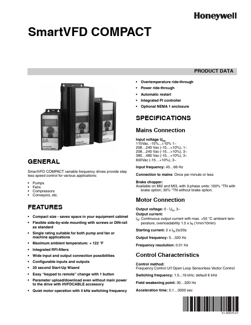
PRODUCT DATA31-00075-01SmartVFD COMPACTGENERALSmartVFD COMP ACT variable frequency drives provide step less speed control for various applications:•Pumps •Fans•Compressors •Conveyors, etc.FEATURES•Compact size - saves space in your equipment cabinet •Flexible side-by-side mounting with screws or DIN-rail as standard •Single rating suitable for both pump and fan or machine applications •Maximum ambient temperature: + 122 °F •Integrated RFI-filters•Wide input and output connection possibilities •Configurable inputs and outputs •30 second Start-Up Wizard•Easy “keypad to remote” change with 1 button •Parameter upload/download even without main power to the drive with HVFDCABLE accessory •Quiet motor operation with 4 kHz switching frequency•Overtemperature ride-through •Power ride-through •Automatic restart •Integrated PI controller •Optional NEMA 1 enclosureSPECIFICATIONSMains ConnectionInput voltage U in:115Vac, -15%...+10% 1~208…240 Vac (-15…+10%), 1~208…240 Vac (-15…+10%), 3~380…480 Vac (-15…+10%), 3~600Vac (-15…+10%), 3~Input frequency: 45…66 HzConnection to mains : Once per minute or lessBrake chopper:Available on MI2 and MI3, with 3-phase units: 100% *TN with brake option; 30% *TN without brake option.Motor ConnectionOutput voltage: 0 - U in , 3~Output current:I N : Continuous output current with max. +50 °C ambient tem-perature, overloadability 1.5 x I N (1min/10min)Starting current: 2 x I N 2s/20s Output frequency: 0…320 Hz Frequency resolution: 0.01 HzControl CharacteristicsControl method:Frequency Control U/f Open Loop Sensorless Vector Control Switching frequency: 1.5...16 kHz; default 6 kHz Field weakening point: 30…320 Hz Acceleration time:0.1…3000 secSMARTVFD COMP ACT31-00075—012Deceleration time: 0.1…3000 secBraking torque:100% *TN with brake option (only in 3~ drives sizes MI2 and MI3)30%*TN without brake optionAmbient ConditionsOperating temperature:+ 14 °F (-10 °C) (no frost)…+ 104/122 °F(40/50 °C) for 115 Vac, 460 Vac and 600 Vac and + 104 °F (40 °C), for 208 Vac/230 Vac, rated loadability I N Storage temperature: -40 °F (-40 °C)…+158 °F (+70 °C)Air quality :Chemical vapors:IEC 721-3-3, unit in operation, class 3C2Mechanical particles:IEC 721-3-3, unit in operation, class 3S2Altitude:100% load capacity (no derating) up to 1000 m1% derating for each 100 m above 1000 m; max. 2000 m Relative humidity:0…95% RH, non-condensing, non-corrosive, no dripping water Vibration: 3...150 HzEN50178, EN60068-2-6:Displacement amplitude 1(peak) mm at 3...15.8 Hz Max acceleration amplitude 1 g at 15.8...150 Hz ShockEN50178, IEC 68-2-27:UPS Drop T est (for applicable UPS weights)Storage and shipping: max 15 g, 11 ms (in package)Enclosure class: Open chassis, NEMA 1 kit optionalElectro Magnetic Compatibility (EMC)Immunity:Complies with EN50082-1, -2, EN61800-3, Category C2Emissions:115V: Complies with EMC category C4230V: Complies with EMC category C2; with an internal RFI filter400V: Complies with EMC category C2; with an internal RFI filter600V: Complies with EMC category C4All: No EMC emission protection (Honeywell level N): Without RFI filterSafety:For safety: CB, CE, UL, cULFor EMC: CE, CB, c-tick(see unit nameplate for more detailed approvals)Control connectionsAnalog input voltage:0...+10V , Ri = 200k Ω (min), Resolution 10 bit, accuracy ±1%, electrically isolated Analog input current:0(4)…20 mA, Ri = 200Ω differential resolution 0.1%, accuracy ±1%, electrically isolated Digital inputs: 6 positive logic; 0…+30 VDC Voltage output for digital inputs:+24V , ±20%, max. load 50 mA Output reference voltage :+10V , +3%, max. load 10 mAAnalog output :0(4)…20 mA; RL max. 500Ω; resolution 16 bit; accuracy ±1%Digital outputs :Relays:2 programmable relay outputs (1 NO/NC and 1 NO), Max.switching load: 250 Vac/2 A or 250 Vdc/0.4 A Open collector:1 open collector output with max. load 48 V/50 mAProtectionsOvervoltage protection:875VDC in HVFDCDXCXXXXXXX 437VDC in HVFDCDXBXXXXXXX Undervoltage protection:333VDC in HVFDCDXCXXXXXXX 160VDC in HVFDCDXBXXXXXXXEarth-fault protection:In case of earth fault in motor or motor cable, only the fre-quency converter is protected Unit overtemperature protection: YES Motor overload protection: YESMotor stall protection (fan/pump blocked): YES Motor underload protection(pump dry / belt broken detection): YES Short-circuit protection of +24V and +10V reference voltages: YESOvercurrent protection: T rip limit 4,0*I N instantaneouslySMARTVFD COMP ACT331-00075—01MODELSTable 1.Nominal Voltage Nom. HP (Nom. Current)EMC Filter Full IO (6DI, 2AI, 1AO,1DO, 3RO, Modbus)Frame Size: MI1Dimensions: 6.2" H x 2.6" W x 3.9" D460V3~in 3~out0.5 HP (1.3 A)No HVFDCD3C0005F00EMC HVFDCD3C0005F010.75 HP (1.9 A)No HVFDCD3C0007F00EMC HVFDCD3C0007F011 HP (2.4 A)No HVFDCD3C0010F00EMC HVFDCD3C0010F01208/230V 1~in 3~out 0.25 HP (1.7 A)EMC HVFDCD1B0003F010.5 HP (2.4 A)EMC HVFDCD1B0005F010.75 HP (2.8 A)EMC HVFDCD1B0007F01208/230V 3~in 3~out 0.25 HP (1.7 A)No HVFDCD3B0003F000.5 HP (2.4 A)No HVFDCD3B0005F00Frame Size: MI2 Dimensions: 7.7" H x 3.5" W x 4.0" D460V3~in 3~out1.5 HP (3.3 A)No HVFDCD3C0015F00EMC HVFDCD3C0015F012 HP (4.3 A)No HVFDCD3C0020F00EMC HVFDCD3C0020F013 HP (5.6 A)No HVFDCD3C0030F00EMC HVFDCD3C0030F01208/230V 1~in 3~out 1 HP (3.7A)EMC HVFDCD1B0010F011.5 HP (4.8 A)EMC HVFDCD1B0015F012 HP (7 A)EMC HVFDCD1B0020F01208/230V 3~in 3~out 1 HP (3.7A)No HVFDCD3B0010F002 HP (7 A)No HVFDCD3B0020F00115V/230V 1~in 3~out0.25 HP (1.7 A)No HVFDCD1A0003F000.5 HP (2.4 A)No HVFDCD1A0005F001 HP (3.7A)NoHVFDCD1A0010F00SMARTVFD COMP ACT31-00075—014PRODUCT IDENTIFICATION CODEFig. 1. Product Identification Code.Frame Size: MI3Dimensions: 10.2" H x 3.9" W x 4.3" D460V3~in 3~out4 HP (7.6 A)No HVFDCD3C0040F00EMC HVFDCD3C0040F015 HP (9 A)No HVFDCD3C0050F00EMC HVFDCD3C0050F017.5 HP (12 A)No HVFDCD3C0075F00EMC HVFDCD3C0075F01208/230V 1~in 3~out 3 HP (1 A)EMC HVFDCD1B0030F01208/230V 3~in 3~out 3 HP (11 A)No HVFDCD3B0030F00115V/230V 1~in 3~out 1.5 HP (4.8 A)No HVFDCD1A0015F00600V3~in 3~out1 HP (2 A)No HVFDCD3D0010F002 HP (3.6 A)No HVFDCD3D0020F003 HP (5 A)No HVFDCD3D0030F005 HP (7.6 A)No HVFDCD3D0050F007.5 HP (10.4 A)NoHVFDCD3D0075F00Nominal Voltage Nom. HP (Nom. Current)EMC Filter Full IO (6DI, 2AI, 1AO,1DO, 3RO, Modbus)SMARTVFD COMP ACT531-00075—01MECHANICAL DIMENSIONS AND MOUNTINGThere are two possible ways to mount the SmartDrive Compact onto the wall; either screw or DIN-rail mounting. The mounting dimensions are also given on the back of the inverter.Fig. 2. Mounting with screws or DIN-rail.Fig. 3. Dimensions in inches.Mechanical size H1H2H3W1W2W3D1D2MI1 6.2 5.8 5.4 2.6 1.50.2 3.90.3MI27.77.2 6.7 3.5 2.50.2 4.00.3MI310.39.99.53.93.00.24.30.3SMARTVFD COMP ACT31-00075—016COOLINGForced air flow cooling is used in all SmartDrive Compact drives. Enough free space shall be left above and below the inverter to ensure sufficient air circulation and cooling. SmartDrive Compact products can be mounted side by side. Y ou will find the required dimensions for free space and cooling air in the tables below:Table 2.Table 3.CABLING AND FUSESUse cables with heat resistance of at least +158 °F (+70 °C). The cables and the fuses must be dimensioned according to the following tables. The fuses function also as cable overload protection. These instructions apply only to cases with one motor and one cable connection from the inverter to the motor. In any other case, contact your Honeywell Sales Representative.Table 4.Table 5. Cable and fuse sizes for 208-240 V .Table 6. Cable and fuse sizes for 380-480 V .Mechanical size Free space above [inches]Free space below [inches]MI1 4.0 2.0MI2 4.0 2.0MI34.0 2.0Mechanical size Cooling air required [CFM]MI1 5.89MI2 5.89MI317.7Connection Cable typeMains cable Power cable intended for fixed installation and the specific mains voltage. Shielded cable not required. (NKCABLES/MCMK or similar recommended)Motor cablePower cable equipped with compact low-impedance shield and intended for the specific mains voltage. (NKCABLES /MCCMK, SAB/ÖZCUY -J or similar recommended). 360º grounding of both motor and FC connection required to meet the standards.Control cableScreened cable equipped with compact low-impedance shield (NKCABLES /Jamak, SAB/ÖZCuY -O or similar).Size Type (power)I N [A]Fuse [A]Mains cable Cu[AWG]Terminals cable size (min/max)Main terminal [AWG]Earth terminal [AWG]Control terminal [AWG]Relayterminal [AWG]MI1P25 - P751,7 – 3,710 2 x 15 + 1515 - 1115 - 1120 - 1520 - 15MI21P1 - 1P54,8 – 7,020 2 x 13 + 1315 - 1115 - 1120 - 1520 - 15MI32P211322 x 9 + 915 - 915 - 920 - 1520 - 15Size Type (power)I N [A]Fuse [A]Mains cable Cu[AWG]Terminals cable size (min/max)Main terminal [AWG]Earth terminal [AWG]Control terminal [AWG]Relayterminal [AWG]MI1P37 - 1P11,9 – 3,36 3 x 15 + 1515 - 1115 - 1120 - 1520 - 15MI21P5 - 2P24,3 – 5,610 3 x 15 + 1515 - 1115 - 1120 - 1520 - 15MI33P0 - 5P57,6 - 1220 3 x 13 + 1315 - 915 - 920 - 1520 - 15SMARTVFD COMP ACTFig. 4. SmartDrive Compact power connections.Fig. 5. SmartDrive Compact control connections wiring.Fig. 6. SmartVFD Compact control connection terminals.731-00075—01SMARTVFD COMP ACT31-00075—018The table below shows the SmartDrive Compact control connections with the terminal numbers.Fig. 7. Control inputs and outputs – API Full.FEATURES / FUNCTIONSEasy to set-up featuresTable 7.FeatureFunctionsBenefit30 second Start-up wizardSimple 4 step wizard for specific applications Activate wizard by pressing stop for 5 seconds Tune the motor nominal speed Tune the motor nominal currentSelect mode (0=basic, 1= Fan, 2 = Pump and 3 = Conveyor)Fully configured inverter for the application in question Ready to accept 0-10V analog speed signal in just 30 seconds“Keypad – Remote” OperationPush the navigation wheel for 5 seconds to move from remote control (I/O or Fieldbus) to manual mode and back.Single button operation to change the control tomanual (keypad) and back. Useful function whencommissioning and testing applicationsQuick Setup MenuOnly the most commonly used parameters are visible in basic view to provide easier navigation. The full view can be seen after P13.1 Parameter conceal is deactivated by changing the value to 0.Easy navigation through the most common parameters SmartVFD Commissioning Tool1.Parameter sets can be uploaded and downloaded with thistool.2.Easy to use PC-tool for commissioning the SmartVFD Invert-ers. Connection with HVFDCABLE and MCA adapter, (HVFD-CDMCAKIT/U), to the USB port of the PC. PC-tools available for download free of charge fromhttps:///en-US/support/commercial/software/vfds/Pages/default.aspxParameter copying easily from 1 inverter to another.Easy download of parameter sets created with PC-tool Parametering with PC Saving settings to PC Comparing parameter settingsSMARTVFD COMP ACT931-00075—01Compact and robust design with easy installationTable 8.Uninterruptible operation functionsTable 9.VFD and motor control featuresTable 10.OPTIONAL ACCESSORIESTable 11. SmartVFD COMPACT Accessories.FeatureFunctionsBenefitCompact size Minimum free space above and below the drive is required for cooling airflow.Minimum space requirementsIntegrated RFI-filtersThe units comply with EN61800-3 category C2 as standard. This level is the required level for public electricity networks such as buildings.Easy selection and installation of products.Space savingsCost savings Single power ratingSingle power suitable for both pump and fan or machine applicationsEasy selectionMax. ambient temperature + 122 °FHigh maximum ambient operating temperature Uninterruptible operationSide by side mounting with screws or DIN-rail asstandardSmartDrive Compact can be mounted side by side with no space between the units either with screws or on DIN-rail as standard.Dimensions for screw mounting can be found also on the back of the inverter.Easy installationSpace savings FeatureFunctionsBenefitOvertemperature ride-through Automatically adjusts switching frequency to adapt to unusual increase in ambientUninterruptible operationPower ride-through Automatically lowers motor speed to adapt to sudden voltage drop such as power lossUninterruptible operation Auto restart functionAuto restart function can be configured to make VFD restart automatically once fault is addressedUninterruptible operationFeatureFunctionsBenefitFlying startAbility to get an already spinning fan under speed control Improved performance Ease of application Inbuilt PI- controllerCapability to make a standalone system with sensor connected directly to the inverter for complete PI- control.Cost savingModel NumberDescriptionHVFDCABLE/U SmartVFD Commissioning Cable and USB Adaptor HVFDCDMCA/U Compact Commissioning Device HVFDCDMCAKIT/U Compact Commissioning Kit HVFDCDNEMA1FR1/U Compact NEMA 1 Kit Frame Size1HVFDCDNEMA1FR2/U Compact NEMA 1 Kit Frame Size2HVFDCDNEMA1FR3/U Compact NEMA 1 Kit Frame Size3HVFDCDTRAINER/UCompact Training Demonstration KitSMARTVFD COMP ACT31-00075—0110SMARTVFD COMP ACT 1131-00075—01SMARTVFD COMP ACTAutomation and Control Solutions Honeywell International Inc.1985 Douglas Drive North Golden Valley, MN 55422 ® U.S. Registered T rademark© 2015 Honeywell International Inc. 31-00075—01 M.S. 01-15 Printed in United StatesBy using this Honeywell literature, you agree that Honeywell will have no liability for any damages arising out of your use or modification to, the literature. You will defend and indemnify Honeywell, its affiliates and subsidiaries, from and against any liability, cost, or damages, including attorneys’ fees, arising out of, or resulting from, any modification to the literature by you.。

远距离激光光斑定位中的光晕抖动抑制算法

远距离激光光斑定位中的光晕抖动抑制算法邓凯鹏;陶卫;赵辉;金毅【摘要】In mechanical engineering, spatial location measurement in large spatial structure such as truss structure is generally required. Laser spot location method illuminates reflective marker with laser source and acquires the reflected laser spot with industrial camera. After detecting the edge of the spot with Canny detector, least square circle fitting will be led to get the fit spot center as the location of the marker. In long-distance location, Halo thrashing frequently occurs at the edge of laser spot. To restrain the trashing error and improve the precision of measurement, timing sequence filtering algorithm and quadratic fitting algorithm based on smooth filtering on time series value and refitting after removing noise are introduced in this paper to eliminate the effects of halo thrashing on measurement. The two algorithms are comparatively analyzed and verified by experiment of laser spot location of reflective target with distance as 12.36 m, and the repeatability error upper and lower limits are respectively optimized to ±0.22 pixel and ±0.26 pixel by the given algorithms, which are proved as effective for restraining the repeatability error caused by halo trashing.%在机械工程等领域，大型桁架等空间结构的空间定位需求十分普遍。

基于PB相位的等离子体超透镜设计

新技术新工艺2020年第8期基于PB相位的等离子体超透镜设计#夏习成，姚赞(中国科学技术大学精密机械与精密仪器系，安徽合肥230027)摘要：相较于传统光学透镜，超透镜具有对光的可操纵性强、设计灵活和易于集成化等众多优点。

然而基于电介质的超透镜需要亚波长尺度的高深宽比结构，对加工技术要求十分苛刻&提出了一种基于PB相位的等离子体超透镜设计方式,通过控制结构单元光轴方向可以实现对圆偏振光的调控，设计中采用的在金膜上刻蚀矩形孔的方式可以大大降低对加工条件的要求。

基于时域有限差分(FDTD)的仿真计算表明，超透镜的焦距与设计值偏差约为2.5%，焦点半高宽(FWHM)与衍射极限偏差约为2.7%，具有较好的吻合度。

关键词：超表面；超透镜；相位调控；PB相位；时域有限差分；圆偏振光中图分类号:TH74文献标志码:ADesign of Plasma Metalens Based on PB PhaseXIA Xicheng,YAO Zan(Department of Precision Machinery and Instrumentation,University of Science and Technology of China,Hefei230027 ,China) Abstract:Compared with traditional optical lens,the metalens had many advantages such as strong maneuverability to light ,flexible design,easy integration and so on.However,dielectric-based metalens required a high aspect ratio structure atthesub-wavelengthscale whichdemandedhighprocessingtechnology APBphase-basedplasmametalensdesignmethod wasproposed bycontro l ingthedirectionoftheopticalaxisofthestructuralunit itwaspossibletoadjustthephaseofthe circularly polarized light,the method of etching rectangular holes in the gold film used in this design could greatly reduce pDocessingDequiDements.The simulation calculation based on finite di f eDence in time domain(FDTD)showed that the devi-ationofthefocallengthofthemetalensfDomthedesignvaluewasabout2.5%and the deviation between the FWHM with thedi D actionlimitwasabout2.7%ithadagoodagDeement.Keywords:metasuDface metalens phasecontDol PBphase finitedi f eDenceintimedomain ciDculaDlypolaDizedlight传统的聚焦透镜对光线的调控依赖于沿着光路的相位积累,因此会受到自然材料折射率的限制’此外,对制造工艺的要求也会很高,想要加工高精度的透镜十分困难’超表面的优越特性吸引了国内外学者的极大兴趣,其概念最早由Yu等提出，他们提出了一种V形纳米天线组成的超表面山，通过改变天线的开口方向可以实现对圆偏振光的调控,并提出了广义斯涅尔定律来解释。

ARRI L-Series LED Fresnel 产品介绍说明书

Tuneable Tungsten allows for fine-tuning of thetungsten color temperature from 2,600 K to 3,600 K with increased brightness over the L7-C, and is particularly suited to applications requiring precise matching to conventional tungsten lampheads.Color temperature, tint and hue can becontinuously adjusted from 2,800 K to 10,000 K, between full plus or minus green and RGBW colors.Tuneable Daylight allows for fine-tuning of the daylight colortemperature from 5,000 K to 6,500 K with increased brightness over the L7-C, and is particularly suited to applications requiring precise matching to daylight balanced light sources.UNIQUE LED LIGHTS WITH TRUE FRESNEL PERFORMANCEThe ARRI L-Series is an LED Fresnel fixture so close to its conventional counterpart in function and performance that it creates a previously unattainable o pportunity: l ike-for-like r eplacement of traditional Fresnels with LED-based units.The L7 is the first LED fixture to truly incorporate the Fresnel characteristics ofcontinuous focusability from spot to flood and a smooth, homogenous light field. The L-Series takes full advantage of LED technology and allows for complete control over the color and intensity of light. Light emitted from the L7 is specifically calibrated for optimal reproduction on broadcast and digital cinema cameras, ensuring pleasing skin tones and vividly rendered colors. Constructed to be robust and ergonomic, the L7 meets the quality and design standard for which ARRI is known.The most recent addition to the L7 line is a brighter L7-C. Taking advantage of advancements in LED technology, the L7-C is now 25 % brighter than perviousversions. With the new Light Engine 2, the L7-C is more versatile than ever before. The LE2 (Light Engine 2) now comes standard withevery L7-C. An upgrade for L7-Cs with LE1 is also available.ALL VERSIONS INCLUDE the following base configurations: powerCON TRUE1 Mains Cable, Onboard control panel, 5-Pin DMX In and Thru connector, 28 mm spigot (1 1/8”) Junior PinHANGING versions include the following base configuration: 1.5 m (5 ft) Mains Cable with bare endsPOLE-OPERATED versions include the following base configuration: 1.5 m (5 ft) Mains Cable with bare ends, Pole Operation for pan, tilt and focusSTAND-MOUNT versions include the following base configuration: 3 m (10 ft) Mains Cable with Schuko connector and line switchNOT INCLUDED: Barndoors (have to be ordered separately)approx. 15 % brighter than L7-Capprox. 15 % brighter than L7-COrder No.DescriptionL0.0015232L7-C, LE2, Hanging, Blue/Silver L0.0015217L7-C, LE2, Hanging, Black L0.0015234L7-C, LE2, Pole Operated, Blue/Silver L0.0015216L7-C, LE2, Pole Operated, Black L0.0015233L7-C, LE2, Stand-Mount, Blue/Silver, 3 m Cable, Schuko Connector L0.0015336L7-C, LE2, Stand-Mount, Blue/Silver, 7 m Cable, Edison ConnectorOrder No.DescriptionL0.0015225L7-TT, Hanging, Blue/Silver L0.0015231L7-TT, Hanging, Black L0.0015228L7-TT, Pole Operated, Blue/Silver L0.0015230L7-TT, Pole Operated, Black L0.0015227L7-TT, Stand-Mount, Blue/Silver, 3 m Cable, Schuko Connector L0.0015340L7-TT, Stand-Mount, Blue/Silver, 7 m Cable, Edison ConnectorOrder No.DescriptionL0.0015218L7-DT Hanging, Blue/Silver L0.0015223L7-DT Hanging, Black L0.0015220L7-DT Pole Operated, Blue/Silver L0.0015222L7-DT Pole Operated, Black L0.0015219L7-DT Stand-Mount, Blue/Silver, 3 m Cable, Schuko Connector L0.0015338L7-DT Stand-Mount, Blue/Silver,7 m Cable, Edison ConnectorPhotometric Data (nominal results)Spot: 15°8522 lx / 792 fc 3068 lx / 285 fc 1565 lx / 145 fc 947 lx / 88 fc Middle: 30°2444 lx /227 fc 880 lx / 82 fc 449 lx / 42 fc 272 lx / 25 fc Flood: 50°1031 lx / 96 fc 371 lx / 34 fc189 lx / 18 fc115 lx / 11 fcOptical System Focusable Fresnel Lens Diameter 175 mm / 7“Beam Angle 15° to 50° (Half Peak Angle)Weight Manual Version: 8.7 kg (19.2 lbs) Pole Op Version: 10.1 kg (22.3 lbs)Handling Adjustable Sliding Stirrup, High Strength Tilt Lock, Pole Operation Option (Pan, Tilt and Focus)Mounting 28 mm Spigot (Junior Pin)Tilt Angle+/- 90°Power Supply Range 100 to 250 V ~, 50/60 HzPower Consumption L7-C & L7-TT: 160 W Nominal, 220 W Maximum L7-DT: 180 W Nominal, 220 W MaximumPower Connection powerCON TRUE1 (Bare Ends / Schuko / Edison Cables Available)White LightL7-C: 2,800 K to 10,000 K Continuously Variable Correlated Color Temperature L7-TT: 2,600 K to 3,600 K Continuously Variable Correlated Color Temperature L7-DT: 5,000 K to 6,500 K Continuously Variable Correlated Color Temperature Colored Light (L7-C only)Full RGB+W Color Gamut with Hue and Saturation Control Color Temperature Tolerance +/- 100 K (nominal), +/- 1/8 Green-Magenta (nominal)Color RenditionL7-C: CRI Average >94, TLCI Average >90L7-TT: CRI Average >94L7-DT: CRI Average >92Green-Magenta Adjustment Continuously Adjustable (Full Minusgreen to Full Plusgreen)Dimming 0 to 100 % continuousControl5-Pin DMX In and Through, On-Board Controller, Mini-USB Remote Device Management (RDM)DMX Setup, Hour Counter and Standard RDM CommandsMini-USB Interface DMX Setup, Fixture Status and Firmware Upgrade Through PC Software Housing ColorBlue/Silver, Black Ambient Temperature Operation -20 to 45º C (-4 - 113º F)Protection Class / IP Rating I / IP20Estimated LED Lifetime (L70)50,000 hours Estimated Color Shift Over Lifetime (CCT)+/- 5 %CertificationsCE, CB, GS, cNRTLus, FCC, PSEAll specifications are nominal / typical values.Technical Specifications。

2005年诺贝尔物理学奖与光学频率梳

评述
2005年诺贝尔物理学奖与光学频率梳 3
魏志义
(北京凝聚态物理国家实验室中国科学院物理研究所光物理实验室北京 100080)
摘要光学频率梳是 2005年诺贝尔物理学奖的重要内容 ,本文结合时间频率标准的发展历史 ,简要介绍了飞秒频率梳的基本原理、发明背景、科学意义及研究趋势. 最后通过对该项发明的思考 ,浅谈了一点对科学研究方法的不成熟认识. 关键词 2005年度诺贝尔物理学奖 ,光学频率梳 ,飞秒激光脉冲
Abstract The development of op tical frequency comb technique greatly pushed the revolutionary p rogress in laser - based p recision spectroscopy, which shared the 2005 Nobel p rize in physics. Following the history of time - frequency standard, the basic p ricinp le and background of op tical frequency comb techniques are re2 viewed in this paper, the app lications and the latest research activities are also briefly introduced. Finally, based on the analysis on the inventive work, I give some simp le comments on the style of scientific research. Keywords 2005 Nobel p rize in physics, op tical frequency comb, fem tosecond laser pulse

2005年诺贝尔物理学奖与光学频率梳

The 2005 Nobel pr ize in physics and optica l
frequency com b techn iques
W E I Zhi2Yi
( B eijing N a tional L aboratory for Condensed M a tter Physics, Institute of Physics, Ch inese A cadem y of S ciences, B eijing 100080, Ch ina)
评述
量级的飞秒激光展宽到大于一个倍频程 ,即同时包含有基波波长与倍频波长的超宽光谱 ,而且利用色散补偿技术将脉冲宽度压缩到了 5fs[7 ]. 在这样短的时间内 ,根据光传输距离与时间的关系 τ=λ/ c, 800nm 载波波长的激光所能振荡的时间还不到 2个光周期. 对于这样短的激光脉冲 ,一个需要认真考虑的问题是其载波与脉冲包络之间的相位 ( carrier envelope phase, CEP)变化情况. 就在这一年 ,时在维也纳技术大学访问研究的中国科学院西安光机所青年学者许林与亨
2005年诺贝尔奖的评选与授奖活动已落下帷幕 ,三名科学家由于在与光学相关的研究领域所做出的杰出成就而获物理学奖的殊荣 ,其中美国哈佛大学的格劳伯教授 (R. J. Glauber)因对“光相干性的量子理论 ”的贡献而分享该奖的一半 ,另一半由美国国家标准技术研究院 (N IST) 的霍尔教授 ( J. L. Hall)和德国马普量子光学所 (M PQ )的亨施教授 ( T. W. H nsch)共同获得 ,以奖励他俩对“超精细激光光谱学 ,包括光学频率梳技术 ”的贡献. 作为该年度物理学奖的重要内容 ,光学频率梳对许多人而言也许是一个新名词 ,那么其究竟表达了一种什么样的物理概念 ? 在该项诺贝尔奖中起着什么样的作用 ? 本文从笔者粗浅的理解角度 ,简单介绍光学频率梳的出现、发展以及重要应用.

光学仪器测量方法：镜面间距检测系统说明书

8th International Conference on Manufacturing Science and Engineering (ICMSE 2018)Design Method of the Measuring System for the Mirror Surface Spacingof a compound lensPing Zhong1,a,Shaohui Pan1,b, Zhisong Li2,c and Xingyu Gao1,d1College of Science, Donghua University, Shanghai 201620, PR China2College of Information Science and Technology, Donghua University, Shanghai 201620, PR China a b*****************,c****************,d*****************Keywords:Optical fiber low coherence interference, lens mirror space, Signal-to-noise ratio, Band-pass filter, least square methodAbstract:Based on the principle of low coherent light interference of optical fiber, a new method for detecting the distance between the mirror surfaces of a compound lens is proposed. Firstly, a system based on the principle of low coherent light interference is designed. Secondly, the frequency calculation method of interference signal of measurement system is put forward, and the band-pass filter is designed for interference signal to improve the signal-to-noise ratios. Based on the characteristics of low coherence light interference signal, the least squares symmetric peak location algorithm is proposed, which realizes the precise locating of the peak of the interferometric signal. Besides, the experiment of measuring the distance between the compound lens is carried out and the measurement error is analyzed.IntroductionIn the manufacture of optical instruments, the center thickness machining precision and assembly precision of the lens have an important influence on the imaging quality of the optical system. Especially in high-performance precision optical systems such as aviation, aerospace and microscope systems, there are strict control requirements for the lens center thickness and the mirror spacing. So, how to get high precision measurement results is a challenging topic. At present, the method for measuring distance between the mirror surfaces of a compound lens is mainly divided into two types, the one is contact measurement and the other is non-contact measurement. The structure of contact measurement is relatively simple, but it has a large defect itself, such as easy to scratch the lens and destroy the lens. The frequent contact between the surfaces of the probe and lens can also make the worn lenses and affect the measurement accuracy. Non-contact measurement system is relatively complex, but it can perform nondestructive testing on the lens group. It is mainly to measure the relative position of the mirror surface by measuring the reflection signal of the lens surface. The methods mainly include image method [1], axial dispersion [2], differential confocal method [3], image calibration method [4, 5], etc. Low-coherence optical interferometry, as the main detection method of non-contact measurement for optical devices, is one of the hotspots today. In this paper, based on the principle of low-coherence light interference, a system for measuring the lens spacing of the compound lens is designed and the main factors affecting the detection accuracy are studied, and the effective method for signal filtering and waveform peak location is proposed.Measurement principle and system design of lens spacingLow-coherence light interferometry [6-12] is an interferometric technique using a broad-spectrum light source as a coherent light source. The coherence length is short and the interference peak can be generated only when the optical path of the measured light and the reference light is equal, so it has a good spatial positioning characteristic. By calculating the distance between the interference peaks at the apex of the front and rear mirror surfaces, the lens group spacing and the center thickness of the lens can be calculated. In this paper, the basic structure of Michelson interferometer is adopted, in which the light emitted the light source is passed through the optical fiber coupler to produce the measured light and the reference light respectively. On the one hand, the reflected signal come from the different surfaces of the sample has a different optical path. On the other hand, the referenceCopyright © 2018, the Authors. Published by Atlantis Press.This is an open access article under the CC BY-NC license (/licenses/by-nc/4.0/). 649optical path will change with the position of the reference mirror. Only the reflected signal from a specific location of the sample can be coherent with the reference light, where the location of the maximum intensity of coherent signal corresponds to the equal optical path position. The structure of the lens spacing measurement system is designed as shown in Fig.1.Fig.1. Lens group spacing detection system diagramThe light emitted from the wide-spectrum light source SLD (center wavelength 1310 nm, half-wave width 85 nm) is split by the fiber coupler and then enters the circulator 1 and the circulator 2, and forms measurement light and reference light, respectively. In order to facilitate the installation and debug the detection system, the visible light with the wavelength of 660nm and the measured light are mixed in the wavelength division multiplexer, and then, they are projected onto the front and back surfaces of the lens group by the collimator and reflected by the front and back surfaces of the lenses in the compound lens. Finally, the reflected light is shot into the ring through the collimator and the wavelength division multiplexer and recoupled into the optical fiber system from the port 3. In the same way, the reference light is reflected by a movable plane reflector. The returned reference light is ejected through port 3 of the ring and interferes with the measured light in the optical fiber coupler. The returned reference light is ejected through port 3 of the ring and interferes with the measured light in the optical fiber coupler. The path of the reference light can be changed by driving a plane reflector to move uniformly in a straight line. When the optical path of the measured light is equal to that of the reference light, that is, when the optical path difference is zero, the interference signal is strongest, at this time the maximum wave peak signal can be detected by the computer.Since the measuring beam contains many light rays reflected from the front and rear surfaces of multiple lenses, there will be multiple sets of maximum wave peaks in the process of moving plane reflector. According to the relative position of two zero light path difference, the measurement of lens spacing of compound lens can be completed. In the process of measurement, the information of the plane reflector is recorded in real time by a high resolution grating scale displacement sensor. In order to suppress the common-mode noise of the system and improve the signal-to-noise ratio of the system as much as possible, the system proposed in this paper uses a balanced detector for the photoelectric conversion of the interference signal. Then the data acquisition card is controlled by the computer, and the signal is processed by the computer. In order to further suppress the noise, a signal filter is designed.Signal filtering and waveform peak locationDesign of band-pass filterIn the detection system, the intensity of reflected light of the plane mirror is higher than the intensity of the tested lens. When the intensity ratio of the incident light passing through the reference light and detection light is 50:50, the interference signal is very weak. Fig.2(a) shows the waveform of the interference signals. In this case, the peaks of interference signals are difficult to extract. Through experiments, we can set the intensity ratio of the incident light passing through the reference light and detection light as 80: 20, and the output interference signals are very obvious as shown inFig.2(b).650Fig.2. The comparison of interference signal intensity.(a) the waveform of the interference signals while theintensity ratio is 50:50; (b) the waveform of the interference signals while the intensity ratio is 80:20It can be seen from Fig.2 (b) that, although the strong contrast interference signal can be obtained by setting the light intensity ratio between the reference light and detection light, the interference signal are often mixed with noise, which directly affects the location of peak signal. In this paper, a band-pass filter is designed to suppress the noise signal and improve the signal-to-noise ratio [13,14].The center wavelength of the designed filter can be calculated. Assuming that the moving speed of the plane mirror on a guide rail is mm/s during detection process and the center wavelength of the broadband light source is λ nm, then the center wavelength ( f ) of the filter can be calculated by the Eq.(1):=(2 ∕ )×10 . (1)For the system designed in this paper, v is 3.78mm/s , the wavelength rang of the broadband light source is 1290∼1330 nm, λ is 1310nm , thus the f =5.77×10 kHz and the frequency range of a band-pass filter is from 4.77kHz to 6.77kHz , and the center frequency can be selected as 5.77kHz .Method for locating the peak of interference signalIn this paper, the location of the peak of interference signal is the key to detection of lens spacing and can be determined by extracting the signal envelope. According` to the principle of low coherence interference, the wave peak of interference signal represents the interference generation between the reference light and detection light at zero optical paths. For measuring system, as long as the optical path difference between the two peaks of the interferometric signal from the lens group is obtained, the distance between the lenses of compound lens can be obtained. A simple method is to use the peak signal to determine the location of the zero optical path difference. However, because the adjacent extreme signals are so close to each other, the noise introduced in the detection process can easily cause location error which will lead to poor repeatability accuracy of the measurement system. The Gauss fitting algorithm has the advantage of locating peaks, but it requires that the interference signal has good symmetry. So it cannot meet the requirements of the system designed in this paper. In this paper, a symmetric peak location algorithm based on the least square method is proposed.First, the acquired interference signals are preprocess. Fig.3(a) shows the primary signals collected. The position of the mean value of the intensity is set to the abscissa axis. Fig.3(b) shows the sum of the absolute values for the same position signals. The envelope image of the signals is represented by a dotted line shown in Fig.3(b).According to the theory of partial coherence, when the value of function of the location points in envelope curve is greater than 1/e of the maximum value, these points are directly related to the coherence length of the light source. So the signals whose value is greater than 1/e of the maximum value point are selected as an effective processing signal, and then the location of peak signal can bedetermined by the a symmetric peak location algorithm based on least square. 651Fig.3. The method of locating signal peak.(a) The primary signals collected; (b) Envelope image of signal The method can be described as follows: i) Firstly, all points whose values are greater than 1/e of the maximum are selected, and then these points are plotted as a curve which called the original curve, it can be seen in Fig.4(a). After that, a symmetry axis which is parallel to the vertical axis and passes through the maximum value point of the original curve is drawn, then, the original curve revolves around the symmetry axis and forms another curve which is called revolved curve. ii) The revolved curve is moved left or right along the horizontal axis. Meanwhile, the mean square error between the original curve and the revolved curve is calculated. When the mean square error obtained is the smallest, the best translational position to the revolved curve is determined. iii) The revolved curve was moved according to the translation amount, as shown in Fig.4(b). Finally, the symmetrical position of the two curves is used as the zero-path difference position. The method utilizes the least squares method can equalize the errors brought by the interference signals and the measurement error and the system error can be effectively reduced.Fig.4. The method of locating wave crests.(a) Flip chart; (b) Flipping the curve after translationSpecular distance measurement experiment and error analysisAccording to the design principle of lens spacing detection system, a measurement system is set up as shown in Fig.5. Among them, the center wavelength of the detection system is 1310nm, and the half wavelength width of the SLD wide spectrum light source is 85nm, and its optical power is 10.8mW.Fig.5 Measurement test system for detecting the distance between the mirror surfaces of a compound lens (1) a wave division multiplexer, (2) Circulator 1, (3) 80/20 fiber couplers, (4) Circulator 2, (5) 50/50 opticalcouplers, (6) the single mode fiber , (7) balance detector652In order to test the measurement accuracy of the system designed in this article, an achromatic composite lens group is selected to perform experiment for detecting distance between the mirror surfaces. Among them, the compound lens includes 7 groups of lenses, and the structure of the combined lens is shown in Fig.6.Fig.6 The structure of the lens group to be measuredAccording to the experimental system and the detection algorithm, the measurement of the lens spacing of the compound lens is carried out. The interference signal improvement is very obvious, and the output interference signal waveform was shown in Fig.7(a), and Fig.7(b) is the waveform of the interference signal after filtered.Fig.7 Measurement of the waveforms of the interferometric signal in the lens group, (a) the waveforms of theinterfering signal before filtering,(b) the waveforms of the interfering signal after filteringIn order to evaluate the accuracy and stability of the test system, the lens group has been measured for many times. Table.1 lists the design values of the measured lenses, the average values of the ten measurements and the standard deviation calculated.Table.1 Measurement data of spacing thickness of lens groupSampleDesign thickness or spacing[mm] The mean value of measuring thickness or spacing [mm] Standard deviation[nm] Lens 15 .00 5.0327 59 Air gap 1-26.00 6.0155 101 Lens 25.00 4.9879 127 Air gap 2-35.00 5.0214 167 Lens 36.00 5.9897 201 Air gap 3-45.90 5.8591 221 Lens 46.00 6.0319 260 Air gap 4-58.00 7.9981 239 Lens 55.00 4.9794 327 Air gap 5-618.00 17.8951 389 Lens 65.00 5.0124 372 Air gap 6-77.00 6.9978 408 Lens 77.00 7.0214425 653According to the results of the measurement data, it can be seen that the relative intensity of the reflected light on the lens surface at the rear end of the lens group is weak and the standard deviation of measurement is relatively large due to the influence of the number of lenses contained a compound lens and the reflection loss of the lens surface. With the increase of the number of lens to be measured, the interference signal gradually get weakened and the precise of the positioning accuracy of the zero optical path difference position be reduced，which will lead to an increase in the measurement standard deviation in measuring the lens spacing of the compound lens.ConclusionIn this paper, based on the low coherent light interference method, a system for measuring the lens spacing of the compound lens is designed. A calculation method of interference signal frequency in measurement system is put forward, and a bandpass filter is designed, which can effectively improve the signal-to-noise ratio of the interferometric signal. The fitting method of the interference signal envelope is proposed. Based on the characteristics of the low-coherence interference signal, we used a least-squares correction information positioning method, which effectively improves the repeatability of the measurement. Finally, by testing the lens spacing of the combined lens, the effectiveness of the proposed design method is proved. The detection system not only is convenient, fast, and has no damage to optical devices, but also has high precision and strong stability. It has a good application prospect in optical processing and optical detection.AcknowledgementsThis work is supported by the National Natural Science Foundation of China (Grant No.51575099)References[1] A.V. Goncharov, L.L. Bailon and N.M. Devaney. Spie:Vol.7389(2009),p.738912.[2] M. Kunkel, J. Schulze. Glass Science and Technology: Vol.78(2005),p.245.[3] L.B. Shi, L.R. Qiu and Y. Wang. Chinese Journal of Scientific Instrument :Vol. 33(2012),p. 683.[4] H.W. Gao, H. Wang, Y.Y. Liu and Y. Yu. Journal of Electronic Measurement and Instrument:Vol.31(2017),p.820.[5] J.H. Zhang, Q Liu and R.H. Nie.Spie:Vol.36(2016),p.174.[6] P. Langehanenberg,A. Ruprecht. Spie:Vol.8844(2013),p.88444F.[7] J. Benitez, J. Mora.IEEE Photonics Technology Letters:Vol.29(2017),p.1735.[8] S. Merlo, P. Poma and E. Crisa. Sensors:Vol.17(2017).[9] O. Martinez-Matos, C. Rickenstorff and S. Zamora. Optics Express:Vol.25(2017),p.3222.[10] R. Abuter, M. Accardo and A .Amorim. Astronomy & Astrophysics:Vol.602(2017).[11] R.W Kunze, R. Schmitt. Tm-Technisches Messen:Vol.84(2017),p.575.[12] K.Li, M. Jiang, Z.Z. Zhao and Z.M.Wang. Optics Communications:Vol.389(2017),p.234.[13] J.M.Tang, H.W. Liu, Q.F. Zhang, B.P. Ren and Y.H. Liu. IEEE Transactions on AppliedSuperconductivity:Vol.28(2018).[14] H Lu, Z.Q. Yue and J.L. Zhao. Optics Communications:Vol.414(2018).654。

星载激光测距合作目标的光学设计

第30卷第1期2004年1月光学技术OPTICAL TECHN IQU E Vol.30No.1Jan.　2004文章编号:100221582(2004)0120048203星载激光测距合作目标的光学设计Ξ聂辉1,翁兴涛1,李松1,刘基余2(1.武汉大学电子信息学院,武汉　430079;2.武汉大学测绘科学与技术学院,武汉　430079)摘　要:运行于空间轨道的角反射器由于受相对速度的影响,必须进行速差补偿。

针对轨道高度为20000km 的角反射器,确定了能够接受的直角面平面度;针对几何光学方法速差补偿的不准确,运用衍射原理,对速差补偿的效果按角差的不同进行搜索,得到了比较理想的结果,确定了角反射器的参数。

关键词:角反射器;速差补偿;两面角偏差;远场衍射中图分类号:V241.62+1;P228.5 文献标识码:AOptical design of the retro 2reflector in space for laser rangingNIE Hui 1,WE NG X ing 2tao 1,LI Song 1,LI U Ji 2yu 2(1.School of Electronic Information ,Wuhan University ,Wuhan 430079,China )(2.School of G eodesy and G eomatics ,Wuhan University ,Wuhan 430079)Abstract :A kind of satellite 2borne retro 2reflector in 20000km high orbit is optically designed.The far field diffraction pat 2terns of the cube corner prism with flatness error of back faces as well as dihedral an gle offsets are computed so that these error parameters are properly determined in order to com pensate the velocity aberration.It is shown that result derived from wave o p 2tics is different from that of geometrical optics and the physical optics provides the better and more rational a pproach to designing this cooperative target.K ey w ords :retro 2reflector ;velocity aberration compensation ;dihedral angle offset ;far field diffraction patterns0　引　言角反射器具有三个反射面和三个两面直角,由于角反射器的这种特殊结构,入射到角反射器的光束将按原光路返回。

光纤光学频率梳

光纤光学频率梳谢戈辉;刘洋;罗大平;朱志伟;邓泽江;顾澄琳;李文雪【摘要】在时域上,光学频率梳(光频梳)表现为时间间隔固定的超短脉冲序列,具有飞秒量级的时间宽度和极高的瞬时电场强度;在频域上,光频梳呈现为数百万频率间隔固定的频率齿的集合,每根梳齿都具备窄线宽稳频连续激光器的频率精度.光频梳已经发展成为一种重要的科研工具,广泛应用于高精度原子、分子特征信息识别,物质内部结构解析,生物成像及空间遥感成像等诸多科学研究领域.文章首先说明光频梳的基本技术原理,然后介绍华东师范大学精密光谱科学与技术国家重点实验室在光频梳研制领域的进展,并详细介绍基于自研光频梳发展的两种应用:双光梳三维编码成像和双光梳分子光谱.【期刊名称】《自然杂志》【年(卷),期】2019(041)001【总页数】9页(P15-23)【关键词】光学频率梳;飞秒锁模激光器;载波包络相位频率;重复频率;f-2f自参考探测技术;锁相环【作者】谢戈辉;刘洋;罗大平;朱志伟;邓泽江;顾澄琳;李文雪【作者单位】华东师范大学精密光谱科学与技术国家重点实验室,上海200062;华东师范大学精密光谱科学与技术国家重点实验室,上海200062;华东师范大学精密光谱科学与技术国家重点实验室,上海200062;华东师范大学精密光谱科学与技术国家重点实验室,上海200062;华东师范大学精密光谱科学与技术国家重点实验室,上海200062;华东师范大学精密光谱科学与技术国家重点实验室,上海200062;华东师范大学精密光谱科学与技术国家重点实验室,上海200062【正文语种】中文1 光学频率梳——时频域精密控制的飞秒激光脉冲20世纪后期，超快激光技术的快速发展为精密光谱测量技术提供了崭新的技术手段。

具有超高时间分辨能力的飞秒脉冲，赋予科研人员探索超快物理规律，获取原子、分子特征信息，认识物质内部能量传递的能力。

在工业生产方面，飞秒脉冲具有极高的峰值功率密度，最大限度地减小了热损伤，带来了前所未有的加工精度。

基于二维小波变换的圆形算子虹膜定位算法

基于二维小波变换的圆形算子虹膜定位算法赵静【摘要】An improved iris localization algorithm of circular operator based on two-dimensional wavelet transform is proposed to im-prove the accuracy and the speed of the iris localization. Firstly,the algorithm segments the pupil area of the iris by the threshold. Second-ly it locates the iris inner edge by the edge detection operator in the pupil area. Thirdly the human eye iris image is processed by the two-dimensional wavelet transform to reduce the image resolution instead of the smoothing function in the Daugman circular operator. Finally it gets the circular edge of the sliding window by the circular edge detection operator,and compares the circle inside mean gray with the circle outside mean gray to locate the iris outer edge. The simulation results show that the algorithm locates the iris inner and outer edge with 1. 85s average time and 99. 6% accuracy rate. The algorithm has a higher practical value in the iris recognition system.% 为了提高虹膜定位的准确率和速度,提出了一种基于二维小波变换的Daugman圆形算子虹膜定位改进算法。

船舶运动图像快速位移补偿方法简

船舶运动图像快速位移补偿方法罗菁晶(四川交通职业技术学院，四川温江 611130)摘要: 为了提高船舶运动成像的电子稳像能力，进行运动图像位移补偿处理，提出基于相邻帧多尺度补偿的船舶运动图像快速位移补偿方法，对采集的原始船舶运动图像采用小波降噪方法进行图像降噪处理，对降噪的船舶运动图像进行多尺度的经验模态分解，结合运动图像相邻帧的像素特征进行电子稳像补偿，根据电子稳像输出结果进行图像位移的快速补偿，提高船舶运动图像的成像质量。

仿真结果表明，采用该方法进行船舶运动图像位移补偿，对运动帧的连续成像效果较好，输出图像的峰值信噪比较高，表明对船舶运动图像的成像质量较高，能克服快速位移对运动图像成像质量的影响。

关键词：船舶运动图像；电子稳像；小波降噪；经验模态分解中图分类号：TP391 文献标识码：A文章编号： 1672 – 7649(2018)2A – 0166 – 03 doi：10.3404/j.issn.1672 – 7649.2018.2A.056Fast displacement compensation method for ship motion imageLUO Jing-jing(Sichuan Vocational and Technical College of Communications, Wenjiang 611130, China)Abstract: In order to improve the electronic image stabilization ability of ship motion imaging, motion image displace-ment compensation processing, a method of fast displacement compensation for ship motion images is proposed based on multi scale compensation of adjacent frames, wavelet denoising method of the original ship motion image acquisition using in image denoising, image denoising of the empirical mode of ship motion multi scale decomposition, combined with the characteristics of motion pixel images of adjacent frames of video stabilization compensation, according to the electronic im-age stabilization fast compensation output displacement image, improve the image quality of ship motion image. The simula-tion results show that using the method of ship motion image displacement compensation, better imaging effect of continu-ous motion frame, output the image of the high peak signal to noise ratio, shows that the ship motion image quality is higher, it can overcome the rapid displacement of motion image into like the effect of quality.Key words: ship moving image；electronic image；wavelet denoising；empirical mode decomposition0 引　言图像处理技术的发展对运动图像成像质量要求越来越高，结合电子稳像方法提高图像成像质量，克服因图像采集目标位移和抖动造成图像失稳的问题，优化成像。

211018260_高精度低时延CORDIC算法

现代电子技术Modern Electronics Technique2023年4月1日第46卷第7期Apr.2023Vol.46No.70引言现代数字通信系统对傅里叶变换、三角函数、双曲函数等运算的高性能硬件实现结构的需求日益迫切[1⁃2]。

CORDIC （Coordinate Rotation Digital Computer ）算法是一种规则化算法，它能够只通过移位与加减操作实现上述运算[3⁃4]，其具有可移植性强、电路结构简单的特点，适用于现场可编程门阵列、专用集成电路等设计场合，因而受到众多科研单位的广泛研究，是当前重要的研究热点之一[5⁃6]。

随着数字集成化电路对CORDIC 算法的性能要求不断提高，国内外众多学者对其进行了相应的改进与优高精度低时延CORDIC 算法揭灿，朱晓宇，赵霁（中国电子科技集团第五十八研究所，江苏无锡214000）摘要：针对目前流水线型坐标旋转数字计算机（CORDIC ）算法存在输出精度较低、输出时延较长的问题，提出一种基于移位相加结构的CORDIC 算法。

此算法首先对[0，π4）内的输入角度采用角度二极化重编码技术，将角度二进制编码转化为1和-1编码，然后使用移位相加结构替代查找表，同时通过合并迭代结构合并旋转迭代，减少迭代单元级数和迭代次数，降低硬件资源的消耗，建立小容量正余弦值ROM 表，降低接近于π2时部分输入角度的运算误差，最后结合角度区间映射手段保证算法运算范围覆盖整个圆周[0，2π）。

在Xilinx 公司KC705评估套件上进行算法验证与仿真，结果表明：在输出位宽都设定为16位的条件下，运算结果的绝对误差和相对误差相比流水线型CORDIC 算法分别降低了46.7%，83.5%，该算法只需6个时钟周期即可输出计算结果，输出时延减少了60.0%。

设计的CORDIC 算法具有输出精度高、输出时延短的优势，适用于实时、高精度的现代通信系统。

关键词：坐标旋转数字计算机；角度二极化重编码；移位相加；合并迭代；角度区间映射；数字信号处理中图分类号：TN492⁃34；TN914.3文献标识码：A文章编号：1004⁃373X （2023）07⁃0171⁃05CORDIC algorithm with high accuracy and low delayJIE Can ，ZHU Xiaoyu ，ZHAO Ji（The 58th Research Institute of China Electronics Technology Group Corporation ，Wuxi 214000，China ）Abstract ：A coordinate rotation digital computer （CORDIC ）algorithm based on shift addition structure is proposed in this paper because the problems that the current pipelined CORDIC algorithm suffers low output accuracy and long output delay.The angle dipolarization recoding technology is used first in the new algorithm for the input angle in [0，π4）to convert the angle binary encoding into 1and -1encoding ，and then a shift⁃add structure is used instead of a lookup table ，while merging rotation iterations by merging iterative structures to reduce the number of iteration unit levels ，iterations and the consumption of hardware resources.Moreover ，a small ⁃capacity sine and cosine value ROM table is established in the proposed algorithm toreduce the calculation error of some input angles while it is close to π2.The angular interval mapping method is combined toensure that the calculation range of the algorithm covers the entire circumference [0，2π）.Verification and simulation of thealgorithm were performed on the Xilinx KC705evaluation kit.The results show that when the output bit width is set to 16bits ，the absolute and relative errors of the operation results are reduced respectively by 46.7%and 83.5%compared with the pipelined CORDIC algorithm.The algorithm can output the calculation resultin only 6clock cycles ，and the output delay isreduced by 60.0%.The proposed CORDIC algorithm has the advantages of high output accuracy and short output delay.It is suitable for modernreal⁃time communication systems with high precision.Keywords ：CORDIC ；angle bipolarization recoding ；shiftaddition ；merge iteration ；anglesection mapping ；digital signalprocessingDOI ：10.16652/j.issn.1004⁃373x.2023.07.031引用格式：揭灿，朱晓宇，赵霁.高精度低时延CORDIC 算法[J].现代电子技术，2023，46（7）：171⁃175.收稿日期：2022⁃08⁃19修回日期：2022⁃08⁃31171现代电子技术2023年第46卷化。

基于Log-Gabor和正交局部保持投影的人耳识别方法

基于Log-Gabor和正交局部保持投影的人耳识别方法雷松泽;齐敏【期刊名称】《计算机应用与软件》【年(卷),期】2014(000)010【摘要】针对人耳角度变化引起识别率下降的问题，提出一种结合Log-Gabor滤波和正交局部保持投影（OLPP）的人耳识别方法。

首先采用Log-Gabor对图像进行滤波来提取多尺度多方向的人耳纹理特征；然后在局部保持投影的原始优化问题中增加正交约束条件，迭代计算出一组具有正交性最优映射向量，约简了丰富的Log-Gabor特征，并保留了人耳非线性流形子空间与距离有关的结构信息和重构样本；最后用最小欧氏距离分类器进行分类识别。

对比相关的方法，该方法提高了姿态人耳的识别率。

实验结果表明该方法能良好地表征姿态人耳，对角度变化具有很好的鲁棒性。

%Aiming at the decline in recognition rate caused by the variation of human ear angle,we propose in this paper a novel ear recognition method which is based on Log-Gabor filter and orthogonal locality preserving projection (OLPP).First,the multi-scale and multi-orientation texture feature of ear image is extracted from the image using Log-Gabor filter.Then the orthogonal constraint conditions are added to the primitive optimisation problem in regard to locality preserving projection,and a set of projection vectors with orthogonal optimum is calculated through iteration.Abundant Log-Gabor features are reduced,and the structure information and reconstruction sample of nonlinear submanifold space of the ear related to distance arepreserved.Finally,the minimum Euclidean distance classifier is applied in classification and recognition.In contrast to the correlated method,the proposed method improves the recognition rate of pose ear variation.Experimental result shows that this method can well represent multi-pose ear image,and is robust to the variation of ear angle.【总页数】4页(P172-175)【作者】雷松泽;齐敏【作者单位】西安工业大学计算机科学与工程学院陕西西安710032;西北工业大学电子信息学院陕西西安710072【正文语种】中文【中图分类】TP391【相关文献】1.基于局部约束编码的稀疏保持投影降维识别方法研究 [J], 张静;杨智勇;王国宏;林洪文;刘晓娣2.基于直接局部保持投影和尺度不变特征变换的人脸识别方法 [J], 李政仪;冯贵玉;赵龙3.基于正交判别局部保持映射的步态识别方法 [J], 张云龙;李萍;张善文4.改进的基于DCT与局部保持投影的人脸识别方法 [J], 王永茂;赵珊5.基于VMD与正交局部保持投影的齿轮故障诊断 [J], 魏永合; 马步芳; 刘炜; 李宏林因版权原因，仅展示原文概要，查看原文内容请购买。

一种基于视觉的PERCLOS特征提取方法

一种基于视觉的PERCLOS特征提取方法王磊;吴晓娟;巴本冬;董文会【摘要】PERCLOS是有效地检测驾驶员瞌睡的特征.本文在前人研究的基础上,提出了一种快速、有效的计算眼睛睁开程度的检测算法.针对车内光线会有变化的特点,对肤色滤波之后的人脸灰度图像通过累计直方图阈值法进行二值化,很好地将面部五官从肤色中分离出来.最后利用连通域搜索算法得到双眼睁开的大小,并最终提取到PERCLOS.【期刊名称】《计算机工程与科学》【年(卷),期】2006(028)006【总页数】3页(P52-54)【关键词】驾驶疲劳/瞌睡;PERCLOS;肤色分割;累计直方图【作者】王磊;吴晓娟;巴本冬;董文会【作者单位】山东大学信息科学与工程学院,山东,济南,250100;山东大学信息科学与工程学院,山东,济南,250100;山东大学信息科学与工程学院,山东,济南,250100;山东大学信息科学与工程学院,山东,济南,250100【正文语种】中文【中图分类】工业技术C N 4 3 - 1 2 5 8 / T P 计算机工程与科学2 0 0 6 年第 2 8 卷第 6 期 IS S N 1 0 0 7 - 1 3 0 X CO M P U T E R E N G I N E E R I N G ＆ S C I E N C E Vol.2 8 , N o.6 , 2 0 0 6文章编号：1 0 0 7 -1 3 0 X ( 2 0 0 6 ) 0 6 - 0 0 5 2 -0 3一种基于视觉的 P E R C L O S 特征提取方法A V i s i o n - B a s e d l \/ I e t h o d t o D e t e c tP E R C L O S F e a t u r e s王磊，吴晓娟，巴本冬，营文会W A N G L ei.W U X i a o - j u a n.B A B e n r d o n g.D O N G W e n - h u i （山东大学信息科学与工程学院，山东济南 2 5 0 1 0 0）( S c h o ol o f I n f o r m a ti o n S cie n c e a n d E n gi n e e ri n g.S h a n d o n g U n i v e r sity.J i n a n 2 5 0 1 0 0.C h i n a)摘要：P E R C L O S 是有效地检测驾驶员瞌睡的特征。

1、下载文档前请自行甄别文档内容的完整性，平台不提供额外的编辑、内容补充、找答案等附加服务。
2、"仅部分预览"的文档,不可在线预览部分如存在完整性等问题,可反馈申请退款(可完整预览的文档不适用该条件!)。
3、如文档侵犯您的权益，请联系客服反馈,我们会尽快为您处理(人工客服工作时间：9:00-18:30)。

T –1 T
T
M mM
(6)
1 m1
2 m2
(11)
and d im is the estimate of the time delay τ im . The least squares solution of equation (5) was used and
k LS =
–1 T T (V M V M ) V M dM
The differences in the arrival times of a signal at spatially separated sensors can be used to estimate the angle of arrival of the signal. Due to noise or sensor malfunction, the time difference estimates may be erroneous and thus the angle of arrival estimate may be inaccurate. In this paper, angle of arrival estimation methods which are robust with respect to outliers caused by large errors in time delay estimates are presented. These methods utilize the dependencies in the arrival times to reject the time delay estimates which are outliers. The computational load of these methods is also considered. 2.1. Deﬁnitions
Robust Time-Delay Based Angle of Arrival Estimation
Jari Yli-Hietanen1, Kari Kalliojärvi2, Jaakko Astola1 University of Technology Signal Processing Laboratory P.O. Box 553, FIN-33101 Tampere, Finland E-mail: ypsilon@cs.tut.ﬁ, jta@cs.tut.ﬁ
This work was supported by Nokia Foundation.
(2)
Throughout this text, x denotes the L2-norm of the vector x . Let the signal received by the ith sensor located at xi be (3) y i ( t ) = s ( t, x i ) + w i ( t ) where wi(t) is the noise component received by ith sensor. If the sensors in the array are identical, then in the ideal noise-free case the only difference between signals received by different sensors is the time delay because s ( t, x ) is a sum of plane waves with a common direction of propagation. The time delay between the signals received by the ith and the mth sensor is
dM(n) – ˆ t sub ( n ) ≤ median { d M ( n ) – ˆ t sub ( n ) } ˆ sub ) t sub = V M k (ˆ
(7)
was taken as the estimate of k in [3]. This estimate is not robust because only one time delay estimate that is an outlier causes remarkable error in the estimate of k. A robust estimate of the propagation vector is achived by minimizing the median of absolute differences (MAD) between the estimated time delays and the time delays corresponding to the estimated propagation vector, i.e. searching the propagation vector k MAD which minimizes the MAD-distance:
s ( t, x ) =
∑ Al exp ( j ωl ( t – k
l
T
x)) ,
(1)
where j is the imaginary unit, T denotes mfrequency of the lth wave, Al is the amplitude of the lth wave of the wideband signal, and k is the propagation vector which determines the direction and the velocity (c) of propagation of the plane wave, i.e.
where V hyb is the matrix of sensor vectors corresponding to the time delay estimates in t hyb which is the vector of the time delay estimates d M ( n ) which fulﬁll the condition
1 k = --. c
1. INTRODUCTION
The angle of arrival of a signal can be determined using the differences in the arrival times of the signal at spatially separated sensors. If the signal to noise ratio is high enough, these differences, i.e. time delays, can be estimated by simple methods, e.g. polarity coincidence correlation [2]. This is a well-established discipline and many articles have been published on it [1]. Noise can cause a time delay estimate to be very inaccurate, especially when the noise received by the sensors is correlated, due to some other signal source. Malfunctions in one or more sensors can have the same effect. In this text we deﬁne an outlier to be an estimate which deviates from the correct value by at least a relatively large predeﬁned constant. The use of the time delay estimates that are outliers leads to an inaccurate estimate of the angle of arrival. For example, only one time delay estimate which is an outlier can cause the angle of arrival to be an outlier too when the method presented in [3] is used. A robust method for time-delay based angle of arrival estimation is presented in this paper. The method is based on the selection of the time delay estimates to be included in the estimation of the angle of arrival, i.e. the time delay estimates that are assumed to be outliers are detected and rejected. This kind of selection is possible due to the dependencies between the arrival times of the signal at the sensors.
2. METHOD
Let us assume that the sensor array is receiving a wave propagating signal s ( t, x ) caused by a distant event, where t is the time and x is a three-dimensional vector representing a location in an orthogonal coordinate system. It is assumed that s ( t, x ) can be modeled as a sum of plane waves with a common direction of propagation but with different frequencies and amplitudes, i.e.