Solution and Maximum Likelihood Estimation of Dynamic Nonlinear Rational Expectations Model
最大似然估计详解

最⼤似然估计详解⼀、引⼊ 极⼤似然估计,我们也把它叫做最⼤似然估计(Maximum Likelihood Estimation),英⽂简称MLE。
它是机器学习中常⽤的⼀种参数估计⽅法。
它提供了⼀种给定观测数据来评估模型参数的⽅法。
也就是模型已知,参数未定。
在我们正式讲解极⼤似然估计之前,我们先简单回顾以下两个概念:概率密度函数(Probability Density function),英⽂简称pdf似然函数(Likelyhood function)1.1 概率密度函数 连续型随机变量的概率密度函数(pdf)是⼀个描述随机变量在某个确定的取值点附近的可能性的函数(也就是某个随机变量值的概率值,注意这是某个具体随机变量值的概率,不是⼀个区间的概率)。
给个最简单的概率密度函数的例⼦,均匀分布密度函数。
对于⼀个取值在区间[a,b]上的均匀分布函数\(I_{[a,b]}\),它的概率密度函数为:\[f_{I_{[a,b]}}(x) = \frac{1}{b-a}I_{[a,b]} \]其图像为:其中横轴为随机变量的取值,纵轴为概率密度函数的值。
也就是说,当\(x\)不在区间\([a,b]\)上的时候,函数值为0,在区间\([a,b]\)上的时候,函数值等于\(\frac{1}{b-a}\),函数值即当随机变量\(X=a\)的概率值。
这个函数虽然不是完全连续的函数,但是它可以积分。
⽽随机变量的取值落在某个区域内的概率为概率密度函数在这个区域上的积分。
Tips:当概率密度函数存在的时候,累计分布函数是概率密度函数的积分。
对于离散型随机变量,我们把它的密度函数称为概率质量密度函数对概率密度函数作类似福利叶变换可以得到特征函数。
特征函数与概率密度函数有⼀对⼀的关系。
因此,知道⼀个分布的特征函数就等同于知道⼀个分布的概率密度函数。
(这⾥就是提⼀嘴,本⽂所讲的内容与特征函数关联不⼤,如果不懂可以暂时忽略。
)1.2 似然函数 官⽅⼀点解释似然函数是,它是⼀种关于统计模型中的参数的函数,表⽰模型参数的似然性(likelyhood)。
机器学习题库

机器学习题库一、 极大似然1、 ML estimation of exponential model (10)A Gaussian distribution is often used to model data on the real line, but is sometimesinappropriate when the data are often close to zero but constrained to be nonnegative. In such cases one can fit an exponential distribution, whose probability density function is given by()1xb p x e b-=Given N observations x i drawn from such a distribution:(a) Write down the likelihood as a function of the scale parameter b.(b) Write down the derivative of the log likelihood.(c) Give a simple expression for the ML estimate for b.2、换成Poisson 分布:()|,0,1,2,...!x e p x y x θθθ-==()()()()()1111log |log log !log log !N Ni i i i N N i i i i l p x x x x N x θθθθθθ======--⎡⎤=--⎢⎥⎣⎦∑∑∑∑3、二、 贝叶斯假设在考试的多项选择中,考生知道正确答案的概率为p ,猜测答案的概率为1-p ,并且假设考生知道正确答案答对题的概率为1,猜中正确答案的概率为1,其中m 为多选项的数目。
机器学习 试卷 mids14

y y
5
5
4
4
3
3
2
2
1
1
0
0
−1
−1
−2
−2
−3
−3
−4
−4
−5 −5 −4 −3 −2 −1
0
1
2
3
4
5
−5 −5 −4 −3 −2 −1
0
1
2
3
4
5
x
x
µ = [0, 0]T ,
10 Σ=
01
µ = [0, 1]T ,
40 Σ=
0 0.25
µ = [0, 1]T ,
10 Σ=
01
µ = [0, 1]T ,
L2
L∞
L1
None of the above
(f ) [3 pts] Suppose we have a covariance matrix
Σ=
5 a
a 4
What is the set of values that a can take on such that Σ is a valid covariance matrix?
Linear kernel Polynomial kernel
Gaussian RBF (radial basis function) kernel None of the above
(e) [3 pts] Consider the following plots of the contours of the unregularized error function along with the constraint region. What regularization term is used in this case?
AMOS软件使用介绍

• 近似误差均方根(RMSEA); Steiger(1990)提出了近似误差均方根 (RMSEA),并指出,RMSEA低于0.1表示好 的拟合;低于0.05表示非常好的拟合;低于 0.01表示非常出色的拟合。 • 规范拟合指数(NFI); 这个指数是通过对设定模型的χ2值与独立模 型的χ2值比较来评价,其取值范围为0到1, NFI越接近于1,模型拟合程度越好。
设定模型输入数据进行分析模型检验模型修正得到最终结果51设定模型结构模型是反映潜变量之间关系的方程那我们首先要根据已有的经验或理论确定的关系利用路径图直观表示各个潜变量的关系走向这就是设定结构模型
AMOS软件 使用介绍
杨娜 学前教育 13818013
目
录
1.AMOS是什么? 2.结构方程模型SEM 3.结构方程模型应用条件 4.结构方程模型分析步骤 5.使用AMOS软件分析 SEM的过程
样本量
与其他的统计技术一样,SEM分析所使用的样本 规模越大越好,就样本量下限而言,一般认为, 当样本低于100 时,几乎所有的结构方程模型分 析都是不稳定的,大于200以上的样本,才称得 上一个中型样本。若要得到稳定的结构方程模型 结构,低于200 的样本数量是不鼓励的。有些学 者将最低样本量与模型变量结合在一起,建议样 本数至少应为变量的十倍,这一规则经常被引用。
数据可输入的时候可在excel或spss里面 预先输入好,amos支持.xls(excel)和.sav (SPSS)等多种的数据格式。
5.3模型评价
我们需要对所建立的结构方程模型进行指标 评价。结构方程建模提供了多种模型拟合指 标,常用的模型适配度指标检验指标包括: 卡方指数(χ2); χ2/df指标; 近似误差均方根(RMSEA); 规范拟合指数(NFI); 修正拟合指数(IFI); 比较拟合指数(CFI)。
最大似然估计(Maximumlikelihoodestimation)

最⼤似然估计(Maximumlikelihoodestimation)最⼤似然估计提供了⼀种给定观察数据来评估模型参数的⽅法,即:“模型已定,参数未知”。
简单⽽⾔,假设我们要统计全国⼈⼝的⾝⾼,⾸先假设这个⾝⾼服从服从正态分布,但是该分布的均值与⽅差未知。
我们没有⼈⼒与物⼒去统计全国每个⼈的⾝⾼,但是可以通过采样,获取部分⼈的⾝⾼,然后通过最⼤似然估计来获取上述假设中的正态分布的均值与⽅差。
最⼤似然估计中采样需满⾜⼀个很重要的假设,就是所有的采样都是独⽴同分布的。
下⾯我们具体描述⼀下最⼤似然估计:⾸先,假设为独⽴同分布的采样,θ为模型参数,f为我们所使⽤的模型,遵循我们上述的独⽴同分布假设。
参数为θ的模型f产⽣上述采样可表⽰为回到上⾯的“模型已定,参数未知”的说法,此时,我们已知的为,未知为θ,故似然定义为: 在实际应⽤中常⽤的是两边取对数,得到公式如下: 其中称为对数似然,⽽称为平均对数似然。
⽽我们平时所称的最⼤似然为最⼤的对数平均似然,即:举个别⼈博客中的例⼦,假如有⼀个罐⼦,⾥⾯有⿊⽩两种颜⾊的球,数⽬多少不知,两种颜⾊的⽐例也不知。
我们想知道罐中⽩球和⿊球的⽐例,但我们不能把罐中的球全部拿出来数。
现在我们可以每次任意从已经摇匀的罐中拿⼀个球出来,记录球的颜⾊,然后把拿出来的球再放回罐中。
这个过程可以重复,我们可以⽤记录的球的颜⾊来估计罐中⿊⽩球的⽐例。
假如在前⾯的⼀百次重复记录中,有七⼗次是⽩球,请问罐中⽩球所占的⽐例最有可能是多少?很多⼈马上就有答案了:70%。
⽽其后的理论⽀撑是什么呢?我们假设罐中⽩球的⽐例是p,那么⿊球的⽐例就是1-p。
因为每抽⼀个球出来,在记录颜⾊之后,我们把抽出的球放回了罐中并摇匀,所以每次抽出来的球的颜⾊服从同⼀独⽴分布。
这⾥我们把⼀次抽出来球的颜⾊称为⼀次抽样。
题⽬中在⼀百次抽样中,七⼗次是⽩球的概率是P(Data | M),这⾥Data是所有的数据,M是所给出的模型,表⽰每次抽出来的球是⽩⾊的概率为p。
最大似然估计原理

最大似然估计原理
最大似然估计(Maximum Likelihood Estimation,简称MLE)
是一种参数估计方法,常用于统计学和机器学习领域。
它的基本原理是在给定观测数据的情况下,找到使得观测数据出现的概率最大的参数值。
具体而言,最大似然估计的步骤如下:
1. 建立概率模型:首先根据问题的特点和假设,建立合适的概率模型。
常见的概率分布模型包括正态分布、泊松分布、伯努利分布等。
2. 构造似然函数:利用建立的概率模型,将观测数据代入,并将数据看作是从该概率模型中独立、同分布地产生的。
然后,构造似然函数,即将多个样本数据发生的概率乘起来,形成一个参数的函数。
3. 最大化似然函数:为了找到参数的最优解,我们需要通过最大化似然函数来确定参数值。
通常使用对数似然函数进行运算,因为对数函数具有单调性,可以简化计算。
4. 计算估计值:通过求解对数似然函数的导数为0的方程,或通过优化算法(如牛顿法、梯度下降法),找到似然函数的最大值点。
该点的参数值即为最大似然估计值。
最大似然估计在实际应用中具有广泛的应用,例如用于线性回归、逻辑回归、马尔可夫链蒙特卡洛等模型的参数估计。
它的
核心思想是基于样本数据出现的概率最大化,通过最大似然估计可以获得参数的合理估计值,从而实现对未知参数的估计。
简述极大似然估计法的原理

简述极大似然估计法的原理The principle of maximum likelihood estimation (MLE) is a widely used method in statistics and machine learning for estimating the parameters of a statistical model. In essence, MLE attempts to find the values of the parameters that maximize the likelihood of observing the data given a specific model. In other words, MLE seeks the most plausible values of the parameters that make the observed data the most likely.极大似然估计法的原理是统计学和机器学习中广泛使用的一种方法,用于估计统计模型的参数。
在本质上,极大似然估计试图找到最大化观察到的数据在特定模型下的可能性的参数值。
换句话说,极大似然估计寻求最合理的参数值,使观察到的数据最有可能。
To illustrate the concept of maximum likelihood estimation, let's consider a simple example of flipping a coin. Suppose we have a fair coin, and we want to estimate the probability of obtaining heads. We can model this situation using a Bernoulli distribution, where the parameter of interest is the probability of success (, getting heads). By observing multiple coin flips, we can calculate the likelihood ofthe observed outcomes under different values of the parameter and choose the value that maximizes this likelihood.为了说明极大似然估计的概念,让我们考虑一个简单的抛硬币的例子。
概率统计答案Chapter6

Section 6.1
1. a. We use the sample mean,
x to estimate the population mean µ .
ˆ=x= µ
b.
Σxi 219.80 = = 8.1407 n 27
We use the sample median, ascending order).
2
b.
P(system works) = p 2 , so an estimate of this probability is
207
Chapter 6: Point Estimation
9. a.
E ( X ) = µ = E ( X ) = λ , so X is an unbiased estimator for the Poisson parameter
d.
127 176 ˆ1 − p ˆ2)= (p − = .635 − .880 = −.245 200 200
208
Chapter 6: Point Estima365) (.880)(.120) + = .041 200 200
12.
2 (n1 − 1)S12 + (n2 − 1)S 2 (n1 − 1) (n 2 − 1) E = E ( S12 ) + E ( S 22 ) n1 + n2 − 2 n1 + n2 − 2 n1 + n2 − 2 (n1 − 1) 2 (n2 − 1) 2 2 = σ + σ =σ . n1 + n2 − 2 n1 + n 2 − 2
11. a.
X1 X 2 1 1 1 1 E n − n = n E ( X 1 ) − n E ( X 2 ) = n ( n1 p1 ) − n (n 2 p2 ) = p1 − p 2 . 1 2 1 2 1 2
Maximum Likelihood Estimation
Consistent Asymptotically Normal Estimators,
MLEs have optimal asymptotic properties.
The main disadvantage is that they are not necessarily robust to failures of the distributional assumptions. They are very dependent on the particular assumptions.
Maximum Likelihood Estimation
Applied Econometrics
19. Maximum Likelihood Estimation
Maximum Likelihood Estimation
This defines a class of estimators based on the particular distribution assumed to have generated the observed random variable.
Average Time Until Failure
Estimating the average time until failure, , of light bulbs. yi = observed life until failure.
f(yi|)=(1/)exp(-yi/) L()=Πi f(yi|)= -N exp(-Σyi/) logL ()=-Nlog () - Σyi/ Likelihood equation:
【STATA】面板数据如何处理异方差

【STATA】⾯板数据如何处理异⽅差⼀、前⾔ 计算和互联⽹技术的⼴泛运⽤极⼤地提⾼了数据的可获得性,使⼤量的数据得以收集、保存和整理。
与此同时,计量经济学在整个经济学体系中的地位⽇益提升。
在顶级经济学杂志的论⽂中,应⽤计量论⽂已占到了相当⾼的⽐例。
正是在这些背景之下,⾯板数据受到了越来越多经济研究⼈员的欢迎,⾯板数据的应⽤研究亦成为热点。
⾯板数据成为研究的热点⼀⽅⾯⾃然是因为本⾝优秀的特质;另⼀⽅⾯也归因于⾯板数据在应⽤过程中仍有许多问题和未知领域需要去探索。
在⾯板数据回归分析中,如果存在异⽅差,最⼩⼆乘估计出的系数尽管是线性、⽆偏和⼀致的,但不是有效的,甚⾄不是渐进有效的。
这些影响将导致参数估计和假设检验失效。
⼆、异⽅差产⽣的原因 异⽅差产⽣的因素很多,⽐如模型中省略了某些重要的解释变量,模型形式设定不准确,样本数据中存在的测量误差,异常值的出现,截⾯个体之间的差异等。
⾯板数据是具有时序和截⾯双重性质的数据形式,异⽅差不仅会出现在时间序列上还将出现在横截⾯序列上,所以⾯板数据模型中的异⽅差问题要⽐单纯的时间序列或截⾯数据模型要复杂得多。
三、⾯板数据异⽅差处理⽅法 实际上,在处理⾯板数据线性回归时,主要考虑固定效应模型与pooled OLS的异⽅差问题。
因为随机效应模型使⽤GLS估计,本⾝就已经控制了异⽅差。
Huber (1967)、Eicker (1967) 和 White (1980)提出了异⽅差—稳健⽅差矩阵估计,该⽅法能够在考虑异⽅差情况下求出稳健标准误。
利⽤异⽅差稳健标准误对回归系数进⾏t检验和F检验都是渐近有效的。
这就意味着,如果出现异⽅差,仍然可以使⽤OLS回归,只需结合使⽤稳健标准误即可。
在STATA中,异⽅差—稳健标准误可以在“reg”或者“xtreg”语句后,加选择性命令“robust”即可得到。
但是这⼀⽅法有⼀个假设的前提:残差项是独⽴分布的。
Parks(1967)提出了可⾏⼴义最⼩⼆乘法(FGLS),⼀般⽤于随机效应模型估计。
最大似然估计计算公式
最大似然估计计算公式最大似然估计(Maximum Likelihood Estimation,MLE)是一种参数估计方法,它通过寻找能使样本观测值的概率最大化的参数值来估计模型的参数。
最大似然估计在统计学中应用广泛,尤其是在概率分布参数估计、回归分析等领域。
假设我们有一个随机变量X,其概率密度函数(probabilitydensity function,PDF)为f(x;θ),其中θ是待估计的参数。
我们观测到了n个独立同分布(independent identically distributed,i.i.d.)的样本,记为X₁, X₂, ..., Xₙ。
我们想找到使观测到的样本的概率最大化的参数值。
因为样本是独立同分布的,所以整个样本的概率等于各个样本的概率的乘积。
因此,我们可以定义一个似然函数(likelihood function),记为L(θ),表示观测到的样本的概率。
L(θ)=f(X₁;θ)*f(X₂;θ)*...*f(Xₙ;θ)为了求取使似然函数最大化的参数值,我们需要对似然函数取对数并对θ求导,得到导数为0的解。
因为取对数能简化计算,并且不会改变使函数最大化的参数值,所以我们对似然函数取自然对数(natural logarithm),得到定义对数似然函数(log-likelihood function):log L(θ) = log [f(X₁;θ) * f(X₂;θ) * ... * f(Xₙ;θ)]然后,我们对对数似然函数对θ求导,得到:∂ log L(θ)/∂θ = (∂ log f(X₁;θ)/∂θ) + (∂ log f(X₂;θ)/∂θ) + ... + (∂ log f(Xₙ;θ)/∂θ)其中,∂ log f(Xᵢ;θ)/∂θ表示对数概率密度函数关于参数θ的偏导数。
为了找到使对数似然函数最大化的参数值,我们需要求解上述导数为0的方程,即:∂ log L(θ)/∂θ = 0求解这个方程可以得到参数的估计值,通常通过使用数值优化算法,如梯度下降法(gradient descent)或牛顿法(Newton's method),来寻找对数似然函数的极值。
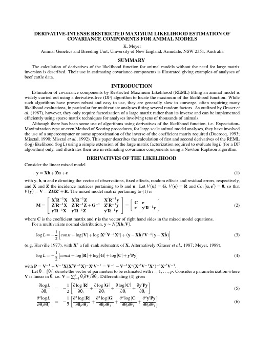
Restricted Maximum Likelihood to estimate variance components for animal models with severa
SUMMARY
The calculation of derivatives of the likelihood function for animal models without the need for large matrix inversion is described. Their use in estimating covariance components is illustrated giving examples of analyses of beef cattle data.
M −1 k=1
∑ log lkk
(7)
with M denoting the size of M, and noting that y Py = |M|/|C| (Smith, 1993)
2 y Py = lMM
(8)
Smith (1993) describes a general algorithm which allows the derivatives of the Cholesky factor of a matrix to be evaluated while carrying out the factorization, provided the derivatives of the original matrix are specified. Differentiating (7) and (8) then gives the derivatives of log |C| and y Py as simple functions of the diagonal elements of the Cholesky matrix and its derivatives.
maximum likelihood method

maximum likelihood method最大似然估计法(MaximumLikelihoodMethod,MLM)是一种常用的统计方法,它可以用于估计一个随机变量的参数。
在实际应用中,MLM被广泛应用于概率分布的参数估计、机器学习、数据挖掘等领域,具有很高的实用价值和广泛的应用前景。
一、最大似然估计法的基本概念最大似然估计法是一种基于概率统计的方法,它的核心思想是:在已知一些观测数据的情况下,估计这些数据所属的概率分布的参数,使得这些数据出现的概率最大。
这里的“概率最大”指的是在给定数据的条件下,所估计的参数能够使得这些数据出现的概率最大,也就是估计出的概率分布与观测数据的分布最为接近。
在数学上,最大似然估计法可以用极大化似然函数的方法来实现。
似然函数是指在已知参数的情况下,观测数据出现的概率分布。
具体地说,假设我们有一组观测数据{x1,x2,...,xn},它们来自某个概率分布,我们要估计这个概率分布的参数θ。
如果假设这个概率分布是一个已知的函数f(x;θ),那么似然函数可以表示为:L(θ|x1,x2,...,xn) = f(x1;θ)×f(x2;θ)×...×f(xn;θ) 这个似然函数的意义是,在已知参数θ的情况下,观测数据{x1,x2,...,xn}出现的概率。
我们的目标是找到一个最优的θ,使得这个似然函数最大化。
也就是说,最大化似然函数可以得到最优的参数估计。
二、最大似然估计法的实现步骤最大似然估计法的实现步骤可以分为以下几个步骤:1. 确定概率分布的形式:首先需要确定所要估计的概率分布的形式,比如正态分布、泊松分布、伽马分布等等。
这个选择需要根据实际问题来进行,一般可以根据数据的特点和分布情况来进行选择。
2. 写出似然函数:在确定了概率分布的形式之后,需要根据这个概率分布的密度函数写出似然函数。
这个似然函数的形式应该与上面提到的公式相同。
3. 求解似然函数的最大值:最大似然估计法的核心是求解似然函数的最大值。
Maximum Likelihood Estimators
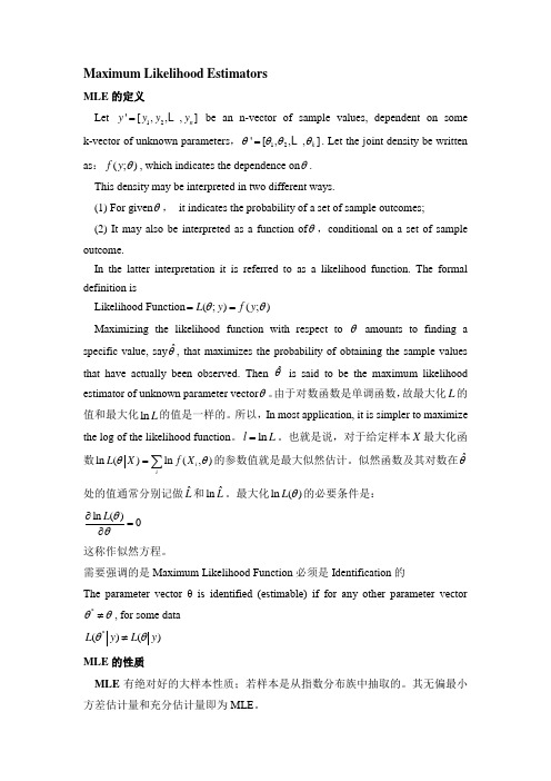
Maximum Likelihood EstimatorsMLE 的定义Let 12'[,,,]n y y y y = be an n-vector of sample values, dependent on some k-vector of unknown parameters ,12'[,,,]k θθθθ= . Let the joint density be written as :(;)f y θ, which indicates the dependence on θ. This density may be interpreted in two different ways.(1) For given θ, it indicates the probability of a set of sample outcomes; (2) It may also be interpreted as a function of θ,conditional on a set of sample outcome.In the latter interpretation it is referred to as a likelihood function. The formal definition isLikelihood Function (;)(;)L y f y θθ==Maximizing the likelihood function with respect to θ amounts to finding a specific value, say ˆθ, that maximizes the probability of obtaining the sample values that have actually been observed. Then ˆθ is said to be the maximum likelihood estimator of unknown parameter vector θ。
Maximum Likelihood Decoding of M-ary Orthogonal Modulated Signals for Multi-Carrier Spread-
Multi-Carrier Spread-Spectrum SystemsArmin Dekorsy,Stephan Fischer,and Karl-Dirk KammeyerUniversity of Bremen,FB-1,Department of TelecommunicationsP.O.Box330440,D-28334Bremen,Germany,Fax:+(49)-421/218-3341,e-mail:dekorsy@comm.uni-bremen.deABSTRACTFor a multi-carrier spread-spectrum(MC-SS)system,the innerspreading can be optimized by applying-ary orthogonal mod-ulation.In this paper,we investigate the concatenation of max-imum likelihood(ML)Viterbi decoding with-ary orthogonaldemodulation in a MC-SS system.The system operates over afrequency-selective Rayleigh fading indoor channel in the up-link.Wefirst evaluate the bit specific log-likelihood ratio for MLViterbi decoding and present an estimation of the ratio exploitingthe MC technique.Furthermore,the trade-off between channelcoding,-ary orthogonal modulation and simple spreading willbe considered by Monte-Carlo simulations.The results are al-ways compared with BPSK performance and they emphasize forthe concerned indoor transmission scenario that a moderate bit-error-rate can only be achieved if-ary orthogonal modulationis employed.All simulations are related to the European Hiperlan/2standard-ization whereas the results are generally valid.I.INTRODUCTIONFuture wireless radio systems need to make efficient use of thefrequency spectrum.One technique offering high spectrum effi-ciency is the multi-carrier-modulation technique orthogonal fre-quency division multiplexing(OFDM).With OFDM,the fadingof each subcarrier can be assumed as frequency-nonselective.Toachieve frequency diversity,OFDM can be combined with codedivision multiple access(CDMA),where the signal is spread overall subcarriers.This concept wasfirst introduced as OFDM-CDMA or also as multi-carrier(MC-)CDMA by[1,2]and isalso called MC-spread spectrum(MC-SS).In the recent few years,most publications dealing with MC-SShave been focused on classical modulation schemes such as BPSK[3,4]and several maximum likelihood(ML)decoding strategieswere proposed[5,6].Instead of using classical modulation schemes,SS techniquesoffer the possibility to apply-ary orthogonal modulation[7].With this modulation,the inner spreading of the MC-SS systemis optimized by spreading in two successive steps:(i)spreadingby the modulation itself and(ii)additional simple replication ofthe transmitted information into parallel subcarriers to performSS technique.The optimization is carried out without changingthe required bandwidth.Investigations without forward errorFigure1:MC-SS transmitter MC-SS transmitter(mobile station)with channel encoding andWalsh modulation is illustrated infig.1.For simplicity,one ofactive users is shown and subscripts are omitted.The data bits,each of duration,are convolution-ally encoded with code rate.The input of the en-coder is a sequence of subsequent data bits and the out-put is the encoded bit sequence of bits,each with duration .After block interleaving()the encoded bits are serial/parallel converted to groups of bits each.The Walsh modulation maps the encoded bits to one corre-sponding Walsh symbol(vector),including Walsh chips.Each of the parallel Walsh chips has a duration of.This modulation can also be interpreted as a block code of rate.The set of or-thogonal Walsh symbols describes the Hadamard-Matrix [7,10],and the Euclidian distance is identical for all possible pairs of symbols and equals(1)To obtain the transmitted symbols,the Walsh chips are repli-cated into parallel copies where each branch of the parallel stream is multiplied with one chip of the user specific PN-code(3) Thefirst term of(3)describes the spreading of the Walsh mod-ulation,the second one the ratio of simple spreading()over the code rate of the channel code,whereas the third term takes into account the guard time.For our comparisons,the product remains unchanged due to the exploitation of the inherently overall spreading factor1.Decreasing the BER can be achieved by sharing between channel coding,-ary orthogonal Walsh modulation and simple spreading.The data rate is based on binary modulation without channel coding()and the bandwidth is generally given.B.Coherent receiverThe MC-SS receiver for-ary orthogonal Walsh modulation is shown infig.2.Paying attention to active users,the received signal after OFDM demodulation and deinterleaving()can be written as a sum of vectors(4) with elements and.The vector represents Additive White Gaussian Noise AWGN.After multiplication with the user spe-cific code and equalization,thefirst part of despreading is ob-tained by subcorrelating subcarriers.Reception for the user is assumed(subscripts are omitted).The components of are given by(5) where indicates the equalization coefficient of the-th subcar-rier.We take into account the well-known equalization scheme maximum ratio combining(MRC)which shows the best perfor-mance for an uplink transmission[8].If perfectly known channel coefficients are assumed2,then.To enable maximumFigure2:MC-SS receiver likelihood detection(MLD),the signal is correlated with all pos-sible Walsh symbols,.The MLD canbe realized by the Fast Hadamard Transform(FHT),where theoutput vector contains decision variables.In case of MLD,optimum decoding,e.g.of a convolutional code,is performedby the application of a soft input Viterbi algorithm(V A)wherechannel state information is exploited.Therefore,the reliabil-ity estimator exploits the decision variables to calculate theassigned bit specific log-likelihood ratio which is fed to theViterbi channel decoder after deinterleaving().Afterwards,we obtain the estimated data stream with bits.III.ML DECISION DECODINGIn the following,we will derive the bit specific log-likelihoodcriterion for ML decoding of-ary orthogonally modulated sig-nals.We consider coherent MC-SS demodulation with MRC equalization.The MAI is taken into account as AWGN and inde-pendent adjacent fading subcarriers ensured by perfect frequency interleaving()are assumed.A.Antipodal TransmissionLet usfirst assume binary antipodal transmission on a single car-rier system with denoting the-th transmitted en-coded bit.Hard decision at the receiver leads to the binary en-coded bit.For a memoryless discrete binary sym-metric channel the likelihood criterion for ML channel decodingis given by[12]of the log-likelihood ratio can be interpretedas a reliability indicator for the hard decided code bit.Due to the fact that involves channel state information the application of eq.(6)results in optimum performance under time-variant channels.For example,if the transmitted signal suffers from fading and is disturbed by AWGN,the log-likelihood ratio results in(8) If equiprobable transmitted symbols are assumed,we get .Due to the statistical independence of the com-ponents of,the conditional probability density can be(9)where and.The terms and can be calculated uniquely.In case of the considered coherent MRC detection one obtain a zero mean Gaussian distribution with variance for the-th component where the hypothesis does not hold,i.e.:exp(11) with mean(13)(the union of all elementary events has probability one).The calculation of(14)requires the knowledge of the noise variance and the expected value of the average channel energy over all subcarriers. These parameters can be estimated as follows:(i)noise variance estimationAssuming that the decision variable with maximum magnitude, denoted by,represents the true hypothesis,we obviously obtain an estimate of the noise power by the mean over components containing the false hypotheses:(16) With(13)-(16),all parameters needed for the calculation of the conditional symbol probability(12)are known.The results can be summarized for all hypotheses:If the symbols are re-placed by their corresponding bit patternsin antipodal representation,we obtain(e.g.for)...(17)The application of eq.(6)requires knowledge of the probabilities of individual bit-decisions which can be gained by a columnwise evaluation of(17).Note,atfirst,that eq.(6)does not depend on the specific choice of the decision for bit,sinceand serves as a soft input for the Viterbi channel decoder.The other bits are treated equivalently.IV.SYSTEM COMPARISONA.System descriptionRelated to the European H IPERLAN/2standardization,the results followed are given for a transmission over an indoor Rayleigh fading channel.The bandwidth is in the range.A velocity of m/s results in a very low maximum Doppler frequency of about.Hence,long symbol-ary orthogonal modulation can be applied.Furthermore,due to the very low maximum Doppler frequency,the fading on each subcarrier is highly statistically dependent.To avoid bursty er-rors,sufficient frequency interleaving ()is required.First,the indoor channel is modeled assuming sufficient frequency inter-leaving.Subsequently,we take into account an exponential delayprofile with a maximum delay spread ofns and a coherent bandwidth of approximately .I.e.the number of independent subcarriers is reduced dramatically.The trade-off between coding and spreading is carried out for anunchanged product(3)and is based on binary modulation without FEC withsubcarriers.The guard time is chosen to be ns.This system design results in a data rate of kbit/s for all cases of spreading and coding.A block interleaver ()with rows and columns is used to separate the channel code and the -ary Walsh modulation.We employed two convolutional codes of rate and,both with constraint length [10].For all cases,active users are taken into account and perfect channel estimation as well as perfect synchronization is assumed for the considered user.B.Simulation ResultsFig.4shows the BER of the -ary Walsh modulation forby sharing between simple spreading andFEC of rates ;see (3).Independent of the -ary modulation the results indicate that choosing a higher amount of simple spreading combined with less powerful FEC ()outperforms the scheme with lower amountcombined with more powerful FEC ().Note the gain of approximately in at a BER of for the -ary modulation.This fact can be explained for by1010101010B E R →Figure coding,-ary Walsh modulation and simple spreading forand codes of ratethe higher loss due to an unchanged guard time but a shorter symbol duration and an additional lower energy of the coded bit in front of the Viterbi decoder 4.Moreover,less number ofsion over an indoor channel with coherence bandwidth of ap-proximately.BPSK and-ary Walsh modulation are considered.In contrast tofig.5,there exists a significant loss due to the statistical dependence of the adjacent subcarriers.The re-sults emphasize for an MC-SS uplink transmission over an indoor Rayleigh fading channel that BPSK even combined with FEC leads to an unacceptable BER.Moderate performance can only be achieved if-ary orthogonal Walsh modulation is applied. One has to mention that the degradation is mainly caused by the insufficient frequency interleaving.There exists only a slight degradation due to the assumption of independent subcarriers for the derivations of the log-likelihood ratios.V.CONCLUSIONIn this paper,we have investigated the concatenation of-ary orthogonal Walsh modulation and ML Viterbi decoding for the MC-SS transmission over a frequency-selective slowly Rayleigh fading channel in the uplink.In particular,we havefirst evalu-ated the bit specific log-likelihood ratio of the-ary orthogonal modulated signal for the ML Viterbi decoding.Assuming an un-changed bandwidth and data rate,we further analyzed the trade-off between coding and spreading to optimize the BER.Monte-Carlo simulation results indicate to better strengthen the inner spreading consisting of-ary orthogonal modulation and simple spreading with an inherently less powerful channel code.The results are always compared with BPSK performance and it is shown that already-ary orthogonal Walsh modulation outper-forms BPSK.Moreover,they emphasize that for an indoor sce-nario a moderate BER can only be achieved if the inner spreading is optimized,for example,by applying-ary orthogonal Walsh modulation.BPSK even combined with channel coding leads to an unacceptable BER.REFERENCES[1]K.Fazel and L.Papke.On the performance of convolutionally-coded CDMA/OFDM for mobile radio communication system.In Proc.IEEE Int.Symp.on Personal,Indoor and Mobile Radio Commun.(PIMRC’93),pages D3.2.1–D3.2.5,September1993. [2]N.Yee,J.-P.Linnartz,and G.Fettweis.Multi-Carrier CDMA inIndoor Wireless Radio Networks.In Proc.IEEE Int.Symp.on Personal,Indoor and Mobile Radio Commun.(PIMRC’93),pages D1.3.1–D1.3.5,September1993.[3]S.Kaiser.On the Performance of Different Detection Techniquesfor OFDM-CDMA in Fading Channels.In Proc.IEEE Global Telecommunication Conference(GLOBECOM’95),pages2059–2063,Singapore,November13–171995.[4]R.Prasad and S.Hara.An Overview of Multi-Carrier CDMA.InProc.IEEE Fourth Int.Symposium on Spread Spectrum Techniques &Applications(ISSSTA’96),volume1,pages107–114,Mainz, Germany,September22–251996.[5]S.Kaiser and L.Papke.Optimal Detection when CombiningOFDM-CDMA with Convolutional and Turbo Channel Coding.In Proc.IEEE International Conference on Communications (ICC’96),pages343–348,Dallas,June23–271996.[6]R.A.Stirling-Gallacher and G.J.R.Povey.Different ChannelCoding Strategies for OFDM-CDMA.In Proc.IEEE Veh.Tech.71997.[7] A.J.Viterbi.CDMA–Principles of Spread Spectrum Communica-tion.Addison–Wesley,1995.[8] A.Dekorsy and K.D.Kammeyer.M-ary Orthogonal Modulationfor MC-CDMA Systems in Indoor Wireless Radio Networks.InG.P.Fettweis and K.Fazel,editors,First International Workshopon MC-SS,volume1,pages69–76,Oberpfaffenhofen,Germany, April1997.Kluwer Academic,ISBN0-7923-9973-0.[9]M.Benthin and K.D.Kammeyer.Viterbi Decoding of Convo-lutional Codes with Reliability Information for a Noncoherent RAKE-Receiver in a CDMA-Environment.In IEEE Global Telecommunications Conference(GLOBECOM),pages1758–1762,San Francisco,November28–December21994.[10]J.G.Proakis.Digital Communications.McGraw–Hill,thirdedition,1995.[11] A.Dekorsy and K.D.Kammeyer.M-ary Orthogonal Modulationfor Multi-Carrier Spread-Spectrum Uplink Transmission.Ac-cepted for Proc.IEEE International Conference on Communica-tions(ICC’98),Atlanta,June7–11,1998.[12]J.Hagenauer.Viterbi Decoding of Convolutional Codes forFading-and Burst–Channels.In Proc.of the1980Zurich Seminar on Digital Communications,volume IEEE Catalog No.80CH1521–4COM,pages G2.1–G2.7,1980.[13]S.Kaiser.Trade–off between Channel Coding and Spreadingin Multi-Carrier CDMA Systems.In Proc.IEEE Fourth Int.Symposium on Spread Spectrum Techniques&Applications (ISSSTA’96),volume3,pages1366–1370,Mainz,Germany, September22–251996.。
maximum likelihood estimation method -回复
maximum likelihood estimation method -回复什么是最大似然估计方法(Maximum Likelihood Estimation Method)?最大似然估计方法是一种用于估计统计模型中的参数的方法。
它基于一个假设,即给定了一些观测数据,我们想要找到一个参数的值,使得这些数据出现的概率最大。
换句话说,最大似然估计方法尝试找到“最有可能”解释观测数据的参数值。
最大似然估计方法的步骤:1. 确定概率分布函数:首先,我们需要确定观测数据所遵循的概率分布函数。
这个函数的选择通常基于对数据的初步分析和领域知识。
例如,如果我们的数据符合正态分布,则我们可以选择正态分布函数作为概率分布函数。
2. 构建似然函数:似然函数是给定观测数据的条件下,参数取不同值时观测数据发生的概率的函数。
它是参数的函数,而观测数据是固定的。
似然函数可以通过将观测数据的概率密度函数乘起来得到。
假设我们有n个独立观测数据,那么似然函数可以表示为L(θX₁, X₂, ..., Xₙ),其中θ表示参数,X₁, X₂, ..., Xₙ表示观测数据。
3. 最大化似然函数:为了找到使观测数据出现的概率最大的参数值,我们需要最大化似然函数。
这可以通过计算似然函数对参数的导数,然后将导数等于零求解得到。
为简化计算,通常会对似然函数取对数,得到对数似然函数。
因为对数函数是单调递增的,所以最大化对数似然函数等价于最大化似然函数本身。
4. 估计参数值:在最大化似然函数的过程中,我们找到了使观测数据概率最大的参数值,这就是我们的估计值。
这个估计值代表了我们对参数的最优猜测。
它可以用来描述数据分布,进行统计推断和预测等。
最大似然估计方法的优点:- 直观易懂:最大似然估计方法直观易懂,基于概率的思想,非常符合人们的直觉。
- 一致性:当样本量趋于无穷大时,最大似然估计方法通常能够收敛于真实参数值,具有一致性的性质。
- 有效性:在满足一定条件下,最大似然估计方法可以得到渐进有效的估计量,即估计量的均方差收敛于费舍尔信息。
最大似然估计的关键公式概览

最大似然估计的关键公式概览最大似然估计(Maximum Likelihood Estimation,简称MLE)是统计学中一种常用的参数估计方法,它通过寻找最大化样本观测值在给定参数下的概率,从而得到最优的参数估计值。
在实际应用中,最大似然估计被广泛应用于各个领域,例如机器学习、统计分析、金融风险评估等。
本文将对最大似然估计中的关键公式进行概览,帮助读者更好地理解和应用该方法。
1. 似然函数(Likelihood Function)在最大似然估计中,首先需要定义似然函数。
似然函数是一个关于参数的函数,表示在给定参数的条件下,样本观测值出现的可能性。
在统计学中,常用L(θ;x)表示似然函数,其中θ表示参数,x表示样本观测值。
似然函数的计算通常基于样本观测值的分布假设,例如正态分布、泊松分布等。
2. 对数似然函数(Log-Likelihood Function)为了方便计算和优化,通常将似然函数取对数得到对数似然函数。
对数似然函数的形式为ln L(θ;x),其中ln表示自然对数。
对数似然函数的计算可以将乘法转化为加法,简化计算过程。
同时,对数函数的单调性保证了最大化似然函数和最大化对数似然函数有相同的结果。
3. 最大似然估计的目标函数最大似然估计的目标是找到合适的参数值,使得似然函数或对数似然函数达到最大值。
因此,需要构建一个目标函数,以参数为变量,似然函数或对数似然函数为目标,通过优化算法求解最优的参数估计。
对于似然函数而言,目标函数为:argmax L(θ;x)对于对数似然函数而言,目标函数为:argmax ln L(θ;x)其中argmax表示使目标函数达到最大值的参数取值。
4. 最大化目标函数的方法为了求解使目标函数最大化的参数取值,通常使用数值优化方法。
常见的方法有梯度下降法、牛顿法、拟牛顿法等。
梯度下降法是一种基于函数梯度信息的迭代优化算法,通过计算目标函数关于参数的梯度方向,并不断朝着梯度下降的方向更新参数值,直至达到最优解。
面向GF-2遥感影像的U-Net城市绿地分类
700E-mail:***********.cn Website: Tel: ************©中国图象图形学报版权所有中国图象图形学报JO U R N A L O F IM A G E A ND G R A P H IC S中图法分类号:TF79 文献标识码:A 文章编号:1006-8961(2021)03-0700-14论文引用格式:Xu Z Y, Zhou Y,Wang S X ,Wang L T and Wang Z Q. 2021. U-Net for ur 丨)an green space classification in Gaofen-2 remote sensing images. Jmimal oflmage and GraPhiC S ,26(03) :0700-07丨3(徐知宇,周艺,王世新,王丽涛,王振庆.2021.面向GF-2遥感影像的U-Net 城市绿地分类.中国图象图形学报,26(03) :0700-0713) [ D01:10. 1 丨 834/j i g . 200052 ]面向GF -2遥感影像的U_Net 城市绿地分类徐知宇匕2,周艺、王世新\王丽涛、王振庆h 2I .中国科学院空天信息创新研究院,北京100094 ; 2.中国科学院大学,北京100049摘要:目的高分2号卫星(G F-2)是首颗民用高空间分辨率光学卫星,具有亚米级高空间分辨率与宽覆盖结合 的显著特点,为城市绿地信息提取等多领域提供了重要的数据支撑。
本文利用G F-2卫星多光谱遥感影像,将一种 改进的U-Net 卷积神经网络首次应用于城市绿地分类,提出一种面向高分遥感影像的城市绿地自动分类提取技 术。
方法先针对小样本训练集容易产生的过拟合问题对U-Net 网络进行改进,添加批标准化(batch normalization , BN) 和 dropout 层获得 U-Net + 模型; 再采用随机裁剪和随机数据增强的方式扩充数据集, 使得在充分利用影像 信息的同时保证样本随机性,增强模型稳定性。
Maximum Likelihood Estimation
It is tempting to view the likelihood function as a probability density for θ, and to think of l ( θ | x) as the conditional density of θ given x. This approach to parameter estimation is called ducial inference, and is not accepted by most statisticians. One potential problem, for example, is that in many cases l ( θ | x) is not integrable ( l ( θ | x) dθ → ∞) and thus cannot be normalized. A more fundamental problem is that θ is viewed as a xed quantity, as opposed to random. Thus, it doesn't make sense to talk about its density. For the likelihood to be properly thought of as a density, a Bayesian approach is required.
/content/m11446/1.5/
Connexions module: m11446
3
While the likelihood principle itself is a fairly reasonable assumption, it can also be derived from two somewhat more intuitive assumptions known as the suciency principle and the conditionality principle. See Casella and Berger, Chapter 6 [1].
- 1、下载文档前请自行甄别文档内容的完整性,平台不提供额外的编辑、内容补充、找答案等附加服务。
- 2、"仅部分预览"的文档,不可在线预览部分如存在完整性等问题,可反馈申请退款(可完整预览的文档不适用该条件!)。
- 3、如文档侵犯您的权益,请联系客服反馈,我们会尽快为您处理(人工客服工作时间:9:00-18:30)。
Vol. 51, No. 4 (July. 1983)
SOLUTION AND MAXIMUM LIKELIHOOD ESTIMATION OF DYNAMIC NONLINEAR RATIONAL EXPECTATIONS MODELS BY RAY C. FAIR AND JOHN B. TAYLOR’ A s0Iulim method and an esrimation method for nmlinear mimal expectations models are presented in thin paper. The solution method can be used in forecasting and
mean zero and which may be correlated across equations (Eui,uj, f 0 for i #j) and wer time (Eu,,u, i 0 for t # s). The model is nonlinear in that the functionf, may be nonlinear in the variables, parameters, and expectations, although we will require certain regularity conditions on these functions and their derivatives with respect to yI and ai. It is a r&ma/ expecratiom model in that expectations of future endogenous variables are conditional forecasts based on the model itself, and it is dynamic in ~that the lags and expected leads of the endogenous variables appear in the equatimx2 The main objectives of this paper are to describe and
1. INTRODUCTION
CONSIDER THE DYNAMIC RATIONAL expectations
model given by
(i=
11...,
n),
where y( is an n-dimensional vector of endogenous variables at time r, n, is a vector of exogenous variables at time I, E,_, is the conditional expectations
operator vector based on the model and on information of parameters, and uj, is a stationary scalar through random period f1, ai is a which has variable
‘ The research described in this paper was financed by Grants SOC77-03274 and SE.79.26724 from the National Science Foundation. The authors are indebted to .A& Dagli for computaional assistance. ‘ Several properties of the general form represented in model (1 j should be noted. By appropriate conswuction. the model ran include expeclo~ions of nonlinear *unctions of the endogenaus variables. of Et_, yli in one of the equations indicates that the For example. if ,vir = yb, then the appearance agents are concerned with the conditionally expected variance of y,,. Also, the model permits nonlinear restrictions on the a, paramews both within and across equations. However, the model does Dot explioitly include expectations based on current period (f) inform&x. The i*coqxneion of such variables does not cause difficulties far the solution of the model (as we describe below), but it does cause difficulties for estimation since the Jacobian of the transformatian from the us to they, is altered.
1170
R. C. FAIR
ቤተ መጻሕፍቲ ባይዱ
AND
J. R. TAYLOR
investigate numerically (i) a method for solving the model for the vector ,v~ in terms of its past values and the values of the exogenous variables x, and (ii) a method for obtaining the maximum likelihood estimates of the parameters a, and the covariance structure of the ui, given a series of observations on y, and x,, 1=1,...,T. The solution method is an extension of the iterative technique used in Fair [3]. In addition to dealing with serial correlation and multiple viewpoint dates, the extension involves an iterative procedure (called Type III in the following discussion) designed to insure numerical convergence to the rational expectations solution. The estimation method is an extension to the nonlinear case of full information maximum likelihood techniques designed for linear rational expectations models, as described by Wallis [15] and Hansen and Sargent [7, 81.’ Applications to particular economic problems are found in Sargent 1121 and Taylor [14]. Full information estimation techniques are particularly useful for rational expectations models because of the importance of cross equations restrictions, where most of the testable implications of the rational expectations hypothesis lie. For linear models one can explicitly calculate a reduced form of model (l), in which the expectations variables are eliminated and nonlinear restrictions are placed on the parameters. Under the assumption that the ui, are normally distributed this restricted reduced form can be used to evaluate the likelihood function in terms of the structural parameters. The maximum of the likelihood function with respect to the structural parameters is found using numerical nonlinear tnaximization routines. For nonlinear models the reduced form cannot be calculated explicitly, but it can be calculated numerically. Our estimation strategy is to replace the calculation of the restricted reduced form in linear models with the numerical solution in nonlinear models. This permits one to evaluate the likelihood function in terms of the unknown structural parameters, much like in the linear case. While we feel that the nonlinear methods described will expand the range of empirical problems that can be approached using rational expectations, there is a limitation that may affect their general applicability. Because of computational costs it is necessary in some applications to approximate the conditional expectations that appear in (1) by setting the future disturbances u,, equal to their conditional means in a deterministic simulation of the model. In nonlinear rational expectations models the conditional expectations will involve higher order moments of the I+, in addition to their means. (See Lucas and Prescott [lo], for example.) As we describe in the paper, it is possible to use stochastic