Exact solution of Schrodinger equation for modified Kratzer's molecular potential with the
类氦离子schrodinger方程直接求解的精确势谐方法

类氦离子schrodinger方程直接求解的精确势谐方法类氦离子是由两个电子和一个氦核组成的三体系统,其精确解析解是无法求得的。
然而,通过使用精确势谐方法,我们可以得到类氦离子的近似解。
精确势谐方法是一种基于势能函数的展开式的方法,它将势能函数展开为一组谐函数的线性组合。
在类氦离子的情况下,我们可以将势能函数表示为:V(r1,r2) = -2/r1 - 2/r2 + 1/r12其中,r1和r2是两个电子与氦核之间的距离,r12是两个电子之间的距离。
通过将势能函数展开为谐函数的线性组合,我们可以得到类氦离子的Schrodinger方程的精确解。
具体来说,我们可以将Schrodinger方程表示为:HΨ = EΨ其中,H是哈密顿算符,Ψ是波函数,E是能量。
通过将波函数表示为一组谐函数的线性组合,我们可以得到:Ψ(r1,r2) = ΣCnmψnm(r1,r2)其中,Cnm是系数,ψnm是谐函数。
将波函数代入Schrodinger方程,我们可以得到:ΣCnm(Hψnm) = EΣCnmψnm通过将哈密顿算符表示为谐函数的线性组合,我们可以得到:Hψnm = Enmψnm其中,Enm是能量。
将能量代入Schrodinger方程,我们可以得到:ΣCnmEnmψnm = EΣCnmψnm这是一个矩阵方程,我们可以通过对矩阵进行对角化来求解能量和系数。
通过这种方法,我们可以得到类氦离子的精确解。
总之,精确势谐方法是一种有效的求解类氦离子Schrodinger方程的方法。
通过将势能函数展开为谐函数的线性组合,我们可以得到精确解。
虽然这种方法需要计算大量的系数,但是它可以提供非常精确的结果。
因此,它在量子化学中得到了广泛的应用。
Complete solution of the Schrodinger equation for the time-dependent linear potential

Consider the Schr¨odinger equation for a particle with time-dependent mass moving in a time-dependent linear potential, which can be described by the Schr¨odinger equation in the unit of h¯ = 1,
The purpose of the present paper is to undertake a completely analytical solution for the problem above along the idea in [15,16] by means of a simple algebra, named ’time-space transformation method’ [17]. With the timespace transformation method, in [17], we transformed the Schr¨odinger equation with TDHO into that with time independent harmonic oscillator. But here we will try to transform a Schr¨odinger equation with time-dependent linear potential into that of a free particle. According to [15,16], there are only two solutions with nonspreading properties for the quantum treatment of a free particle. One solution is based on the wave function of the plane wave, and the other is with the form of the Airy function. However, as far as we know, no one has reported these two solutions simultaneously in treating the Hamiltonian with time-dependent linear potential. Therefore, in what follows, we will consider a more general case than in Ref.[14,15], i.e., a particle with time-dependent mass moving in the time-dependent linear potential. It can be found that the solution in Ref.[14] is merely a particular case for
用动力系统方法研究一类时间分数阶扩散方程的精确解

Advances in Applied Mathematics 应用数学进展, 2023, 12(6), 2896-2903 Published Online June 2023 in Hans. https:///journal/aam https:///10.12677/aam.2023.126291用动力系统方法研究一类时间分数阶扩散方程的精确解黎超玲重庆师范大学数学科学学院,重庆收稿日期:2023年5月25日;录用日期:2023年6月19日;发布日期:2023年6月27日摘要随着时代的发展,分数阶微分模型的应用越来越广泛,故对其研究非常有必要。
本文在Riemann-Liouville 分数阶导数的定义下利用半固定式变量分离法与动力系统理论相结合的方法,研究了一类时间分数阶扩散方程的精确解,获得了方程的一系列精确解,通过解的坐标演化图直观地展示了在不同参数条件下的扩散现象。
关键词时间分数阶扩散方程,Riemann-Liouville 分数阶导数,半固定式变量分离法,动力系统方法,精确解Exact Solutions of a Class of Time-Fractional Diffusion Equation by Dynamic System MethodChaoling LiSchool of Mathematical Sciences, Chongqing Normal University, ChongqingReceived: May 25th , 2023; accepted: Jun. 19th , 2023; published: Jun. 27th , 2023AbstractWith the development of the times, the application of fractional differential model is more and more extensive, so it is very necessary to study it. In this paper, under the definition of Riemann-Liouville fractional derivative, the exact solution of a class of time fractional diffusion equations is studied by combining semi-fixed variable separation method with dynamic system theory, and a series of exact solutions of the equations are obtained. The diffusion phenomenon under different parameter con-ditions is intuitively displayed through the coordinate evolution diagram of the solutions.黎超玲KeywordsTime Fractional Diffusion Equation, Riemann-Liouville Fractional Derivative, Semi-Fixed Variable Separation Method, Dynamical System Method, Exact SolutionsCopyright © 2023 by author(s) and Hans Publishers Inc.This work is licensed under the Creative Commons Attribution International License (CC BY 4.0)./licenses/by/4.0/1. 引言分数阶微积分和整数阶微积分都起源于同一个时代,即Leibniz 时代。
张永德教授量子力学讲义 第十一章

第三部分 开放体系问题第十一章含时问题与量子跃迁本章讨论量子力学中的时间相关现象。
它们包括:含时问题求解的一般讨论、含时微扰论、量子跃迁也即辐射的发射和吸收问题。
如果说,以前各章主要研究量子力学中的稳态问题,本章则专门讨论非稳态问题。
根据第五章中有关叙述,由于我们所处时空结构的时间轴固有的均匀性,孤立量子体系的Hamilton量必定不显含时间,从而遵守不显含时间的Schrödinger方程。
因此,这里含时Schrödinger方程所表述的量子体系必定不是孤立的量子体系,而是某个更大的可以看作孤立系的一部分,是这个孤立系的一个子体系。
当这个子体系和孤立系的其他部分存在着能量、动量、角动量、甚至电荷或粒子的交换时,便导致针对这个子体系的各类含时问题。
在了解本章(以及下一章)内容的时候,有时需要注意这一点。
§11.1 含时Schrödinger方程求解的一般讨论1, 时间相关问题的一般分析量子力学中,时间相关问题可以分为两类:i, 体系的Hamilton量不依赖于时间。
这时,要么是散射或行进问题,要么是初始条件或边界条件的变化使问题成为与时间相关的现象。
“行进问题”例如,中子以一定的自旋取向进入一均匀磁场并穿出,这是一个自旋沿磁场方向进动的时间相关问题;258259“初始条件问题”比如,波包的自由演化,这是一个与时间相关的波包弥散问题。
更一般地说,初态引起的含时问题可以表述为:由于Hamilton 量中的某种相互作用导致体系初态的不稳定。
例如Hamilton 量中的弱相互作用导致初态粒子的β衰变等;最后,“边界条件变动”也能使问题成为一个与时间相关的现象。
例如阱壁位置随时间变动或振荡的势阱问题等。
ii, 体系的Hamilton 量依赖于时间。
这比如,频率调制的谐振子问题或是时间相关受迫谐振子问题,交变外电磁场下原子中电子的状态跃迁问题等等。
如果问题允许有精确的、解析的解,就称相应的Hamilton 量H 为可积的,相应系统为可积体系。
带非定域项schrodinger方程的jost解

带非定域项schrodinger方程的jost解在量子力学中,Schrödinger方程是研究量子系统的一个常用方程。
对于一维系统,Schrödinger方程可以写成如下形式:\[H\psi(x) = E\psi(x)\]其中H是系统的哈密顿算符,ψ(x)是波函数,E是能量。
通常情况下,Schrödinger方程是一个定域的方程,即和位置x有关系的项是局部的。
然而,在一些情况下,Schrödinger方程可以包含非定域项,即和位置x有关系的项是非局部的。
这种情况下的Schrödinger方程被称为带非定域项的Schrödinger方程。
\[H\psi(x) = E\psi(x) + V(x)F[\psi](x)\]其中V(x)是定域势能项,F[\psi](x)是非定域项,可能包含了波函数ψ在整个空间上的积分或导数等。
在研究带非定域项的Schrödinger方程时,一个重要的概念是Jost 解。
Jost解是一种特殊的解,它们具有一些特殊的性质。
Jost解可以通过一个无穷级数的形式来表示:\[\psi(x) = \sum_{n=0}^{\infty}a_ne^{ikx}\]其中k是一个实数,a_n是系数。
对于带非定域项的Schrödinger方程,Jost解可以写成如下形式:\[\psi(x) = \sum_{n=0}^{\infty}a_ne^{ikx} + \int dkF[k]\phi(k)e^{ikx}\]其中F[k]是一个与波矢k相关的函数,用来描述非定域项的影响。
φ(k)是一个与波矢k相关的函数,它是另外一个方程的特解,该方程不包含非定域项。
这个方程通常被称为约化方程。
Jost解的一个重要性质是它们满足正交归一条件。
即,Jost解的内积满足如下关系:\[\int dx \psi^*(x)\psi(x) = 1\]根据这个性质,可以推导出Jost解的系数a_n满足一组正交归一条件:\[\int dx \psi_n^*(x)\psi_m(x) = \delta_{nm}\]其中δ_nm是Kronecker delta符号,当n=m时为1,否则为0。
schordinger方程

薛定谔方程(Schrödinger equation),又称薛定谔波动方程(Schrodinger wave equation),是由奥地利物理学家薛定谔提出的量子力学中的一个基本方程,也是量子力学的一个基本假定。
它是将物质波的概念和波动方程相结合建立的二阶偏微分方程,可描述微观粒子的运动,每个微观系统都有一个相应的薛定谔方程式,通过解方程可得到波函数的具体形式以及对应的能量,从而了解微观系统的性质。
在量子力学中,粒子以概率的方式出现,具有不确定性,宏观尺度下失效可忽略不计。
Exact solution to the Schr{o}dinger equation for the quantum rigid body

There is huge degeneracy of the hyperspherical basis, and the matrix elements of the potential have to be calculated between different hyperspherical harmonic states [10], because the interaction in the three-body problem is not hyperspherically symmetric. The quantum rigid body (top) can be thought of as the simplest quantum three-body problem where the internal motion is frozen. To solve exactly the Schr¨ odinger equation for the rigid body is the first step for solving exactly the quantum three-body problems. Wigner first studied the exact solution for the quantum rigid body (see P.214 in [17]) from the group theory. He characterized the position of the rigid body by the three Euler angles α, β , γ of the rotation which brings the rigid body from its normal position into the position in question, and obtained the exact solution for the quantum rigid body, which is nothing but the Wigner D -function. For the quantum
Exact Solutions of the Time Dependent Schroedinger Equation in One Space Dimension
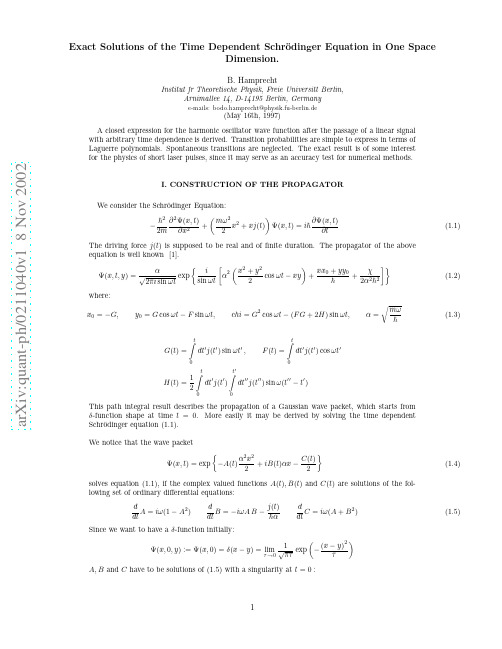
a r X i v :q u a n t -p h /0211040v 1 8 N o v 2002Exact Solutions of the Time Dependent Schr¨o dinger Equation in One SpaceDimension.B.HamprechtInstitut fr Theoretische Physik,Freie Universitt Berlin,Arnimallee 14,D-14195Berlin,Germanye-mails:bodo.hamprecht@physik.fu-berlin.de(May 16th,1997)A closed expression for the harmonic oscillator wave function after the passage of a linear signal with arbitrary time dependence is derived.Transition probabilities are simple to express in terms of Laguerre polynomials.Spontaneous transitions are neglected.The exact result is of some interest for the physics of short laser pulses,since it may serve as an accuracy test for numerical methods.I.CONSTRUCTION OF THE PROPAGATORWe consider the Schr¨o dinger Equation:− 2∂x 2+mω2∂t(1.1)The driving force j (t )is supposed to be real and of finite duration.The propagator of the above equation is well known [1].Ψ(x,t,y )=α2πi sin ωt exp i 2cos ωt −xy+xx 0+yy 02α2 2 (1.2)where:x 0=−G,y 0=G cos ωt −F sin ωt,chi =G 2cos ωt −(F G +2H )sin ωt,α=(1.3)G (t )=tdt ′j (t ′)sin ωt ′,F (t )=tdt ′j (t ′)cos ωt ′H (t )=12+iB (t )αx −C (t )dtA =iω(1−A 2)dαd√τA,B and C have to be solutions of (1.5)with a singularity at t =0:1A(t)=−i cotωtB(t)=−G(t)αsinωtC(t)=log(2πi sinωt)−iα2y2cotωt−i 2y+G +2i√2α2+i ωt m+1m!2−iH√√√2 (−ir∗)n|a n|2=R nα22 dy(3.1) The integral evaluates to:Ψ(x,t)=4 πexp −α2x 0=−i(F +iG )e −iωt2α2 2+1α2p =−(F cos ωt +G sin ωt )(3.3)IV.APPENDIXWe evaluate equation (2.1),using the generating function for the Hermite polynomials.If γm,n is the coefficient of w m z n in the Taylor expansion of:J =α∞−∞Ψ(x,t,y )e 2(wx +zy )α−w2−z 2−x 2+y2n !m !2γm,n (4.1)Now:J =12πi sin t∞ −∞exp −X T AX +2P T X −Q α2dX = 2i sin tdetAexp P T A −1P −Q(4.2)where:X =αxy P =w −iG2α(F −G cot ωt ) A =12cot ωti2sin ωt12cot ωtQ =w 2+z 2+iα2 2HWe find:det A =−ie iωtα−iwF +iG4α2 2(4.4)Therefore:a m,n =2n +mexp−F 2+G 2+4iHαm −k F −iGk !(m −k )!(n −k )!Extracting common factors from the sum and replacing k by m −k in the summation,we obtain:a n.m =√4α2 2 −i F −iG2α n −m m k =0−F 2+G 2k !(m −k )!(n −m +k )!The finite sum in this expression defines a Laguerre polynomial.Therefore:a n.m = n !exp −|r |2α22(−ir ∗)n −m L (n −m )m (|r |2)(4.5)3where:r=F+iG2α=12αtdt′j(t′)e iωt′which proves equation(2.2).。
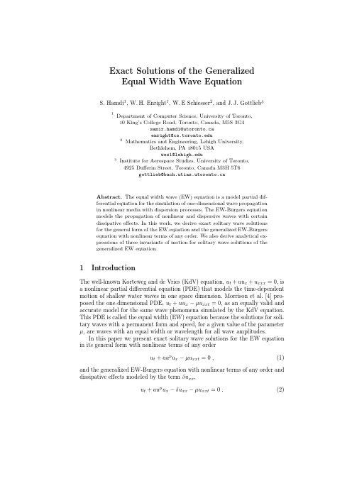
Exact Solutions of the Generalized Equal Width Wave Equation
(u )2 dξ = k2 , as ξ −→ +∞ ,
(13)
By substituting (14) into (13) and using the relation (11), we obtain the analytical expression of the following important square integral,
2
Derivation of the Exact Solutions
We concentrate on finding an exact solitary wave solution of the form u(x, t) = u(x − x0 − Ct) . (3)
This corresponds to a traveling-wave propagating with steady celerity C . We are interested in solutions depending only on the moving coordinate ξ = x − x0 − Ct as, u(x, t) = u(x − x0 − Ct) ≡ u(ξ ) . (4) Substituting into (2), the function u(ξ ) satisfies a third order nonlinear ordinary differential equation (ODE), −Cu + aup u − δu + µCu =0, (5)
Abstract. The equal width wave (EW) equation is a model partial differential equation for the simulation of one-dimensional wave propagation in nonlinear media with dispersion processes. The EW-Burgers equation models the propagation of nonlinear and dispersive waves with certain dissipative effects. In this work, we derive exact solitary wave solutions for the general form of the EW equation and the generalized EW-Burgers equation with nonlinear terms of any order. We also derive analytical expressions of three invariants of motion for solitary wave solutions of the generalized EW equation.
Nonlinear Schrodinger Equation

Relations (1) and (2) involve arbitrary real constants A, B , C , C1 , and C2 . 5◦ . Solution (A, B , and C are arbitrary constants):
2 2 3 A t + Bt + C ) , w(x, t) = ψ (z ) exp i(Axt − 3
2
NONLINEAR SCHRODINGER EQUATION OF GENERAL FORM
8◦ . There is an exact solution of the form w(x, t) = u(z ) exp iAt + iϕ(z ) , where A, k , and λ are arbitrary real constants. See also special cases of the nonlinear Schrodinger equation: • Schrodinger equation with a cubic nonlinearity , • Schrodinger equation with a power-law nonlinearity . References
+ f (|w|)w = 0. ∂t ∂x2 Nonlinear Schrodinger equation (Schr¨ odinger equation) of general form; f (u) is a real function of a real variable. 1◦ . Suppose w(x, t) is a solution of the Schrodinger equation in question. Then the function w1 = e−i(λx+λ 2◦ . Traveling-wave solution: w(x, t) = C1 exp iϕ(x, t) , 3◦ . Multiplicative separable solution: w(x, t) = u(x)ei(C1 t+C2 ) , where the function u = u(x) is defined implicitly by du C1 4◦ . Solution: u2 − 2F (u) + C3 Here, C1 , . . . , C4 are arbitrary real constants. w(x, t) = U (ξ )ei(Ax+Bt+C ) , ξ = x − 2At, (1) = C4 ± x , F (u) = uf (|u|) du.
Exact solution to non linear euler equation of

procedure. The idea is (i) to write (2.1) at period t+j, j = 1; 2; :::, (ii) to pre-multiply
each sides by bt+j, and (iii) to take expectation with respect to Jt; using the law of iterated expectations. Given conditions on ® and bt, we end up with
Keywords: Non linearity, Rational expectations, Investment JEL classi…cation: C63 (computational techniques), E22 (investment)
1. Introduction
The existence of a high degree of non linearity in modern economic modelling can be a serious obstacle for a theory to adequately support actual facts. Indeed, in most cases, a linear approximation has to be applied, altering the quality of the …nal behavioural equation1. Actually, the famous criticism of Lucas on the way to build up clean models (see Lucas, 1976), has oriented modern macroeconomic research towards structural modelling, staying as close as possible to the conditions resulting from optimal behaviour, but at the expense of the characterisation of the solution itself. Consequently, the economic policy conclusions that a model should provide may be severely limited. This is especially true when dealing with investment.
Exact Controllability for the Schrodinger Equation

of (1.3) satisfies y(T) -O.
Let us now consider the exact controllability problem when the control acts in a subset
of f.
We assume that the open subset w c $2 is a neighborhood of Fo, that is, w f fq O where (,9 is an open set of R such that F C (.9, and let X be the characteristic function of w. Let us consider the following nonhomogeneous Schr6dinger equation"
For any initial data yO E H -1 ([2) and v L2(Eo) there exists a unique weak solution of (1.3) in the class y C([O,T];H-(2)). This solution is defined by transposition (see Lions and Magenes [16]). Our main result is as follows. THEOREM 1.1. Let T > O, Fo be defined by (1.1) and Eo Fo (0, T). Then, for any yo H-(f), there exists v L2(o) such that the unique solution y C([0, T]; H- (f))
(1.1)
On exact solutions of the equation for a pion in external fields III

On exact solutions of the equation for a pion in external fields: III.
S.I. Kruglov∗ International Education Centre, 2727 Steeles Ave. W, # 202, Toronto, ON M3J 3G9, Canada On leave from National Scientific Center of Particle and High Energy Physics, M. Bogdanovich St. 153, Minsk 220010, Belarus February 1, 2008
2
with the vector potential Aµ and charge e, Kµν = (α + β ) Fµα Fνα /m and Fµν = ∂µ Aν − ∂ν Aµ is the strength tensor. We use units in which h ¯ = c = 1. For the superposition of the uniform static magnetic field and the quantized monochromatic electromagnetic field we can choose the vector potential in the form 1 Aµ = Hx2 e1µ + √ (e1µ − ie2µ ) c− ei(kx) + (e1µ + ie2µ ) c+ e−i(kx) , (2.2) 2 k0 V where H is the strength of a magnetic field, e1µ and e2µ are the unit vectors which can be chosen as e1µ = (1, 0, 0, 0), e2µ = (0, 1, 0, 0), wavevector kµ = (k, ik0 ) so that (e1 k ) = (e2 k ) = k 2 = 0 and k0 is the photon energy, (kx) = kx − k0 x0 (x0 is the time). The choice (2.2) corresponds to the circular polarization of the electromagnetic wave. The V = L3 is the normalizing volume, where L is the normalizing length so that k0 = 2π/L. For creation c+ and annihilation c− operators we use the coordinate representation 1 ∂ c− = √ ξ + , ∂ξ 2 1 ∂ c+ = √ ξ − ∂ξ 2 (2.3)
北京化工大学考研-盛世清北-北京化工大学应用化学综合试题
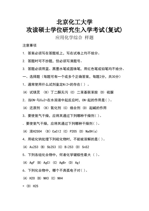
北京化工大学攻读硕士学位研究生入学考试(复试)应用化学综合样题注意事项1. 答案必须写在答题纸上,写在试卷上均不给分。
2. 答题时可不抄题,但必须写清题号。
3. 答题必须用蓝、黑墨水笔或圆珠笔,用红色笔或铅笔均不给分。
一、选择题(每题可有一个或多个正确答案,每题2分,共30分)1.通常使用什么试剂鉴定Ni2+的存在( ) 。
(A) 试镁灵(B)丁二酮无污 (C) 二苯基联苯胺 (D) 硫脲2.当CN-与Cu2+在水溶液中起反应时,CN-起的作用是( )。
(A) 还原剂(B)氧化剂 (C) 络合剂 (D) 起碱的作用3.要使氨气干燥,应将其通过下列哪种干燥剂( )。
.要使氨气干燥,应将其通过下列哪种干燥剂( )。
(A) 浓H2SO4 (B)CaCl2 (C) P2O5 (D) NaOH(s)4.用硫化钠处理下列硫化物时,不能被溶解的是( )。
(A) As2S3 (B) Sb2S3 (C) Bi2S3 (D) SnS25.下列各组化合物中,何者化学键极性最大 ( )。
(A) AgF (B) AgCl (C) AgBr (D) AgI6.下列化合物中,哪个不具孤电子对( )。
(A) H2O (B) NH3 (C) NH4+ (D) H2S7.下面一些宏观过程可看作可逆过程的有( )。
(A) 摩擦生热(B)0 oC 时冰熔化成水 (C) 电流通过金属发热 (D) 火柴燃烧8.把固体NaAc 加到HAc 稀溶液中,则pH 将( )。
(A)增高(B)不受影响 (C)下降 (D) 先下降后增高9. 反应:产物为物质B,若提高温度对产品产率有利,这表明活化能()。
(A) E1>E2, E1>E3 (B) E2>E1, E2>E3 (C) E1<E2, E1<E3 (D)E3>E1,E3>E210. 对于两组分系统能平衡共存的最多相数为()。
(A) 1 (B) 2 (C) 3 (D) 411. 设i 为理想混合气体中的一个组分,下面正确的是()(A) pi/p=Vi/V=ni/n (B) piV=pVi=niRT (C) piVi =niRT (D) 都正确12. 某液体混合物由状态A 变化到状态B,经历两条不同的途径,其热、功、内能变化、焓变化分别为Q1、W1、DU1、DH1 和Q2、W2、DU2、DH2,则()。
多势垒结构共振透射系数的计算

多势垒结构共振透射系数的计算骆敏;杨双波【摘要】The resonant transmission coefficient of multi-barrier structure is presented based on an exact solution of the Schrodinger equation by using the transfer matrix approach under the case of the incident electron energy being greater than, equal to, and less than the barrier height; furthermore, we have also studied the relationship between the resonant transmission coefficient,and the effective mass, the barrier width, and the number of barriers.%使用转移矩阵方法精确求解了一维定态薛定谔方程,求出了在多势垒结构中电子能量大于、等于、小于势垒高度情况下的共振透射系数的表达式,并进一步研究了多势垒结构的共振透射系数与有效质量和势垒宽度及势垒个数之间的关系.【期刊名称】《南京师大学报(自然科学版)》【年(卷),期】2012(035)002【总页数】6页(P50-55)【关键词】转移矩阵;共振透射系数;多势垒结构【作者】骆敏;杨双波【作者单位】南京师范大学物理科学与技术学院,江苏南京210046;南京师范大学物理科学与技术学院,江苏南京210046【正文语种】中文【中图分类】O413.1自从超晶格的概念[1]被提出来,同时由于分子束外延(MBE),金属氧化物沉积(MOCVD)[2]等制备超晶格技术的不断完善,超晶格被越来越多地研究[3-7].超晶格是一种由两种材料交替生长而成具有周期性的半导体结构,窄带隙的材料构成势阱,宽带隙的材料构成势垒[8].本文通过多势垒结构计算了透射系数及其与多势垒结构各参数之间的关系.1 模型与理论本文采用的多势垒结构如图1所示,其中,N为势垒的个数,v0为势垒高度,势垒和势阱中电子的有效质量分别为和,势垒和势阱宽度分别为a,b.在势垒和势阱区中直接求解一维薛定谔方程:图1 一维多势垒结构Fig.1 One dimensionalmulti-barrier structureN→为势垒的个数现我们假定具有一定能量的粒子由多势垒结构的最左边(x<0)向右方入射,则在1区有入射波和反射波,在2N+1区中由于没有由右向左运动的粒子,因此只有透射波(A2N+1≠0),没有向左传播的波(B2N+1=0),根据透射系数的定义[10]可得:2 计算结果和分析(1)有效质量的影响由图2知:随着有效质量的增大,产生共振透射的共振能量向低能量方向移动,各共振能量之间的间距随着有效质量的增大而减小,且势阱中的有效质量对共振能量的影响起主要作用.(2)势垒宽度的影响由图3知:随着势垒宽度的增大,逐渐形成微带、微带的宽度衰减、微带之间的间距逐渐增大,微带逐渐转变为一个透射峰.同时当势垒宽度增大到某一个值后,低能量位置的透射系数随势垒宽度的增大逐渐减小、共振透射峰消失,在低能量位置不再发生共振透射,高能量位置的微带变化比低能量位置的微带变化慢.(3)势垒个数的影响由图4知:随着势垒个数的增加,共振能量间距减小逐渐形成准连续微带,微带的宽度和微带之间的间距基本上不随势垒个数的变化而变化.对于N=5势垒结构来说,含有4个势阱,在低能量的位置出现4个峰,表明由于4个势阱之间的相互作用使最低能量态分裂成量子化能级.同理对于N=j势垒结构来说,含有(j-1)个势阱,在低能量位置会出现(j-1)个峰.图2 五势垒结构的透射系数与能量的关系图.有效质量为参数,势垒宽度(a=2 nm),势阱宽度(b=5nm),势垒高度(v0=0.5 eV)保持不变Fig.2 Transm ission coefficient as a function of incident electron energy for a five-barrier structure.The effectivem ass as aparameter.The barrier width (a=2 nm),thewellwidth (b=5nm),and the barrier height(v0=0.5 eV)remain unchanged3 结语利用一维薛定谔方程和转移矩阵推导了多势垒结构的透射系数的一般表达式,采用GaAs/Ga1-x Al x As的参数,计算了无偏压情况下5个、10个、15个、20个势垒结构的透射系数,并分析了势垒结构参数与共振能量之间的关系.计算结果表明:(a)发生共振透射的能量随有效质量和的增加逐渐向低能方向移动,且对共振能量的影响比对其影响大.(b)当势阱宽度一定时,势垒宽度是影响准连续微带的宽度和微带之间间距的主要因素,随着垒宽增大,微带宽度衰减,微带逐渐转变为一个透射峰,微带之间的间距增大.(c)势垒个数(N)与形成共振峰的个数(N-1)有直接关系,随着势垒个数的增加,共振能量间距减小逐渐形成准连续微带,微带的宽度和微带之间的间距基本上不随势垒个数的变化而变化.这些结果有利于我们对共振透射物理现象的理解及对实验和器件研究具有一定的参考和指导作用.图3 十五势垒结构的透射系数与能量的关系图.势垒宽度为参数,有效质量=0.108 5m0,w=0.067m0),势阱宽度(b=5nm),势垒高度(v0=0.5 eV)保持不变Fig.3 Transm ission coefficient as a function of incident electron energy for a fifteen-barrier structure.The barrier width as a param eter.The effectivemass =0.108 5m0,=0.067m0),the wellwid th (b=5nm),the barrier height(v0=0.5 eV)remain unchanged图4 多势垒结构透射系数与能量的关系图.势垒个数为参数,有效质量(=0.108 5m0,=0.067m0),势垒宽度(a=2 nm),势阱宽度(b=5nm),势垒高度(v0=0.5 eV)保持不变Fig.4 Transm ission coefficient as a function of incident electron energy for amulti-barrier structure.The number of barriers as a parameter,the effectivemass =0.108 5m0,0.067m0),the barrier width (a=2 nm),thewellwidth (b=5nm),the barrier height(v0=0.5 eV)remain unchanged[参考文献][1] Esaki L,Tsu R.Superlattice and negative differential conductivity in semiconductors[J].IBM JRes Develop,1970,14(1),61-65.[2]黄和鸾.半导体超晶格——材料与应用[M].沈阳:辽宁大学出版社,1992. [3] Tsu R,Esaki L.Tunneling in a finite superlattice[J].Appl Phys Lett,1973,22(11):562-564.[4] Chang L L,Esaki L,Tsu R.Resonant tunneling in semiconductor double barriers[J].Appl Phys Lett,1974,24(12):593-595.[5] Kelly M J.Tunnelling in quantum-well structures[J].Electronics Letters,1984,20(19):771-772.[6] VasellM O,Lee J,Lockwood H F.Multibarrier tunneling in Ga1-x Al x As/GaAs heterostructures[J].JAppl Phys,1983,54(9):5 206-5 213. [7] Rauch C,Strasser G,Unterrainer K,et al.Transition between coherent and incoherent electron transport in GaAs/GaAlAs superlattices [J].Phys Rev Lett,1998,81(16):3 495-3 498.[8]夏建白,朱邦芬.半导体超晶格物理[M].上海:上海科学技术出版社,1995. [9] Bastard G.Superlattice band structure in the envelope-function approximation[J].Phys Rev B,1981,24(10):5 693-5 697.[10]周世勋.量子力学教程[M].北京:高等教育出版社,2006.。
微扰理论及其应用
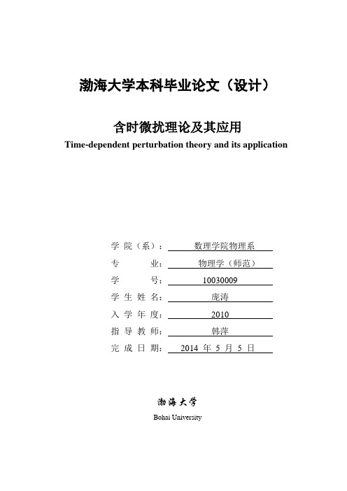
渤海大学本科毕业论文(设计)含时微扰理论及其应用Time-dependent perturbation theory and its application学院(系):数理学院物理系专业:物理学(师范)学号:10030009学生姓名:庞涛入学年度:2010指导教师:韩萍完成日期:2014 年5 月5 日渤海大学Bohai University摘要在量子力学中,精确求解薛定谔方程是很困难的,一般只能求近似解,应用微扰理论可以求得近似解。
学好微扰理论在以后的学习中具有很大帮助。
微扰理论分为两类,不含时微扰理论和含时微扰理论。
在量子力学中,含时微扰理论研究的是一个量子系统的含时微扰所产生的效应.该理论是由英国物理学家狄拉克首先提出和发展建立起来的。
应用含时微扰理论可以近似的计算出有微扰时的波函数,从而计算无微扰体系在微扰作用下由一个量子态跃迁到另一个量子态的跃迁概率。
含时微扰包括常微扰和周期微扰,在这两种微扰作用下,得到的结果是不同的,我们分析计算了在常微扰和周期微扰两种微扰作用下的跃迁概率,得到了一些结论。
在常微扰作用下时,我们得到了一个重要公式,该公式被称为费米黄金定则。
常微扰是只在一段时间内起作用,时间足够长的话,则跃迁概率与时间无关;而通过计算无微扰体系在周期微扰作用下的跃迁概率,得出的结论是周时,期微扰的频率只有在一定范围内,才会发生跃迁。
只有当外界微扰含有频率mk才会出现明显跃迁。
此外,我们还讨论了光的发射和吸收,给出了偶极跃迁的选择定则。
最后对激光的产生和激光的应用进行了介绍。
关键词:选择定则;含时微扰;跃迁概率;黄金规则Time-dependent perturbation theory and its applicationAbstractIn quantum mechanics, the exact solution of Schrodinger equation is very difficult, generally only approximate solutions, using the perturbation theory can be obtained the approximate solution. To learn a great help to the perturbation theory of learning in the future. Perturbation theory is divided into two categories, not the time-dependent perturbation theory and time-dependent perturbation theory.In quantum mechanics, the time-dependent theory of perturbation is the effect of a quantum system with time-dependent perturbation generated. This theory was first proposed and developed by the British physicist Dirac. Calculated using time-dependent perturbation theory can be approximated by a wave function perturbation, thus calculated without perturbation system under the perturbation induced by a quantum state transition to the transition probability of another quantum state. The time-dependent perturbation included regular perturbation and periodic perturbation, in which two kinds of perturbations, the result is different, analysis of transition probability in constant perturbation and periodic perturbation two perturbation effect was obtained by us, some conclusions were obtained. In the constant under perturbations, we obtain a formula, the formula is called the Fermi golden rule. The perturbation is often work only in a period of time, time is long enough, the transition probability is independent of time; and through the calculation of transition probability without perturbation system in the period under perturbations, it was concluded that the periodic perturbation frequency only in a certain range, the transition will occur. Only when the external perturbation with frequency, will appear obvious transition. In addition, we also discuss the emission and absorption of light, gives the dipole transition selection rule. Application of laser and laser produced finally is introduced in this paper.Key Words:Selection rule;time-dependent perturbation;transition probability;The golden rule目录摘要 (I)Abstract (II)引言 (1)1 含时微扰理论的概述 (2)1.1 含时微扰理论下的薛定谔方程 (2)1.2 跃迁概率 (3)2 常微扰和周期微扰 (5)2.1 跃迁概率和费米黄金定则 (5)2.2 周期微扰 (7)3 含时微扰理论的应用 (10)3.1 光的发射和吸收 (10)3.1.1 爱因斯坦的发射和吸收系数 (10)3.1.2 用微扰理论计算发射和吸收系数 (11)3.2 选择定则 (14)3.3 典例分析 (16)4 激光简介 (18)4.1 激光的产生 (18)4.2 激光的应用 (19)结论 (21)参考文献 (22)引言在量子力学中,对于具体物理问题的薛定谔方程,可以准确求解的问题是很少的,一般只能求近似解。
On the asymptotic expansion of the solutions of the separated nonlinear Schroedinger equati
a r X i v :n l i n /0012025v 3 [n l i n .S I ] 10 M a y 2001On the Asymptotic Expansion of the Solutions of the Separated Nonlinear Schr¨o dinger EquationA.A.Kapaev,St Petersburg Department of Steklov Mathematical Institute,Fontanka 27,St Petersburg 191011,Russia,V.E.Korepin,C.N.Yang Institute for Theoretical Physics,State University of New York at Stony Brook,Stony Brook,NY 11794-3840,USAAbstractNonlinear Schr¨o dinger equation with the Schwarzian initial data is important in nonlinear optics,Bose condensation and in the theory of strongly correlated electrons.The asymptotic solutions in the region x/t =O (1),t →∞,can be represented as a double series in t −1and ln t .Our current purpose is the description of the asymptotics of the coefficients of the series.MSC 35A20,35C20,35G20Keywords:integrable PDE,long time asymptotics,asymptotic expansion1IntroductionA coupled nonlinear dispersive partial differential equation in (1+1)dimension for the functions g +and g −,−i∂t g +=12∂2x g −+4g 2−g +,(1)called the separated Nonlinear Schr¨o dinger equation (sNLS),contains the con-ventional NLS equation in both the focusing and defocusing forms as g +=¯g −or g +=−¯g −,respectively.For certain physical applications,e.g.in nonlin-ear optics,Bose condensation,theory of strongly correlated electrons,see [1]–[9],the detailed information on the long time asymptotics of solutions with initial conditions rapidly decaying as x →±∞is quite useful for qualitative explanation of the experimental phenomena.Our interest to the long time asymptotics for the sNLS equation is inspired by its application to the Hubbard model for one-dimensional gas of strongly correlated electrons.The model explains a remarkable effect of charge and spin separation,discovered experimentally by C.Kim,Z.-X.M.Shen,N.Motoyama,H.Eisaki,hida,T.Tohyama and S.Maekawa [19].Theoretical justification1of the charge and spin separation include the study of temperature dependent correlation functions in the Hubbard model.In the papers[1]–[3],it was proven that time and temperature dependent correlations in Hubbard model can be described by the sNLS equation(1).For the systems completely integrable in the sense of the Lax representa-tion[10,11],the necessary asymptotic information can be extracted from the Riemann-Hilbert problem analysis[12].Often,the fact of integrability implies the existence of a long time expansion of the generic solution in a formal series, the successive terms of which satisfy some recurrence relation,and the leading order coefficients can be expressed in terms of the spectral data for the associ-ated linear system.For equation(1),the Lax pair was discovered in[13],while the formulation of the Riemann-Hilbert problem can be found in[8].As t→∞for x/t bounded,system(1)admits the formal solution given byg+=e i x22+iν)ln4t u0+∞ n=12n k=0(ln4t)k2t −(1t nv nk ,(2)where the quantitiesν,u0,v0,u nk and v nk are some functions ofλ0=−x/2t.For the NLS equation(g+=±¯g−),the asymptotic expansion was suggested by M.Ablowitz and H.Segur[6].For the defocusing NLS(g+=−¯g−),the existence of the asymptotic series(2)is proven by P.Deift and X.Zhou[9] using the Riemann-Hilbert problem analysis,and there is no principal obstacle to extend their approach for the case of the separated NLS equation.Thus we refer to(2)as the Ablowitz-Segur-Deift-Zhou expansion.Expressions for the leading coefficients for the asymptotic expansion of the conventional NLS equation in terms of the spectral data were found by S.Manakov,V.Zakharov, H.Segur and M.Ablowitz,see[14]–[16].The general sNLS case was studied by A.Its,A.Izergin,V.Korepin and G.Varzugin[17],who have expressed the leading order coefficients u0,v0andν=−u0v0in(2)in terms of the spectral data.The generic solution of the focusing NLS equation contains solitons and radiation.The interaction of the single soliton with the radiation was described by Segur[18].It can be shown that,for the generic Schwarzian initial data and generic bounded ratio x/t,|c−xthese coefficients as well as for u n,2n−1,v n,2n−1,wefind simple exact formulaeu n,2n=u0i n(ν′)2n8n n!,(3)and(20)below.We describe coefficients at other powers of ln t using the gener-ating functions which can be reduced to a system of polynomials satisfying the recursion relations,see(24),(23).As a by-product,we modify the Ablowitz-Segur-Deift-Zhou expansion(2),g+=exp i x22+iν)ln4t+i(ν′)2ln24t2] k=0(ln4t)k2t −(18t∞n=02n−[n+1t n˜v n,k.(4)2Recurrence relations and generating functions Substituting(2)into(1),and equating coefficients of t−1,wefindν=−u0v0.(5) In the order t−n,n≥2,equating coefficients of ln j4t,0≤j≤2n,we obtain the recursion−i(j+1)u n,j+1+inu n,j=νu n,j−iν′′8u n−1,j−2−−iν′8u′′n−1,j+nl,k,m=0l+k+m=nα=0, (2)β=0, (2)γ=0, (2)α+β+γ=ju l,αu k,βv m,γ,(6) i(j+1)v n,j+1−inv n,j=νv n,j+iν′′8v n−1,j−2++iν′8v′′n−1,j+nl,k,m=0l+k+m=nα=0, (2)β=0, (2)γ=0, (2)α+β+γ=ju l,αv k,βv m,γ,(7)where the prime means differentiation with respect toλ0=−x/(2t).Master generating functions F(z,ζ),G(z,ζ)for the coefficients u n,k,v n,k are defined by the formal seriesF(z,ζ)= n,k u n,k z nζk,G(z,ζ)= n,k v n,k z nζk,(8)3where the coefficients u n,k,v n,k vanish for n<0,k<0and k>2n.It is straightforward to check that the master generating functions satisfy the nonstationary separated Nonlinear Schr¨o dinger equation in(1+2)dimensions,−iFζ+izF z= ν−iν′′8zζ2 F−iν′8zF′′+F2G,iGζ−izG z= ν+iν′′8zζ2 G+iν′8zG′′+F G2.(9) We also consider the sectional generating functions f j(z),g j(z),j≥0,f j(z)=∞n=0u n,2n−j z n,g j(z)=∞n=0v n,2n−j z n.(10)Note,f j(z)≡g j(z)≡0for j<0because u n,k=v n,k=0for k>2n.The master generating functions F,G and the sectional generating functions f j,g j are related by the equationsF(zζ−2,ζ)=∞j=0ζ−j f j(z),G(zζ−2,ζ)=∞j=0ζ−j g j(z).(11)Using(11)in(9)and equating coefficients ofζ−j,we obtain the differential system for the sectional generating functions f j(z),g j(z),−2iz∂z f j−1+i(j−1)f j−1+iz∂z f j==νf j−z iν′′8f j−ziν′8f′′j−2+jk,l,m=0k+l+m=jf k f lg m,2iz∂z g j−1−i(j−1)g j−1−iz∂z g j=(12)=νg j+z iν′′8g j+ziν′8g′′j−2+jk,l,m=0k+l+m=jf kg l g m.Thus,the generating functions f0(z),g0(z)for u n,2n,v n,2n solve the systemiz∂z f0=νf0−z (ν′)28g0+f0g20.(13)The system implies that the product f0(z)g0(z)≡const.Since f0(0)=u0and g0(0)=v0,we obtain the identityf0g0(z)=−ν.(14) Using(14)in(13),we easilyfindf0(z)=u0e i(ν′)28n n!z n,4g0(z)=v0e−i(ν′)28n n!z n,(15)which yield the explicit expressions(3)for the coefficients u n,2n,v n,2n.Generating functions f1(z),g1(z)for u n,2n−1,v n,2n−1,satisfy the differential system−2iz∂z f0+iz∂z f1=νf1−z iν′′8f1−ziν′8g0−z(ν′)24g′0+f1g20+2f0g0g1.(16)We will show that the differential system(16)for f1(z)and g1(z)is solvable in terms of elementary functions.First,let us introduce the auxiliary functionsp1(z)=f1(z)g0(z).These functions satisfy the non-homogeneous system of linear ODEs∂z p1=iν4−ν′′4f′0z(p1+q1)−i(ν′)28−ν′g0,(17)so that∂z(q1+p1)=−(ν2)′′8z,p1(z)= −iνν′′8−ν′u′032z2,g1(z)=q1(z)g0(z),g0(z)=v0e−i(ν′)24−ν′′4v0 z+i(ν′)2ν′′4−ν′′4u0 ,v1,1=v0 iνν′′8−ν′v′0u n,2n −1=−2u 0i n −1(ν′)2(n −1)n −1ν′′u 0,n ≥2,v n,2n −1=−2v 0(−i )n −1(ν′)2(n −1)n −1ν′′v 0,n ≥2.Generating functions f j (z ),g j (z )for u n,2n −j ,v n,2n −j ,j ≥2,satisfy the differential system (12).Similarly to the case j =1above,let us introduce the auxiliary functions p j and q j ,p j =f jg 0.(21)In the terms of these functions,the system (12)reads,∂z p j =iνz(p j +q j )+b j ,(22)wherea j =2∂z p j −1+i (ν′)28−j −14(p j −1f 0)′8f 0+iν4−ν′′zq j −1−−ν′g 0+i(q j −2g 0)′′zj −1 k,l,m =0k +l +m =jp k q l q m .(23)With the initial condition p j (0)=q j (0)=0,the system is easily integrated and uniquely determines the functions p j (z ),q j (z ),p j (z )= z 0a j (ζ)dζ+iνzdζζζdξ(a j (ξ)+b j (ξ)).(24)These equations with expressions (23)together establish the recursion relationfor the functions p j (z ),q j (z ).In terms of p j (z )and q j (z ),expansion (2)readsg +=ei x22+iν)ln 4t +i(ν′)2ln 24tt2t−(18tv 0∞ j =0q j ln 24tln j 4t.(25)6Let a j (z )and b j (z )be polynomials of degree M with the zero z =0of multiplicity m ,a j (z )=M k =ma jk z k,b j (z )=Mk =mb jk z k .Then the functions p j (z )and q j (z )(24)arepolynomials of degree M +1witha zero at z =0of multiplicity m +1,p j (z )=M +1k =m +11k(a j,k −1+b j,k −1)z k ,q j (z )=M +1k =m +11k(a j,k −1+b j,k −1) z k.(26)On the other hand,a j (z )and b j (z )are described in (23)as the actions of the differential operators applied to the functions p j ′,q j ′with j ′<j .Because p 0(z )=q 0(z )≡1and p 1(z ),q 1(z )are polynomials of the second degree and a single zero at z =0,cf.(19),it easy to check that a 2(z )and b 2(z )are non-homogeneous polynomials of the third degree such thata 2,3=−(ν′)4(ν′′)2210(2+iν),(27)a 2,0=−iνν′′8−ν′u ′08u 0,b 2,0=iνν′′8−ν′v ′08v 0.Thus p 2(z )and q 2(z )are polynomials of the fourth degree with a single zero at z =0.Some of their coefficients arep 2,4=q 2,4=−(ν′)4(ν′′)24−(1+2iν)ν′′8u 0−ν(u ′0)24−(1−2iν)ν′′8v 0−ν(v ′0)22.Proof .The assertion holds true for j =0,1,2.Let it be correct for ∀j <j ′.Then a j ′(z )and b j ′(z )are defined as the sum of polynomials.The maximal de-grees of such polynomials are deg (p j ′−1f 0)′/f 0 =2j ′−1,deg (q j ′−1g 0)′/g 0 =72j′−1,anddeg 1z j′−1 α,β,γ=0α+β+γ=j′pαqβqγ =2j′−1. Thus deg a j′(z)=deg b j′(z)≤2j′−1,and deg p j′(z)=deg q j′(z)≤2j′.Multiplicity of the zero at z=0of a j′(z)and b j′(z)is no less than the min-imal multiplicity of the summed polynomials in(23),but the minor coefficients of the polynomials2∂z p j′−1and−(j−1)p j′−1/z,as well as of2∂z q j′−1and −(j−1)q j′−1/z may cancel each other.Let j′=2k be even.Thenm j′=min m j′−1;m j′−2+1;minα,β,γ=0,...,j′−1α+β+γ=j′mα+mβ+mγ =j′2 . Let j′=2k−1be odd.Then2m j′−1−(j′−1)=0,andm j′=min m j′−1+1;m j′−2+1;minα,β,γ=0,...,j′−1α+β+γ=j′mα+mβ+mγ =j′+12]p j,k z k,q j(z)=2jk=[j+12]z nn−[j+18k k!,g j(z)=v0∞n=[j+12]k=max{0;n−2j}q j,n−k(−i)k(ν′)2k2]k=max{0;n−2j}p j,n−ki k(ν′)2k2]k=max{0;n−2j}q j,n−k(−i)k(ν′)2kIn particular,the leading asymptotic term of these coefficients as n→∞and j fixed is given byu n,2n−j=u0p j,2j i n−2j(ν′)2(n−2j)n) ,v n,2n−j=v0q j,2j (−i)n−2j(ν′)2(n−2j)n) .(32)Thus we have reduced the problem of the evaluation of the asymptotics of the coefficients u n,2n−j v n,2n−j for large n to the computation of the leading coefficients of the polynomials p j(z),q j(z).In fact,using(24)or(26)and(23), it can be shown that the coefficients p j,2j,q j,2j satisfy the recurrence relationsp j,2j=−i (ν′)2ν′′2jj−1k,l,m=0k+l+m=jp k,2k p l,2l q m,2m++ν(ν′)2ν′′4j2j−1k,l,m=0k+l+m=jp k,2k(p l,2l−q l,2l)q m,2m,q j,2j=i (ν′)2ν′′2jj−1k,l,m=0k+l+m=jp k,2k q l,2l q m,2m−(33)−ν(ν′)2ν′′4j2j−1k,l,m=0k+l+m=jp k,2k(p l,2l−q l,2l)q m,2m.Similarly,the coefficients u n,0,v n,0for the non-logarithmic terms appears from(31)for j=2n,and are given simply byu n,0=u0p2n,n,v n,0=v0q2n,n.(34) Thus the problem of evaluation of the asymptotics of the coefficients u n,0,v n,0 for n large is equivalent to computation of the asymptotics of the minor coeffi-cients in the polynomials p j(z),q j(z).However,the last problem does not allow a straightforward solution because,according to(8),the sectional generating functions for the coefficients u n,0,v n,0are given byF(z,0)=∞n=0u n,0z n,G(z,0)=∞n=0v n,0z n,and solve the separated Nonlinear Schr¨o dinger equation−iFζ+izF z=νF+18zG′′+F G2.(35)93DiscussionOur consideration based on the use of generating functions of different types reveals the asymptotic behavior of the coefficients u n,2n−j,v n,2n−j as n→∞and jfixed for the long time asymptotic expansion(2)of the generic solution of the sNLS equation(1).The leading order dependence of these coefficients on n is described by the ratio a n2+d).The investigation of theRiemann-Hilbert problem for the sNLS equation yielding this estimate will be published elsewhere.Acknowledgments.We are grateful to the support of NSF Grant PHY-9988566.We also express our gratitude to P.Deift,A.Its and X.Zhou for discussions.A.K.was partially supported by the Russian Foundation for Basic Research under grant99-01-00687.He is also grateful to the staffof C.N.Yang Institute for Theoretical Physics of the State University of New York at Stony Brook for hospitality during his visit when this work was done. References[1]F.G¨o hmann,V.E.Korepin,Phys.Lett.A260(1999)516.[2]F.G¨o hmann,A.R.Its,V.E.Korepin,Phys.Lett.A249(1998)117.[3]F.G¨o hmann,A.G.Izergin,V.E.Korepin,A.G.Pronko,Int.J.Modern Phys.B12no.23(1998)2409.[4]V.E.Zakharov,S.V.Manakov,S.P.Novikov,L.P.Pitaevskiy,Soli-ton theory.Inverse scattering transform method,Moscow,Nauka,1980.[5]F.Calogero,A.Degasperis,Spectral transforms and solitons:toolsto solve and investigate nonlinear evolution equations,Amsterdam-New York-Oxford,1980.[6]M.J.Ablowitz,H.Segur,Solitons and the inverse scattering trans-form,SIAM,Philadelphia,1981.10[7]R.K.Dodd,J.C.Eilbeck,J.D.Gibbon,H.C.Morris,Solitons andnonlinear wave equations,Academic Press,London-Orlando-San Diego-New York-Toronto-Montreal-Sydney-Tokyo,1982.[8]L.D.Faddeev,L.A.Takhtajan,Hamiltonian Approach to the Soli-ton Theory,Nauka,Moscow,1986.[9]P.Deift,X.Zhou,Comm.Math.Phys.165(1995)175.[10]C.S.Gardner,J.M.Greene,M.D.Kruskal,R.M.Miura,Phys.Rev.Lett.19(1967)1095.[11]x,Comm.Pure Appl.Math.21(1968)467.[12]V.E.Zakharov,A.B.Shabat,Funkts.Analiz Prilozh.13(1979)13.[13]V.E.Zakharov,A.B.Shabat,JETP61(1971)118.[14]S.V.Manakov,JETP65(1973)505.[15]V.E.Zakharov,S.V.Manakov,JETP71(1973)203.[16]H.Segur,M.J.Ablowitz,J.Math.Phys.17(1976)710.[17]A.R.Its,A.G.Izergin,V.E.Korepin,G.G.Varzugin,Physica D54(1992)351.[18]H.Segur,J.Math.Phys.17(1976)714.[19]C.Kim,Z.-X.M.Shen,N.Motoyama,H.Eisaki,hida,T.To-hyama and S.Maekawa Phys Rev Lett.82(1999)802[20]A.R.Its,SR Izvestiya26(1986)497.11。
氦原子基态的Schrodinger方程的严格解

氦原子基态的Schrodinger 方程的严格解物理0701班徐振桓摘要 本文利用了超球坐标的方法求解了氦原子基态的Schrodinger 方程的严格解,得出了氦原子的基态能量和波函数。
关键词 超球坐标 氢原子基态 Schrodinger 方程严格求解三体或三体以上体系的Schrodinger 方程是量子理论工作者非常感兴趣的重要 课题。
原因在于,可得到体系的真实波函数,进而可研究电子相关等许多物理和化学问题。
自从量子力学建立,人们就期待着这一问题的解决,直到将超球坐标用来描写多粒子 Schrodinger 方程,多体问题才变得可能解决。
在这条道路上,前人已做了许多努力,但仍存在一些问题。
本文给出一个新的方法来严格求解氦原子的基态能量和波函数。
这一方法也可用于氦原 子激发态和其它原子能态的计算,原则上可用之求解任意多体问题。
本文计算证明了 Schro dinger 方程可以描写三粒子体系,可作为严格求解多体 Schrodinger 方程的一个范例。
对氦原子,原子单位下的非相对论Schrodinger 方程为:2123123111(,,)(,,),2ji j ii i jiij z z r r r E r r r m r ψψ=<⎧⎫⎪⎪-∇+=⎨⎬⎪⎪⎩⎭∑∑(1) 其中i m 为i 粒子的质量,i z 为 i 粒子荷电数 (电子为一1,核为2)。
本文采取 smith 的坐标 取法:先引人三个Euler 角 (α,β,γ) 以描写此原子在空定坐标中的取向,然后在三粒 子所张的平面上用,1r ,2r 分别为电子1,2距核的距离)和两个角度θ和ϕ 描写电子与核的相对位置。
这些量与直角坐标的关系为:i x = R cos θcos 12(ϕ+i β),0≤θ≤4π,i y = R sin θsin12(ϕ+i β),0≤ϕ≤2π, i=1,2, (2)这里 132πβ=,232πβ=-。
引人这三个坐标的主要优点在于Euler 角可以直接引出总角动量 ,而不需再对角动量进行标准化耦合。
- 1、下载文档前请自行甄别文档内容的完整性,平台不提供额外的编辑、内容补充、找答案等附加服务。
- 2、"仅部分预览"的文档,不可在线预览部分如存在完整性等问题,可反馈申请退款(可完整预览的文档不适用该条件!)。
- 3、如文档侵犯您的权益,请联系客服反馈,我们会尽快为您处理(人工客服工作时间:9:00-18:30)。
(8)
m′ m
2
Therefore, the energy eigenvalues and corresponding wave functions for the potential V (y ) as En and φn (y ) become ˜n = En E and 1 φ n (y ) m(x) (10)
(2)
+ (f ′ ) V (f (x))
1 d2 f ′′ m′ − − − 2 dx2 m 2f ′
2
1 m′′ d m′ − ′ + (α − 1) dx 2 m m
2
m′ − m
f ′′ f′ (3)
ψ (x) = (f ′ )2 E ψ (x), 2
where the prime denotes differentiation with respect to x. On the other hand the one dimensional Schr¨ odinger equation with position dependent mass can be written as − 1 dψ (x) 1 d ˜ (x)ψ (x) = Eψ ˜ (x), +V 2 dx M (x) dx (4)
Exact solution of Schr¨ odinger equation for modified Kratzer’s molecular potential with the position-dependent mass
arXiv:0712.0268v1 [quant-ph] 3 Dec 2007
.
(9)
ψn (x) =
(11)
3
Applications
We solve Schr¨ odinger equation exactly for two potentials the rotationally corrected Morse potential[30] and the modified Kratzer molecular potential[31]. We consider three kinds of the position dependent mass distributions. Two of them are used before[19], and the third one is the exponentially decreasing mass distribution with a free parameter q.
Ramazan Sever 1, Cevdet Tezcan
1
2
Middle East Technical University,Department of Physics, 06531 Ankara, Turkey
2 Faculty
of Engineering, Ba¸ skent University, Ba˜ glıca Campus, Ankara, Turkey
Comparing Eqs. (3) and (5), we get the following identities f ′′ m′ m′ − = 2f ′ m 2m and
′′ ′2 ′ ˜ (x) − E ˜ = f [V (f (x)) − E ] − 1 m − m V m 2m m m
(6)
1
1
Introduction
Solutions of Schr¨ odinger equation for a given potential with any angular momentum have much attention in chemical physics systems. Energy eigenvalues and the corresponding eigenfunctions provide a complete information about the diatomic molecules. Morse and Kratzer potentials [1,2] are one of the well-known diatomic potentials. The method used in the Schr¨ odinger equation for vibration-rotation states are mostly based on the wave function expansion and exact solution for a single state with some restrictions on the coupling constants [3-7]. On the other hand solutions of the position-dependent effective-mass Schr¨ odinger equation are very interesting chemical potential problem. They have also found important applications in the fields of material science and condensed matter physics such as semiconductors[8], quantum well and quantum dots[9], 3 H , clusters[10], quantum liquids[11], graded alloys and semiconductor heterostructures]12,13]. Recently, number of exact solutions on these topics increased[14-31]. Various methods are used in the calculations. The point canonical transformations (PCT) is one of these methods providing exact solutions of energy eigenvalues and corresponding eigenfunctions [24-27]. It is also used for solving the Schr¨ odinger equation with position-dependent effective mass for some potentials [8-13]. In the present work, we solve two different potentials with the three mass distributions. The point canonical transformation is taken in the more general form introducing a free parameter. This general form of the transformation will provide us a set of solutions for different values of free parameter. In this work, the exact solution of Schr¨ odinger equation is obtained or the modified Kratzer type of molecular potential [31] and the corrected Morse potential [32]. The contents of the paper is as follows. In section 2, we present briefly the solution of the Schr¨ odinger by using point canonical transformation. In section 3, we introduce some applications for the specific mass distributions. Results are discussed in section 4.
3
3.1
Modified Kratzer Potential
2
y − ye , (12) y where De is the dissociation energy and ye is the equilibrium internuclear separation. Energy spectrum and the wave functions are V (r ) = De h ¯ 4µDe ye 2µ h ¯2
f ′′ f′
(7)
From Eq. (6), one gets f ′ = m1/2 Substituting f ′ into Eq. (7), the new potential can be obtained as
′′ ˜ (x) = V (f (x)) − 1 m − 7 V 8m m 4
February 2, 2008
Abstract Exact solutions of Schr¨ odinger equation are obtained for the modified Kratzer and the corrected Morse potentials with the position-dependent effective mass. The bound state energy eigenvalues and the corresponding eigenfunctions are calculated for any angular momentum for target potentials. Various forms of point canonical transformations are applied. PACS numbers: 03.65.-w; 03.65.Ge; 12.39.Fd Keywords: Morse potential, Kratzer potential, Position-dependent mass, Point canonical transformation, Effective mass Schr¨ odinger equation.