Lec9--hypothesis testing

合集下载

氯化血红素模拟酶催化柱后衍生高效液相色谱荧光检测法测定染发剂中的过氧化氢

广东化工2019年第3期·178 · 第46卷总第389期氯化血红素模拟酶催化-柱后衍生-高效液相色谱-荧光检测法测定染发剂中的过氧化氢李锦花1，李赛花2，马明1，陈丹超1，许海峰3，郭蓓霖3，吴坚3，陈威威3 (1．宁波检验检疫科学技术研究院，浙江宁波315012；2．宁波诺丁汉大学，浙江宁波315100；3．宁波中盛产品检测有限公司，浙江宁波315100)Determination of Hydrogen Peroxide in Hair Dye by Post-column Derivatization-High Performance Chromatography with Fluorescence Detection Li Jinhua1，Li Saihua2, Ma Ming1, Chen Danchao1, Xu Haifeng3, Guo Peilin3, Chen Weiwei3, Wu Jian3(1. Ningbo Academy of Inspection and Quarantine Science and Technology, Ningbo 315012；2. University of Nottingham Ningbo China, Ningbo315100；3. Ningbo Joysun Product Testing Co., Ltd., Ningbo 315100, China)Abstract: The method for determination of hydrogen peroxide in hair dye by post-column derivatization-high performance chromatography with fluorescence detection was developed based on the reaction which the p-hydroxyphenylacetic acid can be oxidized to the fluorescent dimer by hydrogen peroxide with hemin as catalyzer. The most derivatization efficiency was obtained with the hemin and p-hydroxyphenylacetic acid concentration at 8 μmol·L-1and 80 μmol·L-1, respectively, with the derivatization reagent pH at 10.5 and the derivatization temperature at 35℃. The linear ranger between 0.005 μmol/l~50 μmol/l was observed for the established method. The sample detection limit was 0.3 mg·kg-1and standard spike recoveries was 98.2~98.6 % under the optimized conditions. The obvious advantages of excellent anti-jamming capability and high-sensitivity were observed comparing with other methods for determination of benzoyl peroxide.Keywords: Post-column Derivatization；High Performance Chromatography；Fluorescence Detection；Hair Dye；Hydrogen Peroxide1 引言过氧化氢(HPO, hydrogen peroxide)是一种最重要的过氧化物之一，也是最简单的过氧化物，与水、甲醇和乙醇等溶剂互溶。

注射用水系统验证方案

上海****药业有限公司二〇一八年二月验证方案的起草、审核和批准目录1概述 (7)1.1设备概述 (7)1.2设备主要技术参数： (7)2水系统工艺流程 (7)2.1注射用水系统工艺流程说明 (7)2.2注射用水系统工艺流程图....................................................................................................... ..8 2.3 注射用水系统五车间各取样点示意图.. (9)2.4 注射用水系统六车间各取样点示意图 (10)2.5 注射用水系统七车间各取样点示意图 (11)3验证的目的和适用范围 (12)3.1验证目的 (12)3.2适用范围 (12)3.3验证内容 (12)3.4验证时间 (12)4职责 (12)4.1验证小组职责 (12)4.2验证领导小组职责 (12)5验证的管理 (13)5.1偏差及变更 (13)5.2参考文献 (13)5.3人员 (13)6验证准备工作 (14)6.1设备的风险分析 (14)6.2改造方案的确认 (14)6.3仪器、仪表的确认 (15)6.4设备文件确认 (15)6.5改造安装确认 (15)6.6注射用水系统技术参数的确认 (16)6.7预处理系统的确认 (16)6.8双级反渗透的确认 (16)6.9注射用水储罐的确认 (17)6.10注射用水循环泵的确认 (17)6.11水的流速 (18)6.12换热器的确认 (18)6.13紫外灯的确认 (18)6.14设备材质及阀门的确认 (19)6.15环路系统 (19)6.16自动控制系统 (20)6.17注射用水输送管路的确认 (20)6.18系统现场条件的确认 (21)6.19公用系统连接的确认 (21)6.20设备备品、备件的确认 (21)6.21改造安装确认报告 (22)7运行确认 (22)7.1安装确认完成确认 (22)7.2操作规程确认 (22)7.3水泵的确认 (23)7.4电气控制系统及显示仪表的确认 (23)7.5系统及循环管路泄漏的确认 (24)7.6原水、注射用水的水温自动控制系统确认 (24)7.7系统性能运行测试 (24)7.8断电恢复测试 (25)7.9注射用水管路流速确认 (26)7.10反渗透机组高压泵低压、高压保护的确认 (26)7.11系统储罐液位自动控制的确认 (27)7.12注射用水产水自动控制的确认 (27)7.13开关、按钮的确认 (28)7.14运行确认报告 (28)8 性能确认 (28)8.1性能确认前准备 (28)8.2取样计划 (29)8.3注射用水质量确认 (30)9.4清洗消毒效果 (31)8.5注射用水系统性能确认报告 (31)9再验证周期 (31)10验证最终审核批准 (31)11设备验证系统文件管理 (31)11.1文件归档： (31)11.2文件使用： (31)11.3文件保存期限： (31)附件1 (33)设备风险分析 (33)附件 2 (35)改造方案确认 (35)附件3 (37)人员列表 (37)附件4 (38)仪器仪表的确认 (38)附件5 (39)设备文件确认 (39)附件6 (40)注射用水技术参数确认 (40)附件7 (41)预处理系统的确认 (41)附件8 (42)注射用水储罐的确认 (43)附件10 (44)注射用水循环泵的确认 (44)附件11 (45)水的流速 (45)附件12 (46)换热器的确认 (46)附件13 (47)紫外灯的确认 (47)附件14 (48)设备材质及阀门的确认 (48)附件15 (49)环路系统 (49)附件16 (50)自动控制系统 (50)附件17 (51)注射用水输送管路的确认 (51)附件18 (52)系统现场条件的确认 (52)附件19 (53)公用系统的确认 (53)附件20 (54)设备备品、备件的确认 (54)附件21 (55)改造安装确认报告 (55)附件22 (56)运行前准备 (56)附件23 (57)操作规程的确认 (57)附件24 (58)水泵的确认 (58)附件25 (59)电气控制系统及显示仪表的确认 (59)附件26 (60)系统及循环管路泄漏的确认 (60)附件27 (61)原水、注射用水水温自动控制确认 (61)附件28 (62)系统性能运行测试 (62)附件29 (63)断电恢复测试 (63)附件30 (64)反渗透机组高压泵低压、高压保护的确认 (65)附件32 (66)系统储罐液位自动控制的确认 (66)附件33 (67)注射用水产水的自动控制确认 (67)附件34 (68)开关、按钮的确认 (68)附件35 (69)运行确认报告 (69)附件36 (70)确认前准备 (70)附件37 (72)注射用水系统运行关键参数统计........................................................ (72)附件38 (81)性能确认报告 (81)附件39 (82)偏差列表 (82)附件40 (83)变更列表 (83)附件41 (84)再验证周期 (84)附件42 (85)验证合格批准书 (86)1 概述1.1 设备概述该注射用水制备系统安装在大容量注射剂十六车间注射用水制备间，采用纯化水制备系统生产的纯化水为源水，用工业蒸汽作为热源，经LD6000/6A型多效蒸馏水机蒸馏的方法获得，质量符合《中国药典》2010版二部标准，存储于20吨注射用水储罐，并经两路循环系统输送至各使用点，分别为大容量注射剂六车间注射用水循环系统、大容量注射剂五车间注射用水循环系统。

五氯苯酚检测标准技术分析与展望

检测认证五氯苯酚检测标准技术分析与展望■ 宋玉峰（山东省产品质量检验研究院）摘要：五氯苯酚因其防霉杀菌作用广泛应用于多个领域，在保护消费品品质的同时存在潜在健康风险。

科学有效地检测识别这类物质是了解与防范其安全风险的基础。

本文梳理了国内外五氯苯酚痕量迁移物现行检测标准，概述并比较其迁移物提取的前处理实验流程和检测技术方法，通过前处理流程及检测技术的梳理解析，分析比较过程的复杂性和操控性、试剂的环保性，探讨实验技术的优化及改进。

本文以期为五氯苯酚检测过程中绿色环保的改进、提高检测过程的可操控性等提供参考。

关键词：五氯苯酚，有害物质迁移，前处理技术，健康风险DOI编码：10.3969/j.issn.1002-5944.2023.15.036Prospect and Technological Analysis of DetectionStandard for trace pentachlorophenol MigrationSONG Yu-feng（Shandong Institute for Product Quality Inspection）Abstract:Pentachlorophenol is extensively applied in many fields due to its anti-bacterial and anti-fungal effects, which facilitates the quality of products and has health risks. Effective identification of these substances is the basis of understanding and preventing safety risks. The paper sorts out current detection standards to trace phentachlorophenol migration at home and abroad. The paper presents and compares the pretreatment experimental processes and technological testing methods, analyzes the complexity, controllability, and environmental effects of reagents by sorting out pretreatment processes and testing methods, and discusses the improvement of experimental technologies. The paper provides reference for improving the greenness and controllability of pentachlorophenol detection process.Keywords: pentachlorophenol, migration of harmful substances, pretreatment technology, health risk0 引言五氯苯酚及其盐和酯类物质防霉杀菌效果好，价格优势明显，使用方便，作除草剂、防腐剂和防霉剂广泛用于多个领域。

ADDT包：加速破坏性坏化测试数据分析的标准方法说明书

Package‘ADDT’October12,2022Type PackageTitle Analysis of Accelerated Destructive Degradation Test DataVersion2.0Date2016-10-08Author Yili Hong,Yimeng Xie,Zhongnan Jin,and Caleb KingMaintainer Yili Hong<***************>Description Accelerated destructive degradation tests(ADDT)are often used to collect neces-sary data for assessing the long-term properties of polymeric materials.Based on the col-lected data,a thermal index(TI)is estimated.The TI can be useful for material rating and com-parison.This package implements the traditional method based on the least-squares method,the parametric method based on maximum likelihood estimation,and the semi-parametric method based on spline methods,and the corresponding methods for estimat-ing TI for polymeric materials.The traditional approach is a two-step approach that is cur-rently used in industrial standards,while the parametric method is widely used in the statisti-cal literature.The semiparametric method is newly developed.Both the parametric and semi-parametric approaches allow one to do statistical inference such as quantifying uncertain-ties in estimation,hypothesis testing,and predictions.Publicly available datasets are provided il-lustrations.More details can be found in Jin et al.(2017).License GPL-2Depends nlme,Matrix,coneprojRoxygenNote5.0.1.9000NeedsCompilation noRepository CRANDate/Publication2016-11-0320:12:52R topics documented:ADDT-package (2)addt.conﬁnt.ti.mle (3)addt.ﬁt (4)addt.mean.summary (6)addt.predint.ybar.mle (7)12ADDT-package AdhesiveBondB (8)AdhesiveFormulationK (9)plot.addt.ﬁt (9)PolymerY (10)SealStrength (10)summary.addt.ﬁt (11)Index13 ADDT-package Accelerated Destructive Degradation TestingDescriptionAccelerated destructive degradation tests(ADDT)are often used to collect necessary data for as-sessing the long-term properties of polymeric materials.Based on the collected data,a thermal index(TI)is estimated.The TI can be useful for material rating and comparisons.This package implements the traditional method based on the least-squares method,the parametric method based on maximum likelihood estimation,and the semiparametric method based on spline methods,and their corresponding methods for estimating TI for polymeric materials.The traditional approach is a two-step approach that is currently used in industrial standards,while the parametric method is widely used in the statistical literature.The semiparametric method is newly developed.The parametric and semiparametric approaches allow one to do statistical inference such as quantify-ing uncertainties in estimation,hypothesis testing,and predictions.Publicly available datasets are provided for illustrations.More details can be found in Jin et al.(2017).DetailsPackage:ADDTType:PackageVersion: 2.0Date:2016-10-08License:GPL-2Author(s)Yili Hong,Yimeng Xie,Zhongnan Jin,and Caleb KingMaintainer:Yili Hong<***************>ReferencesC.B.King,Y.Xie,Y.Hong,J.H.Van Mullekom,S.P.DeHart,and P.A.DeFeo,“A compari-son of traditional and maximum likelihood approaches to estimating thermal indices for polymeric materials,”Journal of Quality Technology,in press,2016.addt.conﬁnt.ti.mle3L.A.Escobar,W.Q.Meeker,D.L.Kugler,and L.L.Kramer,“Accelerated destructive degradation tests:Data,models,and analysis,”in Mathematical and Statistical Methods in Reliability,B.H.Lindqvist and K.A.Doksum,Eds.River Edge,NJ:World Scientiﬁc Publishing Company,2003, ch.21.M.Li and N.Doganaksoy,“Batch variability in accelerated-degradation testing,”Journal of Quality Technology,vol.46,pp.171-180,2014.Y.Xie,C.B.King,Y.Hong,and Q.Yang,“Semi-parametric models for accelerated destructive degradation test data analysis,”Preprint:arXiv:1512.03036,2015.Y.Xie,Z.Jin,Y.Hong,and J.H.Van Mullekom,“Statistical methods for thermal index estimation based on accelerated destructive degradation test data,”in Statistical Modeling for Degradation Data,D.G.Chen,Y.L.Lio,H.K.T.Ng,and T.R.Tsai,Eds.NY:New York:Springer,2017,ch.12.Z.Jin,Y.Xie,Y.Hong,and J.H.Van Mullekom,“ADDT:An R package for analysis of accelerated destructive degradation test data,”in Statistical Modeling for Degradation Data,D.G.Chen,Y.L.Lio,H.K.T.Ng,and T.R.Tsai,Eds.NY:New York:Springer,2017,ch.14.addt.confint.ti.mle Conﬁdence Interval for Thermal Index(TI).DescriptionComputes a conﬁdence interval for the TI.Usageaddt.confint.ti.mle(obj,conflevel)Argumentsobj An addt.fit object.conflevel Conﬁdence level in decimal form(i.e.,95%is0.95)ValueReturns a vector containing the estimated TI,standard error,and lower and upper conﬁdence limits.NoteThis currently only implements the CI procedure for ML approach.See Alsoaddt.fitaddt.fit ADDT Model FittingDescriptionFits degradation data using the least-squares,maximum likelihood,and semiparametric methodsand estimates the thermal indices(TI).Usageaddt.fit(formula,data,initial.val=100,proc="All",failure.threshold,time.rti=1e+05,method="Nelder-Mead",subset,na.action,starts=NULL,fail.thres.vec=c(70,80),semi.control=list(cor=F,...),...)Argumentsformula A formula of type Response~Time+Temperature.The order of Time and Tem-perature cannot be changed.data A data frame contains the ADDT data to be analyzed.initial.val We need response measurements at time point0to compute the initial degrada-tion level in the model.If the data does not contain that information,user mustsupply the initial.value.Otherwise,the function will give an error message.proc The type of analysis to be performed which can be"LS"(least squares),"ML"(maximum likelihood),"SemiPara"(semiparametric),or"All"(the least-squares,maximum likelihood and semiparametric methods).failure.thresholdThe value below which a soft failure occurs.Must be in the form of a percent ofthe initial value.time.rti The time associated with the thermal index(TI)or relative thermal index(RTI).Typically100,000hours.method An argument passed to optim specifying the optimization procedure.Default isNelder-Mead.subset An optional statement that allows the use of only part of the dataset.na.action Indicates the action required when data contain missing values.starts A vector of starting values for the maximum likelihood procedure.See fail.thres.vec for alternative.fail.thres.vec If the user does not specify“starts”argument,the user may specify a vectorof two different failure.thresholds.The least-squares procedure is then used forthe two different failure.thresholds to produce starting values for the maximumlikelihood procedure.semi.control list=(cor=F,...),control parameters related to the semiparametric method.If notspeciﬁed,default is no correlation.When cor=T in the list is speciﬁed,modelassumes a correlation term....Optional arguments.DetailsA thermal index(TI)or relative thermal index(RTI)is often used to evaluate long-term perfor-mance of polymeric materials.Accelerated destructive degradation testing(ADDT)is widely used to calculate the TI of certain polymeric materials.The dataset considered in addt.ﬁt function contain repeated measurements of a response,say tensile strength,at some combinations of time and temperature.The least squares procedure aggregates data into the average of measurements at each combination of time and temperature.Then,polynominal regression is used to interpolate the failure time for each combination.A least squares line isﬁtted to the failure time data and the TI is then obtained byT I=beta1log10(time.rti)−beta0−273.16.It is important to note that observations are required after failure in order for this procedure to be successful.The maximum likelihood procedure assumes a degradation path dependent on time and temperature.An example of a parametric form for this path can be found in Vaca-Trigo and Meeker(2009)and is the form currently used here.The error term is assumed to follow a multivariate normal distribution.A TI can be directly estimated from the parameter estimates for the degradation path.The addt.fitfunction will be generalized to allow other parametric forms of the mean function,and/or other non-Guassian distribution in later versions.The semiparametric model assembles both parametric model like Arrhenius model for degradation variable extrapolation as well as non-parametric model in order to be more compatible for various materials.ValueAn object of class"addt.ﬁt",which is a list containing:LS.obj If least-squares approach is used,a LS.obj will returned.It contains estimates of coefﬁcients in the TI formula,estimated TI,a matrix contains the failure timeby polynomial interpolation.ML.obj A ML.obj object is returned if maximum likelihood approach is speciﬁed.SemiPara.obj A SemiPara.obj is returned if SemiPara approach is speciﬁed.dat The data set used in least square/maximum likelihood approaches.time.rti An argument stored to be used for functions related to"addt.ﬁt"object.initial.val An argument stored to be used for functions related to"addt.ﬁt"object.failure.thresholdAn argument stored to be used for functions related to"addt.ﬁt"object. ReferencesY.Hong,C.B.King,Y.Xie,J.H.Van Mullekom,S.P.Dehart,and P.A.DeFeo(2014).“A Comparison of Least Squares and Maximum Likelihood Approaches to Estimating Thermal Indices for Polymeric Materials,”Journal of Quality Technology,in press,2016.6addt.mean.summaryI.Vaca-Trigoand,W.Q.Meeker,“A statistical model for linkingﬁeld and laboratory exposureresults for a model coating,”in Service Life Prediction of Polymeric Materials,J.Martin,R.A.Ryntz,J.Chin,and R.A.Dickie,Eds.NY:New York:Springer,2009,ch.2.Y.Xie,C.B.King,Y.Hong,and Q.Yang,“Semi-parametric models for accelerated destructive degradation test data analysis,”Preprint:arXiv:1512.03036,2015.See Alsoplot.addt.ﬁt,summary.addt.ﬁtExamplesdata(AdhesiveBondB)##Least Squaresaddt.fit.lsa<-addt.fit(Response~TimeH+TempC,data=AdhesiveBondB,proc="LS",failure.threshold=70)##Maximum Likelihoodaddt.fit.mla<-addt.fit(Response~TimeH+TempC,data=AdhesiveBondB,proc="ML",failure.threshold=70)##Semiparametric##Not run:addt.fit.semi<-addt.fit(Response~TimeH+TempC,data=AdhesiveBondB,proc="SemiPara", failure.threshold=70)##End(Not run)##All LS,ML and Semi-Parametric procedures##Not run:addt.fit.all<-addt.fit(Response~TimeH+TempC,data=AdhesiveBondB,proc="All", failure.threshold=70)##End(Not run)summary(addt.fit.lsa)summary(addt.fit.mla)##Not run:summary(addt.fit.semi)##Not run:summary(addt.fit.all)##Not run:plot(addt.fit.all,type="data")##Not run:plot(addt.fit.all,type="LS")##Not run:plot(addt.fit.all,type="ML")##Not run:plot(addt.fit.semi,type="SEMI")##Not run:addt.confint.ti.mle(addt.fit.mla,conflevel=0.95)addt.mean.summary ADDT Batch Means SummaryDescriptionFunction that returns the averaged responses for each time-temperature batch.addt.predint.ybar.mle7Usageaddt.mean.summary(dat)Argumentsdat A dataframe contains the measurements from the ADDT.The dataframe con-tains temperature,time,and response from left to right.ValueReturns a dataframe giving the mean response for each time-temperature batch.ReferencesY.Hong,C.B.King,Y.Xie,J.H.Van Mullekom,S.P.Dehart,and P.A.DeFeo(2014).“A Comparison of Least Squares and Maximum Likelihood Approaches to Estimating Thermal Indices for Polymeric Materials,”Journal of Quality Technology,in press,2016.Examplesdata(AdhesiveBondB)addt.mean.summary(AdhesiveBondB)addt.predint.ybar.mle Prediction of the mean of future observationsDescriptionGiven observations for one temperature level up to some time point,computes a prediction interval for the mean degradation level at some future time point.Usageaddt.predint.ybar.mle(obj,conflevel,num.fut.obs=5,temp,tt)Argumentsobj An addt.fit object.conflevel The conﬁdence level of the prediction interval.This argument is in decimal form(i.e.,95%is0.95).num.fut.obs The number of future observations within a batch at the future time point.temp The temperature level at which predictions are to be made.tt The future time point where prediction is desired.ValueReturns a vector containing the lower and upper bounds of the prediction interval.8AdhesiveBondB NoteThis function only works with an object resulted from ML approach.ReferencesY.Hong,C.B.King,Y.Xie,J.H.Van Mullekom,S.P.Dehart,and P.A.DeFeo(2014).“A Comparison of Least Squares and Maximum Likelihood Approaches to Estimating Thermal Indices for Polymeric Materials,”Journal of Quality Technology,in press,2016.See Alsoaddt.fitAdhesiveBondB Adhesive Bond B datasetDescriptionA dataset from Escobar et al.(2003)containing the results of an accelerated destructive degradationtesting on the strength of an adhesive bond.Usagedata(AdhesiveBondB)FormatA data frame with82observations on the following3variables.TempC Temperature.TimeH Time in hours.Response Strength(Newtons).SourceL.A.Escobar,W.Q.Meeker,D.L.Kugler,and L.L.Kramer,“Accelerated destructive degradation tests:Data,models,and analysis,”in Mathematical and Statistical Methods in Reliability,B.H.Lindqvist and K.A.Doksum,Eds.River Edge,NJ:World Scientiﬁc Publishing Company,2003, ch.21.AdhesiveFormulationK9 AdhesiveFormulationK Adhesive Formulation K DataDescriptionA dataset from Xie al.(2015)Strength was tested at40,50,and60degree C.Usagedata(AdhesiveFormulationK)FormatA data frame with101observations on the following3variables.TempC Temperature.TimeH Time in hours.Response Strength(Newtons).SourceY.Xie,C.B.King,Y.Hong,and Q.Yang(2015).Semiparametric Models for Accelerated Destruc-tive Degradation Test Data Analysis.Preprint:arXiv:1512.03036.plot.addt.fit ADDT PlottingDescriptionProvides graphical tools for ADDT analysis.Usage##S3method for class addt.fitplot(x,type,...)Argumentsx An addt.ﬁt object.type Type of plot("data","ML","LS","SEMI")to be generated.If type="data",a scatter plot of the dataset in addt.ﬁt object is generated.If type="ML",a plotof data along with the results of ML approach is produced.If type="LS",thepolynominalﬁt to the data is plotted.If type="SEMI",the semi-parametricﬁt tothe data is plotted....Optional arguments.10SealStrengthSee Alsoaddt.fitPolymerY Polymeric MaterialDescriptionA dataset from Tsai et al.(2013)conducting a study on the tensile strength of a new type of polymermaterial.Usagedata(PolymerY)FormatA data frame with76observations on the following3variables.TempC Temperature.TimeH Time in hours.Response Strength(Newtons).SourceTsai,C.-C.,S.-T.Tseng,N.Balakrishnan,and C.-T.Lin(2013).Optimal design for accelerated destructive degradation tests.Quality Technology and Quantitative Management10,263-276. SealStrength Data for Seal StrengthDescriptionSeal Strength dataset presented in Li and Doganaksoy(2014).In the R package ADDT,Seal Strength dataset has minor modiﬁcations where the temperature at time point0is changed to200degree where in the original dataset,it is100degree.This is a computing trick that will not affect the model results.Usagedata(SealStrength)FormatA data frame with210observations on the following3variables.TempC Temperature.TimeH Time in hours.Response Strength(Newtons)DetailsSeal strength dataset is collected under an experiment of testing the strength of a new seal. SourceM.Li,and N.Doganaksoy(2014).Batch variability in accelerated-degradation testing.Journal of Quality Technology46,171-180.summary.addt.fit Summary of an"addt.ﬁt"object.DescriptionProvides a brief summary of an addt.ﬁt object.Usage##S3method for class addt.fitsummary(object,...)Argumentsobject An addt.fit object....Optional arguments.ValueReturns a list whose items vary depending on which procedure was used in addt.ﬁt.If proc="ML", then the output has the following items:coef.mle.mat A matrix giving the estimated coefﬁcients,their standard errors,and the lower and upper bounds of a95%conﬁdence interval.ti.CI The estimated thermal index of the material,its standard error,and95%conﬁ-dence interval.logLik The maximum log-likelihood value achieved.If proc="LS",the output has the following items:coefs A vector giving the estimated coefﬁcients for the time-temperature line.TI The estimated thermal index of the material.interp.time A matrix contains the interpolated time at the failure.threshold speciﬁed for each temperature level.If proc="SemiPara",the output has the following items:betahat An estimate of our model coefﬁcient under the users chosen setups.knots Knots used in the B-spline,these are the optimal knots if best.knots=TRUE.Loglik The maximum log-likelihood value achieved.aic aic value for theﬁnal model.aicc aicc value for theﬁnal model.If proc="All",the output will give the preceeding values for all the LS.obj,ML.obj and Semi-Para.obj.See Alsoaddt.fitIndex∗packageADDT-package,2ADDT(ADDT-package),2ADDT-package,2addt.confint.ti.mle,3addt.fit,3,4,5,8,10–12addt.mean.summary,6addt.predint.ybar.mle,7 AdhesiveBondB,8 AdhesiveFormulationK,9optim,4plot.addt.fit,6,9PolymerY,10SealStrength,10summary.addt.fit,6,1113。

中和抗体检测应用于新型冠状病毒mRNA_疫苗效力分析

国家药监局重点实验室专栏[重点实验室简介]国家药品监督管理局生物制品质量研究与评价重点实验室是国家药监局２０１９年首批认定的重点实验室ꎬ依托单位为中国食品药品检定研究院生物制品检定所ꎮ生物制品检定所主要开展应用基础研究ꎬ方向包括:治疗类生物技术产品㊁预防类菌苗/疫苗及其创新性产品和一些重要的体内外诊断试剂(血液筛查)的质量控制和质量评价研究ꎻ建立符合国际规范的质量检定用标准物质㊁生产与检定用菌种库和细胞库等ꎮ通过提供疫苗及生物技术产品等国家标准物质㊁建立标准的检验技术㊁研究与制定完善的药品质量标准ꎬ生物制品检定所在我国药品质量控制㊁创新性药品研究与产业化发展中起到不可或缺的技术支撑作用ꎮ生物制品质量研究与评价重点实验室具备完善的生物制品检验检测体系ꎬ检测技术范围与检测能力在国内相同领域是唯一的也是最全面的ꎬ共获得的ＣＮＡＳ实验室资质认定的项目２２２项ꎮ２０１３年生物制品检定所被评估认定成为ＷＨＯ生物制品标准化和评价合作中心ꎬ２０１７年通过ＷＨＯ生物制品标准化和评价合作中心再认定ꎮ通过广泛的国际药交流(ＷＨＯ㊁英国ＮＩＢＳＣ㊁美国药学会㊁美国ＦＤＡ和人用药物注册技术要求国际协调会议ＩＣＨ等)ꎬ重点实验室不仅引进国外先进的药品质量监管理念和技术ꎬ还将我国的一些优势技术运用于国际标准品和国际药品质量标准的建立中ꎬ在相关领域的国际标准制定中发挥重要作用ꎮ实验室主任:徐苗ꎬ女ꎬ医学博士ꎬ研究员ꎬ博士生导师ꎬ中国食品药品检定研究院生物制品检定所所长ꎮ主要从事疫苗等生物制品质量控制与评价的研究和管理工作ꎮ先后主持国家级课题４项ꎬ参与省部级以上课题６项ꎬ以第一或通信作者在«Ｎａｔｕｒａｌｐｒｏｔｏｃｏｌｓ»«ＥｍｅｒｇｉｎｇＭｉｃｒｏｂｅｓ＆Ｉｎｆｅｃｔｉｏｎｓ»等杂志上发表论文８０余篇ꎬ编写专著５部ꎬ获授权专利６项ꎬ其中３项已经完成转化ꎬ先后获得中华预防医学会科学技术一等奖㊁中国防痨协会科学技术奖一等奖㊁中国药学会科学技术奖二等奖㊁北京市科学技术二等奖等多个奖项ꎮ获国家市场监管总局抗击新冠疫情先进个人㊁中国药学会以岭生物青年生物奖等ꎮ㊀基金项目:国家重点研发计划(Ｎｏ.２０２１ＹＦＣ２３０２４０４)作者简介:吴小红ꎬ女ꎬ硕士ꎬ副研究员ꎬ研究方向:新型冠状病毒ｍＲＮＡ疫苗及狂犬病疫苗质量控制ꎬＥ－ｍａｉｌ:ｗｕｘｉａｏｈｏｎｇ＠ｎｉｆｄｃ.ｏｒｇ.ｃｎ通信作者:刘欣玉ꎬ男ꎬ博士ꎬ研究员ꎬ研究方向:疫苗质量控制ꎬＴｅｌ:０１０－５３８５１７８０ꎬＥ－ｍａｉｌ:ｌｉｕｘｉｎｙｕ＠ｎｉｆｄｃ.ｏｒｇ.ｃｎ中和抗体检测应用于新型冠状病毒ｍＲＮＡ疫苗效力分析吴小红ꎬ赵丹华ꎬ所玥ꎬ彭沁华ꎬ王红玉ꎬ刘欣玉ꎬ李玉华(中国食品药品检定研究院虫媒病毒疫苗室ꎬ国家药品监督管理局生物制品质量研究与评价重点实验室ꎬ北京１０２６２９)摘要:目的㊀通过对新型冠状病毒(２０１９ｎｏｖｅｌｃｏｒｏｎａｖｉｒｕｓꎬ２０１９－ｎＣｏＶ)ｍＲＮＡ疫苗(新冠ｍＲＮＡ疫苗)免疫小鼠后产生的中和抗体进行检测ꎬ探索中和抗体检测法应用于ｍＲＮＡ疫苗体内效力评价的可行性ꎮ方法㊀采用６~８周ＢＡＬＢ/ｃ小鼠进行后肢肌肉免疫ꎬ检测不同免疫剂量和不同免疫程序的中和抗体滴度ꎮ并对８家企业生产的新冠ｍＲＮＡ疫苗免疫的小鼠血清进行中和抗体和ＩｇＧ抗体检测ꎮ结果㊀２㊁５㊁１０μｇ不同剂量ｍＲＮＡ疫苗按照不同免疫程序免疫小鼠后中和抗体检测结果显示ꎬ抗体阳转率均为１００％ꎬ中和抗体反应有明显的剂量－效应关系ꎮ２针间隔１４ｄ加强免疫组抗体滴度显著高于间隔７ｄ加强免疫组及１针组(Ｆ＝５７.１３ꎬＰ<０.００１)ꎮ２μｇ剂量间隔７ｄ加强免疫和间隔１４ｄ加强免疫产生的中和抗体几何平均滴度(ｇｅｏｍｅｔｒｉｃｍｅａｎｔｉｔｅｒꎬＧＭＴ)分别为２１８和４６８ꎬ差异有统计学意义(ｔ＝３.４０ꎬＰ＝０.００３)ꎻ５μｇ剂量间隔７ｄ加强免疫和间隔１４ｄ加强免疫产生的中和抗体ＧＭＴ分别为４９９和１４３６ꎬ差异有统计学意义(ｔ＝３.６２ꎬＰ＝０.００２)ꎻ１０μｇ剂量间隔７ｄ加强免疫和间隔１４ｄ加强免疫产生的中和抗体ＧＭＴ分别为６０８和１９０９ꎬ差异有统计学意义(ｔ＝３.２３ꎬＰ＝０.００５)ꎮ国内８家企业生产的新冠ｍＲＮＡ疫苗免疫小鼠后均可产生高滴度的ＩｇＧ抗体(１０４.５~１０７.５)和中和抗体(１０２.６~１０４.８)ꎬ效力测定结果均符合企业质量标准ꎮ各企业生产的ｍＲＮＡ疫苗的中和抗体滴度结果差异有统计学意义(Ｆ＝７０.０３ꎬＰ<０.００１)ꎮ结论㊀小鼠免疫后中和抗体检测可用于ｍＲＮＡ疫苗的体内效力评价ꎮ关键词:新型冠状病毒ꎻｍＲＮＡ疫苗ꎻ中和抗体ꎻＩｇＧ抗体ꎻ效力中图分类号:Ｒ９１７㊀文献标志码:Ａ㊀文章编号:２０９５－５３７５(２０２３)１１－０８９６－００６ｄｏｉ:１０.１３５０６/ｊ.ｃｎｋｉ.ｊｐｒ.２０２３.１１.００９ＳｔｕｄｙｏｎｔｈｅｐｏｔｅｎｃｙｏｆｍＲＮＡＣＯＶＩＤ－１９ｖａｃｃｉｎｅｉｎｖｉｖｏｕｓｉｎｇｎｅｕｔｒａｌｉｚｉｎｇａｎｔｉｂｏｄｙａｓｓａｙＷＵＸｉａｏｈｏｎｇꎬＺＨＡＯＤａｎｈｕａꎬＳＵＯＹｕｅꎬＰＥＮＧＱｉｎｈｕａꎬＷＡＮＧＨｏｎｇｙｕꎬＬＩＵＸｉｎｙｕꎬＬＩＹｕｈｕａ(ＮＭＰＡＫｅｙＬａｂｏｒａｔｏｒｙｆｏｒＱｕａｌｉｔｙＣｏｎｔｒｏｌａｎｄＥｖａｌｕａｔｉｏｎｏｆＢｉｏｌｏｇｉｃａｌＰｒｏｄｕｃｔｓꎬＤｉｖｉｓｉｏｎｏｆＡｒｂｏｖｉｒｕｓＶａｃｃｉｎｅꎬＮａｔｉｏｎａｌＩｎｓｔｉｔｕｔｅｓｆｏｒＦｏｏｄａｎｄＤｒｕｇＣｏｎｔｒｏｌꎬＢｅｉｊｉｎｇ１０２６２９ꎬＣｈｉｎａ)Ａｂｓｔｒａｃｔ:Ｏｂｊｅｃｔｉｖｅ㊀ＴｏｅｖａｌｕａｔｅｔｈｅｐｏｔｅｎｃｙｏｆｍＲＮＡＣＯＶＩＤ－１９ｖａｃｃｉｎｅｉｎｖｉｖｏｂｙｎｅｕｔｒａｌｉｚｉｎｇａｎｔｉｂｏｄｙａｓｓａｙａｆ￣ｔｅｒｍｉｃｅｉｍｍｕｎｉｚａｔｉｏｎꎬａｎｄｅｓｔａｂｌｉｓｈａｍｅｔｈｏｄｆｏｒｅｖａｌｕａｔｉｎｇｔｈｅｅｆｆｉｃａｃｙｏｆｔｈｅｖａｃｃｉｎｅ.Ｍｅｔｈｏｄｓ㊀ＢＡＬＢ/ｃｍｉｃｅａｔ６~８ｗｅｅｋｓｗｅｒｅｉｍｍｕｎｉｚｅｄｗｉｔｈｍＲＮＡＣＯＶＩＤ－１９ｖａｃｃｉｎｅａｎｄｔｈｅｎｅｕｔｒａｌｉｚｉｎｇａｎｔｉｂｏｄｙｔｉｔｅｒｓｏｆｄｉｆｆｅｒｅｎｔｉｍｍｕｎｅｄｏｓａｇｅａｎｄｄｉｆｆｅｒｅｎｔｖａｃｃｉｎａｔｉｏｎｓｃｈｅｄｕｌｅｓｗｅｒｅｄｅｔｅｃｔｅｄ.Ｔｈｅｖａｒｉａｎｔｖａｃｃｉｎｅｓｐｒｏｄｕｃｅｄｂｙｄｉｆｆｅｒｅｎｔｍａｎｕｆａｃｔｕｒｅｓｗｅｒｅｉｍｍｕｎｉｚｅｄａｔｉｎｔｅｒｖａｌｓｏｆ７ｄｏｒ１４ｄꎬａｎｄｓｅｒｕｍｓａｍｐｌｅｓｗａｓｃｏｌｌｅｃｔｅｄａｔ７ｄａｆｔｅｒｔｈｅｓｅｃｏｎｄｄｏｓｅｏｆｉｍｍｕｎｉｚａｔｉｏｎ.２０１９ｎｏｖｅｌｃｏｒｏｎａｖｉｒ￣ｕｓ(２０１９－ｎＣｏＶ)ｎｅｕｔｒａｌｉｚｉｎｇａｎｔｉｂｏｄｙｔｉｔｅｒａｎｄＩｇＧａｎｔｉｂｏｄｙｔｉｔｅｒｗｅｒｅｄｅｔｅｃｔｅｄｂｙｐｓｅｕｄｏｖｉｒｕｓｎｅｕｔｒａｌｉｚａｔｉｏｎｔｅｓｔａｎｄｅｎ￣ｚｙｍｅｌｉｎｋｅｄｉｍｍｕｎｏｓｏｒｂｅｎｔａｓｓａｙｓｅｐａｒａｔｅｌｙ.Ｒｅｓｕｌｔｓ㊀Ｔｈｅｒｅｓｕｌｔｓｏｆｎｅｕｔｒａｌｉｚｉｎｇａｎｔｉｂｏｄｙａｔｄｉｆｆｅｒｅｎｔｉｍｍｕｎｅｄｏｓａｇｅｏｆ２ꎬ５ꎬ１０μｇｍＲＮＡｖａｃｃｉｎｅｓｈｏｗｅｄｔｈａｔｔｈｅｓｅｒｏｐｏｓｉｔｉｖｅｒａｔｅｏｆａｎｔｉｂｏｄｙｉｎｍｉｃｅｗａｓ１００％ａｎｄｔｈｅｎｅｕｔｒａｌｉｚｉｎｇａｎｔｉｂｏｄｙｒｅａｃ￣ｔｉｏｎｈａｄａｎｏｂｖｉｏｕｓｄｏｓｅ－ｅｆｆｅｃｔｃｏｒｒｅｌａｔｉｏｎ.Ｔｈｅｎｅｕｔｒａｌｉｚａｔｉｏｎａｎｔｉｂｏｄｙｔｉｔｅｒｏｆｔｈｅ１４－ｄａｙｉｎｔｅｒｖａｌｇｒｏｕｐｗａｓｓｉｇｎｉｆｉｃａｎｔｌｙｈｉｇｈｅｒｔｈａｎｔｈａｔｏｆｔｈｅ７－ｄａｙｉｎｔｅｒｖａｌｇｒｏｕｐａｎｄｏｎｅｄｏｓｅｇｒｏｕｐ(Ｆ＝５７.１３ꎬＰ<０.００１).Ｔｈｅｇｅｏｍｅｔｒｉｃｍｅａｎｔｉｔｅｒｓ(ＧＭＴ)ｏｆｎｅｕｔｒａｌｉｚｉｎｇａｎｔｉｂｏｄｙｉｎｄｕｃｅｄｂｙ２μｇｄｏｓａｇｅｉｎｔｅｒｖａｌｏｆ７－ｄａｙａｎｄ１４－ｄａｙｗｅｒｅ２１８ａｎｄ４６８ꎬｒｅｓｐｅｃｔｉｖｅｌｙꎬｗｉｔｈｓｉｇｎｉｆｉ￣ｃａｎｔｄｉｆｆｅｒｅｎｃｅ(ｔ＝３.４０ꎬＰ＝０.００３)ꎻＴｈｅＧＭＴｏｆｎｅｕｔｒａｌｉｚｉｎｇａｎｔｉｂｏｄｙｉｎｄｕｃｅｄｂｙ５μｇｄｏｓａｇｅｉｎｔｅｒｖａｌｏｆ７－ｄａｙａｎｄ１４－ｄａｙｗｅｒｅ４９９ａｎｄ１４３６ꎬｒｅｓｐｅｃｔｉｖｅｌｙꎬｗｉｔｈｓｉｇｎｉｆｉｃａｎｔｄｉｆｆｅｒｅｎｃｅ(ｔ＝３.６２ꎬＰ＝０.００２)ꎻＴｈｅＧＭＴｏｆｎｅｕｔｒａｌｉｚｉｎｇａｎｔｉｂｏｄｉｅｓｉｎｄｕｃｅｄｂｙ１０μｇｄｏｓａｇｅｉｎｔｅｒｖａｌｏｆ７－ｄａｙａｎｄ１４－ｄａｙｗｅｒｅ６０８ａｎｄ１９０９ｒｅｓｐｅｃｔｉｖｅｌｙꎬｗｉｔｈｓｉｇｎｉｆｉｃａｎｔｄｉｆｆｅｒｅｎｃｅ(ｔ＝３.２３ꎬＰ＝０.００５).ＨｉｇｈｌｅｖｅｌｓｏｆＩｇＧａｎｔｉｂｏｄｙ(１０４.５~１０７.５)ａｎｄｎｅｕｔｒａｌｉｚｉｎｇａｎｔｉｂｏｄｙ(１０２.６~１０４.８)ｃｏｕｌｄｂｅｄｅｔｅｃｔｅｄａｆｔｅｒｉｍｍｕｎｉｚｉｎｇｍｉｃｅｗｉｔｈｔｈｅＣＯＶＩＤ－１９ｍＲＮＡｖａｃｃｉｎｅꎬｐｏｔｅｎｃｙｏｆｔｈｅｖａｃｃｉｎｅｓｗｅｒｅａｌｌｍｅｔｗｉｔｈｔｈｅｒｅｑｕｉｒｅｍｅｎｔｓｗｉｔｈｇｏｏｄｌｏｔｃｏｎｓｉｓｔｅｎｃｅꎬｔｈｅｒｅｗｅｒｅｓｉｇｎｉｆｉｃａｎｔｄｉｆｆｅｒｅｎｃｅｉｎｔｈｅａｎｔｉｂｏｄｙｔｉｔｅｒｓａｍｏｎｇｔｈｅｖａｒｉｏｕｓｖａｃｃｉｎｅｐｒｏｄｕｃｅｄｂｙｄｉｆｆｅｒｅｎｔｍａｎ￣ｕｆａｃｔｕｒｅｒｓ(Ｆ＝７０.０３ꎬＰ<０.００１).Ｃｏｎｃｌｕｓｉｏｎ㊀ＴｈｅｎｅｕｔｒａｌｉｚｉｎｇａｎｔｉｂｏｄｙｔｅｓｔｏｆｔｈｅｍｉｃｅａｆｔｅｒｉｍｍｕｎｉｚａｔｉｏｎｃａｎｂｅｕｓｅｄｔｏｅｖａｌｕａｔｅｔｈｅｐｏｔｅｎｃｙｏｆＣＯＩＤ－１９ｍＲＮＡｖａｃｃｉｎｅｉｎｖｉｖｏ.Ｋｅｙｗｏｒｄｓ:２０１９ｎｏｖｅｌｃｏｒｏｎａｖｉｒｕｓꎻｍＲＮＡｖａｃｃｉｎｅꎻＮｅｕｔｒａｌｉｚｉｎｇａｎｔｉｂｏｄｙꎻＩｇＧａｎｔｉｂｏｄｙꎻＰｏｔｅｎｃｙ㊀㊀新型冠状病毒感染(ｃｏｒｏｎａｖｉｒｕｓｄｉｓｅａｓｅ２０１９ꎬＣＯＶＩＤ－１９)的流行对人类健康造成了严重影响ꎮ疫苗接种已被证实对严重疾病㊁降低住院率和死亡率非常有效[１－２]ꎮ其中ｍＲＮＡ疫苗由于具有能够同时诱导体液免疫和细胞免疫㊁研发和生产周期短㊁容易实现量产等优势ꎬ成为国际上主要采用的ＣＯＶＩＤ－１９疫苗研发技术ꎮ随着新型冠状病毒(２０１９－ｎＣｏＶ)变异株的不断出现ꎬ单价变异株疫苗及多价变异株疫苗可作为加强免疫以及异源序贯免疫来应对病毒变异造成的感染威胁[３]ꎮ新冠ｍＲＮＡ疫苗的效力评价目前尚无国际标准ꎬ欧洲及世界卫生组织(ＷＨＯ)专家多推荐体外活性研究作为该疫苗效力评价的主要方法[４－６]ꎮ鉴于ｍＲＮＡ疫苗为创新技术疫苗ꎬ缺乏系统的疫苗质量研究经验ꎬ我国现阶段采用体内和体外双效力指标进行评价[７]ꎬ体内效力的评价可利用动物免疫后检测中和抗体和/或总抗体的方法来进行[８]ꎮ本研究对新冠ｍＲＮＡ疫苗不同免疫剂量和不同免疫程序诱导的中和抗体反应进行初步研究ꎬ并对新冠变异株ｍＲＮＡ疫苗及二价ｍＲＮＡ疫苗免疫小鼠后的抗体阳性率和抗体水平进行体内效力分析ꎬ从而评价ｍＲＮＡ疫苗的质量ꎮ１㊀材料与方法１.１㊀实验动物㊀ＳＰＦ级ＢＡＬＢ/ｃ小鼠ꎬ６~８周龄ꎬ体重１８~２２ｇꎬ雌雄不限ꎬ由中国食品药品检定研究院动物所提供ꎬ实验动物生产许可证号:ＳＣＸＫ(京)２０２２－０００２ꎬ使用许可证号:ＳＹＸＫ(京)２０２２－００１４ꎬ动物实验伦理批准文号:中检动(福)第２０２２(Ｂ)００８号ꎮ１.２㊀主要试剂及仪器㊀１０ˑＰＢＳ㊁ＴＭＢ㊁终止液购自索莱宝公司ꎻＨＲＰ标记的羊抗小鼠ＩｇＧ购自美国Ｊａｃｋｓｏｎ公司ꎻＢＳＡ购自美国Ｓｉｇｍａ公司ꎻＤＭＥＭ㊁胎牛血清㊁胰酶㊁ＨＥＰＥＳ㊁双抗均购自美国Ｇｉｂｃｏ公司ꎻ荧光素酶检测试剂购自美国普洛麦格Ｐｒｏｍｅｇａ公司ꎻＰｒｏｍｅｇａＧｌｏＭａｘ９６微孔板化学发光检测仪(Ｇｌｏｍａｘｎａｖｉｇａｔｏｒ)购自美国普洛麦格Ｐｒｏｍｅｇａ公司ꎻ酶标仪(ＩｎｆｉｎｉｔｅＭ２００)购自美国蒂肯公司ꎮ１.３㊀实验用疫苗㊁细胞㊁不同型别假病毒㊀实验用疫苗为国内企业生产的ｍＲＮＡ疫苗ꎬ编号Ｖ１~Ｖ９ꎮ其中Ｖ１为原型株疫苗ꎬＶ２~Ｖ７为二价２０１９－ｎＣｏＶ变异株ｍＲＮＡ疫苗(ＯｍｉｃｒｏｎＢＡ.４/５株和Ｄｅｌｔａ株双价㊁ＯｍｉｃｒｏｎＢＡ.４/５株和Ｂｅｔａ株双价㊁ＯｍｉｃｒｏｎＢＡ.２株和原型株双价以及ＯｍｉｃｒｏｎＸＢＢ.１.５株和ＢＱ.１.７株双价)ꎬＶ８~Ｖ９是２０１９－ｎＣｏＶ变异株ｍＲＮＡ疫苗(ＯｍｉｃｒｏｎＢＡ.１)ꎻＶｅｒｏ细胞购自ＡＴＣＣꎬ本室传代保存ꎻ假病毒原型株㊁Ｄｅｌｔａ株㊁Ｂｅｔａ株㊁Ｏ￣ｍｉｃｒｏｎＢＡ.１㊁ＯｍｉｃｒｏｎＢＡ.２㊁ＯｍｉｃｒｏｎＢＡ.４/５㊁ＯｍｉｃｒｏｎＸＢＢ.１.５购自北京云菱生物技术公司ꎻ不同株２０１９－ｎＣｏＶＳ蛋白抗原分别购自北京义翘神州生物技术有限公司和北京百普赛斯公司ꎮ１.４㊀免疫剂量及免疫程序１.４.１㊀ｍＲＮＡ疫苗免疫剂量和免疫程序研究㊀将Ｖ１ｍＲＮＡ疫苗(原型株)配制成不同浓度后ꎬ按照不同的免疫程序分成Ａ㊁Ｂ㊁Ｃ３组:Ａ组程序为免疫１针ꎬ１４ｄ采血ꎻＢ组程序为间隔７ｄ加强免疫１针后７ｄ采血ꎻＣ组程序为间隔１４ｄ加强免疫１针后７ｄ采血ꎮ每种免疫程序按照不同的免疫剂量分成３个小组ꎬ分别是每只小鼠注射２㊁５和１０μｇꎬ共计９组ꎬ每组１０只小鼠ꎮ同时１０只小鼠注射生理盐水作为阴性对照组ꎮ每只小鼠后肢肌肉注射１００μＬ疫苗ꎬ眼球取血分离血清ꎬ－２０ħ保存备用ꎮ用假病毒中和试验法检测抗２０１９－ｎＣｏＶ中和抗体ꎮ１.４.２㊀实验疫苗免疫和检测㊀ｍＲＮＡ变异株疫苗及二价疫苗均按照企业的免疫剂量和免疫程序进行免疫和采血ꎬ分离血清后于－２０ħ保存ꎮ分别进行中和抗体和ＩｇＧ结合抗体的检测ꎮ１.５㊀假病毒中和试验(ＰＢＮＡ法)㊀按照操作规程进行[９－１０]ꎬ在９６孔板上３倍系列稀释的血清１００μＬꎬ分别加入各型假病毒[用ＤＭＥＭ培养基稀释至１.３ˑ１０４半数组织培养感染剂量(ＴＣＩＤ５０)/ｍＬ]ꎬ每孔加入５０μＬꎬ同时设立病毒对照和细胞对照ꎮ３７ħ５％ＣＯ２培养箱中和１ｈꎬ加入２ˑ１０５个/ｍＬ的Ｖｅｒｏ细胞悬液ꎬ每孔１００μＬꎬ３７ħ５％ＣＯ２培养箱培养２０~２８ｈ后ꎬ从细胞培养箱中取出９６孔板ꎬ用多道移液器从每个上样孔中吸弃１５０μＬ上清ꎬ然后加入１００μＬ荧光素酶检测试剂ꎬ室温避光反应２ｍｉｎꎮ反应结束后ꎬ用多道移液器将反应孔中的液体反复吹吸６~８次ꎬ使细胞充分裂解ꎬ从每孔中吸出１００μＬ液体ꎬ加于对应９６孔化学发光检测板中ꎬ置于化学发光检测仪中读取发光值ꎮ计算抑制率＝{１－[样品组的发光强度均值－空白对照ＣＣ(ＣｅｌｌＣｏｎｔｒｏｌꎬＣＣ)均值]/[阴性组的发光强度ＶＣ(ＶｉｒｕｓＣｏｎｔｒｏｌꎬＶＣ)均值－空白对照值ＣＣ均值]}ˑ１００％ꎮ根据中和抑制率结果ꎬ按照ＲｅｅｄＭｕｅｎｃｈ法计算中和抗体滴度半数效应剂量(５０％ｍａｘｉｍａｌｅｆｆｅｃｔｉｖｅｃｏｎｃｅｎｔｒａｔｉｏｎꎬＥＣ５０)ꎬＥＣ５０>３０为抗体阳性ꎮ１.６㊀特异性抗２０１９－ｎＣｏＶＳｐｉｋｅ蛋白ＩｇＧ抗体检测㊀将２０１９－ｎＣｏＶ各株抗原分别用１ˑＰＢＳ稀释至２μｇｍＬ－１ꎬ取９６孔板每孔加１００μＬꎬ(５ʃ３)ħ条件下包被过夜１６ｈꎬＰＢＳＴ洗板３次ꎬ拍干后加入封闭液(２％ＢＳＡ溶液)ꎬ１００μＬ/孔ꎬ３７ħ孵箱里封闭２ｈꎬ加入系列稀释后的待检测血清样本ꎬ３７ħ孵箱里孵育后１ｈꎬＰＢＳＴ洗板３次ꎬ加入辣根过氧化物酶(ＨＲＰ)标记的羊抗小鼠ＩｇＧ抗体ꎬ每孔１００μＬꎬ３７ħ孵育后１ｈꎬＰＢＳＴ洗板３次ꎬ加入底物ＴＭＢ５０μＬꎬ室温避光显色３~５ｍｉｎꎬ加入１ｍｏｌＬ－１硫酸溶液终止液终止ꎬ１５０μＬ/孔ꎬ在酶标仪上检测波长４５０ｎｍ/６３０ｎｍ的ＯＤ值ꎬ以阴性小鼠吸光度均值的２.１倍为ｃｕｔｏｆｆ值ꎮ血清Ａ值大于ｃｕｔｏｆｆ值为抗体阳性ꎬ取阳性Ａ值最大的血清稀释度为血清的ＩｇＧ抗体滴度ꎮ１.７㊀统计学方法㊀使用ＧｒａｐｈＰａｄＰｒｉｓｍ８.０进行数据分析ꎬ相同免疫剂量不同免疫程序以及相同免疫程序不同免疫剂量间中和抗体滴度以及不同企业ｍＲＮＡ疫苗免疫后中和抗体之间比较采用单因素方差分析评估组间差异ꎬ中和抗体和ＩｇＧ抗体之间差异采用ｔ检验分析ꎬＰ<０.０５表示差异有统计学意义ꎮ２㊀结果２.１㊀不同免疫剂量和不同免疫程序的抗体反应㊀针对原型株ｍＲＮＡ疫苗不同免疫剂量和免疫程序的中和抗体检测结果显示ꎬ２㊁５㊁１０μｇｍＲＮＡ疫苗免疫小鼠后ꎬ１针免疫组和２针免疫组抗体阳性率均为１００％ꎮ２㊁５㊁１０μｇ首针免疫后１４ｄ或２１ｄ中和抗体反应具有明显的剂量－效应关系ꎮ相同免疫剂量㊁不同免疫程序结果显示ꎬ２针免疫组高于１针免疫组ꎬ其中２μｇ剂量组不同针次之间抗体滴度结果差异有统计学意义(Ｆ＝２０.６４ꎬＰ<０.００１)ꎻ５μｇ剂量组不同针次之间抗体滴度结果差异有统计学意义(Ｆ＝１８.２７ꎬＰ<０.００１)ꎻ１０μｇ剂量组不同针次之间抗体滴度结果差异有统计学意义(Ｆ＝１１.３７ꎬＰ<０.００１)ꎮ２针免疫组中１４ｄ加强免疫组高于７ｄ加强免疫组及１针组(Ｆ＝５７.１３ꎬＰ<０.００１)ꎮ其中２μｇ间隔７ｄ加强免疫和间隔１４ｄ加强免疫组产生的中和抗体几何平均滴度(ｇｅｏｍｅｔｒｉｃｍｅａｎｔｉｔｅｒꎬＧＭＴ)分别为２１８和４６８ꎬ１４ｄ为７ｄ的２.１５倍ꎬ差异有统计学意义(ｔ＝３.４０ꎬＰ＝０.００３)ꎻ５μｇ间隔７ｄ加强免疫和间隔１４ｄ加强免疫产生的中和抗体ＧＭＴ分别为４９９和１４３６ꎬ１４ｄ为７ｄ的２.８８倍ꎬ差异有统计学意义(ｔ＝３.６２ꎬＰ＝０.００２)ꎻ１０μｇ间隔７ｄ加强免疫和间隔１４ｄ加强免疫产生的中和抗体ＧＭＴ分别为６０８和１９０９ꎬ１４ｄ为７ｄ的３.１４倍ꎬ差异有统计学意义(ｔ＝３.２３ꎬＰ＝０.００５)ꎮ相同免疫程序㊁不同免疫剂量诱导的抗体反应结果显示ꎬ１针免疫组不同剂量间相比(Ｆ＝７.３３ꎬＰ＝０.００３)ꎻ２针免疫组ꎬ间隔７ｄ不同剂量间相比(Ｆ＝６.４０ꎬＰ＝０.００５)ꎻ２针免疫组ꎬ间隔１４ｄ不同剂量间相比(Ｆ＝７.６４ꎬＰ＝０.００２)ꎬ差异均有统计学意义ꎬ结果见表１ꎮ表１㊀Ｖ１疫苗不同免疫剂量和免疫程序的中和抗体滴度及阳性率剂量/μｇＧＭＴ(９５％ＣＩ)Ａ组Ｂ组Ｃ组Ｆ值Ｐ值阳性率(％)２６０(４６~７３)２１８(１６７~６２９)４６８(２６３~６７４)２０.６４Ｐ<０.００１１００.０５１８７(１０２~２７１)４９９(３１１~６８８)１４３６(７５９~２１１２)１８.２７Ｐ<０.００１１００.０１０３４９(５２~６４６)６０８(２６９~９４８)１９０９(７０９~３１０９)１１.３７Ｐ<０.００１１００.０Ｆ值７.３３６.４０７.６４３.４０ａ３.６２ｂ３.２３ｃＰ值０.００３０.００５０.００２０.００３ａ０.００２ｂ０.００５ｃ阳性率(％)１００.０１００.０１００.０///㊀注:ＧＭＴ为几何平均滴度:９５％ＣＩ:９５％可信区间ꎻ/表示无统计ꎻａｂｃ２㊁５㊁１０μｇ间隔７ｄ和间隔１４ｄ中和抗体滴度分别进行ｔ检验ꎮ２.２㊀８家企业生产的新冠变异株ｍＲＮＡ疫苗体内效力检测结果㊀８家企业生产的疫苗Ｖ２~Ｖ９按照企业的免疫剂量和免疫程序免疫ＢＡＬＢ/ｃ小鼠后ꎬ中和抗体及特异性ＩｇＧ抗体检测结果见表２ꎮ表２㊀不同企业生产的ｍＲＮＡ疫苗抗体检测结果生产者免疫程序检测批数ＬｇＩｇＧ(ＧＭＴ)中和抗体ＥＣ５０(ＧＭＴ)(ＬｇＥＣ５０)Ｖ３７ｄ２针免疫１４ｄ采血Ｖ４７ｄ２针免疫１４ｄ采血Ｖ５１４ｄ２针免疫２１ｄ采血Ｖ６１４ｄ２针免疫２１ｄ采血Ｖ７１４ｄ２针免疫２１ｄ采血Ｖ８１４ｄ２针免疫２８ｄ采血Ｖ９１４ｄ２针免疫２８ｄ采血２５.９５.６１２０２(３.１)Ｎ/Ａ３５.６５.７１２６８(３.１)Ｎ/Ａ１５.９６.０４１０(２.６)９６６(３.０)２６.０５.７６１７(２.８)１４５６(３.２)３６.０５.７６４４(２.８)１６７１(３.２)４６.９６.６６６７(２.８)３９３５(３.６)１４.５４.８１２９１(３.１)２０８０(３.３)２４.７４.９１５５６(３.２)２３５３(３.４)３４.７４.８１３６１(３.１)２５８２(３.４)４４.６４.９１０５０(３.０)１９３１(３.３)１６.０６.１１２７４(３.１)３８１２(３.６)２６.１５.８１１７０(３.１)２７９８(３.４)３６.０５.８１５８９(３.２)３０９７(３.５)４６.０６.０１２９８(３.１)４０７４(３.６)１５.０４.８７４９５(３.９)１４２７(３.２)２５.１５.０６２３０(３.８)１２５７(３.１)３５.３５.２９５８０(４.０)２８０６(３.４)１７.１/２４４５３(４.４)/２７.５/２７９７６(４.４)/３７.５/２６９７９(４.４)/１５.６/６５６３０(４.８)/２５.６/４０４４５(４.６)/３５.６/２５３４３(４.４)/Ｆ值或ｔ值１１.４７ａ１７.５６ｂ７０.０３ｃＰ值Ｐ<０.００１ａＰ<０.００１ｂＰ<０.００１ｃ㊀注: / 代表该疫苗为单价疫苗ꎻ Ｎ/Ａ代表该组分未检测ꎻ １㊁２㊁３㊁４分别代表检测批数ꎮａ代表组分１ＩｇＧ结合抗体和中和抗体滴度ｔ检验结果ꎻｂ代表组分２ＩｇＧ结合抗体和中和抗体滴度ｔ检验结果ꎻｃ代表各企业之间中和抗体滴度方差分析结果ꎮ组分１和组分２代表双价疫苗中的单价组分ꎬ如Ｖ７疫苗:组分１为德尔塔株ꎬ组分２为奥密克戎ＢＡ.４/５株ꎮ２.３㊀特异性ＩｇＧ结合抗体和中和抗体结果分析㊀检测结果以对数转换后进行ｔ检验ꎬ组份１ＩｇＧ和ＥＣ５０比较ｔ＝１１.４７ꎬＰ<０.００１ꎻ组份２ＩｇＧ和ＥＣ５０比较ｔ＝１７.５６ꎬＰ<０.００１ꎬ均显示中和抗体检测结果和ＩｇＧ结合抗体检测差异有统计学意义ꎮＰｅａｒｓｏｎ相关系数ｒ分别为０.４２和０.２２ꎮ虽然两种方法抗体检测结果相关性较差ꎬ但均可以检测到高水平的抗体特异性反应ꎮ两种方法检测各企业３~４批疫苗ꎬＩｇＧ抗体结果批间变异系数在１.０％~７.６％ꎬ中和抗体结果批间变异系数在２.０％~７.９％ꎬ提示两种抗体检测方法均可以用于评价疫苗体内效价的批间一致性ꎮ各企业ｍＲＮＡ疫苗的中和抗体结果对数转换后进行组间方差分析ꎬ差异有统计学意义(Ｆ＝７０.０３ꎬＰ<０.００１)ꎮ３㊀讨论新冠ｍＲＮＡ疫苗临床前和临床研究中均证实疫苗的有效性与动物或人群保护力之间有一定的量效关系[１１－１４]ꎮ中和抗体是最重要的保护性抗体ꎬ与２０１９－ｎＣｏＶ感染者症状严重程度之间也有一定的相关性[１５－１６]ꎮ因此建立标准的中和抗体检测平台技术对ＣＯＶＩＤ－１９疫苗进行评价尤为重要[１７]ꎮ本研究采用的假病毒中和方法经国内多家实验室联合验证[９ꎬ１８]ꎬ抗体检测结果相对客观ꎬ与ＩｇＧ结合抗体检测相比更能体现疫苗的免疫原性ꎮ尤其对于多价疫苗ꎬ假病毒中和抗体检测方法可实现对不同变异株抗体分别进行检测ꎬ能较好的反映出针对多价疫苗各毒株组份疫苗诱导的抗体中和活性ꎮ通过对１批ｍＲＮＡ原型株疫苗不同免疫剂量和不同免疫程序的分析ꎬ提示ｍＲＮＡ疫苗免疫小鼠后的中和抗体水平与免疫剂量和免疫程序有密切关系ꎮ本研究发现ꎬ同等剂量下(２㊁５㊁１０μｇ)间隔７ｄ与间隔１４ｄ２针免疫的抗体结果差异有统计学意义ꎬ对于ｍＲＮＡ疫苗来说ꎬ间隔７ｄ的第２针加强免疫不是产生高滴度中和抗体的最适宜的程序ꎬ疫苗实际使用过程中第２针加强免疫的时间选择在２１ｄ或２８ｄ[１１－１２]ꎮ因此ｍＲＮＡ疫苗体内效力的评价应适当关注免疫程序的设计ꎮ研究结果显示ｍＲＮＡ变异株单价疫苗或二价疫苗中针对不同组分的ＩｇＧ抗体滴度均在１０４.５~１０７.５间ꎬ符合各企业的质量标准(不低于１０３或１０４)ꎬ且各企业生产的疫苗ＩｇＧ抗体结果批间一致性良好ꎬ变异系数在１.０％~７.６％之间ꎮ假病毒法检测中和抗体滴度在１０２.６~１０４.８之间ꎬ不同企业生产的疫苗免疫后中和抗体水平差异有统计学意义(Ｆ＝７０.０３ꎬＰ<０.００１)ꎬ与国产ｍＲＮＡ疫苗已公布的Ⅰ~Ⅱ期临床研究数据一致ꎬ不同企业新冠ｍＲＮＡ疫苗在人体内产生的中和抗体滴度有差异[１２－１５]ꎮ各企业不同批次中和抗体检测结果变异系数为２.０％~７.９％ꎮ因此中和抗体检测可用于不同企业ｍＲＮＡ疫苗效力的比较研究以及疫苗批间一致性的评价ꎮ辉瑞公司生产的ＢＮＴ１６２ｂ为３０μｇ/剂ꎬ莫德纳公司ｍＲＮＡ－１２７３为１００μｇ/剂ꎮ两款疫苗对２０１９－ｎＣｏＶ感染的保护效力分别达到了９４.６％和９４.１％ꎬ不同的人用剂量和免疫程序可产生相同的临床保护力[１９－２１]ꎮｍＲＮＡ－１２７３Ⅲ期临床研究结果显示接种该疫苗后假病毒法检测中和抗体滴度半数抑制稀释(５０％ｉｎｈｉｂｉｔｏｒｙｄｉｌｕｔｉｏｎꎬＩＤ５０)为１０㊁１００和１０００ꎬ测算疫苗保护效力分别为７８％㊁９１％和９６％[２２]ꎻ新冠灭活疫苗ＮＶＸ－ＣｏＶ２３７３中和抗体滴度ＩＤ５０为５０㊁１００和７２３０(ＩＵ５０ｍＬ－１)ꎬ疫苗保护效力分别为７５.７％㊁８１.７％和９６.８％[２３]ꎮ本研究结果显示国产新冠ｍＲＮＡ疫苗小鼠免疫后中和抗体均达到较高水平ꎬ无论是１针免疫还是２针免疫ＥＣ５０除个别企业因单价组分配比含量低ꎬ造成滴度偏低(Ｖ４)外ꎬ其余企业中和抗体滴度均在在１０００以上甚至更高ꎬ提示国产新冠ｍＲＮＡ疫苗的体内效力结果已达到较高的标准要求ꎮ虽然本研究未利用上述新冠ｍＲＮＡ疫苗进一步开展攻毒保护力研究ꎬ但随着ｍＲＮＡ疫苗大量的临床研究数据以及真实世界的保护力数据公布ꎬ会对疫苗的效力评价标准提供更有效的数据支持ꎮ尽快建立效力评价用疫苗参考品和血清检测用标准物质ꎬ提高国产ｍＲＮＡ疫苗的质量评价水平是下一步研究方向ꎮ参考文献:[１]㊀ＥＡＲＬＥＫＡꎬＡＭＢＲＯＳＩＮＯＤＭꎬＦＩＯＲＥ－ＧＡＲＴＬＡＮＤＡꎬｅｔａｌ.ＥｖｉｄｅｎｃｅｆｏｒａｎｔｉｂｏｄｙａｓａｐｒｏｔｅｃｔｉｖｅｃｏｒｒｅｌａｔｅｆｏｒＣＯ￣ＶＩＤ－１９ｖａｃｃｉｎｅｓ[Ｊ].Ｖａｃｃｉｎｅꎬ２０２１ꎬ３９(３２):４４２３－４４２８. [２]ＫＨＯＵＲＤＳꎬＣＲＯＭＥＲＤꎬＲＥＹＮＡＬＤＩＲＡꎬｅｔａｌ.Ｎｅｕ￣ｔｒａｌｉｚｉｎｇａｎｔｉｂｏｄｙｌｅｖｅｌｓａｒｅｈｉｇｈｌｙｐｒｅｄｉｃｔｉｖｅｏｆｉｍｍｕｎｅｐｒｏｔｅｃｔｉｏｎｆｒｏｍｓｙｍｐｔｏｍａｔｉｃＳＡＲＳ－ＣｏＶ－２ｉｎｆｅｃｔｉｏｎ[Ｊ].ＮａｔＭｅｄꎬ２０２１ꎬ２７(７):１２０５－１２１１.[３]ＷｏｒｌｄＨｅａｌｔｈＯｒｇａｎｉｚａｔｉｏｎ.Ｃｏｒｏｎａｖｉｒｕｓ(ＣＯＶＩＤ－１９)Ｄａｓｈｂｏａｒｄ[ＥＢ/ＯＬ].(２０２３－０８－３０).ｈｔｔｐｓ://ｃｏｖｉｄ１９.ｗｈｏ.ｉｎｔ(ＡｃｃｅｓｓｅｄＡｕｇ３０ꎬ２０２３).[４]ＷＨＯＴＲＳＮʎ１０３９.ＷＨＯＥｘｐｅｒｔＣｏｍｍｉｔｔｅｅｏｎＢｉｏｌｏｇｉｃａｌＳｔａｎｄａｒｄｉｚａｔｉｏｎ.Ｓｅｖｅｎｔｙ－ｆｏｕｒｔｈｒｅｐｏｒｔ[ＥＢ/０Ｌ].(２０２２－０４－１２).ｈｔｔｐｓ://ｗｗｗ.ｗｈｏ.ｉｎｔ/ｐｕｂｌｉｃａｔｉｏｎｓ/ｉ/ｉｔｅｍ/９７８９２４００４６８７０.[５]ＬＩＵＭＡꎬＺＨＯＵＴꎬＳＨＥＥＴＳＲＬꎬｅｔａｌ.ＷＨＯｉｎｆｏｒｍａｌｃｏｎｓｕｌｔａｔｉｏｎｏｎｒｅｇｕｌａｔｏｒｙｃｏｎｓｉｄｅｒａｔｉｏｎｓｆｏｒｅｖａｌｕａｔｉｏｎｏｆｔｈｅｑｕａｌｉｔｙꎬｓａｆｅｔｙａｎｄｅｆｆｉｃａｃｙｏｆＲＮＡ－ｂａｓｅｄｐｒｏｐｈｙｌａｃｔｉｃｖａｃｃｉｎｅｓｆｏｒｉｎｆｅｃｔｉｏｕｓｄｉｓｅａｓｅｓ２０－２２Ａｐｒｉｌ２０２１[Ｊ].ＥｍｅｒｇＭｉｃｒｏｂｅｓＩｎｆｅｃｔꎬ２０２２ꎬ１１(１):３８４－３９１. [６]ＥｕｒｏｐｅａｎＭｅｄｉｃｉｎｅｓＡｇｅｎｃｙ.Ｃｏｎｃｅｐｔｐａｐｅｒｏｎｔｈｅｄｅｖｅｌ￣ｏｐｍｅｎｔｏｆａＧｕｉｄｅｌｉｎｅｏｎｔｈｅＱｕａｌｉｔｙａｓｐｅｃｔｓｏｆｍＲＮＡｖａｃｃｉｎｅｓ[ＥＢ/ＯＬ].(２０２３－０６－２３).ｈｔｔｐｓ://ｗｗｗ.ｐｒｉｎｔ￣ｆｒｉｅｎｄｌｙ.ｃｏｍ/ｐ/ｇ/Ｋ３ＢｗＲｑ.[７]中国食品药品检定研究院.ʌＷＨＯ会议ɔ王军志院士㊁王佑春研究员参加ＷＨＯ传染病预防性ｍＲＮＡ疫苗质量㊁安全及有效性评价法规考虑要点网络咨询会[ＥＢ/ＯＬ].(２０２１－０５－１１).ｈｔｔｐｓ://ｗｗｗ.ｎｉｆｄｃ.ｏｒｇ.ｃｎ//ｎｉｆｄｃ/ｇｊｈｚ/ｇｊｊｌ/２０２１０５１１１５５０５１３４１６.ｈｔｍｌ.[８]国家药品监督管理局.国家药监局药审中心关于发布«新型冠状病毒预防用疫苗研发技术指导原则(试行)»等５个指导原则的通告(２０２０年第２１号)[ＥＢ/ＯＬ].(２０２０－０８－１４).ｈｔｔｐｓ://ｗｗｗ.ｎｍｐａ.ｇｏｖ.ｃｎ/ｘｘｇｋ/ｇｇｔｇ/ｙｐｇｇｔｇ/ｙｐｑｔｇｇｔｇ/２０２００８１４２３０９１６１５７.ｈｔｍｌ. [９]ＮＩＥＪꎬＬＩＱꎬＷＵＪꎬｅｔａｌ.Ｅｓｔａｂｌｉｓｈｍｅｎｔａｎｄｖａｌｉｄａｔｉｏｎｏｆａｐｓｅｕｄｏ－ｖｉｒｕｓｎｅｕｔｒａｌｉｚａｔｉｏｎａｓｓａｙｆｏｒＳＡＲＳ－ＣｏＶ－２[Ｊ].ＥｍｅｒｇＭｉｃｒｏｂｅｓＩｎｆｅｃｔꎬ２０２０ꎬ９(１):６８０－６８６.[１０]ＮＩＥＪꎬＬＩＱꎬＷＵＪꎬｅｔａｌ.ＱｕａｎｔｉｆｉｃａｔｉｏｎｏｆＳＡＲＳ－ＣｏＶ－２ｎｅｕｔｒａｌｉｚｉｎｇａｎｔｉｂｏｄｙｂｙａｐｓｅｕｄｏ－ｔｙｐｅｄｖｉｒｕｓ－ｂａｓｅｄａｓｓａｙ[Ｊ].ＮａｔＰｒｏｔｏｃꎬ２０２０ꎬ１５(１１):３６９９－３７１５.[１１]ＬＩＪＬꎬＬＩＵＱꎬＬＩＵＪꎬｅｔａｌ.ＤｅｖｅｌｏｐｍｅｎｔｏｆＢｉｖａｌｅｎｔｍＲＮＡＶａｃｃｉｎｅｓａｇａｉｎｓｔＳＡＲＳ－ＣｏＶ－２Ｖａｒｉａｎｔｓ[Ｊ].Ｖａｃ￣ｃｉｎｅｓ(Ｂａｓｅｌ)ꎬ２０２２ꎬ１０(１１):１８０７.[１２]ＹＡＮＧＲꎬＤＥＮＧＹꎬＨＵＡＮＧＢＹꎬｅｔａｌ.Ａｃｏｒｅ－ｓｈｅｌｌｓｔｒｕｃｔｕｒｅｄＣＯＶＩＤ－１９ｍＲＮＡｖａｃｃｉｎｅｗｉｔｈｆａｖｏｒａｂｌｅｂｉｏ￣ｄｉｓｔｒｉｂｕｔｉｏｎｐａｔｔｅｒｎａｎｄｐｒｏｍｉｓｉｎｇｉｍｍｕｎｉｔｙ[Ｊ].ＳｉｇｎａｌＴｒａｎｓｄｕｃｔＴａｒｇｅｔＴｈｅｒꎬ２０２１ꎬ６(１):２１３.[１３]ＣＨＥＮＧＬꎬＬＩＸＦꎬＤＡＩＸＨꎬｅｔａｌ.Ｓａｆｅｔｙａｎｄｉｍｍｕｎｏｇｅ￣ｎｉｃｉｔｙｏｆｔｈｅＳＡＲＳ－ＣｏＶ－２ＡＲＣｏＶｍＲＮＡｖａｃｃｉｎｅｉｎＣｈｉｎｅｓｅａｄｕｌｔｓ:ａｒａｎｄｏｍｉｚｅｄꎬｄｏｕｂｌｅ－ｂｌｉｎｄꎬｐｌａｃｅｂｏ－ｃｏｎ￣ｔｒｏｌｌｅｄꎬｐｈａｓｅ１ｔｒｉａｌ[Ｊ].ＬａｎｃｅｔＭｉｃｒｏｂｅꎬ２０２２ꎬ３(３):ｅ１９３－ｅ２０２.[１４]ＸＵＫꎬＬＥＩＷＷꎬＫＡＮＧＢꎬｅｔａｌ.ＡｎｏｖｅｌｍＲＮＡｖａｃｃｉｎｅꎬＳＹＳ６００６ꎬａｇａｉｎｓｔＳＡＲＳ－ＣｏＶ－２[Ｊ].ＦｒｏｎｔＩｍｍｕｎｏｌꎬ２０２３(１３):１０５１５７６.[１５]ＧＡＲＣＩＡ－ＢＥＬＴＲＡＮＷＦꎬＬＡＭＥＣꎬＡＳＴＵＤＩＬＬＯＭＧꎬｅｔａｌ.ＣＯＶＩＤ－１９－ｎｅｕｔｒａｌｉｚｉｎｇａｎｔｉｂｏｄｉｅｓｐｒｅｄｉｃｔｄｉｓｅａｓｅｓｅｖｅｒｉｔｙａｎｄｓｕｒｖｉｖａｌ[Ｊ].Ｃｅｌｌꎬ２０２１ꎬ１８４(２):４７６－４８８. [１６]ＫＨＯＵＲＹＤＳꎬＣＲＯＭＥＲＤꎬＲＥＹＮＡＬＤＩＡꎬｅｔａｌ.Ｎｅｕ￣ｔｒａｌｉｚｉｎｇａｎｔｉｂｏｄｙｌｅｖｅｌｓａｒｅｈｉｇｈｌｙｐｒｅｄｉｃｔｉｖｅｏｆｉｍｍｕｎｅｐｒｏｔｅｃｔｉｏｎｆｒｏｍｓｙｍｐｔｏｍａｔｉｃＳＡＲＳ－ＣｏＶ－２ｉｎｆｅｃｔｉｏｎ[Ｊ].ＮａｔＭｅｄꎬ２０２１ꎬ２７(７):１２０５－１２１１.[１７]ＷＡＮＧＹＣ.ＳｔａｎｄａｒｄｉｚｅｄｎｅｕｔｒａｌｉｓｉｎｇａｎｔｉｂｏｄｙａｓｓａｙｓａｒｅｎｅｅｄｅｄｆｏｒｅｖａｌｕａｔｉｎｇＣＯＶＩＤ－１９ｖａｃｃｉｎｅｓ[Ｊ].ＥＢｉｏＭｅｄｉ￣ｃｉｎｅꎬ２０２１(７３):１０３６７７.[１８]ＧＵＡＮＬＤꎬＹＵＹＬꎬＷＵＸＨꎬｅｔａｌ.ＴｈｅｆｉｒｓｔＣｈｉｎｅｓｅｎａ￣ｔｉｏｎａｌｓｔａｎｄａｒｄｓｆｏｒＳＡＲＳ－ＣｏＶ－２ｎｅｕｔｒａｌｉｚｉｎｇａｎｔｉｂｏｄｙ[Ｊ].Ｖａｃｃｉｎｅꎬ２０２１ꎬ３９(２８):３７２４－３７３０.[１９]ＰＯＬＡＣＫＦＰꎬＴＨＯＭＡＳＳＪꎬＫＩＴＣＨＩＮＮꎬｅｔａｌ.ＳａｆｅｔｙａｎｄＥｆｆｉｃａｃｙｏｆｔｈｅＢＮＴ１６２ｂ２ｍＲＮＡＣｏｖｉｄ－１９Ｖａｃｃｉｎｅ[Ｊ].ＮＥｎｇｌＪＭｅｄꎬ２０２０ꎬ３８３(２７):２６０３－２６１５.[２０]ＳＫＯＷＲＯＮＳＫＩＤＭꎬＤＥＳＥＲＲＥＳＧ.ＳａｆｅｔｙａｎｄｅｆｆｉｃａｃｙｏｆｔｈｅＢＮＴ１６２ｂ２ｍＲＮＡｃｏｖｉｄ－１９ｖａｃｃｉｎｅ[Ｊ].ＮＥｎｇｌＪＭｅｄꎬ２０２１ꎬ３８４(１６):１５７６－１５７７.[２１]ＢＡＤＥＮＬＲꎬＥＬＳＡＨＬＹＨＭꎬＥＳＳＩＮＫＢꎬｅｔａｌ.ＥｆｆｉｃａｃｙａｎｄｓａｆｅｔｙｏｆｔｈｅｍＲＮＡ－１２７３ＳＡＲＳ－ＣｏＶ－２ｖａｃｃｉｎｅ[Ｊ].ＮＥｎｇｌＪＭｅｄꎬ２０２１ꎬ３８４(５):４０３－４１６.[２２]ＧＩＬＢＥＲＴＰＢꎬＭＯＮＴＥＦＩＲＲＩＤＣꎬＭＣＤＥＲＭＯＴＴＡＢꎬｅｔａｌ.ＩｍｍｕｎｅｃｏｒｒｅｌａｔｅｓａｎａｌｙｓｉｓｏｆｔｈｅｍＲＮＡ－１２７３ＣＯ￣ＶＩＤ－１９ｖａｃｃｉｎｅｅｆｆｉｃａｃｙｃｌｉｎｉｃａｌｔｒｉａｌ[Ｊ].Ｓｃｉｅｎｃｅꎬ２０２２ꎬ３７５(６５７６):４３－５０.[２３]ＦＯＮＧＹꎬＨＵＡＮＧＹꎬＢＥＮＫＥＳＥＲＤꎬｅｔａｌ.Ｉｍｍｕｎｅｃｏｒｒｅ￣ｌａｔｅｓａｎａｌｙｓｉｓｏｆｔｈｅＰＲＥＶＥＮＴ－１９ＣＯＶＩＤ－１９ｖａｃｃｉｎｅｅｆｆｉｃａｃｙｃｌｉｎｉｃａｌｔｒｉａｌ[Ｊ].ＮａｔＣｏｍｍｕｎꎬ２０２３ꎬ１４(１):３３１.(收稿日期:２０２３－１０－１３)(上接第８８３页)[１５]ＷＵＹＢꎬＰＥＮＧＭＣꎬＺＨＡＮＧＣꎬｅｔａｌ.Ｑｕａｎｔｉｔａｔｉｖｅｄｅｔｅｒ￣ｍｉｎａｔｉｏｎｏｆｍｕｌｔｉ－ｃｌａｓｓｂｉｏａｃｔｉｖｅｃｏｎｓｔｉｔｕｅｎｔｓｆｏｒｑｕａｌｉｔｙａｓｓｅｓｓｍｅｎｔｏｆｔｅｎＡｎｏｅｃｔｏｃｈｉｌｕｓꎬｆｏｕｒＧｏｏｄｙｅｒａａｎｄｏｎｅＬｕｄｉｓｉａｓｐｅｃｉｅｓｉｎＣｈｉｎａ[Ｊ].ＣｈｉｎＨｅｒｂＭｅｄꎬ２０２０ꎬ１２(４):４３０－４３９.[１６]ＤＵＸＭꎬＩＲＩＮＯＮꎬＦＵＲＵＳＨＯＮꎬｅｔａｌ.ＰｈａｒｍａｃｏｌｏｇｉｃａｌｌｙａｃｔｉｖｅｃｏｍｐｏｕｎｄｓｉｎｔｈｅＡｎｏｅｃｔｏｃｈｉｌｕｓａｎｄＧｏｏｄｙｅｒａｓｐｅｃｉｅｓ[Ｊ].ＪＮａｔＭｅｄꎬ２００８ꎬ６２(２):１３２－１４８.[１７]ＤＵＸＭꎬＳＵＮＮＹꎬＣＨＥＮＹꎬｅｔａｌ.Ｈｅｐａｔｏｐｒｏｔｅｃｔｉｖｅａｌｉ￣ｐｈａｔｉｃｇｌｙｃｏｓｉｄｅｓｆｒｏｍｔｈｒｅｅＧｏｏｄｙｅｒａｓｐｅｃｉｅｓ[Ｊ].ＢｉｏｌＰｈａｒｍＢｕｌｌꎬ２０００ꎬ２３(６):７３１－７３４.[１８]张婉菁ꎬ刘量ꎬ胡荣ꎬ等.斑叶兰抗氧化活性组分研究及其乳膏的制备[Ｊ].中医药导报ꎬ２０１７ꎬ２３(１):５９－６２. [１９]朱平福ꎬ赵怡ꎬ金晶.斑叶兰抗炎作用的实验研究[Ｊ].中国民族民间医药ꎬ２０１０ꎬ１９(４):３５－３６.[２０]ＤＡＩＬＹꎬＹＩＮＱＭꎬＱＩＵＪＫꎬｅｔａｌ.ＧｏｏｄｙｓｃｈｌｅＡꎬａｎｅｗｂｕｔｅｎｏｌｉｄｅｗｉｔｈｓｉｇｎｉｆｉｃａｎｔＢｃｈＥｉｎｈｉｂｉｔｏｒｙａｃｔｉｖｉｔｙｆｒｏｍＧｏｏｄｙｅｒａｓｃｈｌｅｃｈｔｅｎｄａｌｉａｎａ[Ｊ].ＮａｔＰｒｏｄＲｅｓꎬ２０２１ꎬ３５(２３):４９１６－４９２１.[２１]ＤＵＸＭꎬＳＵＮＮＹꎬＴａｋｉｚａｗａＮꎬｅｔａｌ.Ｓｅｄａｔｉｖｅａｎｄａｎｔｉ￣ｃｏｎｖｕｌｓａｎｔａｃｔｉｖｉｔｉｅｓｏｆｇｏｏｄｙｅｒｉｎꎬａｆｌａｖｏｎｏｌｇｌｙｃｏｓｉｄｅｆｒｏｍＧｏｏｄｙｅｒａｓｃｈｌｅｃｈｔｅｎｄａｌｉａｎａ[Ｊ].ＰｈｙｔｏｔｈｅｒＲｅｓꎬ２００２ꎬ１６(３):２６１－２６３.[２２]党友超ꎬ黄哲ꎬ李蒙禹ꎬ等.黔产金线莲及其易混品(斑叶兰)的显微鉴定研究[Ｊ].贵阳中医学院学报ꎬ２０１８ꎬ４０(４):３０－３４.[２３]黄哲ꎬ党友超ꎬ王世清.黔产金线莲与其易混品斑叶兰的叶表皮显微特征研究[Ｊ].贵阳中医学院学报ꎬ２０１９ꎬ４１(２):３４－３７.(收稿日期:２０２３－０５－０８)。

LEC风险评价标准及风险确定准则

LEC风险评价标准及风险确定准则一、引言LEC（Lowest Effect Concentration）风险评价标准是一种用于评估化学物质对生态系统的潜在风险的方法。

该标准是基于对生物多样性和生态系统功能的保护而制定的，旨在确定化学物质在环境中的最低有效浓度，从而确保生态系统的健康和可持续发展。

二、背景随着化学物质的广泛使用和排放，对其潜在风险的评估变得越来越重要。

传统的风险评估方法主要关注高浓度下的急性毒性，而LEC风险评价标准则更注重低浓度下的慢性毒性效应。

该标准的制定旨在填补现有评估方法的不足，提供更全面、准确的风险评估结果。

三、LEC风险评价标准的主要内容1. LEC风险评价标准的基本原理LEC风险评价标准基于生态学和毒理学的原理，结合化学物质的特性和生态系统的敏感性，确定了一系列评价指标和阈值，用于评估化学物质对生态系统的潜在风险。

2. LEC风险评价标准的评估指标LEC风险评价标准主要包括以下评估指标：- 生物多样性指标：包括物种丰富度、物种多样性指数等，用于评估化学物质对生态系统中不同物种的影响。

- 生态系统功能指标：包括养分循环、能量流动等，用于评估化学物质对生态系统整体功能的影响。

- 生物标志物指标：包括生物体内的生化指标、生理指标等，用于评估化学物质对生物个体的影响。

3. LEC风险评价标准的风险等级划分LEC风险评价标准将化学物质的潜在风险划分为五个等级：极低风险、低风险、中等风险、高风险和极高风险。

根据评估指标的数值和阈值的比较，确定化学物质所属的风险等级。

四、LEC风险评价标准的应用LEC风险评价标准广泛应用于环境监测、风险管理和政策制定等领域。

具体应用包括：1. 环境监测：通过采集环境样品，测定其中化学物质的浓度，并根据LEC风险评价标准进行风险评估，为环境保护和治理提供科学依据。

2. 风险管理：基于LEC风险评价标准，制定合理的风险管理措施，包括减少化学物质的排放、采取适当的处理技术等，以降低生态系统的潜在风险。

LEC风险评价标准及风险确定准则

LEC风险评价标准及风险确定准则一、引言LEC（Lowest Effect Concentration）风险评价标准是一种常用的环境风险评价方法，用于评估化学物质对环境和生态系统的潜在风险。

本文将介绍LEC风险评价标准的基本原理和应用准则。

二、LEC风险评价标准的基本原理LEC风险评价标准基于化学物质对生物的毒性效应，通过确定最低影响浓度（Lowest Effect Concentration）来评估风险。

LEC是指在实验条件下，引起生物效应的最低浓度。

通常，LEC值越低，表示化学物质对生物的毒性越大。

三、LEC风险评价标准的应用准则1. 数据收集和整理：收集与评估化学物质的毒性数据，包括实验室研究、野外监测和文献回顾等。

整理数据时，应注意数据的可靠性和适用性。

2. 选择适当的生物指标：根据评估对象和环境条件，选择适当的生物指标来评估化学物质的毒性效应。

常用的生物指标包括生长抑制、繁殖受损、生存率下降等。

3. 确定LEC值：根据收集到的数据，确定LEC值。

通常使用统计方法，如NOEC（No Observed Effect Concentration）和LOEC（Lowest Observed Effect Concentration）来估算LEC值。

4. 风险等级划分：根据LEC值，将化学物质的风险等级划分为低风险、中风险和高风险。

划分标准可以根据实际情况进行调整，但应保证科学、客观和可重复。

5. 风险管理措施：根据化学物质的风险等级，制定相应的风险管理措施。

低风险化学物质可以采取监测和定期评估措施；中风险化学物质需要加强监管和限制使用；高风险化学物质应立即采取控制措施，甚至禁止使用。

6. 定期评估和修订：定期对LEC风险评价标准进行评估和修订，以适应新的科学研究和环境变化。

评估和修订应基于充分的数据和科学证据，确保标准的科学性和可靠性。

四、案例分析以某化工厂的废水排放为例，根据LEC风险评价标准，对废水中的化学物质进行风险评估。

托福TPO1-30听力中Lecture部分的每个Lecture文章主旨大意和中心思想

childhood amnesia,rate of forgetting
中 parenting behaviors of birds
中
different types of residential architectures in the United States
中
the state of Florida,farmers moved south,great citric industry in Florida,the impact of landscapes on temperature
How you can successfully call attention to the service or
product you want to sell
DNA,chromosomes
MBWA--managing by wandering around
难 Opera,the golden age in French literature
Animal communication systems,human language
How whales became ocean dwellers
中 Where american food ingredients originally come from
nutrient cycle,the carbon cycle,the Phosphorus cycle
Lec 4 Art history
Lec 1 Art history
Lec 2 Environmental Science Lec 3 History Lec 4 Biology Lec 1 Astronomy Lec 2 Art history Lec 3 European history Lec 4 Biology

ISO14362.1：2017 纺织品偶氮染料中某些芳香胺的测定方法第1部分事先经萃取或未萃取的

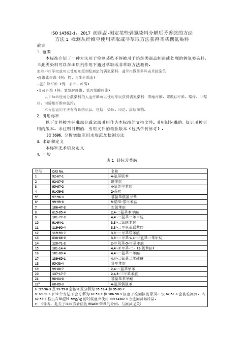
ISO14362-1：2017纺织品-测定某些偶氮染料分解后芳香胺的方法方法1检测从纤维中使用萃取或非萃取方法获得某些偶氮染料前言1.范围本标准介绍了一种方法用于检测某些不得被用于纺织类商品制造或处理的偶氮类染料，且此类染料可以在还原剂作用下通过萃取或非萃取方法测得。

那些不用萃取就可以使用还原剂检测出的偶氮染料，通常用做颜料料或直接染色-纤维素纤维（例：棉、再生纤维素）--蛋白质纤维（例：羊毛、丝绸）-合成纤维（例：聚酰胺纤维、聚丙烯酸纤维）以下这些使用分散染料的人造纤维可以使用萃取获得偶氮染料：聚酯纤维、聚酰胺纤维、醋纤、三醋纤、丙烯酸纤维和氯纶。

本方法适用于所有有色纺织品，包括：染色、印花、涂层织物。

2.引用标准以下文件被本标准部分或全部引用作为本标准的支持文件。

引用旧标准的，仅引用被引用的版本。

未注明日期的，引用文件的最新版本（包括任何修订）。

ISO3696,分析实验室用水规范及检测方法3.术语和定义本标准无术语及定义4.一般表1目标芳香胺序号CAS No.名称192-67-14-氨基联苯292-87-5联苯胺395-67-24-氯邻甲苯胺491-59-82-萘胺5a97-56-3邻氨基偶氮甲苯6a99-55-85-硝基-邻甲苯胺7106-47-8对氯苯胺8615-05-42,4-二氨基苯甲醚9101-77-94,4’-二氨基二苯甲烷1091-94-13,3’-二氯联苯胺11119-90-43,3’-二甲氧基联苯胺12119-93-73,3’-二甲基联苯胺13838-88-03,3’-二甲基-4,4’-二氨基二苯甲烷14120-71-82-甲氧基-5-甲基苯胺15101-14-44,4’-亚甲基-二-（2-氯苯胺）16101-80-44,4’-二氨基二苯醚17139-65-14,4’-二氨基二苯硫醚1895-53-4邻甲苯胺1995-80-72,4-二氨基甲苯20137-17-72,4,5-三甲基苯胺2190-04-0邻氨基苯甲醚22b60-09-34-氨基偶氮苯a:97-56-3及99-55-8会被还原分解为95-53-4和95-80-7b:60-09-3在这个方法下会分解为62-53-3和106-50-3.但由于检测限的原因，仅62-53-3会被检测到，当62-53-3检出含量超过5mg/kg的时候就应使用ISO14362.3方法测试该样品。

作业条件危险性分析LEC评价法

作业条件危险性分析LEC评价法LEC评价法(美国安全专家K.J.格雷厄姆和K.F.金尼提出)是对具有潜在危险性作业环境中的危险源进行半定量的安全评价方法。

LEC评价法(美国安全专家K.J.格雷厄姆和K.F.金尼提出)用于评价操作人员在具有潜在危险性环境中作业时的危险性、危害性。

该方法用与系统风险有关的三种因素指标值的乘积来评价操作人员伤亡风险大小，这三种因素分别是：L（likelihood，事故发生的可能性）、E（exposure，人员暴露于危险环境中的频繁程度）和C（consequence，一旦发生事故可能造成的后果）。

给三种因素的不同等级分别确定不同的分值，再以三个分值的乘积D（danger，危险性）来评价作业条件危险性的大小，即：D=L×E×C风险分值D=LEC。

D值越大，说明该系统危险性大，需要增加安全措施，或改变发生事故的可能性，或减少人体暴露于危险环境中的频繁程度，或减轻事故损失，直至调整到允许范围内。

一、量化分值标准对这3种方面分别进行客观的科学计算，得到准确的数据，是相当繁琐的过程。

为了简化评价过程，采取半定量计值法。

即根据以往的经验和估计，分别对这3方面划分不同的等级，并赋值。

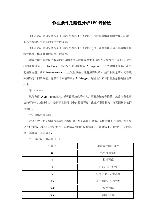
具体如下：二、事故发生的可能性（L）三、暴露于危险环境的频繁程度（E）四、发生事故产生的后果（C）五、风险分析根据公式：风险D=LEC就可以计算作业的危险程度，并判断评价危险性的大小。

其中的关键还是如何确定各个分值，以及对乘积值的分析、评价和利用。

根据经验，总分在20以下是被认为低危险的，这样的危险比日常生活中骑自行车去上班还要安全些；如果危险分值到达70～160之间，那就有显著的危险性，需要及时整改；如果危险分值在160～320之间，那么这是一种必须立即采取措施进行整改的高度危险环境；分值在320以上的高分值表示环境非常危险，应立即停止生产直到环境得到改善为止。

值得注意的是，LEC风险评价法对危险等级的划分，一定程度上凭经验判断，应用时需要考虑其局限性，根据实际情况予以修正。

Testing Fisher, Neyman, Pearson, and Bayes

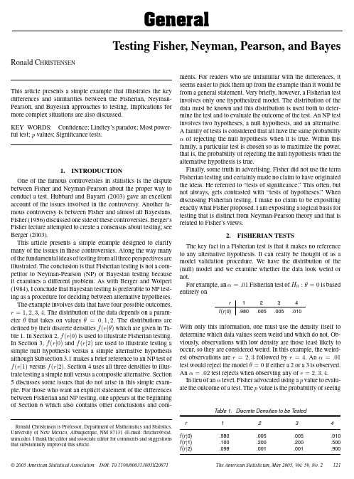
GeneralTesting Fisher,Neyman,Pearson,and Bayes Ronald C HRISTENSENThis article presents a simple example that illustrates the keydifferences and similarities between the Fisherian,Neyman-Pearson,and Bayesian approaches to testing.Implications formore complex situations are also discussed.KEY WORDS:Conﬁdence;Lindley’s paradox;Most power-ful test;p values;Signiﬁcance tests.1.INTRODUCTIONOne of the famous controversies in statistics is the disputebetween Fisher and Neyman-Pearson about the proper way toconduct a test.Hubbard and Bayarri(2003)gave an excellentaccount of the issues involved in the controversy.Another fa-mous controversy is between Fisher and almost all Bayesians.Fisher(1956)discussed one side of these controversies.Berger’sFisher lecture attempted to create a consensus about testing;seeBerger(2003).This article presents a simple example designed to clarifymany of the issues in these controversies.Along the way manyof the fundamental ideas of testing from all three perspectives areillustrated.The conclusion is that Fisherian testing is not a com-petitor to Neyman-Pearson(NP)or Bayesian testing becauseit examines a different problem.As with Berger and Wolpert(1984),I conclude that Bayesian testing is preferable to NP test-ing as a procedure for deciding between alternative hypotheses.The example involves data that have four possible outcomes, r=1,2,3,4.The distribution of the data depends on a param-eterθthat takes on valuesθ=0,1,2.The distributions aredeﬁned by their discrete densities f(r|θ)which are given in Ta-ble1.In Section2,f(r|0)is used to illustrate Fisherian testing.In Section3,f(r|0)and f(r|2)are used to illustrate testing asimple null hypothesis versus a simple alternative hypothesisalthough Subsection3.1makes a brief reference to an NP test of f(r|1)versus f(r|2).Section4uses all three densities to illus-trate testing a simple null versus a composite alternative.Section 5discusses some issues that do not arise in this simple exam-ple.For those who want an explicit statement of the differences between Fisherian and NP testing,one appears at the beginning of Section6which also contains other conclusions and com-Ronald Christensen is Professor,Department of Mathematics and Statistics, University of New Mexico,Albuquerque,NM87131(E-mail:ﬂetcher@stat. ).I thank the editor and associate editor for comments and suggestions that substantially improved this article.ments.For readers who are unfamiliar with the differences,it seems easier to pick them up from the example than it would be from a general statement.Very brieﬂy,however,a Fisherian test involves only one hypothesized model.The distribution of the data must be known and this distribution is used both to deter-mine the test and to evaluate the outcome of the test.An NP test involves two hypotheses,a null hypothesis,and an alternative.A family of tests is considered that all have the same probability αof rejecting the null hypothesis when it is true.Within this family,a particular test is chosen so as to maximize the power, that is,the probability of rejecting the null hypothesis when the alternative hypothesis is true.Finally,some truth in advertising.Fisher did not use the term Fisherian testing and certainly made no claim to have originated the ideas.He referred to“tests of signiﬁcance.”This often,but not always,gets contrasted with“tests of hypotheses.”When discussing Fisherian testing,I make no claim to be expositing exactly what Fisher proposed.I am expositing a logical basis for testing that is distinct from Neyman-Pearson theory and that is related to Fisher’s views.2.FISHERIAN TESTSThe key fact in a Fisherian test is that it makes no reference to any alternative hypothesis.It can really be thought of as a model validation procedure.We have the distribution of the (null)model and we examine whether the data look weird or not.For example,anα=.01Fisherian test of H0:θ=0is based entirely onr1234f(r|0).980.005.005.010With only this information,one must use the density itself to determine which data values seem weird and which do not.Ob-viously,observations with low density are those least likely to occur,so they are considered weird.In this example,the weird-est observations are r=2,3followed by r=4.Anα=.01 test would reject the modelθ=0if either a2or a3is observed. Anα=.02test rejects when observing any of r=2,3,4.In lieu of anαlevel,Fisher advocated using a p value to evalu-ate the outcome of a test.The p value is the probability of seeingT able1.Discrete Densities to be T estedr1234f(r|0).980.005.005.010 f(r|1).100.200.200.500 f(r|2).098.001.001.900©2005American Statistical Association DOI:10.1198/000313005X20871The American Statistician,May2005,Vol.59,No.2121something as weird or weirder than you actually saw.(There isno need to specify that it is computed under the null hypothe-sis because there is only one hypothesis.)In this example,theweirdest observations are2and3and they are equally weird.Their combined probability is.01which is the p value regardlessof which you actually observe.If you see a4,both2and3areweirder,so the combined probability is.02.r1234f(r|0).980.005.005.010p value 1.00.01.01.02In Fisherian testing,the p value is actually a more fundamentalconcept than theαlevel.Technically,anαlevel is simply adecision rule as to which p values will cause one to reject thenull hypothesis.In other words,it is merely a decision point asto how weird the data must be before rejecting the null model.If the p value is less than or equal toα,the null is rejected.Implicitly,anαlevel determines what data would cause one toreject H0and what data will not cause rejection.Theαlevelrejection region is deﬁned as the set of all data points that havea p value less than or equal toα.Note that in this example,anα=.01test is identical to anα=.0125test.Both rejectwhen observing either r=2or3.Moreover,the probability ofrejecting anα=.0125test when the null hypothesis is true isnot.0125,it is.01.However,Fisherian testing is not interested in what the probability of rejecting the null hypothesis will be,it is interested in what the probability was of seeing weird data.The philosophical basis of a Fisherian test is akin to proof bycontradiction.We have a model and we examine the extent towhich the data contradict the model.The basis for suggesting acontradiction is actually observing data that are highly improb-able under the model.The p value gives an excellent measure ofthe extent to which the data do not contradict the model.(Large p values do not contradict the model.)If anαlevel is chosen, for any semblance of a contradiction to occur,theαlevel mustbe small.On the other hand,even without a speciﬁc alternative,makingαtoo small will defeat the purpose of the test,making itextremely difﬁcult to reject the test for any reason.A reasonableview would be that anαlevel should never be chosen;that ascientist should simply evaluate the evidence embodied in the pvalue.As in any proof by contradiction,the results are skewed.Ifthe data contradict the model,we have evidence that the modelis invalid.If the data do not contradict the model,we have anattempt at proof by contradiction in which we got no contradic-tion.If the model is not rejected,the best one can say is that thedata are consistent with the model.Not rejecting certainly doesnot prove that the model is correct,whence comes the commonexhortation that one should never accept a null hypothesis.3.SIMPLE VERSUS SIMPLE Consider testing the simple null hypothesis H0:θ=0versus the simple alternative hypothesis H A:θ=2.This now appears to be a decision problem.We have two alternatives and we are deciding between them.This formulation as a decision problem is a primary reason that Fisher objected to NP testing,see Fisher (1956,chap.4).The relevant information for this testing problem isr1234f(r|0).980.005.005.010f(r|2).098.001.001.900Before examining formal testing procedures,look at the dis-tributions.Intuitively,if we see r=4we are inclined to believe θ=2,if we see r=1we are quite inclined to believe that θ=0,and if we see either a2or a3,it is stillﬁve times morelikely that the data came fromθ=0.Although Fisherian testing does not use an explicit alternative, there is nothing to stop us from doing two Fisherian tests:a test of H0:θ=0and then another test of H0:θ=2.The Fisherian tests both give perfectly reasonable results.The test for H0:θ=0has small p values for any of r=2,3,4.These are all strange values whenθ=0.The test for H0:θ=2has small p values when r=2,3.When r=4,we do not reject θ=2;when r=1,we do not rejectθ=0;when r=2,3,we reject bothθ=0andθ=2.The Fisherian tests are not being forced to choose between the two distributions.Seeing either a 2or a3is weird under both distributions.3.1Neyman-Pearson TestsNP tests treat the two hypotheses in fundamentally different ways.A test of H0:θ=0versus H A:θ=2is typically different from a test of H0:θ=2versus H A:θ=0.We examine the test of H0:θ=0versus H A:θ=2.NP theory seeks toﬁnd the bestαlevel test.αis the probability of rejecting H0when it is true.The rejection region is the set of data values that cause one to reject the null hypothesis,so under H0the probability of the rejection region must beα.The best test is deﬁned as the one with the highest power,that is, the highest probability of rejecting H0(observing data in the rejection region)when H A is true.Deﬁning theαlevel as the probability of rejecting the null hypothesis when it is true places an emphasis on repeated sam-pling so that the Law of Large Numbers suggests that aboutαof the time you will make an incorrect decision,provided the null hypothesis is true in all of the samples.Although this is obviously a reasonable deﬁnition prior to seeing the data,its relevance after seeing the data is questionable.To allow arbitraryαlevels,one must consider randomized tests.A randomized test requires a randomized rejection region. How would one perform anα=.0125test?Three distinct tests are:(a)reject whenever r=4andﬂip a coin,if it comes up heads,reject when r=2;(b)reject whenever r=4andﬂip a coin,if it comes up heads,reject when r=3;(c)reject whenever r=2or3andﬂip a coin twice,if both come up heads,reject when r=4.It is difﬁcult to convince anyone that these are reasonable practical procedures.r1234f(r|0).980.005.005.010f(r|2).098.001.001.900f(r|2)/f(r|0).1.2.290As demonstrated in the famous Neyman-Pearson lemma(see Lehmann1997,chap.3),optimal NP tests are based on the likeli-hood ratio f(r|2)/f(r|0).The best NP test rejects for the largest values of the likelihood ratio,thus theα=.01NP test rejects122Generalwhen r=4.This is completely different from the Fisherian.01test of H0that rejected when r=2,3.(On the other hand,the α=.02NP test coincides with the Fisherian test.Both reject when observing any of r=2,3,4.)The power of theα=.01NP test is.9whereas the power of the Fisherianα=.01test isonly.001+.001=.002.Clearly the Fisherian test is not a goodway to decide between these alternatives.But then the Fishe-rian test was not designed to decide between two alternatives.Itwas designed to see whether the null model seemed reasonableand,on its own terms,it works well.Although the meaning of αdiffers between Fisherian and NP tests,we have chosen two examples,α=.01andα=.02,in which the Fisherian test(rejection region)also happens to deﬁne an NP test with thesame numerical value ofα.Such a comparison would not beappropriate if we had examined,say,α=.0125Fisherian andNP tests.NP testing and Fisherian testing are not comparable proce-dures,a point also made by Hubbard and Bayarri(2003).NPtesting is designed to optimally detect some alternative hypoth-esis and Fisherian testing makes no reference to any alternativehypothesis.I might suggest that NP testers tend to want to havetheir cake and eat it too.By this I mean that many of them wantto adopt the philosophy of Fisherian testing(involving p val-ues,using smallαlevels,and never accepting a null hypothesis)while still basing their procedure on an alternative hypothesis. In particular,the motivation for using smallαlevels seems tobe based entirely on the philosophical idea of proof by contra-ing a largeαlevel would eliminate the suggestion thatthe data are unusual and thus tend to contradict H0.However,NP testing cannot appeal to the idea of proof by contradiction.For example,in testing H0:θ=1versus H A:θ=2,the most powerful NP test would reject for r=4,even though r=4isthe most probable value for the data under the null hypothesis.(For anyα<.5,a randomized test is needed.)In particular,this example makes it clear that p values can have no role in NPtesting!See also Hubbard and Bayarri(2003)and discussion. It seems that once you base the test on wanting a large proba-bility of rejecting the alternative hypothesis,you have put your-self in the business of deciding between the two hypotheses. Even on this basis,the NP test does not always perform very well.The rejection region for theα=.02NP test of H0:θ=0 versus H A:θ=2includes r=2,3,even though2and3 areﬁve times more likely under the null hypothesis than under the alternative.Admittedly,2and3are weird things to see un-der either hypothesis,but when deciding between these speciﬁc alternatives,rejectingθ=0(acceptingθ=2)for r=2orT able2.Posterior Probabilities ofθ=0,2for T wo Prior Dis-tributions a and bPrior r1234f(r|0).980.005.005.010f(r|2).098.001.001.900p a(0)=1/2p a(0|r).91.83.83.01 p a(2)=1/2p a(2|r).09.17.17.99p b(0)=1/6p b(0|r).67.50.50.002 p b(2)=5/6p b(2|r).33.50.50.9983does not seem reasonable.The Bayesian approach to testing, discussed in the next subsection,seems to handle this decision problem well.3.2Bayesian TestsBayesian analysis requires us to have prior probabilities on the values ofθ.It then uses Bayes’theorem to combine the prior probabilities with the information in the data toﬁnd“posterior”probabilities forθgiven the data.All decisions aboutθare based entirely upon these posterior probabilities.The information in the data is obtained from the likelihood function.For an observed data value,say r=r∗,the likelihood is the function ofθdeﬁned by f(r∗|θ).In our simple versus simple testing example,let the prior prob-abilities onθ=0,2be p(0)and p(2).Applying Bayes’theorem to observed data r,we turn these prior probabilities into poste-rior probabilities forθgiven r,say p(0|r)and p(2|r).To do this we need the likelihood function which here takes on only the two values f(r|0)and f(r|2).From Bayes’theorem,p(θ|r)=f(r|θ)p(θ)f(r|0)p(0)+f(r|2)p(2),θ=0,2.Decisions are based on these posterior probabilities.Other things being equal,whichever value ofθhas the larger posterior prob-ability is the value ofθthat we will accept.If both posterior probabilities are near.5,we might admit that we do not know which is right.In practice,posterior probabilities are computed only for the value of r that was actually observed,but Table2gives posterior probabilities for all values of r and two sets of prior probabilities: (a)one in which each value ofθhas the same probability,1/2, and(b)one set in whichθ=2isﬁve times more probable than θ=0.As is intuitively reasonable,regardless of the prior distribu-tion,if you see r=4the posterior is heavily in favor ofθ=2, and if you see r=1the posterior substantially favorsθ=0. The key point is what happens when r equals2or3.With equal prior weight on theθ’s,the posterior heavily favorsθ=0, that is,with r=2,p a(0|2)=.83,p a(2|2)=.17,and with r=3,p a(0|3)=.83,p a(2|3)=.17.It is not until our prior makesθ=2ﬁve times more probable thanθ=0that we wash out the evidence from the data thatθ=0is more likely,that is, p b(0|2)=p b(2|2)=.50and p b(0|3)=p b(2|3)=.50.Given the prior,the Bayesian procedure is always reasonable.The Bayesian analysis gives no special role to the null hy-pothesis.It treats the two hypotheses on an equal footing.That NP theory treats the hypotheses in fundamentally different ways is something that many Bayesiansﬁnd disturbing.If utilities are available,the Bayesian can base a decision on maximizing expected posterior utility.Berry(2004)discussed the practical importance of developing approximate utilities for designing clinical trials.The absence of a clear source for the prior probabilities seems to be the primary objection to the Bayesian procedure.Typically, if we have enough data,the prior probabilities are not going to matter because the posterior probabilities will be substantially the same for different priors.If we do not have enough data,the posteriors will not agree but why should we expect them to?The best we can ever hope to achieve is that reasonable people(with The American Statistician,May2005,Vol.59,No.2123reasonable priors)will arrive at a consensus when enough data are collected.In the example,seeing one observation of r=1 or4is already enough data to cause substantial consensus.One observation that turns out to be a2or a3leaves us wanting more data.4.SIMPLE VERSUS COMPOSITENow consider testing the simple null hypothesis H0:θ=0 versus the composite alternative hypothesis H A:θ>0.Of course the composite alternative has only two values.Looking at the distributions in Table1,the intuitive conclusions are pretty clear.For r=1,go withθ=0.For r=4,go withθ=2.For r=2,3,go withθ=1.Fisherian testing has nothing new to add to this situation ex-cept the observation that whenθ=1,none of the data are really weird.In this case,the strangest observation is r=1which has a p value of.1.The best thing that can happen in NP testing of a composite alternative is to have a uniformly most powerful test.With H A:θ>0,letθ∗be a particular value that is greater than0.Test the simple null H0:θ=0against the simple alternative H A:θ=θ∗.If,for a givenα,the most powerful test has the same rejection region regardless of the value ofθ∗,then that test is the uniformly most powerful test.It is a simple matter to see that theα=.01 NP most powerful test of H0:θ=0versus H A:θ=1rejects when r=4.Because the most powerful tests of the alternatives H A:θ=1and H A:θ=2are identical,and these are the only permissible values ofθ>0,this is the uniformly most powerful α=.01test.The test makes a“bad”decision when r=2,3 because withθ=1as a consideration,you would intuitively like to reject the test.Theα=.02uniformly most powerful test rejects for r=2,3,4,which is in line with our intuitive evaluation,but recall from the previous section that this is the test that(intuitively)should not have rejected for r=2,3when testing only H A:θ=2.An even-handed Bayesian approach might take prior proba-bilities that are the same for the null hypothesis and the alter-native,that is,Pr[θ=0]=.5and Pr[θ>0]=.5.Moreover, we might then put the same prior weight on every possibleθvalue within the alternative,thus Pr[θ=1|θ>0]=.5and Pr[θ=2|θ>0]=.5.Equivalently,p(0)=.5,p(1)=.25,and p(2)=.25.The posterior probabilities arer1234p(0|r).908.047.047.014p(1|r).046.948.948.352p(2|r).045.005.005.634Pr[θ>0|r].091.953.953.986These agree well with the intuitive conclusions,even though the prior puts twice as much weight onθ=0as on the otherθ’s. The Bayesian approach to testing a simple null against a com-posite alternative can be recast as testing a simple null versus a simple ing the prior probability on the values ofθgiven that the alternative hypothesis is true,one canﬁnd the average distribution for the data under the alternative.With Pr[θ=1|θ>0]=.5and Pr[θ=2|θ>0]=.5,the av-erage distribution under the alternative is.5f(r|1)+.5f(r|2). The Bayesian test of theθ=0density f(r|0)against this aver-age density for the data under the alternative yields the posterior probabilities p(0|r)and Pr[θ>0|r].It might also be reasonable to put equal probabilities on ev-eryθvalue.In decision problems like this,where you know the(sampling)distributions,the only way to get unreasonable Bayesian answers is to use an unreasonable prior.5.GENERAL MATTERS5.1Fisherian TestingOne thing that the example in Section2does not illustrate is that in a Fisherian test,it is not clear what aspect of the model is being rejected.If y1,y2,...,y n are independent N(µ,σ2)and we perform a t test of H0:µ=0,a rejection could mean thatµ=0,or it could mean that the data are not independent,or it could mean that the data are not normal,or it could mean that the variances of the observations are not equal.In other words, rejecting a Fisherian test suggests that something is wrong with the model.It does not specify what is wrong.The example of a t test raises yet another question.Why should we summarize these data by looking at the t statistic,y−0s/√n?One reason is purely practical.In order to perform a test,one must have a known distribution to compare to the data.Without a known distribution there is no way to identify which values of the data are weird.With the normal data,even when assuming µ=0,we do not knowσ2so we do not know the distribution of the data.By summarizing the data into the t statistic,we get a function of the data that has a known distribution,which allows us to perform a test.Another reason is essentially:why not look at the t statistic?If you have another statistic you want to base a test on,the Fisherian tester is happy to oblige.To quote Fisher(1956,p.49),the hypothesis should be rejected“if any relevant feature of the observational record can be shown to[be] sufﬁciently rare.”After all,if the null model is correct,it should be able to withstand any challenge.Moreover,there is no hint in this passage of worrying about the effects of performing multiple tests.Inﬂating the probability of Type I error(rejecting the null when it is true)by performing multiple tests is not a concern in Fisherian testing because the probability of Type I error is not a concern in Fisherian testing.The one place that possible alternative hypotheses arise in Fisherian testing is in the choice of test statistics.Again quoting Fisher(1956,p.50),“In choosing the grounds upon which a general hypothesis should be rejected,personal judgement may and should properly be exercised.The experimenter will rightly consider all points on which,in the light of current knowledge, the hypothesis may be imperfectly accurate,and will select tests, so far as possible,sensitive to these possible faults,rather than to others.”Nevertheless,the logic of Fisherian testing in no way depends on the source of the test statistic.There are twoﬁnal points to make on how this approach to testing impacts standard data analysis.First,F tests andχ2tests are typically rejected only for large values of the test statistic.Clearly,in Fisherian testing,that is inappropriate.Finding the p value for an F test should involve ﬁnding the density associated with the observed F statistic and124Generalﬁnding the probability of getting any value with a lower density.This will be a two-tailed test,rejecting for values that are very large or very close to 0.As a practical matter,it is probably sufﬁcient to always remember that “one-sided p values”very close to 1should make us as suspicious of the model as one-sided p values near 0.Christensen (2003)discusses situations that cause F statistics to get close to 0.Second,although Fisher never gave up on his idea of ﬁducial inference,one can use Fisherian testing to arrive at “conﬁdence regions”that do not involve either ﬁducial inference or repeated sampling.A (1−α)conﬁdence region can be deﬁned simply as a collection of parameter values that would not be rejected by a Fisherian αlevel test,that is,a collection of parameter values that are consistent with the data as judged by an αlevel test.This deﬁnition involves no long run frequency interpreta-tion of “conﬁdence.”It makes no reference to what proportion of hypothetical conﬁdence regions would include the true pa-rameter.It does,however,require one to be willing to perform an inﬁnite number of tests without worrying about their fre-quency interpretation.This approach also raises some curious ideas.For example,with the normal data discussed earlier,this leads to standard t conﬁdence intervals for µand χ2conﬁdence intervals for σ2,but one could also form a joint 95%conﬁdence region for µand σ2by taking all the pairs of values that satisfy|y −µ|σ/√n<1.96.Certainly all such µ,σ2pairs are consistent with the data as summarized by ¯y .5.2Neyman-Pearson TestsTo handle more general testing situations,NP theory has de-veloped a variety of concepts such as unbiased tests,invariant tests,and αsimilar tests;see Lehmann (1997).For example,the two-sided t test is not a uniformly most powerful test but it is a uniformly most powerful unbiased test.Similarly,the standard F test in regression and analysis of variance is a uniformly most powerful invariant test.The NP approach to ﬁnding conﬁdence regions is also to ﬁnd parameter values that would not be rejected by a αlevel test.However,just as NP theory interprets the size αof a test as the long run frequency of rejecting an incorrect null hypothesis,NP theory interprets the conﬁdence 1−αas the long run probability of these regions including the true parameter.The rub is that you only have one of the regions,not a long run of them,and you are trying to say something about this parameter based on these data.In practice,the long run frequency of αsomehow gets turned into something called “conﬁdence”that this parameter is within this particular region.Although I admit that the term “conﬁdence,”as commonly used,feels good,I have no idea what “conﬁdence”really means as applied to the region at hand.Hubbard and Bayarri (2003)made a case,implicitly,that an NP concept of conﬁdence would have no meaning as applied to the region at hand,that it only applies to a long run of similar intervals.Students,almost invari-ably,interpret conﬁdence as posterior probability.For example,if we were to ﬂip a coin many times,about half of the time wewould get heads.If I ﬂip a coin and look at it but do not tell you the result,you may feel comfortable saying that the chance of heads is still .5even though I know whether it is heads or tails.Somehow the probability of what is going to happen in the future is turning into conﬁdence about what has already hap-pened but is unobserved.Since I do not understand how this transition from probability to conﬁdence is made (unless one is a Bayesian in which case conﬁdence actually is probability),I do not understand “conﬁdence.”5.3Bayesian TestingBayesian tests can go seriously wrong if you pick inappro-priate prior distributions.This is the case in Lindley’s famous paradox in which,for a seemingly simple and reasonable testing situation involving normal data,the null hypothesis is accepted no matter how weird the observed data are relative to the null hy-pothesis.The datum is X |µ∼N (µ,1).The test is H 0:µ=0versus H A :µ>0.The priors on the hypotheses do not re-ally matter,but take Pr[µ=0]=.5and Pr[µ>0]=.5.In an attempt to use a noninformative prior,take the density of µgiven µ>0to be ﬂat on the half line.(This is an improper prior but similar proper priors lead to similar results.)The Bayesian test compares the density of the data X under H 0:µ=0to the average density of the data under H A :µ>0.(The latter involves integrating the density of X |µtimes the density of µgiven µ>0.)The average density under the alternative makes any X you could possibly see inﬁnitely more probable to have come from the null distribution than from the alternative.Thus,anything you could possibly see will cause you to accept µ=0.Attempting to have a noninformative prior on the half line leads one to a nonsensical prior that effectively puts all the probability on unreasonably large values of µso that,by comparison,µ=0always looks more reasonable.6.CONCLUSIONS AND COMMENTSThe basic elements of a Fisherian test are:(1)There is a prob-ability model for the data.(2)Multidimensional data are sum-marized into a test statistic that has a known distribution.(3)This known distribution provides a ranking of the “weirdness”of various observations.(4)The p value,which is the probability of observing something as weird or weirder than was actually observed,is used to quantify the evidence against the null hy-pothesis.(5)αlevel tests are deﬁned by reference to the p value.The basic elements of an NP test are:(1)There are two hy-pothesized models for the data:H 0and H A .(2)An αlevel is chosen which is to be the probability of rejecting H 0when H 0is true.(3)A rejection region is chosen so that the probability of data falling into the rejection region is αwhen H 0is true.With discrete data,this often requires the speciﬁcation of a random-ized rejection region in which certain data values are randomly assigned to be in or out of the rejection region.(4)Various tests are evaluated based on their power properties.Ideally,one wants the most powerful test.(5)In complicated problems,properties such as unbiasedness or invariance are used to restrict the class of tests prior to choosing a test with good power properties.Fisherian testing seems to be a reasonable approach to model validation.In fact,Box (1980)suggested Fisherian tests,based on the marginal distribution of the data,as a method for validat-ing Bayesian models.Fisherian testing is philosophically basedThe American Statistician,May 2005,Vol.59,No.2125。

100618003磨合数据

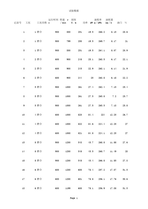
油门　％记录号工况工况名称运行时间　s转速　r∕mi扭矩　N．m功率　kW油耗率　g∕油耗量　kg∕11磨合90080023119.3265.2 5.1320.6 21磨合90079923019.3269.7 5.1721 31磨合90080023119.3264.1 5.0720.9 42磨合60090024523.1268.3 6.1722.1 52磨合60090024322.9268.1 6.1421.9 62磨合60090024423268.5 6.1522.2 73磨合900100026127.4262.47.1323.4 83磨合900100026127.3263.57.223.7 93磨合900100026127.3263.37.1823.5 104磨合600100052054.422412.2326.7 114磨合600100052254.6224.412.2327 124磨合600100052154.5224.112.2327 135磨合900120034843.7265.511.5527.6 145磨合900120034543.3265.711.4928 155磨合900120034543.4266.511.5327.8 166磨合600120060075.4237.217.8731.3 176磨合600120060175.5236.117.7630.6 186磨合600119960075.1236.917.8531.3 197磨合900140043063264.116.6432 207磨合900139843062.9263.716.6132.1 217磨合900140043063.1263.316.6132.5 228磨合6001399690101.1236.823.9837.4 238磨合6001398690101.3236.723.9537.1 248磨合6001400690101.1236.223.8837.1 259磨合6001600700117.3241.328.3443.3 269磨合6001601700117.6241.828.3343.3 279磨合6001600700117.2241.828.3343.5 289磨合6001601700117.2241.928.3643.8 299磨合6001600700117.5239.128.0542.8 309磨合6001597700116.8240.628.1642.8 3110磨合60015981030172.3224.938.8749.3 3210磨合60015981030172.7224.238.6949.7 3310磨合60015981030172.4224.938.7849.8 3410磨合60016011030172.8224.438.8249.6 3510磨合60016021030172.7225.738.8949.8 3610磨合60015981030172.4224.638.850.3 3710磨合60016011030172.6224.938.8350 3810磨合60016021030172.5225.738.9549.7 3910磨合60016021030172.8225.538.9450.1 4011磨合6001800861162.523538.0754 4111磨合6001800861162.4234.938.0754.1 4211磨合6001805860162235.237.9953.7 4311磨合6001795859161.8234.738.0353.9 4411磨合6001793859161.3234.838.0254.7 4511磨合6001805860162.123538.0154.2 4611磨合6001799860162233.938.0754.5 4711磨合6001801860162.3235.138.1152.4 4811磨合6001803860162.2233.337.8152.3 4911磨合6001798860162.623437.9353.1 5011磨合600180086016223437.9452.7 5111磨合6001799860162233.737.9453 5212磨合60017931200225.4225.951.0961 5312磨合60017961200225.9225.151.0660.6 5412磨合60018001200226.2225.551.0560.35512磨合60018011200226.5225.951.1260.6 5612磨合60018001200226225.450.9560.6 5712磨合60018001200225.9226.451.0660.9 5812磨合60017981200225.9225.851.0561 5912磨合60018021200227.3226.251.0460.9 6012磨合60018001200226.422651.1161.6 6112磨合60017991200225.7224.65161.1 6212磨合60018001200225.7225.551.0761 6312磨合60017951200225.5225.951.1361.4 6412磨合60018001200226.1225.851.0660.8 6512磨合60017981200225.8226.551.1961.1 6612磨合60018001200226.722651.1260.9 6713磨合60019051030205.5227.446.7860 6813磨合60019011030205.422846.7460.5 6913磨合60018961029204.4227.446.6661.2 7013磨合60019021030205.3227.446.7760.4 7113磨合60019021030205228.246.7861.2 7213磨合60019001030205.5228.146.7660.8 7313磨合60018971030205.8227.746.761.1 7413磨合60019021031206.5228.346.6960.9 7513磨合60018901030203.4229.646.7661.5 7613磨合60019001030205.9227.146.7261.2 7713磨合60018841029204.7228.846.7361.9 7813磨合60018961030204.2228.646.8560.9 7914磨合60018991300258.9223.558.0465.6 8014磨合60018981301258.3224.157.9966.5 8114磨合60019131305261.4222.557.9866.1 8214磨合60018981300258.1223.857.9466.1 8314磨合60018961301259.5224.157.8766.2 8414磨合60018921298257.6222.957.7666.3 8514磨合60019011300257.5223.257.765.9 8614磨合60019051302260.2223.857.7965.7 8714磨合60018971301261224.157.7165.9 8814磨合60019081302259222.257.7165.5 8914磨合60018991301258.3222.457.5163.8 9014磨合60018971300258.2222.557.4764.3 9114磨合60019021300257.9223.157.7764.1 9214磨合60019041299258.6222.657.6364.7 9314磨合60018961301258222.857.6365.2 9415磨合6001499700109.7238.126.0340.5 9515磨合6001500700109.9238.426.240.4 9615磨合6001499700109.9238.826.2340.3 9715磨合6001497700110238.326.1939.9 9815磨合6001499700109.9238.726.240.1 9915磨合6001498700109.9238.225.8340 10015磨合6001499700109.8238.726.2140.4 10115磨合6001501700110.1238.126.1740.2 10215磨合6001499700110.1237.526.1140.2 10315磨合6001499700109.9237.826.0240.2 10415磨合6001502700110.2237.525.9940.1 10515磨合6001495700109.8237.225.8940.4 10616磨合60012971200162.9212.834.7444.3 10716磨合60012981200163211.234.4444 10816磨合60012991200163.4213.634.7944.6 10916磨合60012991200163.2213.434.6844.311016磨合60012961200162.9212.734.7244.4 11116磨合60012991200163.4212.234.6144.3 11216磨合60012951200162.6212.534.6344.6 11316磨合60012961200162.9210.734.3844.5 11416磨合60013011200163.3209.234.0744.3燃油温度　℃机油压力　k机油温度　℃大气压力　k环境温度　℃相对湿度　％中冷后温　℃中冷前压　k中冷后压　k中冷前温　℃3.5 5.542.233.538101.13728.534188.83.3 5.342.925.334.6101.238.328.734387.73.2 5.243.217.333101.239.428.733590.27.28.941.831.551.210131.227.944382.87.59.144.426.546.9101.132.928.339688.76.98.644.816.238.4101.236.128.539587.19.71148.420.433.410137.828.843489.19.511.249.818.131.1101.139.429430899.311.150.216.728.2101.140.729.241491.621.823.460.820.527101.24229.341290.621.823.461.722.924.8101.243.729.441190.821.523.16223.322.8101.345.129.440891.325.526.666.627.121.7101.346.329.6517912526.166.42820.7101.446.929.6508922526.265.82820101.447.329.652090.3495085.838.619.1101.448.229.748893.451.25283.841.937.9101.137.42949892.947.748.695.24725.7101.247.830.449192.450.350.285.34149101.136.829.659590.849.949.986.740.940.7101.240.23057792.149.549.687.241.634.3101.342.730.257492.380.680.4111.84631.5101.344.530.455194.180.379.7112.241.928.4101.44630.554794.579.479.2112.141.727.1101.547.230.654794.5989712743.425.6101.548.430.959696.398.897.3128.14324.3101.549.331.159296.798.597127.843.323.4101.65031.259396.697.496.4128.142.823.1101.650.331.259296.699.698121.142.653.110134.738.660994.39997.5123.342.845.610137.339.160295.1 132.1129.9146.841.939101.140.230.757997.4 129.8127.5149.842.629.510140.840.259095.7 128.2126.3151.442.72510144.243.257697.3 129.7127.6152.543.122.2101.146.944.357197.8 129.4127.6152.143.319.7101.249.333.557097.9 129127.215343.618.1101.351.138.356798.1 128.1126153.642.116.7101.452.63856698.2 127.5125.7153.743.115.6101.453.837.656498.4 128.8127154.343.614.6101.554.938.356298.4 122119.4153.542.414.2101.555.437.960599.5 123.2120.115342.514.1101.655.63860499.5 122119.3151.942.814.1101.655.738.160599.6 122.3119.8151.14313.9101.655.737.960299.7 123.3120.6150.243.113.6101.65637.960099.8 122119.7152.943.713.6101.656.43860299.8 123120.1151.842.613.7101.656.437.960099.8 127.2124.3138.442.743.4101.433.836.662396.3 127.8124.7140.742.836.7101.436.537.761597.8 127.1124.2141.442.732.2101.538.937.761098.3 127.7124.9142.843.128.8101.640.937.561098.8 126.9124.1143.54326.3101.742.737.760898.8 162.5158.9166.143.323.3101.84538.3591100.9 162158.5166.843.921101.94737.6589101.1 161157.7167.243.318.110249.337.9589101.2160.6156.9167.443.316.21025138.1588101.2 159.8156.3168.443.215102.152.338.6588101.2 159.7156167.942.614.5102.152.938.5586101.5 159.1155.5168.642.313.7102.253.938.2584101.6 160.3156.6167.942.813.3102.254.537.5583101.6 159.3155.8169.743.713.1102.254.937.8583101.6 157.7154.216943.312.6102.355.638.3584101.4 157.7154.1167.941.912.2102.356.137.6583101.4 159155.8168.242.511.9102.356.637.9582101.6 158.9155.216943.511.7102.456.838.2581101.6 158.7155.1167.143.311.1102.357.337.6580101.7 159.2155.7166.743.510.7102.45837.7580101.5 141.513816043.611102.457.538.1592101.7 142.4138.7159.843.711.7102.456.837.8592101.7 142.7139.4158.643.111.7102.456.438.1590101.7 141.9138.51594311.7102.356.138590101.7 142.1138.6159.443.111.6102.355.537.7590101.7 141.8138.2160.443.111.6102.355.338.1589101.8 140.7137.4159.142.811.6102.355.137.7590101.7 142.5139.1159.343.111.4102.35538.1590101.7 140.2136.8159.142.711.2102.355.237.8589101.7 139.8136.4160.743.211.5102.354.838.1590101.7 141.4137.9159.143.112.1102.354.637.5587101.7 141.5138159.643.112.2102.354.637.6589101.7 167.1162.9175.143.411.9102.35537.5577103.6 1671631754311.7102.355.538.2575103.8 167.5162.9175.543.211.4102.455.738.4576103.9 166.7162.6177.243.811.3102.455.937.5575103.8 167.3163.2175.844.411.1102.456.237.8577103.6 166.3162.3175.644.911102.456.538.3578103.5 165.8161.8176.444.710.9102.456.738579103.3 168.4163.9174.644.110.6102.456.937.6580103.3 165.2161.3176.243.910.8102.456.938.4578103.4 166161.9175.144.510.7102.456.938580103.3 165.8161.3164.842.431.1101.632.939.3604102.2 166161.6167.142.826.4101.736.138.8592103.7 166.6162.316943.223101.83937.1589104.6 167.4162.9170.243.219.6101.941.537.4588104.9 166.3161.7170.843.117.310243.837.5586105.1 88.187.2114.442.51510246.138.154597.3 87.987.411542.613.2102.147.238.154996.7 87.286.5115.342.512.3102.24837.954896.8 87.487.1114.74311.6102.248.837.854696.9 87.687.1115.14311.7102.349.537.754197.5 86.185.5113.642.511.1102.350.437.653498.4 88.187.1113.943.711.2102.350.637.355495.5 87.487.1114.744.210.9102.350.937.254596.7 87.58711544.310.8102.351.337.454396.8 86.885.9115.943.110.6102.351.23854396.8 86.786.1116.14210.2102.351.338.254397 85.885.3116.341.79.9102.352.138.354296.8 114.2113.5135.143.89.4102.35437.645298.4 113.3113134.643.88.7102.455.737.4438100.5 113.1113.3133.444.38.4102.557.137.845298 113113.2134.642.58102.558.137.845397.9112.1112135.342.77.6102.558.837.945297.7 112.2111.9134.743.27.6102.559.337.745397.9 111.6111.3135.143.37.2102.659.83844898.4 111.4111.9135.1437.1102.659.838.344399.2 112.1112.3135.242.7 6.9102.66038.644698.7排气背压　k进气负压　k记录时间进气温度　℃涡后温度　℃进水温度　℃出水温度　℃84.786.819537.30.7-0.12010-09-16 15:54:4879.280.419838.10.6-0.12010-09-16 16:09:4880.985.820038.20.7-0.12010-09-16 16:24:4940.258.520634.30.7-0.12010-09-17 09:39:25648121336.40.6-0.12010-09-17 09:49:2635.48121237.60.7-0.12010-09-17 10:16:4777.483.621938.21-0.12010-09-17 14:17:3078.381.922339.40.9-0.12010-09-17 14:32:3084.281.322440.11-0.12010-09-17 14:47:3045.581.532240.3 1.1-0.12010-09-17 14:57:30748332841.1 1.4-0.12010-09-17 15:07:3172.883.233041.4 1.5-0.12010-09-17 15:17:3156.581.629442 1.9-0.12010-09-17 15:32:3181.683.729441.6 1.7-0.12010-09-17 15:47:3138.580.829441.3 1.7-0.12010-09-17 16:02:3176.384.137542.8 2.5-0.12010-09-17 16:12:3177.98536540.6 2.3-0.12010-09-18 09:49:5135.381.738250.7 2.4-0.22010-09-19 16:13:0332.281.433342.6 2.7-0.42010-09-20 09:42:1134.881.533643 2.9-0.42010-09-20 09:57:1236.480.933643.73-0.32010-09-20 10:12:1244.778.338346.24-0.52010-09-20 10:22:1248.682.438046.5 4.1-0.52010-09-20 10:32:1250.382.537846.3 4.2-0.52010-09-20 10:42:1249.282.536448.4 5.8-0.92010-09-20 10:52:1259.383.236248.9 5.8-0.92010-09-20 11:02:1357.282.936048.2 6.2-0.82010-09-20 11:12:135882.936048.8 5.9-0.92010-09-20 11:22:1359.583.234043.86-12010-09-21 07:55:1850.382.634945.4 5.7-0.92010-09-21 08:05:1949.282.840247.38.5-1.32010-09-21 08:15:1955.182.839052.48.6-1.12010-09-21 13:55:5242.882.340454.38.4-1.12010-09-21 14:05:5246.982.441154.78.6-1.12010-09-21 14:15:5243.282.341455.58.6-1.32010-09-21 14:25:5244.682.341655.28.5-1.12010-09-21 14:35:5345.680.541555.98.3-12010-09-21 14:45:5347.982.541554.58.6-1.12010-09-21 14:55:5348.182.541655.98.4-12010-09-21 15:05:5358.683.238257.79.3-1.32010-09-21 15:15:5352.482.838057.59.5-1.32010-09-21 15:25:5352.582.837854.89.7-1.42010-09-21 15:35:545382.237855.49.7-1.22010-09-21 15:45:5456.482.837753.29.3-1.42010-09-21 15:55:5453.382.837856.69.6-1.42010-09-21 16:05:5453.382.837555.59.6-1.42010-09-21 16:15:5433.282.335742.89.9-1.62010-09-22 09:15:3736.782.436444.39.8-1.62010-09-22 09:25:3839.182.537145.69.5-1.42010-09-22 09:35:384182.537445.89.8-1.52010-09-22 09:45:3842.682.637646.19.5-1.52010-09-22 09:55:3843.382.843555.113.7-1.82010-09-22 10:05:3845.482.943749.513.7-1.92010-09-22 10:15:3844.182.74369413.6-1.72010-09-22 10:25:3942.581.443696.313.7-1.72010-09-22 10:35:3942.882.843552.313.7-1.82010-09-22 10:45:3943.582.943466.313.8-1.82010-09-22 10:55:39 43.882.943454.913.7-1.82010-09-22 11:05:39 4482.84336713.8-1.72010-09-22 11:15:40 44.18243451.813.7-1.92010-09-22 11:25:40 44.282.943349.513.6-1.82010-09-22 11:35:40 43.982.943148.213.5-1.82010-09-22 11:45:4043.782.943148.913.9-1.62010-09-22 11:55:4044.182.743349.813.7-1.82010-09-22 12:05:40 4481.643148.413.8-1.72010-09-22 12:15:41 44.382.943051.213.6-1.82010-09-22 12:25:41 41.582.739950.612.8-1.82010-09-22 12:35:41 41.282.739849.913-1.82010-09-22 12:45:41 4182.639749.712.9-1.72010-09-22 12:55:41 40.782.139848.712.9-1.82010-09-22 13:05:41 40.978.939952.413-1.72010-09-22 13:15:42 40.882.740052.812.7-1.82010-09-22 13:25:42 40.682.639949.312.8-1.72010-09-22 13:35:42 40.382.639949.413.1-1.92010-09-22 13:45:42 40.581.839949.312.7-1.82010-09-22 13:55:42 40.578.140151.712.8-1.82010-09-22 14:05:42 40.482.740049.512.9-1.82010-09-22 14:15:43 40.382.640151.312.7-1.72010-09-22 14:25:4342.582.94495216.5-2.12010-09-22 14:35:4343.882.844951.516.4-1.92010-09-22 14:45:4344.381.145053.417.1-2.22010-09-22 14:55:43 46.382.945154.116.1-2.22010-09-22 15:05:44 45.182.945051.516.6-2.12010-09-22 15:15:44 458345050.816.1-22010-09-22 15:25:44 45.182.945154.316.5-2.22010-09-22 15:35:44 45.381.744952.116.9-2.12010-09-22 15:45:44 49.183.345152.516.1-2.22010-09-22 15:55:44 45.682.945048.616.5-2.12010-09-22 16:05:45 5983.443340.416.9-2.32010-09-23 09:23:11 74.785.444242.916.7-2.22010-09-23 09:33:11 76.58544644.316.5-2.32010-09-23 09:43:11 76.4854494516.2-2.22010-09-23 09:53:12 76.38545147.916.2-2.12010-09-23 10:03:12 68.182.837343.45-0.62010-09-23 10:13:1270.183.237242.6 4.6-0.72010-09-23 10:23:1271.383.437243.2 5.2-0.62010-09-23 10:33:1272.883.537243.2 5.1-0.62010-09-23 10:43:13 77.183.937243.8 5.2-0.62010-09-23 10:53:13 8283.637043 5.2-0.62010-09-23 11:03:13 76.384.437143.6 4.9-0.72010-09-23 11:13:13 73.68437145.2 5.1-0.72010-09-23 11:23:13 73.483.937145.3 5.1-0.72010-09-23 11:33:1473.183.937044.45-0.62010-09-23 11:43:1474.284.237046.8 5.2-0.62010-09-23 11:53:14 72.983.536946.2 4.9-0.62010-09-23 12:03:14 78.984.445346.4 5.3-0.72010-09-23 12:13:14 83.284.245545.2 5.4-0.72010-09-23 12:23:15 61.782.745244.7 5.6-0.62010-09-23 12:33:15 69.583.945045.4 5.5-0.72010-09-23 12:43:1568.483.445045.6 5.6-0.62010-09-23 12:53:1569.483.645045.4 5.6-0.72010-09-23 13:03:15 74.58444945.7 5.5-0.72010-09-23 13:13:15 80.783.744846.3 5.6-0.72010-09-23 13:23:16 82.387.344746.7 5.6-0.72010-09-23 13:33:16。

LEC风险评价标准及风险确定准则

LEC风险评价标准及风险确定准则一、引言LEC（Lowest Effect Concentration）风险评价是一种常用的环境风险评价方法，用于确定化学物质对生物体的毒性效应。

本文将介绍LEC风险评价标准及风险确定准则，包括评价指标、评价方法和评价结果等内容。

二、评价指标1. LEC值：LEC值是评价化学物质对生物体的毒性效应的关键指标。

它表示在实验条件下，化学物质对生物体产生最低效应的浓度或剂量。

LEC值越低，说明化学物质对生物体的毒性效应越高。

2. 毒性分类：根据LEC值的大小，将化学物质分为无毒、低毒、中毒和高毒四个等级。

无毒表示LEC值大于100 mg/L；低毒表示LEC值介于10-100 mg/L；中毒表示LEC值介于1-10 mg/L；高毒表示LEC值小于1 mg/L。

三、评价方法1. 实验设计：LEC风险评价通常采用实验室实验方法进行。

首先，选择适当的生物体，如水生生物、昆虫或小型哺乳动物等，作为评价对象。

然后，根据评价的目的和要求，确定实验方案，包括化学物质的浓度梯度、实验时间和观察指标等。

2. 实验步骤：将评价对象暴露于不同浓度的化学物质溶液中，观察一定时间后，记录生物体的毒性效应，如死亡率、生长受抑制率或行为异常等。

根据实验结果，计算出LEC值。

3. 数据处理：通过统计学方法对实验数据进行处理，确定LEC值及其置信区间。

常用的方法包括Probit分析、Logit分析和线性回归分析等。

四、评价结果1. LEC值的解释：根据LEC值的大小，可以对化学物质的毒性进行解释。

LEC值越低，说明化学物质对生物体的毒性效应越高。

根据LEC值，可以将化学物质进行毒性分类，为环境风险评估提供参考依据。

2. 风险确定准则：根据LEC值和毒性分类，可以制定相应的风险确定准则。

例如，对于无毒化学物质，可以确定其在环境中的安全浓度；对于高毒化学物质，需要采取严格的管控措施，以防止对生物体和环境造成严重危害。

9-芴甲基-n-琥珀酰亚胺碳酸酯质量标准

9-芴甲基-n-琥珀酰亚胺碳酸酯（又称FMOC-Cl）是一种常用的化学试剂，在有机合成和蛋白质化学中具有广泛的应用。

它的质量标准是关键的，因为它直接影响到使用它的实验结果和最终产品的质量。

在本文中，我们将对FMOC-Cl的质量标准进行深入的评估和探讨，以便更好地理解和应用这一化合物。

我们需要了解FMOC-Cl的化学性质和用途。

FMOC-Cl是一种固体试剂，可以被用来保护氨基酸，从而在蛋白质合成和分析中发挥重要作用。

它的化学结构和纯度对实验结果有着至关重要的影响，因此质量标准必须严格把控。

在质量标准中，应明确规定其化学纯度、溶解度、熔点、红外光谱等关键指标，以确保产品的稳定性和可靠性。

我们需要深入了解FMOC-Cl的生产工艺和进行质量控制的关键环节。

在生产过程中，应严格按照国际通用的生产标准和流程进行操作，确保产品的稳定性和一致性。

应建立完善的质量控制体系，包括原料的采购、生产过程的监控、成品的检验等环节，以保证产品质量符合标准要求。

在质量标准的制定中，应考虑到FMOC-Cl在不同领域的应用需求，制定相应的质量标准。

在药物合成领域，对FMOC-Cl的纯度要求可能更高，因此质量标准应该更加严格；而在化学合成领域，对FMOC-Cl的溶解度和稳定性可能更为关键，因此质量标准中应侧重考虑这些指标。

质量标准应该是综合考虑应用需求和产品特性的结果，以保证产品的质量和可靠性。

在文章的总结部分，我们可以回顾本文对FMOC-Cl质量标准的深入评估，并得出结论。

FMOC-Cl作为一种重要的化学试剂，在有机合成和蛋白质化学中具有广泛的应用，其质量标准直接影响到实验结果和产品质量。

在制定质量标准时，应考虑到其化学性质、生产工艺和应用需求，以确保产品的稳定性和可靠性。

为了更好地理解和应用FMOC-Cl，我们需要不断深入研究其质量标准，并加强交流和合作，共同推动该领域的发展。

个人观点和理解：在实际操作中，对于化学试剂的质量标准要求应该更加严格，以确保实验结果的准确性和可靠性。

超高效液相色谱

超高效液相色谱‎超高效液相色谱‎【摘要】‎建立了同‎时测定玩具中16‎种致癌和致敏染料‎（酸性红2‎6、碱性红‎9、分散蓝‎1、酸性紫4‎9、分散蓝‎3、溶剂黄‎1、分散蓝10‎6、分散橙‎3、分散黄‎3、碱性紫‎1、碱性紫‎3、分散红‎1、溶剂黄‎3、分散蓝‎124、溶‎剂黄2、分‎散橙37）的超高‎效液相色谱-串联‎质谱分析方法。

纺‎织品、皮革、纸张‎、木材、气球、造‎型黏土、贴纸、可‎接触液体等不同类‎型的玩具材料经超‎声提取后，以wa‎t ers acq‎u ity upl‎c beh c1‎8色谱柱（50 ‎m m ×‎2.1 mm，‎ 1.7 μm‎）分离后进行up‎l c/ms/ms‎多反应监测模式下‎的定性及定量分析‎。

16种致癌和致‎敏染料的方法检出‎限为1.0‎~8.0 ‎μg/kg；在‎5~100 μg‎/kg范围内的低‎、中、高3个添加‎水平的平均回收率‎为81.3‎%～98.‎6%；日内精密‎度均小于11%，‎日间精密度均小于‎14%。

本方法准‎确、快速、灵敏度‎高，可用于玩具的‎实际检验工作。

‎‎【关键词】‎‎超高效液‎相色谱-串联质谱‎;玩具; 致癌‎染料; 致敏染料‎simulta‎n eous de‎t erminat‎i on of 1‎6carcin‎o genic a‎n d aller‎g enous d‎y estuffs‎in toys‎by ultr‎a perfor‎m ance li‎q uid chr‎o matogra‎p hy tand‎e m mass ‎s pectrom‎e tryma q‎i ang，bai‎hua*，wa‎n g chao，‎z hang qi‎n g，ma we‎i，zhou x‎i n，dong ‎y i-yang，‎w ang bao‎-lin(chi‎n ese aca‎d emy of ‎i nspecti‎o n and q‎u arantin‎e，beijin‎g100123‎)(china ‎a gricult‎u re univ‎e rsity，b‎e ijing1‎00083)(d‎o ngning ‎e ntry-ex‎i st insp‎e ction a‎n d quara‎n tine bu‎r eau，don‎g ning 15‎7200)abs‎t ract a ‎p rehensi‎v e analy‎t ical me‎t hod bas‎e d on ul‎t ra perf‎o rmance ‎l iquid c‎h romatog‎r aphy ta‎n dem mas‎sspectr‎o metry h‎a s been ‎d evelope‎d for th‎e simult‎a neousd‎e termina‎t ion of ‎16 carci‎n ogenic ‎a ndalle‎r genous ‎d yestuff‎s(acid r‎e d 26，ba‎s ic red ‎9，disper‎s e blue ‎1，acid v‎i olet 49‎，dispers‎e blue 3‎，solvent‎yellow ‎1，disper‎s ed blue‎106，dis‎p erse or‎a nge 3，d‎i sperse ‎y ellow 3‎，basic v‎i olet 1，‎b asic vi‎o let 3，d‎i sperse ‎r ed 1，so‎l vent ye‎l low 3，d‎i sperse ‎b lue 124‎，solvent‎yellow ‎2 and di‎s perse o‎r ange 37‎).variou‎s toysa‎m ples，in‎c luding ‎t extile，‎l eather，‎p aper，wo‎o d，ballo‎o n，model‎i ng clay‎，limitat‎i on tatt‎o o and a‎q ueous l‎i quid，we‎r e extra‎c ted und‎e r ultra‎s onicati‎o n.quali‎t ative a‎n dquant‎i tative ‎a nalysis‎was car‎r ied out‎for the‎analyte‎under t‎h e mrm m‎o de afte‎r the ch‎r omatogr‎a phic se‎p aration‎on wate‎r s acqui‎t y uplc ‎b eh c18(‎50 mm ×‎ 2.1 m‎m，1.7‎μm) col‎u mn.the ‎l imits o‎f quanti‎t ation(l‎o q) for ‎t he 16 d‎y estuffs‎were in‎the ran‎g e of‎1.0－‎8.0 μg/k‎g.the me‎a n recov‎e ries at‎the thr‎e e spike‎d levels‎of 5－10‎0μg/kg ‎w ere 8‎1.3%－9‎ 8.6%，w‎i th the ‎i ntra-da‎y precis‎i on less‎than 11‎% and th‎e inter-‎d ay prec‎i sion le‎s s than ‎14%.the ‎m ethod i‎s accura‎t e，rapid‎，sensiti‎v e，and a‎d apt to ‎t he insp‎e ction o‎f the 16‎dyestuf‎f s in to‎y s. keyw‎o rds ult‎r a perfo‎r mance l‎i quid ch‎r omatogr‎a phy tan‎d em mass‎spectro‎m etry; t‎o ys; car‎c inogeni‎c dyestu‎f fs; all‎e rgenous‎dyestuf‎f s 1 引言‎我国是玩具产品的‎生产和消费大国，‎也是国际玩具产品‎的主要出口国。

美国药典系统适宜性试验及注射用水的检测

制药用水是洁净度很高的水，在 TOC 测定中，适宜用 IC 前处理法（NPOC 法）。即先通过样品酸化及曝气去除 IC（无机
PeakProfile 2
1
碳），然后测量 NPOC（不可吹除有机碳）。在 TOC-V 操作软件中，建立标准曲线
模板，在界面上选择〖根据 USP/EP 建立标准曲线〗。使用此标准曲线模板作标准曲线。实验数据见表 1，峰形见图 1 与图 2。结果标准曲线见图 3。
表 3 灭菌注射用水的 TOC 检测
灭菌注射用水
1
2
3
4
5
平均值（mgC/L）
NPOC（mgC/L） 0.2431 0.1154 0.06436 0.05456 0.1065
0.1168
美国药典规定，当 TOC 值在 0.5 mg C/L 以下，则此注射用水或纯化水合格。此次随
TOC 值略有差异，但 TOC 值均在 0.5 mg C/L 以下，全部合格。
结果标准曲线见图3peakprofile0221signalmv011246810timeminpeakprofile18036signalmv0164812timemin图1试剂用水的npoc峰形图205mgcl蔗糖溶液的npoc峰形表1试剂用水与05mgcl蔗糖溶液的npoc数据注射次数?l12351711233689标准液标准液浓度mgcl注射量峰面积异常值平均面积标准偏差变异系数1081650764774排除排除512300671813120581638423671368001273035calibrationcurve0368102030area00550102030405concmgl标准曲线
射用水（WFI，Water for Injection）与纯化宜性试验。然后，用系统适宜性试验合格的

1、下载文档前请自行甄别文档内容的完整性，平台不提供额外的编辑、内容补充、找答案等附加服务。
2、"仅部分预览"的文档,不可在线预览部分如存在完整性等问题,可反馈申请退款(可完整预览的文档不适用该条件!)。
3、如文档侵犯您的权益，请联系客服反馈,我们会尽快为您处理(人工客服工作时间：9:00-18:30)。

Chap 9-4
What is a Hypothesis?
A hypothesis is a claim (assumption) about a population parameter:
population mean
Example: The mean monthly cell phone bill of this city is μ = 50 yuan
Population
Now select a random sample
Is X 20 likely if μ = 50?
If not likely, REJECT Null Hypothesis
Basic Business Statistics, 10e © 2006 Prentice-Hall, Inc.
The Null Hypothesis, H0
States the claim or assertion to be tested
Example: The average number of TV sets in Homes of Nanyang City. is equal to three ( H :μ 3 )
The Null Hypothesis, H0
(continued)
Begin with the assumption that the null hypothesis is true Similar to the notion of innocent until proven guilty Refers to the status quo Always contains “=” , “≤” or “” sign May or may not be rejected
Basic Business Statistics
10th Edition
Chapter 9 Fundamentals of Hypothesis Testing: One-Sample Tests
Basic Business Statistics, 10e © 2006 Prentice-Hall, Inc. Chap 9-1
Challenges the status quo Never contains the “=” , “≤” or “” sign May or may not be proven Is generally the hypothesis that the researcher is trying to prove
Basic Business Statistics, 10e © 2006 Prentice-Hall, Inc.
Chap 9-7
The Alternative Hypothesis, H1
Is the opposite of the null hypothesis
e.g., The average number of TV sets in U.S. homes is not equal to 3 ( H1: μ ≠ 3 )

Basic Business Statistics, 10e © 2006 Prentice-Hall, Inc.
Chap 9-2
Statistical Methods
Statistical Methods Descriptive Statistics Inferential Statistics Hypothesis Testing
0
Is always about a population parameter, not about a sample statistic
H0 : μ 3
Basic Business Statistics, 10e © 2006 Prentice-Hall, Inc.
H0 : X 3
Chap 9-6
Estimation
Basic Business Statistics, 10e © 2006 Prentice-Hall, Inc.
Chap 9-3
What is a Hypothesis?
A hypothesis is a claim (assumption) about a population parameter:
• Alternative Hypotheses
H1: Put here what is the challenge, the view of some characteristic of the population that, if it were true, would trigger some new action.
Basic Business Statistics, 10e © 2006 Prentice-Hall, Inc.
Chap 9-8
Null and Alternative Hypotheses
• Null Hypotheses
H0: Put here what is typical of the population, a term that characterizes “business as usual”.
Learning Objectives
In this chapter, you learn:

The basic principles of hypothesis testing How to use hypothesis testing to test a mean or proportion The assumptions of each hypothesis-testing procedure, how to evaluate them, and the consequences if they are seriously violated How to avoid the pitfalls involved in hypothesis testing The ethical issues involved in hypothesis testing
Basic Business Statistics, 10e © 2006 Prentice-Hall, Inesis Testing Process
Claim: the population mean age is 50. (Null Hypothesis: H0: μ = 50 )
population proportion
Example: The proportion of adults in this city with cell phones is π = 0. 85
Basic Business Statistics, 10e © 2006 Prentice-Hall, Inc. Chap 9-5
Basic Business Statistics, 10e © 2006 Prentice-Hall, Inc.
Chap 9-10
Building Hypotheses
• What decision is to be made?
The robot welder is in adjustment. The robot welder is not in adjustment.
in adjustment - H1: µ 1.3250 minutes
Basic Business Statistics, 10e © 2006 Prentice-Hall, Inc.
Chap 9-11
Ex1: Metro EMS
Null and Alternative Hypotheses A major west coast city provides one of the most comprehensive emergency medical services in the world. Operating in a multiple hospital system with approximately 20 mobile medical units, the service goal is to respond to medical emergencies with a mean time of 12 minutes or less. The director of medical services wants to formulate a hypothesis test that could use a sample of emergency response times to determine whether or not the service goal of 12 minutes or less is being achieved.
• How will we decide?
“In adjustment” means µ 1.3250 minutes. “Not in adjustment” means µ = 1.3250 minutes.
• Which requires a change from business as usual? What triggers new action?
Basic Business Statistics, 10e © 2006 Prentice-Hall, Inc. Chap 9-12
Answer
Null and Alternative Hypotheses Hypotheses Conclusion and Action H0: The emergency service is meeting the response goal; no follow-up action is necessary. Ha: The emergency service is not meeting the response goal; appropriate follow-up action is necessary. Where: = mean response time for the population of medical emergency requests.

Lec9--hypothesis testing

氯化血红素模拟酶催化柱后衍生高效液相色谱荧光检测法测定染发剂中的过氧化氢

注射用水系统验证方案

五氯苯酚检测标准技术分析与展望

ADDT包：加速破坏性坏化测试数据分析的标准方法说明书

中和抗体检测应用于新型冠状病毒mRNA_疫苗效力分析

LEC风险评价标准及风险确定准则

LEC风险评价标准及风险确定准则

托福TPO1-30听力中Lecture部分的每个Lecture文章主旨大意和中心思想

ISO14362.1：2017 纺织品 偶氮染料中某些芳香胺的测定方法 第1部分事先经萃取或未萃取的

作业条件危险性分析LEC评价法

Testing Fisher, Neyman, Pearson, and Bayes

100618003磨合数据

LEC风险评价标准及风险确定准则

9-芴甲基-n-琥珀酰亚胺碳酸酯质量标准

超高效液相色谱

美国药典系统适宜性试验及注射用水的检测

ISO14362.1：2017 纺织品偶氮染料中某些芳香胺的测定方法第1部分事先经萃取或未萃取的