Dynamics of Bloch vectors and the channel capacity of a non identical charged qubit pair
杜克物理
ResearchAccelerator PhysicsTom Katsouleas: use of plasmas as novel particle accelerators and light sources Ying Wu: nonlinear dynamics of charged particle beams, coherent radiation sources, and the development of novel accelerators and light sourcesBiological PhysicsNick Buchler: Molecular mechanisms and the evolution of switches and oscillators in gene networks; systems biology; comparative genomicsGlenn Edwards: Interests include 1) the transduction of light to vibrations to heat and pressure in biological systems and 2) how biology harnesses physical mechanisms during pattern formation in early Drosophila development.Gleb Finkelstein: Electronic transport in carbon nanotubes and graphene; Inorganic nanostructures based on self-assembled DNA scaffolds.Henry Greenside: Theoretical neurobiology in collaboration with Dr. Richard Mooney's experimental group on birdsong.Calvin Howell: Measurement of the neutron-neutron scattering length, carbon and nitrogen accumulation and translocation in plants.Joshua Socolar: Organization and function of complex dynamical networks, especially biological networks, including electronic circuits and social interaction networksWarren Warren: novel pulsed techniques, using controlled radiation fields to alter dynamics; ultrafast laser spectroscopy or nuclear magnetic resonanceCondensed Matter PhysicsHarold Baranger: Theory of quantum phenomena at the nanometer scale;many-body effects in quantum dots and wires; conduction through single molecules; quantum computing; quantum phase transitionsRobert Behringer: Experiments on instabilities and pattern formation in fluids; flow, jamming, and stress patterns in granular materials.David Beratan: molecular underpinnings of energy harvesting and charge transport in biology; the mechanism of solar energy capture and conversion in man-made structuresShailesh Chandrasekharan: Theoretical studies of quantum phase transitions using quantum Monte Carlo methods; lattice QCDAlbert Chang: Experiments on quantum transport at low temperature;one-dimensional superconductivity; dilute magnetic semiconductor quantum dots; Hall probe scanning.Patrick Charbonneau: in- and out-of-equilibrium dynamical properties ofself-assembly. Important phenomena, such as colloidal microphase formation, protein aggregation.Stefano Curtarolo: Nanoscale/microscale computing systems & Quantum Information.Gleb Finkelstein: Experiments on quantum transport at low temperature; carbon nanotubes; Kondo effect; cryogenic scanning microscopy; self-assembled DNA templates.Jianfeng Lu: Mathematical analysis and algorithm development for problems from computational physics, theoretical chemistry, material sciences and others. Maiken H. Mikkelsen: Experiments in Nanophysics & Condensed Matter Physics Richard Palmer: Theoretical models of learning and memory in neural networks; glassy dynamics in random systems with frustrated interactions.Joshua Socolar: Theory of dynamics of complex networks; Modeling of gene regulatory networks; Structure formation in colloidal systems; Tiling theory and nonperiodic long-range order.David Smith: theory, simulation and characterization of unique electromagnetic structures, including photonic crystals and metamaterialsStephen Teitsworth: Experiments on nonlinear dynamics of currents in semiconductors.Weitao Yang: developing methods for quantum mechanical calculations of large systems and carrying out quantum mechanical simulations of biological systems and nanostructuresHigh Energy PhysicsAyana Arce: Searches for top quarks produced in massive particle decays, Jet substructure observable reconstruction, ATLAS detector simulation software frameworkAlfred T. Goshaw: Study of Nature's most massive particles, the W and Z bosons (carriers of the weak force) and the top quark.Ashutosh Kotwal: Experimental elementary particle physics; instrumentation, Precisely measure the mass of the W boson, which is sensitive to the quant um mechanical effects of new particles or forces.Mark Kruse: Higgs boson, production of vector boson pairs, andmodel-independent analysis techniques for new particle searches.Seog Oh: High mass di-lepton search, WW and WZ resonance search, A SUSY particle search, HEP detector R&DKate Scholberg: Experimental particle physics and particle astrophysics; neutrino physics with beam, atmospheric and supernova neutrinos (Super-K, T2K, LBNE, HALO, SNEWS)Chris Walter: Experimental Particle Physics, Neutrino Physics,Particle-Astrophysics, Unification and CP ViolationImaging and Medical PhysicsJames T. Dobbins III: advanced imaging applications to improve diagnostic accuracy in clinical imaging, scientific assessment of image quality, developing lower cost imaging for the developing worldBastian Driehuy: developing and applying hyperpolarized gases to enable fundamentally new applications in MRIAlan Johnson: engineering physics required to extend the resolution of MR imaging and in a broad range of applications in the basic sciencesEhsan Samei: design and utilization of advanced imaging techniques aimed to achieve optimum interpretive, quantitative, and molecular performanceWarren Warren: novel pulsed techniques, using controlled radiation fields to alter dynamics; ultrafast laser spectroscopy or nuclear magnetic resonanceNonlinear and Complex SystemsThe Center for Nonlinear and Complex Systems (CNCS) is an interdisciplinar y University-wide organization that fosters research and teaching of nonlinear dynamics, chaos, pattern formation and complex nonlinear systems with many degrees of freedom.Robert Behringer: Experiments on instabilities and pattern formation in fluids; flow, jamming, and stress patterns in granular materials.Patrick Charbonneau: in- and out-of-equilibrium dynamical properties ofself-assembly. Important phenomena, such as colloidal microphase formation, protein aggregation.Henry Greenside: Theory and simulations of spatiotemporal patterns in fluids; synchronization and correlations in neuronal activity associated with bird song. Daniel Gauthier: Experiments on networks of chaotic elements; generation and control of high speed chaos in electronic and optical systems; electrodynamics of cardiac tissue and the onset of fibrillation.Jian-Guo Liu: Applied mathematics, nonlinear dynamics, complex system, fluid dynamics, computational sciencesRichard Palmer: Theoretical models of learning and memory in neural networks; glassy dynamics in random systems with frustrated interactions.Joshua Socolar: Theory of dynamics of random networks with applications to gene regulation; stress patterns in granular materials; stabilization of periodic orbits in chaotic systems.Stephen Teitsworth: Experiments on nonlinear dynamics of currents in semiconductors.Ying Wu: nonlinear dynamics of charged particle beams, coherent radiation sources, and the development of novel accelerators and light sourcesTom Katsouleas: use of plasmas as novel particle accelerators and light sourcesExperimental Nuclear PhysicsThe Duke physics department is the host of the Triangle Universities Nuclear Laboratory consisting of three experimental facilities: LENA, FN tandem Van de Graff, and The High Intensity Gamma Source (HIGS) at the Free Electron Laser Laboratory.Mohammad Ahmed: Study of few nucleon systems with hadronic and gamma-ray probes.Phillip Barbeau: Experimental Nuclear & Particle Astro-Physics, Double Beta Decay, Neutrinos and Dark MatterHaiyan Gao: Neutron EDM, Precision measurement of proton charge radius, Polarized Compton scattering, neutron and proton transversity, search for phi-N bound state, polarized photodisintegration of 3HeCalvin Howell: quantum chromodynamics (QCD) description of structure and reactions of few-nucleon systems, Big Bang and explosive nucleosynthesis, and applications of nuclear physics in biology, medicine and national security Werner Tornow: weak-interaction physics, especially in double-beta decay studies and in neutrino oscillation physics using large scale detectors at the Kamland project in Japan.Henry Weller: Using radiative capture reactions induced by polarized beams of protons and deuterons to study nuclear systemsYing Wu: nonlinear dynamics of charged particle beams, coherent radiation sources, and the development of novel accelerators and light sourcesTheoretical Nuclear and Particle PhysicsSteffen A. Bass: Physics of the Quark-Gluon-Plasma (QGP) and ultra-relativistic heavy-ion collisions used to create such a QGP under controlled laboratory conditions.Shailesh Chandrasekharan: Quantum Critical Behavior in Fermion Systems, Using the generalized fermion bag algorithm, Applications to Graphene and Unitary Fermi Gas.Thomas Mehen: Quantum Chromodynamics (QCD) and the application of effective field theory to hadronic physics.Berndt Müller: Nuclear matter at extreme energy density; Quantum chromodynamics.Roxanne P. Springer: Weak interactions (the force responsible for nuclear beta decay) and quantum chromodynamics (QCD, the force that binds quarks into hadrons).Geometry and Theoretical PhysicsPaul Aspinwall: String theory is hoped to provide a theory of all fundamental physics encompassing both quantum mechanics and general relativity.Hubert Bray: geometric analysis with applications to general relativity and the large-scale geometry of spacetimes.Ronen Plesser: String Theory, the most ambitious attempt yet at a comprehensive theo ry of the fundamental structure of the universe.Arlie Petters: problems connected to the interplay of gravity and light (gravitational lensing, general relativity, astrophysics, cosmology)Quantum Optics/Ultra-cold atomsDaniel Gauthier: Topics in the fields of nonlinear and quantum optics, and nonlinear dynamical systems.Jungsang Kim: Quantum Information & Integrated Nanoscale SystemsMaiken H. Mikkelsen: Experiments in Nanophysics & Condensed Matter Physics∙Duke University Department of Physics∙Physics Bldg., Science Dr.∙Box 90305∙Durham, NC 27708∙Phone: 919-660-2500∙Fax: 919-660-2525NetID LoginE-Newsletter Sign UpSign up to receive a monthly E-Newsletter or an Annual print Newsletter and keep up with the Physics Department’s scholarly activities∙∙∙∙∙DUKE UNIVERSITY∙GIVING @ DUKE∙WORKING ENVIRONMENT POLICY。
霍金英文简介
• Hawking has graduated from Oxford University and Trinity College, Cambridge, and received his Ph.D. at Cambridge University.
霍金先后毕业于牛津大学和剑桥大学 三一学院,并获剑桥大学哲学博士学 位
•Stephen William
Hawking
史蒂芬·威廉·霍金,英国剑桥大学著名物 理学家,是当今最伟大的物理学家之一。
Stephen William hawking, the British famous physicist at the university of Cambridge, is one of the greatest physicists today
Obama awarded the Medal of Freedom in the World famous physicist Stephen Hawking (Figure)
奥巴马授予世界著名物理学家霍金 自由勋章
People havend life, but that would be a major mistake. ... ... No matter how bad, people should always be something, there is life there is hope. 人有自由选择结束生命,但那将是一个 重大错误。……无论命运有多坏,人总 应有所作为,有生命就有希望。
But Later in college, began suffering from "spinal muscular atrophy lateral sclerosis", hemiplegia. He overcame the difficulties with disabilities, in 1965 entered Gonville and Caius College at Cambridge University research fellow. During this period, he was on the origin of the universe, the creation of the beginning of the universe is "a point of infinite density" of the famous theory. Gonville and Caius, 1969 any outstanding achievements in academic science researcher. 但是在大学学习后期,患“肌肉萎缩性脊髓侧索硬化 症”,半身不遂。他克服身患残疾的种种困难,于1 965年进入剑桥大学冈维尔和凯厄斯学院任研究员。 这个时期,他在研究宇宙起源问题上,创立了宇宙之 始是“无限密度的一点”的著名理论。
Reservoir Computing Approaches toRecurrent Neural Network Training
1. Introduction Artificial recurrent neural networks (RNNs) represent a large and varied class of computational models that are designed by more or less detailed analogy with biological brain modules. In an RNN numerous abstract neurons (also called units or processing elements ) are interconnected by likewise abstracted synaptic connections (or links ), which enable activations to propagate through the network. The characteristic feature of RNNs that distinguishes them from the more widely used feedforward neural networks is that the connection topology possesses cycles. The existence of cycles has a profound impact: • An RNN may develop a self-sustained temporal activation dynamics along its recurrent connection pathways, even in the absence of input. Mathematically, this renders an RNN to be a dynamical system, while feedforward networks are functions. • If driven by an input signal, an RNN preserves in its internal state a nonlinear transformation of the input history — in other words, it has a dynamical memory, and is able to process temporal context information. This review article concerns a particular subset of RNN-based research in two aspects: • RNNs are used for a variety of scientific purposes, and at least two major classes of RNN models exist: they can be used for purposes of modeling biological brains, or as engineering tools for technical applications. The first usage belongs to the field of computational neuroscience, while the second
核磁共振显微术的DESIRE效应模拟

核磁共振显微术的DESIRE效应模拟张家豪;王福年【摘要】要在合理时间內进行微米等级解析度的扫描时, 核磁共振波谱的信噪比一直是一个很大的限制.DESIRE效应利用扩散现象来增强信号强度及解析度的概念被提出后, 信噪比在一维的情况下大约可以增加一个数量级.在先期的研究中, 模拟外加磁场的效应通常是使用叠代数值计算, 而扩散的效应则是利用有限微分法解Bloch-Torrey equation, 这样的模拟方法通常很耗时.该研究中, 分别使用Shinnar-LeRoux演算法及基于旋积的扩散模拟方法来加速计算出外加磁场及扩散对于信号的影响, 因此可以节省大量计算时间以进行复杂的计算.利用一维模拟结果预测在不同参数实验中解析度的改变和信号增加值, 并找出最佳的参数值.而由模拟结果指出, Sinc3脉冲波形可以得到最佳的信号增加量及不错的解析度.【期刊名称】《波谱学杂志》【年(卷),期】2010(027)003【总页数】13页(P396-408)【关键词】核磁共振显微术;DESIRE效应;电脑模拟【作者】张家豪;王福年【作者单位】清华大学,生医工程与环境科学系,台湾,新竹,30013;清华大学,生医工程与环境科学系,台湾,新竹,30013【正文语种】中文IntroductionNMR microscopy has the great potential in single biological cells at the micrometer scale[1]. Nevertheless, the scan time and SNR are the major limitations of NMR microscopy. Besides, the diffusion effect could also downgrade the resolution. Dr. Lauterbur and coworkers had suggested a scheme “Diffusion Enhancement of SIgnal and Resolution” (DESIRE) to alleviate these problems. Instead of suffering from diffusion, the DESIRE effect could utilize the diffusion phenomenon to enhance the SNR and spatial resolution of NMR microscopy[2,3]. DESIRE experimental results had been realized in one-dimension case in previous report[4]. However, only a few parameters had been discussed in detail. The previous calculations of external magnetic fields and diffusion propagation were simulated by iterative numerical optimization methods and finite-differential (FD) methods of Bloch-Torrey equation, respectively. Therefore, the processes were substantially time-consuming[5]. In order to condense the analyzing time for further detail investigation, we accelerated the simulation of external magnetic fields by Shinnar-LeRoux (SLR) algorithm and calculated the diffusion propagation by straightforward convolution. Thus, substantial simulations were performed to investigate the influence of several parameters of DESIRE pulse sequence. Optimized parameters are found for amplification the signal enhancement under practical experimental settings.1 Theory and Methods1.1 Theory of DESIRE effectThe concept of DESIRE effect is to saturate the nuclear spins within a small volume for an extended period of time. The saturated spins in the volume diffuse out and are replace by new spins which will be saturated in the following RF excitation. Therefore, after a series of saturation RF pulses, a larger volume of spins are saturated, and the signal enhance rate (E) is expressed as the directly saturation volume (V0) and diffused saturation volume (VD) by:(1)When the size of directly saturation volume is at the level of micro meter, the diffusive distance could be comparably significant. Therefore, the signal enhancement could be considerable and used to increase the SNR of microscopy.1.2 Simulation methodsA pulse sequence for realization of DESIRE effect in one dimension is shown in Fig.1. The DESIRE preparation period consists of a series of n saturation RF pulses after a delay time td, thus the total diffusion timeT=ntd. For simplicity, the influences of relaxation were neglected the in the following simulations. Starting from thermal equilibrium state, the evolution of the magnetization vectors was simulated separately by RF pulses, gradients and molecule diffusion part in the DESIRE preparation period of the pulse sequence.The procedures of simulation are described in Fig.2. Two simulationschemes were applied and the results are compared: the upper one in Fig.2 with tp=0 and the lower one with tp≠0. In previous reports, the diffusion during the RF pulse was considered and extensive calculations were needed when simulations with tp≠0. On the contrary, we proposed the upper scheme to accelerate the simulation by neglecting the diffusion effect during the pulse duration tp[5].Fig.1 The pulse sequence of DESIRE experiments. The DESIRE preparation period consists of a series of n saturation RF pulses after a delay time td, thus the total diffusion time T=ntd. The spoiling gradients follow after the slice selection gradients and the strength of the spoiling gradient is Gs Fig.2 Two simulation schemes for DESIRE experiment. The pulse duration were considered in previous reports by setting tp≠0. We proposed to accelerating simulations by assuming that the tp could be neglected. The differences of these two procedures were shown in the period during RF pulse in this flow chartThe calculations of external magnetic fields were implemented by discrete numerical simulation including the matrix basics of Bloch equation or Shinnar-LeRoux (SLR) algorithm[6-8]. Then, the diffusion propagation was calculated by finite-differential (FD) or convolution based on diffusion simulation method[9,10]. The spatial range and the size of the time step were set to a suitable value. For investigating the saturation performance, we compared eight different RF pulses, and the spoiling gradient after the slice selection gradient was applied by setting the transverse magnetization to zero.In the rotating reference frame, the Bloch-Torrey equation relates the time evolution of magnetization vectors to the external magnetic fields, the relaxation times and molecular self-diffusion[7, 11].(2)where γ denotes the gyromagnetic ratio of excited nucleus, T1 and T2 are relaxation constants, D is the diffusion constant, and the magnetization vector is My, Mz)T. Applying a constant gradient G and a time-varying RF field B1=B1,x+iB1,y to a magnetization system, the Bloch-Torrey equations can be rewritten in terms of pure matrix multiplication as the product of a skew-symmetric matrix (external magnetic field) and a vector (magnetization vector), as follows(3)A solution of the Bloch-Torrey equations with piecewise constant fields and neglecting diffusion is given in Ref. [12]. Based on the solution, shaped RF pulses can be separated into sequences of hard pulses and each of hard pulse is instantaneous. Hence, RF nutation, precession and relaxation can be considered as subsequent processes, the so-called hard-pulse approximation is used (Fig.3)[13]. More general solution to Eq. (3) can be written as the iterative matrices form which is a series of starting magnetization by various rotation angles and along different axes, isMj+1=PRMj(4)The precession P and the default RF nutation around x-axis R can be calculated by using simple matrix multiplication in the rotating frame. P and R are given by(5)where the precession angle of jth hard-pulse is obtained by Larmor equation φj=γG\5xΔt, and the flip angle of RF pulse in radius is θj=γB1,jΔt, with Δt as the time step of simulation.Fig.3 Scheme of hard-pulse approximation. (a) Piecewise constant RF B1(t) and gradient G(t), the duration of each hard-pulse is Δt. (b) A closer look for (a), the RF nutation and precessions due to gradients are applied sequentiallyWhen calculating the diffusion term of the Bloch-Torrey equation, it can be calculated by using the finite-differential based diffusion simulation method. Between each RF pulse or the hard pulse of the hard-pulse approximation[13], the FD is equivalent to a convolution with a kernel consisting of three elements[9, 14]:c(x,Δt)=s(x-1)+(1-2s)x+s(x+1)(6)where parameter s=DΔt/Δx2 is the probability that a molecule diffuse to adjacent grid points, and x is the spatial grid point in 1D space. It is noted that the convolution kernel only has real part of the elements. Thus, it does not consider the precession phase due to diffusion during the time step. The simulation algorithm for diffusion propagation of the magnetizationare given byMxy(x,t+Δt)=Mxy(x,t)\5c(x,Δt)(7)Mz(x,t+Δt)=Mz(x,t)\5c(x,Δt)(8)We proposed to simplify the simulation by neglecting the diffusion term during RF pulse. Therefore, this rotation due to external magnetic field applied can also be depicted as a 2×2 unitary matrix, the so-called spin-domain representation. The SLR algorithm is also based on the discrete approximation to the spin domain of the Bloch equation.(9)where α and β are the Cayley-Klein parameters.(10)The vector n is the axis of the rotation and θ is the rotation angle along the axis. The Eq. (3) can be rewritten into spin domain representation and expressed by Cayley-Klein parameters. Given the initial condition after the external magnetic field applied the saturation slice profile can be expressed as[15](11)The forward SLR algorithm reduced the product of n 3×3 rot ation matrices to two (n-1) order polynomials. Assuming to apply constant gradient, thebases z-1 of two polynomials are depending on the position. In the computer simulation, it only needs an iterative loop to calculate the coefficients of two polynomials. The off-resonance of spatial domain can be therefore calculated by cumulative product.In the period between RF pulses, the dynamics of static spins precessions is updated by the Larmor frequency. Then, the propagation of diffusion can be described as a correction kernel to account for the dynamics during each time step. For a constant external gradient during time step , the correction kernel is given by[9](16)These calculations of simulation are exact for any large simulation time step Δt[9]. Thus we can use these to simulate diffusion propagation between RF pulses. The magnetization and correction kernel have to be sampled with sufficiency to avoid aliasing in spatial space. All computer simulations were conducted in a personal computer with self-written MATLAB (Mathworks, Natick, USA) programs.1.3 Measurement of diffusion enhancementIn order to calculate the signal enhancement in this case, we suppose that the diffusion coefficient of molecule is in a uniform and unrestricted system. We can rewrite the Fick’s 2nd law into Eq. (17):(17)where D is the diffusion coefficient (water: 2.4 μm2/ms), and Mz(r,t) isposition and time dependence of z component of magnetization. The spins of ideal situation are continuously saturated of spatially rectangular shape with width d, after duration T. The solution of Eq. (17) in the 1D case can be expressed analytically with the error function[16]:(18)Hence, for certain values of M0, T and D with different saturated thickness d, the longitudinal magnetization profile is only shifted. After DESIRE preparation, the increased saturation volume VD is given by:(19)The amount of signal enhancement (E) was calculated by V0 and VD according to Eq. (1).1.4 Measurement of spatial resolutionIn practice, RF is limited to pulse duration, which is unable to create saturation profile as the ideally rectangular shape. Therefore, a determinate description of spatial resolution is required. A common definition is the full width at half maximum (FWHM) of point spread function (PSF). In this case, the PSF is the saturation magnetization profile. Hence, the spatial resolution is:(21)where bw fac is the bandwidth factor of longitudinal magnetization which is dependent on the shape of RF pulse characteristic (Table 1), γ is thegyromagnetic ratio of excited nucleus, Gp is the constant gradient strength during RF excitation, and tp is the RF duration.For a thermal equilibrium state, the spatial resolution (d0) can be determined by the saturation profile of a single RF pulse with short duration. Nevertheless, for a series of short pulses, the situation is more complex by applying RF on the saturated spins. Hence, the effective magnetization profile (Mz, eff) takes into account the accumulative differences of pre-saturated magnetization and post-saturated magnetization of each position after ith pulse[5].(22)The effective resolution (deff) can be calculated from effective profile by using above two definitions (FWHM resolution and volume resolution). In general, the value of deff is larger than the spatial resolution of single saturation (d0). The ratio of d0 and deff is a factor to correct the total saturation volume from RF pulse contribution[5].(23)where d0 is the resolution value derived from the single pulse profile. Then, the corresponding effective enhancement can be calculated according to Eq. (1).Table 1 The bandwidth factor (bwfac) of the RF pulses is simulated by numerical simulation. These are conventional RF pulses in the Bruker system. The Msinc is the main lobe of sinc pulse. The Sinc3mod is a sinc3pulse with a symmetric Hamming window modulationRF pulse shape bwfac/(Hz\5s) RF pulse shape bwfac/(Hz\5s) Block0.86 Hermite4.07 Msinc1.23 Sinc3mod4.90 Gaussian1.59 Sinc35.08 Sech1.92 Sinc712.562 Results and DiscussionIn the previous research, the calculation of external magnetic fields and diffusion propagation were simulated by iterative numerical optimization methods and FD methods of Bloch-Torrey equation, respectively. On the other hand, we used the SLR algorithm and convolution based to accelerate the simulation of external magnetic fields and diffusion propagation. For a rough estimation, the simulation time of an Mz profile experiment could be reduced from 30 min to within 1 s.Fig.4 illustrated the extremely case at a quite thin saturation thickness,d=10 μm (namely, a high resolution situation), the signal was very sensitive to the diffusion phenomenon. When pulse duration (tp) was zero, the diffusion effect during RF is neglected. Therefore, here the SLR algorithm was allowed to simulate the influences of external magnetic field, since the SLR algorithm excluded the diffusion terms[8]. And then the diffusion during the td was calculated by convolution based method[9]. For the value of tp was not zero, the influences of diffusion for magnetization during RF irradiation has to be simulated by using the iterative numerical optimization methods and FD method between each hard-pulse applied. Fig.4(a) shows the numerical simulated magnetization profiles after single Block pulse saturation with different tp. Significant differences were shown in these profiles. The magnetization profile after DESIRE preparation(Fig.4(b)) depicted that the shape of profile has no obvious change with various tp, and showed the slight difference of magnetization just at on-resonance point. Therefore, in the case of d=10 μm, the profile of tp=0 could be replaced by that of tp=5 ms in the acceptable level for saving time-cost. For increasing d, the difference of profile of various tp could be completely ignored. The quantification results were shown in Fig.5.Fig.4 The simulated magnetization profile of Block pulse for different pulse duration (tp) with D=2.4 μm2/ms, d=10 μm, n=30, td=33 ms, a total diffusion time T=1 s, and ignore relaxation effects. The SLR algorithm was used to simulat the case tp=0. For the case of tp=5 ms and tp=20 ms, these were simulated by matix basics of Bloch equation. (a) The magnetization profiles after single pulse saturation. As increasing the tp, the side lobes of profile is canceled, and the magnetization of on-resonace point could be identified easily. (b) The magnetization profiles after DESIRE preparation. For increasing tp, slight differences were shown between the depth of saturation profileFig.5 The vari ation of total saturation volume in percentage (ΔVd) (a) and the longitudinal magnetization of on-resonance point (b) as a function of RF pulse duration (tp) after single pulse (solid line) and DESIRE preparation (dash line) as shown in Fig.4. Note that ΔV d is normalized to the total saturation volume at tp=0. For increasing tp, both ΔVd and Mz of on-resonance point after single pulse saturation were much higher than that after DESIRE preparationFig.5(a) shows that the simulated results after single pulse saturation (solid)and after DESIRE preparation compared in the variation of total saturation volume in percentage (ΔVd) using different pulse duration (tp). For the case of single block pulse, the differences of total saturation volume between tp=0 and tp=30 ms were about 3.3%. For DESIRE preparation, the differences of that were only about 0.6 %. Fig.3(b) shows that the simulated results after single pulse saturation (solid) and after DESIRE preparation compared in Mz of on-resonance point using various tp. The minimum Mz of on-resonance point for DESIRE was about 0.1 and much smaller than that of single pulse. Therefore, in order to saving time-cost we could estimate DESIRE enhancement by using SLR calculations and neglecting the diffusion during RF pulses.Fig.6 The simulated magnetization profile of DESIRE preparation with different parameters D/(μm2/ms), d/μm, n, td/ms, tp→0, a total diffusion time T=1 s, and ignore relaxation effects. These profiles show the response of longitudinal magnetization after a single pulse (solid), after a DESIRE saturation (dash), the effective profile defining the corrected resolution (dot), and the ideal situation (dash-dot) from Ref. [16]. (a) The Block pulse without diffusion shows the extensive enhancement due to side lobes. (b) The effective profile is obviously improved due to diffusion. (c) For Gaussian pulse, the side lobes are almost disappearedThe 1D saturation profiles of simulation result clearly describe the mechanisms of DESIRE. Furthermore, the optimal parameters setting of experiment can be found for the best enhancement with different RF pulse shapes, D, number of RF repetition (n), spatial resolution (d), total diffusionduration (T). Fig.6 is the influence of magnetization profile for different parameters. Without diffusion, the side lobes of a single Block pulse are enhanced of DESIRE saturation profile as well as the effective profile as shown in Fig.6(a). Hence, the signal enhancement originates from the repetitive RF pulses saturation. For block pulse (BP) with diffusion, the effective profile is obviously improved, but the side lobes still cause over-estimation of DESIRE profile (Fig.6(b)). For Gaussian pulse, the side lobes are almost disappeared, and the DESIRE profile is very closer to the ideal profile (Fig.6(c)).We excluded the results of blcok pulse from the comparsion of different RF pulses in Fig.7 and Fig.8. Because the FWHM correction of the effective resolution were not suitable for the serious side lobes of block pulse profile. Fig.7(a) demonstrates the effective resolution as a function of diffusion coefficient D for various RF pulses. For all pulses, the effective resolution was better for higher D due to an increased degree of replaced saturated spins. For sinc-like RF pulses (ex: Hermite, Sinc3mod, Sinc3, Sinc7), the transition band of their saturation profile changed rapidly. Thus, the effective resolutions of them were better. Generally speaking, increasing bandwidth factor, the effective resolution was better, and higher gradient strength was required. However, the hardware requirement is beyond the scope of this work. With extremely high diffusion coefficient, the effective resolutions would approach to the ideal setup (d=10 μm). Fig.7(b) shows the effective DESIRE enhancement as a function of D for different RF pulses. The enhancements were generally proportional to Dwithout respecting to the RF shape. As D was higher than 0.3 μm2/ms, enhancement of Sinc3 pulse was higher than that of Sinc7 pulse. With D as 2.4 μm2/ms, the maximum devi ation of enhancement between Sinc3 and Sech RF pulse was about 1.5 times.Fig.7 Simulated effective resolution (a) and DESIRE enhancement (b) as a function of the diffusion coefficient after FWHM correction for different RF pulses with parameters d=10 μm, n=100, td=10 ms, tp→0, the total diffusion time T=1 s, and ignore relaxationFig.8(a) indicates the effective resolution as a function of n for various RF pulses. Note that the effective resolution was worse for larger n due to the contribution of repetitive RF pulse saturation. When increasing n, the effective resolutions of sinc-like were better than that of the others, because the transition band of these saturated profiles were smaller. The best effective resolution of different RF pulse was Sinc7 pulse for both two comparisons in Fig.7(a) and Fig.8(a). However, more side lobes prolong the RF pulse and stronger gradients are desired to achieve the same resolution. It is also noted that the values of E had a maximum value and the optimum n could be found in Fig.8(b). Among these RF pulses, Sinc3 pulse had a maximum E for various n and its bandwidth factor was not the largest. Fig.8 Simulated effective resolution (a) and DESIRE enhancement (b) as a function of the number of saturation pulses after FWHM correction for different RF pulses with parameters d=10 μm, D=2.4 μm2/ms, tp→0, and the total diffusion time T=1 s3 ConclusionsThis work demonstrates that we can use SLR algorithm and convolution based diffusion simulation method to calculate the saturated magnetization profile for saving time-cost. In the case of tp>0, the error of calculation is within the acceptable range. However, the FWHM correction of the effective resolution is not suitable for the serious side lobes of Block pulse profile. Excluding the block pulse, eight conventional pulses are investigated for the performance of enhancement under different diffusion coefficient and the number of RF repetition. The effective resolution and enhancement is shown to be improved on higher diffusion coefficient. We can therefore choose optimum value of n to get the best enhancement but reducing the effective resolution. The enhancement can be dramatically increased by saturating smaller regions, but it is still limited by the gradient strength of system performance and RF bandwidth factor in real situation. In this work, some suitable experimental parameters for improved enhancement were determined from the simulations. Because of the simplicity and feasibility, the proposed simulation scheme has the potential to further explore the DESIRE effect in two or three dimensional experiments. Higher enhance rate could be expected since the degree of freedom for diffusion is expanded.References:【相关文献】[1] Ciobanu L, Pennington C H. 3D micron-scale MRI of single biological cells[J]. Solid State Nucl Magn Reson, 2004, 25(1-3): 138-41.[2] Lauterbur P C, Hyslop W B, Morris H D. NMR microscopy: old resolutions and new desires[C]. International Society of Magnetic Resonance Conference, 1992.[3] Morris H D, Hyslop W B, Lauterbur P C. Diffusion-enhanced NMR microscopy[C]. International Society of Magnetic Resonance Conference, 1994.[4] Ciobanu L, Webb A G, Pennington C H. Signal enhancement by diffusion: experimental observation of the “DESIRE” effect[J]. J Magn Reson, 2004, 170(2): 252-6.[5] Weiger M, Zeng Y, Fey M. A closer look into DESIRE for NMR microscopy[J]. J Magn Reson, 2008, 190(1): 95-104.[6] Ernst R R, Bodenhausen G, Wokaun A. Principles of nuclear magnetic resonance in one and two dimensions[M]. New York: Oxford University Press, 1987.[7] Bernstein M A, King K F, Zhou Z J. Handbook of MRI pulse sequences[M]. Burlington, MA: Elsevier Academic Press, 2004.[8] Pauly J, Leroux P, Nishimura D, et al. Parameter relations for the Shinnar-Le Roux selective excitation pulse design algorithm [NMR imaging] [J]. IEEE Trans Med Imaging, 1991, 10(1): 53-65.[9] Gudbjartsson H, Patz S. NMR diffusion simulation based on conditional random walk[J]. IEEE Trans Med Imaging, 1995, 14(4): 636-42.[10] Gudbjartsson H, Patz S. Simultaneous calculation of flow and diffusion sensitivity in steady-state free precession imaging[J]. Magn Reson Med, 1995, 34(4): 567-79.[11] Torrey H C. Bloch equations with diffusion terms[J]. Physical Review, 1956, 104(3): 563-65.[12] Torrey H C. Transient Nutations in Nuclear Magnetic Resonance[J]. Physical Review, 1949, 76(8): 1 059-1 068.[13] Subramanian V H, Eleff S M, Rehn S, et al. An exact synthesis procedure for frequency selective pulses[C]. Proc. 4th Intl Soc Mag Reson Med, 1985.[14] Gary P Z, Jack H F. Spin-echoes for diffusion in bounded, heterogeneous media: A numerical study[J]. The Journal of Chemical Physics, 1980, 72(2): 1 285-1 292.[15] Jaynes E T. Matrix treatment of nuclear induction[J]. Physical Review, 1955, 98(4): 1 099-1 105.[16] Pennington C H. Prospects for diffusion enhancement of signal and resolution in magnetic resonance microscopy[J]. Concepts in Magnetic Resonance Part A, 2003, 19A(2): 71-79.。
固体物理希尔伯特空间
固体物理希尔伯特空间英文回答:Hilbert space is a fundamental concept in solid state physics. It is a mathematical framework that allows us to describe the quantum mechanical behavior of particles in a solid. In simple terms, it is a space that contains all possible states of a system.In solid state physics, we often deal with systems that have a large number of particles, such as electrons in a crystal lattice. Each particle can be described by its own wavefunction, which is a mathematical function that represents the probability distribution of finding the particle in a particular state.The Hilbert space provides a way to represent these wavefunctions and perform calculations on them. It is a vector space, meaning that we can add and subtract wavefunctions and multiply them by scalars. The innerproduct of two wavefunctions gives us a measure of their similarity or overlap.One of the key properties of Hilbert space is its completeness. This means that any wavefunction can be expressed as a linear combination of basis functions. These basis functions form a complete set, meaning that they span the entire Hilbert space. In solid state physics, common examples of basis functions are plane waves or localized atomic orbitals.The concept of Hilbert space allows us to solve the Schrödinger equation, which is the fundamental equation of quantum mechanics. By finding the eigenstates and eigenvalues of the Hamiltonian operator, we can determine the energy levels and wavefunctions of a system.For example, let's consider a simple one-dimensional crystal with two atoms per unit cell. Each atom can be in either an "up" or "down" spin state. The Hilbert space for this system would be a four-dimensional space, with basis states representing the different combinations of spinstates for each atom.中文回答:希尔伯特空间是固体物理中的一个基本概念。
《神经网络与深度学习综述DeepLearning15May2014
Draft:Deep Learning in Neural Networks:An OverviewTechnical Report IDSIA-03-14/arXiv:1404.7828(v1.5)[cs.NE]J¨u rgen SchmidhuberThe Swiss AI Lab IDSIAIstituto Dalle Molle di Studi sull’Intelligenza ArtificialeUniversity of Lugano&SUPSIGalleria2,6928Manno-LuganoSwitzerland15May2014AbstractIn recent years,deep artificial neural networks(including recurrent ones)have won numerous con-tests in pattern recognition and machine learning.This historical survey compactly summarises relevantwork,much of it from the previous millennium.Shallow and deep learners are distinguished by thedepth of their credit assignment paths,which are chains of possibly learnable,causal links between ac-tions and effects.I review deep supervised learning(also recapitulating the history of backpropagation),unsupervised learning,reinforcement learning&evolutionary computation,and indirect search for shortprograms encoding deep and large networks.PDF of earlier draft(v1):http://www.idsia.ch/∼juergen/DeepLearning30April2014.pdfLATEX source:http://www.idsia.ch/∼juergen/DeepLearning30April2014.texComplete BIBTEXfile:http://www.idsia.ch/∼juergen/bib.bibPrefaceThis is the draft of an invited Deep Learning(DL)overview.One of its goals is to assign credit to those who contributed to the present state of the art.I acknowledge the limitations of attempting to achieve this goal.The DL research community itself may be viewed as a continually evolving,deep network of scientists who have influenced each other in complex ways.Starting from recent DL results,I tried to trace back the origins of relevant ideas through the past half century and beyond,sometimes using“local search”to follow citations of citations backwards in time.Since not all DL publications properly acknowledge earlier relevant work,additional global search strategies were employed,aided by consulting numerous neural network experts.As a result,the present draft mostly consists of references(about800entries so far).Nevertheless,through an expert selection bias I may have missed important work.A related bias was surely introduced by my special familiarity with the work of my own DL research group in the past quarter-century.For these reasons,the present draft should be viewed as merely a snapshot of an ongoing credit assignment process.To help improve it,please do not hesitate to send corrections and suggestions to juergen@idsia.ch.Contents1Introduction to Deep Learning(DL)in Neural Networks(NNs)3 2Event-Oriented Notation for Activation Spreading in FNNs/RNNs3 3Depth of Credit Assignment Paths(CAPs)and of Problems4 4Recurring Themes of Deep Learning54.1Dynamic Programming(DP)for DL (5)4.2Unsupervised Learning(UL)Facilitating Supervised Learning(SL)and RL (6)4.3Occam’s Razor:Compression and Minimum Description Length(MDL) (6)4.4Learning Hierarchical Representations Through Deep SL,UL,RL (6)4.5Fast Graphics Processing Units(GPUs)for DL in NNs (6)5Supervised NNs,Some Helped by Unsupervised NNs75.11940s and Earlier (7)5.2Around1960:More Neurobiological Inspiration for DL (7)5.31965:Deep Networks Based on the Group Method of Data Handling(GMDH) (8)5.41979:Convolution+Weight Replication+Winner-Take-All(WTA) (8)5.51960-1981and Beyond:Development of Backpropagation(BP)for NNs (8)5.5.1BP for Weight-Sharing Feedforward NNs(FNNs)and Recurrent NNs(RNNs)..95.6Late1980s-2000:Numerous Improvements of NNs (9)5.6.1Ideas for Dealing with Long Time Lags and Deep CAPs (10)5.6.2Better BP Through Advanced Gradient Descent (10)5.6.3Discovering Low-Complexity,Problem-Solving NNs (11)5.6.4Potential Benefits of UL for SL (11)5.71987:UL Through Autoencoder(AE)Hierarchies (12)5.81989:BP for Convolutional NNs(CNNs) (13)5.91991:Fundamental Deep Learning Problem of Gradient Descent (13)5.101991:UL-Based History Compression Through a Deep Hierarchy of RNNs (14)5.111992:Max-Pooling(MP):Towards MPCNNs (14)5.121994:Contest-Winning Not So Deep NNs (15)5.131995:Supervised Recurrent Very Deep Learner(LSTM RNN) (15)5.142003:More Contest-Winning/Record-Setting,Often Not So Deep NNs (16)5.152006/7:Deep Belief Networks(DBNs)&AE Stacks Fine-Tuned by BP (17)5.162006/7:Improved CNNs/GPU-CNNs/BP-Trained MPCNNs (17)5.172009:First Official Competitions Won by RNNs,and with MPCNNs (18)5.182010:Plain Backprop(+Distortions)on GPU Yields Excellent Results (18)5.192011:MPCNNs on GPU Achieve Superhuman Vision Performance (18)5.202011:Hessian-Free Optimization for RNNs (19)5.212012:First Contests Won on ImageNet&Object Detection&Segmentation (19)5.222013-:More Contests and Benchmark Records (20)5.22.1Currently Successful Supervised Techniques:LSTM RNNs/GPU-MPCNNs (21)5.23Recent Tricks for Improving SL Deep NNs(Compare Sec.5.6.2,5.6.3) (21)5.24Consequences for Neuroscience (22)5.25DL with Spiking Neurons? (22)6DL in FNNs and RNNs for Reinforcement Learning(RL)236.1RL Through NN World Models Yields RNNs With Deep CAPs (23)6.2Deep FNNs for Traditional RL and Markov Decision Processes(MDPs) (24)6.3Deep RL RNNs for Partially Observable MDPs(POMDPs) (24)6.4RL Facilitated by Deep UL in FNNs and RNNs (25)6.5Deep Hierarchical RL(HRL)and Subgoal Learning with FNNs and RNNs (25)6.6Deep RL by Direct NN Search/Policy Gradients/Evolution (25)6.7Deep RL by Indirect Policy Search/Compressed NN Search (26)6.8Universal RL (27)7Conclusion271Introduction to Deep Learning(DL)in Neural Networks(NNs) Which modifiable components of a learning system are responsible for its success or failure?What changes to them improve performance?This has been called the fundamental credit assignment problem(Minsky, 1963).There are general credit assignment methods for universal problem solvers that are time-optimal in various theoretical senses(Sec.6.8).The present survey,however,will focus on the narrower,but now commercially important,subfield of Deep Learning(DL)in Artificial Neural Networks(NNs).We are interested in accurate credit assignment across possibly many,often nonlinear,computational stages of NNs.Shallow NN-like models have been around for many decades if not centuries(Sec.5.1).Models with several successive nonlinear layers of neurons date back at least to the1960s(Sec.5.3)and1970s(Sec.5.5). An efficient gradient descent method for teacher-based Supervised Learning(SL)in discrete,differentiable networks of arbitrary depth called backpropagation(BP)was developed in the1960s and1970s,and ap-plied to NNs in1981(Sec.5.5).BP-based training of deep NNs with many layers,however,had been found to be difficult in practice by the late1980s(Sec.5.6),and had become an explicit research subject by the early1990s(Sec.5.9).DL became practically feasible to some extent through the help of Unsupervised Learning(UL)(e.g.,Sec.5.10,5.15).The1990s and2000s also saw many improvements of purely super-vised DL(Sec.5).In the new millennium,deep NNs havefinally attracted wide-spread attention,mainly by outperforming alternative machine learning methods such as kernel machines(Vapnik,1995;Sch¨o lkopf et al.,1998)in numerous important applications.In fact,supervised deep NNs have won numerous of-ficial international pattern recognition competitions(e.g.,Sec.5.17,5.19,5.21,5.22),achieving thefirst superhuman visual pattern recognition results in limited domains(Sec.5.19).Deep NNs also have become relevant for the more generalfield of Reinforcement Learning(RL)where there is no supervising teacher (Sec.6).Both feedforward(acyclic)NNs(FNNs)and recurrent(cyclic)NNs(RNNs)have won contests(Sec.5.12,5.14,5.17,5.19,5.21,5.22).In a sense,RNNs are the deepest of all NNs(Sec.3)—they are general computers more powerful than FNNs,and can in principle create and process memories of ar-bitrary sequences of input patterns(e.g.,Siegelmann and Sontag,1991;Schmidhuber,1990a).Unlike traditional methods for automatic sequential program synthesis(e.g.,Waldinger and Lee,1969;Balzer, 1985;Soloway,1986;Deville and Lau,1994),RNNs can learn programs that mix sequential and parallel information processing in a natural and efficient way,exploiting the massive parallelism viewed as crucial for sustaining the rapid decline of computation cost observed over the past75years.The rest of this paper is structured as follows.Sec.2introduces a compact,event-oriented notation that is simple yet general enough to accommodate both FNNs and RNNs.Sec.3introduces the concept of Credit Assignment Paths(CAPs)to measure whether learning in a given NN application is of the deep or shallow type.Sec.4lists recurring themes of DL in SL,UL,and RL.Sec.5focuses on SL and UL,and on how UL can facilitate SL,although pure SL has become dominant in recent competitions(Sec.5.17-5.22). Sec.5is arranged in a historical timeline format with subsections on important inspirations and technical contributions.Sec.6on deep RL discusses traditional Dynamic Programming(DP)-based RL combined with gradient-based search techniques for SL or UL in deep NNs,as well as general methods for direct and indirect search in the weight space of deep FNNs and RNNs,including successful policy gradient and evolutionary methods.2Event-Oriented Notation for Activation Spreading in FNNs/RNNs Throughout this paper,let i,j,k,t,p,q,r denote positive integer variables assuming ranges implicit in the given contexts.Let n,m,T denote positive integer constants.An NN’s topology may change over time(e.g.,Fahlman,1991;Ring,1991;Weng et al.,1992;Fritzke, 1994).At any given moment,it can be described as afinite subset of units(or nodes or neurons)N= {u1,u2,...,}and afinite set H⊆N×N of directed edges or connections between nodes.FNNs are acyclic graphs,RNNs cyclic.Thefirst(input)layer is the set of input units,a subset of N.In FNNs,the k-th layer(k>1)is the set of all nodes u∈N such that there is an edge path of length k−1(but no longer path)between some input unit and u.There may be shortcut connections between distant layers.The NN’s behavior or program is determined by a set of real-valued,possibly modifiable,parameters or weights w i(i=1,...,n).We now focus on a singlefinite episode or epoch of information processing and activation spreading,without learning through weight changes.The following slightly unconventional notation is designed to compactly describe what is happening during the runtime of the system.During an episode,there is a partially causal sequence x t(t=1,...,T)of real values that I call events.Each x t is either an input set by the environment,or the activation of a unit that may directly depend on other x k(k<t)through a current NN topology-dependent set in t of indices k representing incoming causal connections or links.Let the function v encode topology information and map such event index pairs(k,t)to weight indices.For example,in the non-input case we may have x t=f t(net t)with real-valued net t= k∈in t x k w v(k,t)(additive case)or net t= k∈in t x k w v(k,t)(multiplicative case), where f t is a typically nonlinear real-valued activation function such as tanh.In many recent competition-winning NNs(Sec.5.19,5.21,5.22)there also are events of the type x t=max k∈int (x k);some networktypes may also use complex polynomial activation functions(Sec.5.3).x t may directly affect certain x k(k>t)through outgoing connections or links represented through a current set out t of indices k with t∈in k.Some non-input events are called output events.Note that many of the x t may refer to different,time-varying activations of the same unit in sequence-processing RNNs(e.g.,Williams,1989,“unfolding in time”),or also in FNNs sequentially exposed to time-varying input patterns of a large training set encoded as input events.During an episode,the same weight may get reused over and over again in topology-dependent ways,e.g.,in RNNs,or in convolutional NNs(Sec.5.4,5.8).I call this weight sharing across space and/or time.Weight sharing may greatly reduce the NN’s descriptive complexity,which is the number of bits of information required to describe the NN (Sec.4.3).In Supervised Learning(SL),certain NN output events x t may be associated with teacher-given,real-valued labels or targets d t yielding errors e t,e.g.,e t=1/2(x t−d t)2.A typical goal of supervised NN training is tofind weights that yield episodes with small total error E,the sum of all such e t.The hope is that the NN will generalize well in later episodes,causing only small errors on previously unseen sequences of input events.Many alternative error functions for SL and UL are possible.SL assumes that input events are independent of earlier output events(which may affect the environ-ment through actions causing subsequent perceptions).This assumption does not hold in the broaderfields of Sequential Decision Making and Reinforcement Learning(RL)(Kaelbling et al.,1996;Sutton and Barto, 1998;Hutter,2005)(Sec.6).In RL,some of the input events may encode real-valued reward signals given by the environment,and a typical goal is tofind weights that yield episodes with a high sum of reward signals,through sequences of appropriate output actions.Sec.5.5will use the notation above to compactly describe a central algorithm of DL,namely,back-propagation(BP)for supervised weight-sharing FNNs and RNNs.(FNNs may be viewed as RNNs with certainfixed zero weights.)Sec.6will address the more general RL case.3Depth of Credit Assignment Paths(CAPs)and of ProblemsTo measure whether credit assignment in a given NN application is of the deep or shallow type,I introduce the concept of Credit Assignment Paths or CAPs,which are chains of possibly causal links between events.Let usfirst focus on SL.Consider two events x p and x q(1≤p<q≤T).Depending on the appli-cation,they may have a Potential Direct Causal Connection(PDCC)expressed by the Boolean predicate pdcc(p,q),which is true if and only if p∈in q.Then the2-element list(p,q)is defined to be a CAP from p to q(a minimal one).A learning algorithm may be allowed to change w v(p,q)to improve performance in future episodes.More general,possibly indirect,Potential Causal Connections(PCC)are expressed by the recursively defined Boolean predicate pcc(p,q),which in the SL case is true only if pdcc(p,q),or if pcc(p,k)for some k and pdcc(k,q).In the latter case,appending q to any CAP from p to k yields a CAP from p to q(this is a recursive definition,too).The set of such CAPs may be large but isfinite.Note that the same weight may affect many different PDCCs between successive events listed by a given CAP,e.g.,in the case of RNNs, or weight-sharing FNNs.Suppose a CAP has the form(...,k,t,...,q),where k and t(possibly t=q)are thefirst successive elements with modifiable w v(k,t).Then the length of the suffix list(t,...,q)is called the CAP’s depth (which is0if there are no modifiable links at all).This depth limits how far backwards credit assignment can move down the causal chain tofind a modifiable weight.1Suppose an episode and its event sequence x1,...,x T satisfy a computable criterion used to decide whether a given problem has been solved(e.g.,total error E below some threshold).Then the set of used weights is called a solution to the problem,and the depth of the deepest CAP within the sequence is called the solution’s depth.There may be other solutions(yielding different event sequences)with different depths.Given somefixed NN topology,the smallest depth of any solution is called the problem’s depth.Sometimes we also speak of the depth of an architecture:SL FNNs withfixed topology imply a problem-independent maximal problem depth bounded by the number of non-input layers.Certain SL RNNs withfixed weights for all connections except those to output units(Jaeger,2001;Maass et al.,2002; Jaeger,2004;Schrauwen et al.,2007)have a maximal problem depth of1,because only thefinal links in the corresponding CAPs are modifiable.In general,however,RNNs may learn to solve problems of potentially unlimited depth.Note that the definitions above are solely based on the depths of causal chains,and agnostic of the temporal distance between events.For example,shallow FNNs perceiving large“time windows”of in-put events may correctly classify long input sequences through appropriate output events,and thus solve shallow problems involving long time lags between relevant events.At which problem depth does Shallow Learning end,and Deep Learning begin?Discussions with DL experts have not yet yielded a conclusive response to this question.Instead of committing myself to a precise answer,let me just define for the purposes of this overview:problems of depth>10require Very Deep Learning.The difficulty of a problem may have little to do with its depth.Some NNs can quickly learn to solve certain deep problems,e.g.,through random weight guessing(Sec.5.9)or other types of direct search (Sec.6.6)or indirect search(Sec.6.7)in weight space,or through training an NNfirst on shallow problems whose solutions may then generalize to deep problems,or through collapsing sequences of(non)linear operations into a single(non)linear operation—but see an analysis of non-trivial aspects of deep linear networks(Baldi and Hornik,1994,Section B).In general,however,finding an NN that precisely models a given training set is an NP-complete problem(Judd,1990;Blum and Rivest,1992),also in the case of deep NNs(S´ıma,1994;de Souto et al.,1999;Windisch,2005);compare a survey of negative results(S´ıma, 2002,Section1).Above we have focused on SL.In the more general case of RL in unknown environments,pcc(p,q) is also true if x p is an output event and x q any later input event—any action may affect the environment and thus any later perception.(In the real world,the environment may even influence non-input events computed on a physical hardware entangled with the entire universe,but this is ignored here.)It is possible to model and replace such unmodifiable environmental PCCs through a part of the NN that has already learned to predict(through some of its units)input events(including reward signals)from former input events and actions(Sec.6.1).Its weights are frozen,but can help to assign credit to other,still modifiable weights used to compute actions(Sec.6.1).This approach may lead to very deep CAPs though.Some DL research is about automatically rephrasing problems such that their depth is reduced(Sec.4). In particular,sometimes UL is used to make SL problems less deep,e.g.,Sec.5.10.Often Dynamic Programming(Sec.4.1)is used to facilitate certain traditional RL problems,e.g.,Sec.6.2.Sec.5focuses on CAPs for SL,Sec.6on the more complex case of RL.4Recurring Themes of Deep Learning4.1Dynamic Programming(DP)for DLOne recurring theme of DL is Dynamic Programming(DP)(Bellman,1957),which can help to facili-tate credit assignment under certain assumptions.For example,in SL NNs,backpropagation itself can 1An alternative would be to count only modifiable links when measuring depth.In many typical NN applications this would not make a difference,but in some it would,e.g.,Sec.6.1.be viewed as a DP-derived method(Sec.5.5).In traditional RL based on strong Markovian assumptions, DP-derived methods can help to greatly reduce problem depth(Sec.6.2).DP algorithms are also essen-tial for systems that combine concepts of NNs and graphical models,such as Hidden Markov Models (HMMs)(Stratonovich,1960;Baum and Petrie,1966)and Expectation Maximization(EM)(Dempster et al.,1977),e.g.,(Bottou,1991;Bengio,1991;Bourlard and Morgan,1994;Baldi and Chauvin,1996; Jordan and Sejnowski,2001;Bishop,2006;Poon and Domingos,2011;Dahl et al.,2012;Hinton et al., 2012a).4.2Unsupervised Learning(UL)Facilitating Supervised Learning(SL)and RL Another recurring theme is how UL can facilitate both SL(Sec.5)and RL(Sec.6).UL(Sec.5.6.4) is normally used to encode raw incoming data such as video or speech streams in a form that is more convenient for subsequent goal-directed learning.In particular,codes that describe the original data in a less redundant or more compact way can be fed into SL(Sec.5.10,5.15)or RL machines(Sec.6.4),whose search spaces may thus become smaller(and whose CAPs shallower)than those necessary for dealing with the raw data.UL is closely connected to the topics of regularization and compression(Sec.4.3,5.6.3). 4.3Occam’s Razor:Compression and Minimum Description Length(MDL) Occam’s razor favors simple solutions over complex ones.Given some programming language,the prin-ciple of Minimum Description Length(MDL)can be used to measure the complexity of a solution candi-date by the length of the shortest program that computes it(e.g.,Solomonoff,1964;Kolmogorov,1965b; Chaitin,1966;Wallace and Boulton,1968;Levin,1973a;Rissanen,1986;Blumer et al.,1987;Li and Vit´a nyi,1997;Gr¨u nwald et al.,2005).Some methods explicitly take into account program runtime(Al-lender,1992;Watanabe,1992;Schmidhuber,2002,1995);many consider only programs with constant runtime,written in non-universal programming languages(e.g.,Rissanen,1986;Hinton and van Camp, 1993).In the NN case,the MDL principle suggests that low NN weight complexity corresponds to high NN probability in the Bayesian view(e.g.,MacKay,1992;Buntine and Weigend,1991;De Freitas,2003), and to high generalization performance(e.g.,Baum and Haussler,1989),without overfitting the training data.Many methods have been proposed for regularizing NNs,that is,searching for solution-computing, low-complexity SL NNs(Sec.5.6.3)and RL NNs(Sec.6.7).This is closely related to certain UL methods (Sec.4.2,5.6.4).4.4Learning Hierarchical Representations Through Deep SL,UL,RLMany methods of Good Old-Fashioned Artificial Intelligence(GOFAI)(Nilsson,1980)as well as more recent approaches to AI(Russell et al.,1995)and Machine Learning(Mitchell,1997)learn hierarchies of more and more abstract data representations.For example,certain methods of syntactic pattern recog-nition(Fu,1977)such as grammar induction discover hierarchies of formal rules to model observations. The partially(un)supervised Automated Mathematician/EURISKO(Lenat,1983;Lenat and Brown,1984) continually learns concepts by combining previously learnt concepts.Such hierarchical representation learning(Ring,1994;Bengio et al.,2013;Deng and Yu,2014)is also a recurring theme of DL NNs for SL (Sec.5),UL-aided SL(Sec.5.7,5.10,5.15),and hierarchical RL(Sec.6.5).Often,abstract hierarchical representations are natural by-products of data compression(Sec.4.3),e.g.,Sec.5.10.4.5Fast Graphics Processing Units(GPUs)for DL in NNsWhile the previous millennium saw several attempts at creating fast NN-specific hardware(e.g.,Jackel et al.,1990;Faggin,1992;Ramacher et al.,1993;Widrow et al.,1994;Heemskerk,1995;Korkin et al., 1997;Urlbe,1999),and at exploiting standard hardware(e.g.,Anguita et al.,1994;Muller et al.,1995; Anguita and Gomes,1996),the new millennium brought a DL breakthrough in form of cheap,multi-processor graphics cards or GPUs.GPUs are widely used for video games,a huge and competitive market that has driven down hardware prices.GPUs excel at fast matrix and vector multiplications required not only for convincing virtual realities but also for NN training,where they can speed up learning by a factorof50and more.Some of the GPU-based FNN implementations(Sec.5.16-5.19)have greatly contributed to recent successes in contests for pattern recognition(Sec.5.19-5.22),image segmentation(Sec.5.21), and object detection(Sec.5.21-5.22).5Supervised NNs,Some Helped by Unsupervised NNsThe main focus of current practical applications is on Supervised Learning(SL),which has dominated re-cent pattern recognition contests(Sec.5.17-5.22).Several methods,however,use additional Unsupervised Learning(UL)to facilitate SL(Sec.5.7,5.10,5.15).It does make sense to treat SL and UL in the same section:often gradient-based methods,such as BP(Sec.5.5.1),are used to optimize objective functions of both UL and SL,and the boundary between SL and UL may blur,for example,when it comes to time series prediction and sequence classification,e.g.,Sec.5.10,5.12.A historical timeline format will help to arrange subsections on important inspirations and techni-cal contributions(although such a subsection may span a time interval of many years).Sec.5.1briefly mentions early,shallow NN models since the1940s,Sec.5.2additional early neurobiological inspiration relevant for modern Deep Learning(DL).Sec.5.3is about GMDH networks(since1965),perhaps thefirst (feedforward)DL systems.Sec.5.4is about the relatively deep Neocognitron NN(1979)which is similar to certain modern deep FNN architectures,as it combines convolutional NNs(CNNs),weight pattern repli-cation,and winner-take-all(WTA)mechanisms.Sec.5.5uses the notation of Sec.2to compactly describe a central algorithm of DL,namely,backpropagation(BP)for supervised weight-sharing FNNs and RNNs. It also summarizes the history of BP1960-1981and beyond.Sec.5.6describes problems encountered in the late1980s with BP for deep NNs,and mentions several ideas from the previous millennium to overcome them.Sec.5.7discusses afirst hierarchical stack of coupled UL-based Autoencoders(AEs)—this concept resurfaced in the new millennium(Sec.5.15).Sec.5.8is about applying BP to CNNs,which is important for today’s DL applications.Sec.5.9explains BP’s Fundamental DL Problem(of vanishing/exploding gradients)discovered in1991.Sec.5.10explains how a deep RNN stack of1991(the History Compressor) pre-trained by UL helped to solve previously unlearnable DL benchmarks requiring Credit Assignment Paths(CAPs,Sec.3)of depth1000and more.Sec.5.11discusses a particular WTA method called Max-Pooling(MP)important in today’s DL FNNs.Sec.5.12mentions afirst important contest won by SL NNs in1994.Sec.5.13describes a purely supervised DL RNN(Long Short-Term Memory,LSTM)for problems of depth1000and more.Sec.5.14mentions an early contest of2003won by an ensemble of shallow NNs, as well as good pattern recognition results with CNNs and LSTM RNNs(2003).Sec.5.15is mostly about Deep Belief Networks(DBNs,2006)and related stacks of Autoencoders(AEs,Sec.5.7)pre-trained by UL to facilitate BP-based SL.Sec.5.16mentions thefirst BP-trained MPCNNs(2007)and GPU-CNNs(2006). Sec.5.17-5.22focus on official competitions with secret test sets won by(mostly purely supervised)DL NNs since2009,in sequence recognition,image classification,image segmentation,and object detection. Many RNN results depended on LSTM(Sec.5.13);many FNN results depended on GPU-based FNN code developed since2004(Sec.5.16,5.17,5.18,5.19),in particular,GPU-MPCNNs(Sec.5.19).5.11940s and EarlierNN research started in the1940s(e.g.,McCulloch and Pitts,1943;Hebb,1949);compare also later work on learning NNs(Rosenblatt,1958,1962;Widrow and Hoff,1962;Grossberg,1969;Kohonen,1972; von der Malsburg,1973;Narendra and Thathatchar,1974;Willshaw and von der Malsburg,1976;Palm, 1980;Hopfield,1982).In a sense NNs have been around even longer,since early supervised NNs were essentially variants of linear regression methods going back at least to the early1800s(e.g.,Legendre, 1805;Gauss,1809,1821).Early NNs had a maximal CAP depth of1(Sec.3).5.2Around1960:More Neurobiological Inspiration for DLSimple cells and complex cells were found in the cat’s visual cortex(e.g.,Hubel and Wiesel,1962;Wiesel and Hubel,1959).These cellsfire in response to certain properties of visual sensory inputs,such as theorientation of plex cells exhibit more spatial invariance than simple cells.This inspired later deep NN architectures(Sec.5.4)used in certain modern award-winning Deep Learners(Sec.5.19-5.22).5.31965:Deep Networks Based on the Group Method of Data Handling(GMDH) Networks trained by the Group Method of Data Handling(GMDH)(Ivakhnenko and Lapa,1965; Ivakhnenko et al.,1967;Ivakhnenko,1968,1971)were perhaps thefirst DL systems of the Feedforward Multilayer Perceptron type.The units of GMDH nets may have polynomial activation functions imple-menting Kolmogorov-Gabor polynomials(more general than traditional NN activation functions).Given a training set,layers are incrementally grown and trained by regression analysis,then pruned with the help of a separate validation set(using today’s terminology),where Decision Regularisation is used to weed out superfluous units.The numbers of layers and units per layer can be learned in problem-dependent fashion. This is a good example of hierarchical representation learning(Sec.4.4).There have been numerous ap-plications of GMDH-style networks,e.g.(Ikeda et al.,1976;Farlow,1984;Madala and Ivakhnenko,1994; Ivakhnenko,1995;Kondo,1998;Kord´ık et al.,2003;Witczak et al.,2006;Kondo and Ueno,2008).5.41979:Convolution+Weight Replication+Winner-Take-All(WTA)Apart from deep GMDH networks(Sec.5.3),the Neocognitron(Fukushima,1979,1980,2013a)was per-haps thefirst artificial NN that deserved the attribute deep,and thefirst to incorporate the neurophysiolog-ical insights of Sec.5.2.It introduced convolutional NNs(today often called CNNs or convnets),where the(typically rectangular)receptivefield of a convolutional unit with given weight vector is shifted step by step across a2-dimensional array of input values,such as the pixels of an image.The resulting2D array of subsequent activation events of this unit can then provide inputs to higher-level units,and so on.Due to massive weight replication(Sec.2),relatively few parameters may be necessary to describe the behavior of such a convolutional layer.Competition layers have WTA subsets whose maximally active units are the only ones to adopt non-zero activation values.They essentially“down-sample”the competition layer’s input.This helps to create units whose responses are insensitive to small image shifts(compare Sec.5.2).The Neocognitron is very similar to the architecture of modern,contest-winning,purely super-vised,feedforward,gradient-based Deep Learners with alternating convolutional and competition lay-ers(e.g.,Sec.5.19-5.22).Fukushima,however,did not set the weights by supervised backpropagation (Sec.5.5,5.8),but by local un supervised learning rules(e.g.,Fukushima,2013b),or by pre-wiring.In that sense he did not care for the DL problem(Sec.5.9),although his architecture was comparatively deep indeed.He also used Spatial Averaging(Fukushima,1980,2011)instead of Max-Pooling(MP,Sec.5.11), currently a particularly convenient and popular WTA mechanism.Today’s CNN-based DL machines profita lot from later CNN work(e.g.,LeCun et al.,1989;Ranzato et al.,2007)(Sec.5.8,5.16,5.19).5.51960-1981and Beyond:Development of Backpropagation(BP)for NNsThe minimisation of errors through gradient descent(Hadamard,1908)in the parameter space of com-plex,nonlinear,differentiable,multi-stage,NN-related systems has been discussed at least since the early 1960s(e.g.,Kelley,1960;Bryson,1961;Bryson and Denham,1961;Pontryagin et al.,1961;Dreyfus,1962; Wilkinson,1965;Amari,1967;Bryson and Ho,1969;Director and Rohrer,1969;Griewank,2012),ini-tially within the framework of Euler-LaGrange equations in the Calculus of Variations(e.g.,Euler,1744). Steepest descent in such systems can be performed(Bryson,1961;Kelley,1960;Bryson and Ho,1969)by iterating the ancient chain rule(Leibniz,1676;L’Hˆo pital,1696)in Dynamic Programming(DP)style(Bell-man,1957).A simplified derivation of the method uses the chain rule only(Dreyfus,1962).The methods of the1960s were already efficient in the DP sense.However,they backpropagated derivative information through standard Jacobian matrix calculations from one“layer”to the previous one, explicitly addressing neither direct links across several layers nor potential additional efficiency gains due to network sparsity(but perhaps such enhancements seemed obvious to the authors).。
莱维飞行、混沌映射和自适应t分布 蜣螂算法

莱维飞行、混沌映射和自适应t分布是蜣螂算法中的三个重要概念。
莱维飞行是一种随机过程,描述了在随机游走过程中,每一步的长度和方向都遵循某种概率分布。
在蜣螂算法中,莱维飞行用于模拟蜣螂在搜寻食物时所走的路径,通过不断随机游走,可以寻找更好的食物来源。
混沌映射是一种非线性动力学系统中的映射关系,具有对初值敏感的特点。
在蜣螂算法中,混沌映射用于模拟蜣螂在移动过程中的行为,使得蜣螂能够根据当前环境进行灵活的移动和决策。
自适应t分布是一种概率分布函数,用于描述在复杂系统中数据的分布情况。
在蜣螂算法中,自适应t分布用于描述蜣螂在不同环境下的行为特征,帮助蜣螂更好地适应环境变化。
蜣螂算法是一种模拟自然界中蜣螂行为的优化算法,通过模拟蜣螂的移动、搜寻和合作等行为,可以解决许多优化问题。
莱维飞行、混沌映射和自适应t分布是蜣螂算法中的三个关键技术,它们共同作用,使得蜣螂算法具有很好的全局优化能力。
stochastic calculus for fractional brownian motion and related processes附录
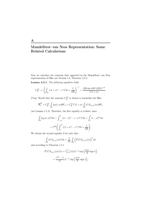
kH (t, u)dWu = CH Γ (1 + α)
(2)
R
α (I− 1(0,t) )(x)dWx
(see Lemma 1.1.3). Therefore, the first equality is evident, since
0 R t
(kH (t, u))2 x)α )2 dx +
k n
2H
2
.
C . n2
(B.0.12)
References
[AOPU00] Aase, K., Øksendal, B., Privault, N., Ubøe, J.: White noise generalization of the Clark-Haussmann-Ocone theorem with applications to mathematical finance. Finance Stoch., 4, 465–496 (2000) [AS96] Abry, P., Sellan, F.: The wavelet-based synthesis for fractional Brownian motion proposed by F. Sellan and Y. Meyer: Remarks and fast implementation. Appl. Comp. Harmon. Analysis, 3, 377–383 (1996) [AS95] Adler, R.J.; Samorodnitsky, G.: Super fractional Brownian motion, fractional super Brownian motion and related self-similar (super) processes. Ann. Prob., 23, 743–766 (1995) [ALN01] Al` os, E., Le´ on, I.A., Nualart, D.: Stratonovich stochastic calculus with respect to fractional Brownian motion with Hurst parameter less than 1/2. Taiwanesse J. Math., 5, 609–632 (2001) [AMN00] Al` os, E., Mazet, O., Nualart, D.: Stochastic calculus with respect to fractional Brownian motion with Hurst parameter less than 1/2. Stoch. Proc. Appl., 86, 121–139 (2000) [AMN01] Al` os, E., Mazet, O., Nualart, D.: Stochastic calculus with respect to Gaussian processes. Ann. Prob., 29, 766–801 (2001) [AN02] Al` os, E., Nualart, D.: Stochastic integration with respect to the fractional Brownian motion. Stoch. Stoch. Rep., 75, 129–152 (2002) [And05] Androshchuk, T.: The approximation of stochastic integral w.r.t. fBm by the integrals w.r.t. absolutely continuous processes. Prob. Theory Math. Stat., 73, 11–20 (2005) [AM06] Androshchuk, T., Mishura Y.: Mixed Brownian–fractional Brownian model: absence of arbitrage and related topics. Stochastics: Intern. J. Prob. Stoch. Proc., 78, 281–300 (2006) [AG03] Anh, V., Grecksch, W.: A fractional stochastic evolution equation driven by fractional Brownian motion. Monte Carlo Methods Appl. 9, 189–199 (2003)
牛顿-拉夫逊潮流计算中检测雅可比矩阵奇异性和网络孤岛的新方法
由 ( 式可得:I 【 0由于 D是对角矩 3 ) = 阵, , 因此 至少有一对角元 素为 0 。 因为 U= UL D D ,VL 设该潮流计算 是 n 节点 系统 。 所以( ) 2) 2 或( 工 a b弋有一个成立 , U 中有一 H子矩阵奇异 ,那 么 H矩阵各 个列向量线 性相 即 n 一1 零行 或 中有一零列 。 u 中行为零 , 是行相关 隋况 ;丰中列 为 关 , : 这 L 即 - = ( 不全为 0 q 0 ) 零, 这是列相关 隋况。 其 中: 是 H矩 阵的列 向量 ,1是相关 系 c T A矩 阵奇异 , 那么 A矩 阵行 向量 、 向量线 列 数 。由潮流雅可 比矩阵元素计算可知 : 性相关 , 即: 对 同一节点 , 素和 J 素的计 算具 有完 H元 元 全相似 的表达式 ,因此 ,矩 阵的各个列 向量也 J (a 4) 应满足( , 即:
中国新技术新产 品
一7
!
C ia N w T c n l ge n r d cs h n e e h oo isa d P o u t
高 新 技 术
新型停 水 自动关 闭阀结构 、 点及操作要 点 特
张金龙 曹 艳
( 西安航 空技 术高等专科学校机械 工程 系, 陕西 西安 7 0 7 ) 10 7
中图分 类 号 : 4 . 文献标 识 码 : G6 45 A
。
I 言 。在 日常生 活 中 , 前 由于停 水时 忘记 关 闭 阀门 , 水 时 也没 能及 时 关 闭 阀门 , 来 造成 水 资源 浪 费甚 至形 成安 全 隐 患 的情况 屡 见不 鲜 。 着全 民节 水 概念 不 断深入 人 心 , 一 问 随 这 题 引起 各方 关 注 。 因此 急 需设 计 一 款可 以在 停 水 时 自动关 闭 的水 阀 ,它 能够 在停 水 后 即 使 人们 忘记 关 闭 水 龙 头 也 能实 现 自动 关 闭 , 而再 次 来水 时 不 至于 出 现水 患 的情 况 ,能够 有 效 的节 约水 资源 。 要 实 现 自动 关 闭 功 能首 先 要 有 动 力 , 这 方 面可 以借 助 磁性 元件 的磁 力 、弹性 元 件 的 弹力 、 力 等外 力 , 时考 虑供 水 和停 水 时 的 重 同 水 压变 化 , 通过 联 动机 构实 现 。 2停 水 自动关 闭 阀 的结 构 及 特点 。利用 水 压 、 力 等 力 学 特 性 , 过 一 系 列 的实 验 、 重 经 改 进 , 发 出一 种 简单 、 行 的带 有 停水 自锁 研 可 机 构 的水 阀 。 款 水 阀为纯 机 械构 造 , 阀体 这 以 为 主体 框 架 , 有 阀 芯 、 封 圈 、 心 轮 以及 配 密 偏 手柄 , 无弹 性元 件 , 作状 况 不 受环 境 和时 间 工 的 限制 , 构 简 单 , 价 低 廉 并 方 便拆 换 , 结 造 整 体 可靠 性 高 。 停 水 自动关 闭 阀结 构 原 理 如 图 1 示 , 所 实 物 如 图 2所示 。序号 l 水 阀 的偏 心轮 , 为 2 为 0 型密 封 圈 , 为 V型 密封 圈 , 阀体 , 3 4为 5 为 阀芯 , 销 轴 , 手 柄 。 阀体 4是 主 框 6为 7为 架 , 来装 配其 它 元 件 , 进 水 口和 出 水 口; 用 有 阀芯 5的顶 端 与末 端分 别 装有 V 型密 封 圈 3 和 0 型 密 封 圈 2v 型 密 封 圈 3利 用 其 锥 面 , 与 阀体 4内部 锥 面 配合 实 现 停 水 时 密 封 , 而 0型密 封 圈 2与 阀体 4内壁 的接 触 实 现来 水 时对 水 阀末 端 的密 封 ,在 阀 芯 5的 中部 开两
薛定谔—麦克斯韦尔方程径向解的存在性和多重性(英文)
In 1887, the German physicist Erwin Schrödinger proposed a radial solution to the Maxwell-Schrödinger equation. This equation describes the behavior of an electron in an atom and is used to calculate its energy levels. The radial solution was found to be valid for all values of angular momentum quantum number l, which means that it can describe any type of atomic orbital.The existence and multiplicity of this radial solution has been studied extensively since then. It has been shown that there are infinitely many solutions for each value of l, with each one corresponding to a different energy level. Furthermore, these solutions can be divided into two categories: bound states and scattering states. Bound states have negative energies and correspond to electrons that are trapped within the atom; scattering states have positive energies and correspond to electrons that escape from the atom after being excited by external radiation or collisions with other particles.The existence and multiplicity of these solutions is important because they provide insight into how atoms interact with their environment through electromagnetic radiation or collisions with other particles. They also help us understand why certain elements form molecules when combined together, as well as why some elements remain stable while others decay over time due to radioactive processes such as alpha decay or beta decay.。
(2008)Dimensionality reduction: A comparative review
L.J.P. van der Maaten ∗ , E.O. Postma, H.J. van den Herik
MICC, Maastricht University, P.O. Box 616, 6200 MD Maastricht, The Netherlands.
22 February 2008
the number of techniques and tasks that are addressed). Motivated by the lack of a systematic comparison of dimensionality reduction techniques, this paper presents a comparative study of the most important linear dimensionality reduction technique (PCA), and twelve frontranked nonlinear dimensionality reduction techniques. The aims of the paper are (1) to investigate to what extent novel nonlinear dimensionality reduction techniques outperform the traditional PCA on real-world datasets and (2) to identify the inherent weaknesses of the twelve nonlinear dimenisonality reduction techniques. The investigation is performed by both a theoretical and an empirical evaluation of the dimensionality reduction techniques. The identification is performed by a careful analysis of the empirical results on specifically designed artificial datasets and on the real-world datasets. Next to PCA, the paper investigates the following twelve nonlinear techniques: (1) multidimensional scaling, (2) Isomap, (3) Maximum Variance Unfolding, (4) Kernel PCA, (5) diffusion maps, (6) multilayer autoencoders, (7) Locally Linear Embedding, (8) Laplacian Eigenmaps, (9) Hessian LLE, (10) Local Tangent Space Analysis, (11) Locally Linear Coordination, and (12) manifold charting. Although our comparative review includes the most important nonlinear techniques for dimensionality reduction, it is not exhaustive. In the appendix, we list other important (nonlinear) dimensionality reduction techniques that are not included in our comparative review. There, we briefly explain why these techniques are not included. The outline of the remainder of this paper is as follows. In Section 2, we give a formal definition of dimensionality reduction. Section 3 briefly discusses the most important linear technique for dimensionality reduction (PCA). Subsequently, Section 4 describes and discusses the selected twelve nonlinear techniques for dimensionality reduction. Section 5 lists all techniques by theoretical characteristics. Then, in Section 6, we present an empirical comparison of twelve techniques for dimensionality reduction on five artificial datasets and five natural datasets. Section 7 discusses the results of the experiments; moreover, it identifies weaknesses and points of improvement of the selected nonlinear techniques. Section 8 provides our conclusions. Our main conclusion is that the focus of the research community should shift towards nonlocal techniques for dimensionality reduction with objective functions that can be optimized well in practice (such as PCA, Kernel PCA, and autoencoders).
固体物理词汇汉英对照

元素的电负性 Electronegativities of elements
元素的电离能 Ionization energies of the elements
元素的结合能 Cohesive energies of the elements
六方密堆积 Hexagonal close-packed
费密-狄喇克分布函数 Fermi-Dirac distribution function
费密电子气的简并性 Degeneracy of free electron Fermi gas
费密 Fermi
费密能 Fermi energy
费密能级 Fermi level
费密球 Fermi sphere
正交晶系 Orthorhombic crystal system
正则振动 Normal vibration
正则坐标 Normal coordinates
立方晶系 Cubic crystal system
立方密堆积 Cubic close-packed
四方晶系 Tetragonal crystal system
金刚石结构 Diamond structure
金属的结合能 Cohesive energy of metals
金属晶体 Metallic Crystal
转动轴 Rotation axes
转动-反演轴 Rotation-inversion axes
转动晶体法 Rotating crystal method
切应变 Shear strain
八画
周期性重复单元 Periodic repeated unit
底心正交格子 Base-centered orthorhombic lattice
混沌动力学模型

混沌动力学模型混沌动力学模型是一种描述非线性系统行为的数学模型。
它的核心概念是混沌现象,即系统的微小变化会引起巨大的效应,使系统表现出不可预测的行为。
混沌动力学模型的研究对于理解和揭示自然界中复杂系统的行为规律具有重要意义。
混沌动力学模型的起源可以追溯到20世纪60年代,由美国数学家Edward Lorenz提出。
他在研究大气环流系统时,发现微小的初始条件变化会导致天气预报的巨大误差。
这一发现引发了他对非线性系统的研究,最终形成了混沌动力学模型。
混沌动力学模型的核心方程是著名的洛伦兹方程,它描述了一个简化的大气对流系统。
洛伦兹方程是一个三维非线性常微分方程组,它的解决过程展现了混沌现象。
洛伦兹方程的形式如下:dx/dt = σ(y - x)dy/dt = x(ρ - z) - ydz/dt = xy - βz其中,x、y、z是系统的三个状态变量,t是时间,σ、ρ、β是系统的参数。
通过调节参数的值,可以观察到不同的系统行为,包括稳定状态、周期运动和混沌运动。
混沌动力学模型的研究揭示了非线性系统的一些重要特性。
首先是灵敏依赖于初值条件,微小的初始条件变化会导致系统演化出完全不同的轨迹。
这意味着我们无法准确预测系统的未来行为,只能给出可能的演化趋势。
其次是周期倍增现象,系统在某些参数值下会表现出周期倍增的行为,即周期长度不断加倍,最终进入混沌状态。
最后是拓扑混沌,非线性系统的相空间结构呈现出复杂的拓扑特征,例如奇异吸引子和分岔图等。
混沌动力学模型的研究不仅在天气预报、气候学等领域有重要应用,还在物理学、生物学、经济学等多个学科中发挥着重要作用。
通过混沌动力学模型,我们可以更好地理解和解释自然界中的复杂现象,为科学研究和实践提供指导。
混沌动力学模型的研究也给我们带来了一些启示。
首先是复杂系统的不可预测性,即使是简单的非线性系统也可能表现出混沌行为,我们无法准确预测系统的未来演化。
其次是系统的微小变化可能引起巨大效应,这对于控制和管理复杂系统具有挑战性。
floquet bloch定理

floquet bloch定理
Floquet定理和Bloch定理都是线性周期系统中的重要定理。
Bloch定理(也称为Bloch理论或Bloch波函数)描述了处于周期性晶格结构中运动的电子被周期性调幅的波函数形式,即波矢量k和振幅u(r)的乘积。
这个定理是由菲利克斯·布洛赫在1928年研究晶态固体的导电性时首次提出的,但其数学基础在历史上曾由乔治·威廉·希尔(George William Hill,1877年),加斯东·弗洛凯(Gaston Floquet,1883年)和亚历山大·李雅普诺夫(Alexander Lyapunov,1892年)等独立地提出。
Floquet定理则表述了一个具有周期系数的线性常微分方程可以通过约化成为一个常系数的常微分方程。
考虑方程:x ˙ = A(t)x\dot{x}=A(t)xx˙=A(t)x其中A(t)关于t是T周期的。
通过一些操作,可以将这个周期系数的线性方程约化为常系数方程。
这个定理具有非常重要的意义,因为它的高度概括性,使得它能应用在自然科学的很多领域,量子力学当中有这样一个结论:电子在一类周期势中运动时,其定态波函数总可以表示成一个平面波乘以适当的与势同周期的周期函数。
在Floquet定理中正是Φ(t)=P(t)e−BTP\Phi(t)=P(t)e^{-BT}\Phi(t)=P(t)e−BT。
以上信息仅供参考,如有需要,建议查阅数学、物理相关书籍或咨询数学、物理专家。
- 1、下载文档前请自行甄别文档内容的完整性,平台不提供额外的编辑、内容补充、找答案等附加服务。
- 2、"仅部分预览"的文档,不可在线预览部分如存在完整性等问题,可反馈申请退款(可完整预览的文档不适用该条件!)。
- 3、如文档侵犯您的权益,请联系客服反馈,我们会尽快为您处理(人工客服工作时间:9:00-18:30)。
a r X i v :0806.2516v 1 [q u a n t -p h ] 16 J u n 2008Dynamics of Bloch vectors and the channel capacity of a non identicalcharged qubit pairN.Metwally,M.Abdel-Aty and A.-S.F.Obada ∗Mathematics Department,College of Science,Bahrain University,32038Bahrain∗Mathematics Department,Faculty of Science,Al-Azhar University,Cairo,Egypt We have considered a system of two superconducting charge qubits capacitivelycoupled to a microwave resonator.The dynamics of the Bloch vectors are inves-tigated for different regimes.By means of the Bloch vectors and cross dyadic we quantify the degree of entanglement contained in the generated entangled state.We consider different values of the system parameters to discuss the dynamics of the channel capacity between the qubits.We show that there is an important role played by initial state settings,coupling constant and the mean photon number on generating entangled state with high degree of entanglement and high capacity Keywords:Charged Qubit,Bloch vectors Entanglement,Capacity .1IntroductionQuantum entanglement is a quantum mechanical phenomenon in which the quantum states of two or more objects have to be described with reference to each other,even though the individual objects may be spatially separated.It is an essential component in many quantum information processing applications,such as quantum computation [1],teleportation [3]and cryptography [2]and dense coding [4,5].Therefore,it is essential to create and manipulate entangled states for quantum information tasks.The basic element of the quantum information is the quantum bit (qubit)which is considered as a two level system.Consequently,most of the research concentrate to generate entanglement between two level systems.Among these systems,superconducting charged qubits i.e.the Cooper pair box [6,12].In the last years the generated entangled states between Cooper pairs has been received a lot of attenuation.This is due to its properties as a two-level quantum system,which makes it a candidate as a qubit in a quantum computer [7,8].Also,recently these types of charged particles has been used to implement a Shor’s factor-ization [9],Deutsch-Jozsa algorithm [10],the Grover search algorithm protocol [11],and the quantum computing with a single molecular ensemble.On the other hand theses charged pairs have been used to realize a controlled phase gate [13].All theseapplications have encouraged different authors to study the entangled properties of these systems.As an example,the entanglement between two superconducting qubits has been generated by the interaction with nonclassical radiation[14].Ro-drigues et al.have evaluated the entanglement of superconducting charge qubits by homodyne measurement[15,16].The entropy squeezing and the emission spectra of a single-cooper pair have been investigated[17].On the other hand,it is known that the Bloch vector gives one of the possible descriptions of N-level quantum states,because it is defined as a vector whose com-ponents are expectation values of some observables.So,we can use it to describe the density operator of any system[18].These vectors(called coherent vectors),play a central role in quantifying the degree of entanglement,where Englert[19]has used it to evaluate the entanglement dyadic which represent a measure of the degree of entanglement.Addressing this issue with Cooper pair box systems is the main aim of the present paper.In this article we propose to study a system of two-Cooper pairs interacting with a single cavity mode.We investigate the dynamics of the polarized vector for each individual qubit and the channel capacity of the entangled Cooper pair for different values of the system parameters.This paper is organized as follows.In section2, we introduce our model and its solution.We devote section3,to investigate the relation between the Bloch vectors and the quantum entanglement.In section4, we investigate the effect of the structure of the initial state and the mean photon number on the transmission rate of information between two parties via the channel capacity.Finally,we end up with our conclusion.2Model and its solutionOur system consists of two superconducting charge qubits each coupled capacitively to a strapline resonator.Each charged qubit consists of a small superconducting is-land with a Cooper pair charge Q.This island connected by two identical Josephson junctions,with capacity C j and Josephson coupling energy E j,to a superconducting electrode.This system can be describe as a pair of two-level systems coupled to a simple harmonic oscillator.The charging energy of the qubits and their coupling to the resonator can be controlled by the application of magnetic and electricfields. By using the a rotating wave approximation,the system can be described by theHamiltonian[15].1H= ω(a†a+√2|α|2).Now we can write the time evolution of the density operator in the formρ(t)=U(t)ρ(0)U†(t),(2) where U(t)=exp(−iHt/ℏ)is the time-dependent unitary operator andρ(0)= |ψ(0) ψ(0)|.Since the invariant sub-space of the global system can be considered as a set of complete basis of the atom-field.Since,we are interested in the contribution of the Bloch vector in quantifying the degree of entanglement,we express the density operatorρc(t)of the system charged system by means of the Bloch vector for each qubit and the cross dyadic.After tracing out the state of thefield one gets the state of the charged qubit as,1ρc(t)=while for the second qubit,t x (t )=A n +1(t )B ∗n (t )+B n (t )A ∗n +1(t )+C n +1(t )D ∗n (t )+D n (t )C ∗n +1(t ),t y (t )=i −A n +1(t )B ∗n (t )+B n (t )A ∗n +1(t )−C n +1(t )D ∗n (t )+D n (t )C ∗n +1(t ) ,t z (t )=|A n (t )|2−|B n (t )|2+|C n (t )|2−|D n (t )|2,(5)In addition to the elements of the cross dyadic,↓−→@rrowCc xx =A n +2(t )D ∗n (t )+B n (t )C ∗n (t )+C n (t )B ∗n (t )+D n (t )A ∗n +2(t ),c xy =i −A n +2(t )D ∗n (t )+B n (t )C ∗n (t )−C n (t )B ∗n (t )+D n (t )A ∗n +2(t ) ,c xz =A n +1(t )C ∗n (t )−B n +1(t )D ∗n (t )+C n (t )A ∗n +1(t )−D n (t )B ∗n +1(t )c yx =i −A n +2(t )D ∗n (t )−B n (t )C ∗n (t )+C n (t )B ∗n (t )+D n (t )A ∗n +2(t ) ,c yy =−A n +2(t )D ∗n (t )+B n (t )C ∗n (t )+C n (t )B ∗n (t )−D n (t )A ∗n +2(t ),c yz =i −A n +1(t )C ∗n (t )+B n +1(t )D ∗n (t )+C n (t )A ∗n +1(t )−D n (t )B ∗n +1(t ) ,c zx =A n +1(t )B ∗n (t )+B n (t )A ∗n +1(t )−C n +1(t )D ∗n (t )−D n (t )C ∗n +1(t ),c zy =i −A n +1(t )B ∗n (t )+B n (t )A ∗n +1(t )−C n +1(t )D ∗n (t )+D n (t )C ∗n +1(t )c zz =|A n (t )|2−|B n (t )|2−|C n (t )|2+|D n (t )|2,(6)where,A n (t )=∞ n−a µn )−cos(t √µn )+νn cos(t√µn −νn cos(t√νn ),B n (t )=∞ n−iaRγn√µn )+(1−R 2)β2n −νnνnsin(t √µn −νn((1−R 2)γ2n−µn )sin(t √νn ),C n (t )=∞ n =0iaγn √µn )−(1−R 2)β2n −νnνnsin(t √µn −νn (1−R 2)γ2n+µn µn sin(t√√νn ) ,D n (t )=∞ n =0−bµn )−cos(t √µn )+νn cos(t√µn −νncos(t √νn ) ,(7)and,γn=√n+2µn=1δ2n−4∆2n),νn=1δ2n−4∆2n)δn=(1+R2)(γ2n+β2n),∆n=(1−R2)2β2nγ2n and R=λ22)and b=e iφsin(θ102030405060Scaled time0.20.40.60.81(a)102030405060Scaled time0.20.40.60.81(b)Figure 1:The Bloch vectors as functions of the scaled time.The two-qubit system is prepared initially in an excited state |e 1,e 2 ,and the field starts from a coherent state with a mean-photon number ¯n =20.The solid curves for the first qubit whilethe dot curves for the second qubit.The relative coupling is (a)for R =0.003(b)R =0.9.Bell states has zero Bloch vectors.So,as the Bloch vectors decrease,the possibility for obtaining an entangled state with high degree of entanglement increases.So,by using a suitable values of the coupling constant,one can control the Bloch vectors and consequently it is possible to generate an entangled state with high degree of entanglement.In Fig.(2),we plot the Bloch sphere,with radius equal 0.4units,at specific time in the interval [10.2−11.6],where we consider that the charged qubits are prepared in the excited state and R =0.9.The amplitude and the direction of the Bloch vector for the first qubit are shown.One can see that at t =10.2,the Bloch vector parallel to y -axis and it has a large value.As the time increases (say t =10.3,10.4),the Bloch vector inside the sphere and it could great or equal 0.4.As the time increases further,the Bloch vector appears in a different direction and its amplitude shrinks,this is shown for t =10.5.As time increases more the length of the Bloch vector increases and its direction change.In Fig.(3),we assume that the charged system is prepared in the partiallyentangled state a ee +b gg .For small values for the relative coupling the generalbehavior of the two vectors is somehow similar with small diffparing Figs.(1a )and (2a ),we see that the minimum point of the Bloch vector is decreasedfor the partial entangled state,which means that,using this class of the initial state,it will be more efficient to generate entangled state with high degree of entanglement.For large values of the relative coupling constant,R =0.9,the behavior of the two.7.6Figure2:The Bloch sphere for a charged system prepared initially in an excited state with¯n=20,R=0.9.The thick line represents the length of the Bloch vector for thefirst qubits.Bloch vectors are similar.For a specific time one of the Bloch vectors reaches to zero,in this case there is a maximum entangled state generated between the two charged qubit,In Fig.(3c),we consider the mean photon number¯n=10and R is small.In this case,we can see that the minimum point of the Bloch vectors is very small compared with that depicted in Fig.(3a).Also,the Bloch vector for the second qubit is shrunk more for small values of the mean photon number.This phenomena is clearly appeared in Fig.(3d),where we consider a large value of the coupling constant.In additional to the coincidence of the behavior of the Bloch vector for the two qubits,the two vectors are shrinking more.So,in this case the possibility of generating entangled state with high degree of entanglement is increased.4Degree of EntanglementTo quantify the degree of entanglement between the two charged qubits,we use a measure which is defined by means of the Bloch vectors and the cross dyadic.Wedefine the entangled dyadic as↓−→@rrowE =↓−→@rrowC −s ↓→t(8)where ↓−→@rrowc is a 3×3matrix which is defined by(6)and s ↓→t is also 3×3matrix whose elements can be obtained from (4)and (5).The degree of entanglement is defined byDoE =tr {↓−→@rrowE T·↓−→@rrowE }(9)where ↓−→@rrowE Tis the transpose matrix of the dyadic ↓−→@rrowEThe amount of entanglement between the entangled charged qubits is shown in Fig.4,in which we consider different regimes.In the first regime,we assumethat the two qubits are prepared initially in the following excited state ψ(0) c=eewhile the field starts from a coherent state with a mean photon number ¯n =20.InFig.(4a ),we see that for a small value of the coupling constant (say R =0.003),there is no any quantum correlation between the two charged qubit expect on the interval [19.2-40.5],where in this interval the Bloch of the second qubit decreases.102030405060Scaled time0.20.40.60.81(a)102030405060Scaled time0.20.40.60.81(b)102030405060Scaled time0.20.40.60.81(c)102030405060Scaled time0.20.40.60.81(d)Figure 3:The same as Fig.(1)but the charged qubits are prepared initially a partial entangled state.102030405060Scaled time0.20.40.60.8(a)102030405060Scaled time0.20.40.60.81(b)Figure 4:The degree of entanglement for a charged system prepared initially in an excited state with ¯n =20.(a)For R =0.003(a)excited (b)R =0.9.This means that in this intervals,the three subsystems (the two charged qubits and the field)interact with each others.Also,from this figure,we can see that the maximum amount of entanglement is obtained at the minimum point of the Bloch vectors of both qubits.This phenomena,also,is shown in Fig.(4b ),where we consider R =0.9.As soon as the interaction starts,(scaled time is greater than zero),the entangled state starts to be generated.It is obvious to realize that the development of the entanglement depends on the dynamics of the Bloch vectors.The effect of different setting of the initial state of the charged qubit is seen in Fig.(5),where we assume that the system is prepared initially in a partially entangled state.Fig.(5a ),is devoted to consider a weak correlation case (say R =0.003).102030405060Scaled time0.20.40.60.81(a)102030405060Scaled time0.20.40.60.81(b)Figure 5:The degree of entanglement for a charged system prepared initially in partially entangled states with ¯n =20.(a)For R =0.003(a)excited (b)R =0.9.From thisfigure it is clear that the degree of entanglement decreases with time until it reaches a minimum point atλ1t≃15.From Fig.(3a),we see that the Bloch vector for both qubit are maximum and consequently the degree of entanglement will be minimum according to the definition(9).In the interval[40−60],the degree of entanglement starts to increase another time,where in this interval of time the Bloch vector decrease(see Fig.(3a)).For a strong correlation the dynamics is seen in Fig.(5b).It is clear that the degree of entanglement is much stronger,where the efficiency of generating entangled state in this case is much higher.Also,the evolvement of the degree of entanglement depends on the evolvement of the Bloch vector for each qubit.In this context it is very important to investigate the evolvement of the degree of entanglement for different values of the mean photon number¯n.We choose the case for the weak coupling,where R=0.003.In Fig.(6a),we assume that the system has been processed in advance in an excites state.The usual effect of the mean photon number is seen where the Rabi oscillation is shifted to the left.In this case the maximum amount of entanglement is smaller than that depicted for ¯n=20(Fig.(4a)).But on the other hand,there is an entangled state is generated in the interval[50−60],while on the corresponding interval the charged system behaves as a product state.In Fig.(6b),we plot the degree of entanglement for a charged qubit is prepared in partially entangled state.In this case the degree of entanglement is much better than that shown in Fig.(5a),where¯n=20.So,For the weak interaction one can generate an entangled state between the two charged qubits by reducing the number of photons in the cavity mode.5The channel CapacityIn this section we investigate the effect of the structure of the initial state and the mean photon number on the transmission rate of information from a sender(Alice), to a receiver(Bob).This task can be performed by employing the dense coding protocol[3],[20,21].The main idea of this protocol is that,Alice and Bob share an entangled qubit pair.They used it as a channel,where Alice can encode two classical bits in her qubit by using local operation.Alice sends her qubit to Bob, who will try to decode the information.The amount of information gained by Bob depends on the capacity of the channel.In this context,we try to show how the capacity of the channel and hence the rate of transmit information depend on the102030405060Scaled time 0.10.20.30.4(a)102030405060Scaled time 0.20.40.60.8(b)Figure 6:The degree of entanglement for a charged system prepared initially in partially entangled states with ¯n =10,R =0.003.For (a)excited (b)partially entangled state.structure of the initial states,the relative coupling and the mean photon number.For N ×M state system,the dense coding capacity is given byC =logD A +S (ρB )−S (ρAB ),(10)where D A =N ,ρB =tr A {ρAB }and S (.)is the Von Numann entropy.Since we consider entangled two qubits,then our system is in 2×2dimension.Fig.5,shows the behavior of the capacity of the entangled quantum channel,where we consider the two charged qubits are in excited state.We investigate the effect of the coupling constant,the mean photon number and the setting of the initial state of the charged system.Fig.(7a ),shows the behavior of the channel capacity for a charged system with a strong coupling with the field,where we assume that R =0.9and the mean photon number ¯n =10.From this figure it is clear that the channel capacity for a charged system is prepared initially in a partially entangled state is much better than that if we start with a charged qubit in an excited state (product state).The effect of the mean photon number is seen if we take a look at Fig.(7b),where we consider ¯n =10.From this figure,we can see that the Rabi oscillations shrunk and shifted to the right as time increases.Due to the shrunk of the oscillations,we can see that the channel capacity increases a little bit as ¯n increases.From Fig.(4b )and Fig.(7b ),we can see that there is a strong relation between the degree of entanglement and the channel capacity and hence the rate of transform data.This maximum value of the channel capacity is obtained at a large degree of entanglement,as an example in the interval [0.2,0.8].Also,from equation (10),the capacity of the channel does notonly depend on the channel ρab ,but also on the individual state for the single qubit ρb .It is clear on the interval [10-20]as an example,the degree of entanglement is almost zero,but the capacity does not vanish.6ConclusionIn this paper we have studied in a non-standard way the dynamics of the Bloch vectors for two charged qubits.We investigate the dynamical behavior of the Bloch vector for each qubit.The shrunk,extension and the direction of these vectors are examined for different parameters of the charged system and the cavity field.We show for strong coupling between the filed and the charged system,the Bloch vector for the two qubits have the same behavior.But if one qubit has a weak coupling with the field (as the second qubit in our case),the behavior of the two Bloch vectors is different.Using the density matrix technique,we predict the existence of entangled states,where we consider an entanglement measure which depends on the two Bloch vectors and the cross dyadic and is called entangled dyadic.The relation between the evolvement of the Bloch vector and the degree of entanglement is shown,where for large values of the Bloch vectors,the degree of entanglement is minimum.It is shown that,for a charged qubit prepared initially in an entangled state,the amount of entanglement is much larger than that for any other choices.The role played00.20.40.60.811.20102030405060(a)Scaled Time 00.20.40.60.811.20102030405060(b)Scaled TimeFigure 7:The capacity of the channel where R =0.9The solid and dot curves for a charged system is prepared initially in a partially entangled and excited states respectively.(a)for ¯n =10,and (b)For ¯n =20.by the coupling constant and the mean photon number is cleared for generating entangled states and improving its degree of entanglement.Decreasing the mean photon number of the cavity mode is important to generate entangled state even the coupling between the qubits andfield is weak.The behavior of the channel capacity between the two charged qubits is ex-amined,using different regimes of preparing the initial state of the system.It is shown that the possibility of generating entangled state with high capacity and consequently high rate of transmission of information is much better if we start with a partially entangled state for the system.Also,the mean photon number plays a central role in the efficient of the channel capacity,where for small values of the mean photon numbers,the channel capacity is increased and consequently the transmission rate of information.References[1]D.P.DiVincenzo,Science,270255,(1995);A.K.Ekert and R.Jozsa,Rev.Mod.Phys.68733(1996).[2]A.K.Ekert,Phys.Rev.Lett.67661,(1991).[3]C.H.Bennett,G.Brassard,C.Crepeau,R.Jozsa,A.Peres and W.K.Woot-ters,Phys.Rev.Lett701895(1993).[4]C.H.Bennett and S.J.Wiesner Phys.Rev.Lett.692881(1993).[5]X.San Ma and A.Min Wang,mun.270465(2007).[6]M.Zhang,J.Zpu and B.Shao,Int.J.Mod.Phys.B164767(2002),W.Krechand T.Wanger,Phys.Lett A275159(2000),H.S.Ding,S.P.Zhao,G.H.Chen and Q.S.Yang,Physica C382431(2002).[7]Yu.Makhlin,G.Sch¨o n and A.Shnirman,Nature398305(1999);G.Sch¨o n,Yu.Makhlin and A.Shnirman,Physica C352113(2001);J.Q.You and F.Nori,Physica E1833(2003).[8]G.Wendin,R.Soc.Lond.A3611323(2003),A.Niskanen,J.Vartiainen,andM.Salomaa,Phys.Rev.Lett.90197901(2003).[9]J.Vartiainen, A.O.Niska,M.Nakahara and M.Salomaa.Phys.Rev.A70012319(2004).[10]R.Fazio,J.Siewert,J.Mod.Opt.491245(200),N.Schuch,J.Siewert,physicastatus solidi233482(2002).[11]X.-Hu Zheng,D.Pin,Yu.Zheng Xue,and CAO Zhuo-Liang;Physica C.45376(2007).[12]K.Tordrup and K.Molmer Phys.Rev.A77,020301(R)(2008).[13]S.G.Schirmer,D.K.L.Oi,and A.D.Greentree,Phys.Rev.A71012325(2005).[14]J.Q.You,F.Nori,Physica E1833(2003).M.Paternostro1,G.Falci,M.Kim,and G.Palma,Phys.Rev.B69,214502(2004).[15]D.A.Rodrigues,C.E.A.Jarvis,B.L.Gyurffy,T.P.Spiller,J.F.Annett J.Phys.:Condens.Matter,20075211(2008).[16]D.A.Rodrigues,T.P.Spiller,J.F.Annett,B.L.Gyurffy,J.Phys.:Condens.Matter19436211(2007).[17]M.Abdel-Aty,Laser Phys.,161356(2006);M.Abdel Aty,H.Abdel-Hameedand N.Metwally,Phycica C45229(2007).[18]L.Jak´obczyk,M.Siennicki,Phys.Lett.A286(2001)383;G.Kimura,Phys.Lett.A314,339(2003).[19]B.-G.Englert,P.Lougovski and E.Solano,Laser Phys.13355(2003).[20]S.Bose,V.Vedral and P.L.Knight,Phys.Rev.A57,822(1998);G.Bowen,Phys.Rev.A63,022303(2001);X.S.Liu,G.L.Long,D.M.Tong,F.Li,Phys.Rev.A65,022304(2002).[21]Qiu-Bo Fan and S.Zhang,Phys.Lett A348160(2006);T.Vertesi,Phys.Lett.A357(167)(2006).。