Sediment Transport Modeling Review—Current and
外文翻译---7000公斤级柴油混合电动汽车排放特性模拟
第1章外文翻译1.1外文译文7000公斤级柴油混合电动汽车排放特性模拟摘要:电动马达和电池相混合的内燃机技术可结合起来,减少燃料消耗和废气排放。
本文介绍了混合动力电动汽车的概念(混合电动汽车)适用于柴油发动机的卡车或货车车辆。
从先进的汽车驾驶模拟器的仿真结果表明,所需要的功率可以适当与内燃机引擎及电动机共享。
仿真也可以用来证明该技术对在驾驶性能方面的改进有用;此外,是适用于混合动力汽车并具有良好的燃油经济性和低排放性能的技术。
关键词:中央商务驾驶巴士时间表(CBDBUS)高燃料经济性测试驱动周期(FWFET),串联式混合动力电动汽车,并行式混合动力电动汽车。
1.介绍石油燃料的消耗和环境污染的问题促使科学家开发混合动力电动汽车,如高级的汽车和燃料电池汽车。
在这些方面努力中的很多研究人员已将其注意力集中到混合领域,有一种可以把电动汽车和内燃机的好处结合起来的切实可行的汽车类型。
很多国家已经参与到改善环境问题和发展高效燃料经济性的混合动力研究中。
混合动力电动汽车有两个以上的来源电力,但是通常使用内燃机和电动机的组合。
为防止能源浪费造成的不必要的操作或停止了的引擎,混合动力汽车电机的输出连接到电动源用生成的电力为电池充电。
"混合"一词是指在需要时使用此生成的电力驱动电机。
而混合动力汽车通常是指由内部燃烧发动机与发电机组合成的,电动马达是由安装在该的车辆内部的高电压电池给与电力供应。
当车辆移动时电池被充电。
混合动力被列为串联或并联混合动力汽车基于电动马达在汽车上的使用。
混合系列作为一个发电机使用引擎,并将生成的电力存储在一个电池中。
混合动力车辆的控制的发动机和电动机根据车速电源驱动效率最大化。
混合动力汽车使用电动机启动引擎;但是,当车辆是在运动或加速,引擎提供了大部分的动力而电机作为补充的电源。
踩刹车时要减速导致动能转换为存储在电池里的电能。
此外,该车辆停止时引擎和马达也同时停止;因此,当车辆停止甚至在运行时,没有任何能源被浪费即使发动机还在旋转。
长江河口悬浮泥沙向浙闽沿岸输运近期变化的遥感分析
长江河口悬浮泥沙向浙闽沿岸输运近期变化的遥感分析陈瑞瑞;蒋雪中【期刊名称】《海洋科学》【年(卷),期】2017(041)003【摘要】The construction of a number of dams in the Changjiang River basin (and in particular, large dams in the mainstream) has led to a sharp reduction in the amount of suspended sediment transported from the basin to the sea. This study was instigated to determine the effect on adjacent waters from a change in sediment source, and the paper focuses on spatial and temporal variations in suspended sediments from the Yangtze Estuary to Zheji-ang-Fujian Provincial coastal sea obtained from remotely sensed data. A reliable model is established (according to in-situ measurements in different seasons during 2014) to extract suspended sediment concentration (SSC) from Terra- moderate resolution imaging spectroradiometer (MODIS) images, and the SSC transport mechanism is stud-ied based on results of these analyses. Results reveal that the transportation of suspended sediment from the Yangtze Estuary to the south coast has an obvious seasonal variation and is driven by the monsoon and coastal ocean cur-rents. In spring, suspended sediment is transported as a strip from the Yangtze Estuary to Zhejiang-Fujian Provincial coastal water, and in late spring the suspended sediment transport is interrupted by Wenling coastal waters. In summer, a largeamount of suspended sediment is left stranded in the Yangtze Estuary and the Hangzhou Bay:these interruptions are obvious. In autumn, a continuous coastal suspended sediment strip gradually forms between mid-October and late November. In recent years, under the influence of reducing suspended sediment from the river basin into the estuary, the continuous suspended sediment strip in winter has been broken off prior to spring and recovery has been delayed in autumn.%利用2000~2015年Terra-MODIS(terra-moderate resolution imaging spectroradiometer,中等分辨率成像光谱仪)数据和2014年洪枯季现场数据建立泥沙反演模型,分析入长江河口泥沙大幅减少后河口表层悬沙向浙闽沿岸输运的时空变化和扩散形态.结果表明:(1)利用MODIS数据的二次型模型能够揭示长江口及邻近海域悬沙分布及输运特征,入海输运的长江口悬浮泥沙是浙闽沿岸连续悬浮泥沙带存在的物源;(2)受季风和沿岸流动力驱动,长江口悬沙向浙闽沿岸输运具有明显的季节性:春季,悬浮泥沙从长江口向浙闽沿岸呈条带状输运,春夏之交,南下的悬沙至温岭近岸海域出现中断现象;夏季,长江口大量悬沙滞留在长江口杭州湾近岸,仅有少量悬沙向南输运,泥沙带中断;秋季,10月下旬—11月中旬逐渐形成连续的近岸泥沙带;历冬至春,循环复始;(3)受近年来长江流域进入河口的泥沙减少影响,浙闽沿岸秋冬季连续的输沙带在春季提前断开,在秋季有推迟恢复的现象.本研究对于探究浙闽沿岸泥沙减少新格局,分析近海生态环境新变化具有重要意义.【总页数】13页(P89-101)【作者】陈瑞瑞;蒋雪中【作者单位】华东师范大学河口海岸学国家重点实验室,上海 200062;华东师范大学河口海岸学国家重点实验室,上海 200062【正文语种】中文【中图分类】TP79【相关文献】1.闽浙沿岸泥质沉积的物源分析 [J], 肖尚斌;李安春;刘卫国;赵家成;徐方建2.长江河口北槽近期盐淡水混合与悬沙输运研究 [J], 高敏;李占海;张国安;王志罡;李远;李九发;谢火艳3.闽浙沿岸上升流及其季节变化的数值研究 [J], 经志友;齐义泉;华祖林4.近2 ka闽浙沿岸泥质沉积物物源分析 [J], 肖尚斌;李安春;蒋富清;尤征;陈莉5.浙闽沿岸潮余流的空间变化 [J], 林其良;黄大吉;宣基亮因版权原因,仅展示原文概要,查看原文内容请购买。
ProceedingsoftheIMechE,PartBJournalofEngineering
Proceedings of the IMechE, Part B:Journal of Engineering Manufacture 《英国机械工程师学会志,B辑:“工程制造杂志”》Issue 3 Mar. 2015序号目次信息1 篇名:Thermal and mechanical effects of high-speed impinging jet in orthogonal machining operations: Experimental, finite elements and analytical investigations高速冲击射流在正交加工中的热机械效应:实验,有限元分析作者:Andrea Bareggi and Garret E O’Donnell2 篇名:A statistical analysis applied for optimal cooling system selection and for a superior surface quality of machined magnesium alloy parts用于镁合金零件优化冷却系统选择的统计分析作者:Bogdan Chirita, Gheorghe Mustea, and Gheorghe Brabie3 篇名:An analytical investigation on the workpiece roundness generation and its perfection strategies in centreless grinding无心磨削的工件圆度的产生及其完善对策研究作者:Qi Cui, Hui Ding, and Kai Cheng4 篇名:A study of the micro-machining process on quartz crystals using an abrasive slurry jet基于磨料浆射流的石英晶体微加工工艺研究作者:Huan Qi, Jingming Fan, and Jun Wang5 篇名:On the use of cyclic shear, bending and uniaxial tension–compression tests to reproduce the cyclic response of sheet metals循环剪切,弯曲和单轴拉压试验,再现金属板材的循环响应作者:Abbas Ghaei, Daniel E Green, Sandrine Thuillier6 篇名:Dimensional variation stream modeling of investment casting process based on state space method基于状态空间法的熔模铸造工艺尺寸变化作者:Changhui Liu, Sun Jin, Xinmin Lai7 篇名:Suspended SiC particle deposition on plastic mold steel surfaces in powder-mixed electrical discharge machining粉末混合电火花加工中的塑料模具钢表面悬浮颗粒沉积作者:Bülent Ekmekci, Fevzi Ulusöz, Nihal Ekmekci8 篇名:Unified variation modeling of sheet metal assembly considering rigid and compliant variations考虑刚性和柔性变化的板料装配统一建模作者:Na Cai, Lihong Qiao, and Nabil Anwer9 篇名:An approach to minimizing surplus parts in selective assembly with genetic algorithm用遗传算法优化选择装配多余零件的方法作者:Cong Lu and Jun-Feng Fei10 篇名:Parameter analysis and identification of the multiple-advanced manufacturing mode diffusion model多先进制造模式扩散模型的参数分析与辨识作者:Chaogai Xue, Haiwang Cao, and Yu Sheng11 篇名:Functional cause analysis of complex manufacturing systems using structure复杂制造系统应用结构的功能原因分析作者:MK Loganathan, Minu Shikha Gandhi, and OP Gandhi12 篇名:A novel artificial ecological niche optimization algorithm for car sequencing problem considering energy consumption考虑能量消耗的汽车排序问题的一种新的人工生态位优化算法作者:Sanqiang Zhang, Daoyuan Yu, Xinyu Shao。
井工煤矿无轨胶轮车全局调度模型

井工煤矿无轨胶轮车全局调度模型陈湘源1, 潘涛2, 周彬3(1. 国能榆林能源有限责任公司,陕西 榆林 719000;2. 国能信息技术有限公司,北京 100011;3. 北京航空航天大学 车路一体智能交通全国重点实验室,北京 100191)摘要:井工煤矿无轨胶轮车数量多,运输易受搬家倒面、突发事件等影响,传统的人工调度方法效率低,且易造成车辆闲置、空载、里程浪费等问题,而现有的辅助运输车辆调度方法大多面向固定任务使用离散事件优化的方案,将全局模型拆解为局部模型,缺乏对井工煤矿整体情况的分析。
针对上述问题,提出了一种基于百度工业求解器的井工煤矿无轨胶轮车全局调度模型,介绍了该模型中信息收集模块、数据建模模块和工业求解器模块设计方案,以及无轨胶轮车全局调度流程。
该模型采用基于“分批求解、迭代优化”的无轨胶轮车全局调度算法,由百度工业求解器基于动作调整启发式算法对车辆调度问题进行优化求解,解决了传统调度模型求解时间长、易陷入局部最优解等问题。
实验结果表明,基于百度工业求解器的井工煤矿无轨胶轮车全局调度模型较人工调度方法大幅降低了使用车次,提高了车辆运转效率,调度优化的求解时间低于基于Gurobi 求解器的局部调度模型,更适用于井下辅助运输场景下大规模复杂调度任务。
关键词:井工煤矿;辅助运输;无轨胶轮车;车辆调度;全局调度优化;百度工业求解器中图分类号:TD54 文献标志码:AGlobal scheduling model for trackless rubber-tyred vehicle in underground coal minesCHEN Xiangyuan 1, PAN Tao 2, ZHOU Bin 3(1. CHN Energy Yulin Energy Co., Ltd., Yulin 719000, China ;2. CHN Energy Information Technology Co., Ltd., Beijing 100011, China ;3. State Key Lab of Intelligent Transportation System, Beihang University ,Beijing 100191, China)Abstract : There are a large number of trackless rubber-tyred vehicles in underground coal mines. The transportation is easily affected by moving surfaces, emergencies, and other factors. Traditional manual scheduling methods are inefficient and prone to problems such as idle, empty, and wasted vehicles. However,existing auxiliary transportation vehicle scheduling methods mostly focus on fixed tasks using discrete event optimization schemes. It breaks down the global model into local models, and lacks analysis of the overall situation of underground coal mines. In order to solve the above problems, a global scheduling model for trackless rubber-tyred vehicle in underground coal mines based on Baidu industrial solver is proposed. The design scheme of the information collection module, data modeling module, and industrial solver module in this model are introduced, as well as the global scheduling process for trackless rubber-tyred vehicles. This model adopts a global scheduling algorithm for trackless rubber-tyred vehicles based on "batch solving and iterative optimization". The vehicle scheduling problem is optimized and solved by Baidu industrial solver based on action收稿日期:2023-01-03;修回日期:2023-12-10;责任编辑:李明。
Sediment transport trends and cross-sectional stability of a lagoonal tidal inlet on the C
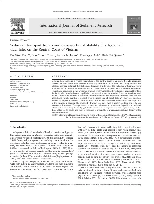
Original ResearchSediment transport trends and cross-sectional stability of a lagoonaltidal inlet on the Central Coast of VietnamDo Minh Duc a,n,Tran Thanh Tung b,Patrick McLaren c,Tran Ngoc Anh d,Dinh Thi Quynh aa Faculty of Geology,VNU University of Science,Vietnam National University,Hanoi334Nguyen Trai,Thanh Xuan,Hanoi,Viet Namb Faculty of Marine and Coastal Engineering,Thuyloi University,175Tay Son,Dong Da,Hanoi,Vietnamc SedTrend Analysis Limited,7236Peden Lane,Brentwood Bay,BC,Canada V8M1C5d Faculty of Meteorology,Hydrology and Oceanography,VNU University of Science,Vietnam National University,Hanoi,334Nguyen Trai,Thanh Xuan,Hanoi,Vietnama r t i c l e i n f oArticle history:Received28January2017Received in revised form26October2018Accepted2January2019Available online6January2019Keywords:LagoonTidal inletSediment Trend Analysis(STA)Tidal prismCross-sectional stabilitya b s t r a c tLagoonal tidal inlets are a typical morphology of the Central Coast of Vietnam.Recently,navigationchannels in these inlets have become increasingly threatened by siltation.This study analyses therelations between sediment distribution and transport trends(using the technique of Sediment TrendAnalysis-STA s)in the lagoonal system of the De Gi inlet and then proposes appropriate countermeasuresagainst sand deposition in the navigation channel.The STA identified three types of transport trends inthe De Gi inlet,namely dynamic equilibrium,net accretion,and net erosion.Processes associated withthe tidal prism have resulted in trends of sediment transport and deposition across theflood and ebbtidal shoals,which maintain a present cross-sectional area of about1000m2.However,longshoresediment transport from north to south resulting from northeast waves cause additional sand depositionin the channel.In addition,the effects of refraction associated with a nearby headland and jetty alsoincrease sedimentation.These processes provide the main reasons for sediment deposition in the De Giinlet.Short term and regular dredging helps to maintain the navigation channel.A system comprised ofthree jetties(north,south,and weir)is necessary to ensure the longterm cross-sectional stability of thenavigation channel.&2019International Research and Training Centre on Erosion and Sedimentation/the World Associationfor Sedimentation and Erosion Research.Published by Elsevier B.V.All rights reserved.1.IntroductionA lagoon is defined as a body of brackish,marine,or hypersa-line water impounded by a barrier,connected to the open ocean byone or more restricted inlets(Kaplin,1982;Kjerfve,1994;Phleger,1981).Geologically,a lagoon is an evolving coastal landform thatgoes from a shallow open embayment or estuary valley,to a par-tially enclosed back-barrier lagoon,and then,with progressiveinfilling,to a marsh or deltaic-filled lagoon(Nichols,1989).How-ever,a number of lagoons remain unfilled despite thousands ofyears of sedimentation due to a discontinuity in the geologicevolution(Adlam,2014).A review of definitions(Tagliapietra et al.,2009)provides a more detailed discussion.Coastal lagoons occupy about13%of the coastal areas world-wide with individual water surface area from less than1ha up to10,200km2(Duck&da Silva,2012).Barrier enclosed lagoons canbe further subdivided into four types,such as no barrier coastalbay,leaky lagoon with many wide tidal inlets,restricted lagoonwith several tidal inlets,and choked lagoon with narrow tidalinlets(Isla,1995;Kjerfve,1994).These sub-divisions are stronglyrelated to the dominant hydromorphological conditions observedin the lagoon(Duck&da Silva,2012).As a consequence of inten-sive urbanization in coastal zones,human activities can raiseimportant questions on lagoon ecosystem‘health’(e.g.,Bird,1994;Elliott,2011;Marotta et al.,2011)and the baseline or referenceconditions to which it is assessed(e.g.,da Silva&Duck,2001;Diniset al.,2006;Morris&Turner,2010).The internal balance betweenaccretion and erosion of lagoons may change leading to severalhazards such as sand deposition(e.g.,Duc et al.,2012;Duc et al.,2016;He et al.,2015),and coastal erosion(e.g.Blanco et al.,2015;Chalov et al.,2015;Duck&da Silva,2012;Meyer et al.,2016;Samaras&Koutitas,2014;Zhang et al.,2014).The cross-sectional area of lagoonal inlets that have been inexistence for a long time is in equilibrium under average hydraulicconditions.An empirical relation between cross-sectional area(A)and tidal prism(P)has been found(Jarrett,1976;LeConte,1905;O'Brien,1931;Stive et al.,2009).This relation is commonlyContents lists available at ScienceDirectjournal homepage:/locate/ijsrcInternational Journal of Sediment Researchhttps:///10.1016/j.ijsrc.2019.01.0011001-6279/&2019International Research and Training Centre on Erosion and Sedimentation/the World Association for Sedimentation and Erosion Research.Published by Elsevier B.V.All rights reserved.n Corresponding author.E-mail address:ducdm@.vn(D.M.Duc).International Journal of Sediment Research34(2019)322–334used to evaluate the cross-sectional stability of tidal inlets,pro-posed by Escoffier(1940)and later expanded by van de Kreeke (2004).The equilibrium of the inlet cross-sectional area is dynamic.It can be disturbed by extreme events,such as severe storms and riverfloods,and then returns to its equilibrium value (Escoffier,1940).It is of interest to understand the processes that are responsible for the observed cross-sectional stability.Determining these processes fromfield measurements requires extensive surveys which would result in costlyfield experiments and uncertain the outcomes(Tung,2011;Tung et al.,2012).The common alternatives to study these processes are the use of numerical models (e.g.,Davis,2013;Guan et al.,2015;Hoque et al.,2010;Kraus, 1998;Nichols&Boon,1994;Pacheco et al.,2008;van de Kreeke, 1985,2004).In this study,the alternative of using sediment transport trends is further considered.The purpose is to analyze the relations between sediment distribution and transport trends in a lagoon system where there is cross-sectional stability within the con-necting inlet.The method of cross-sectional stability helps to define a location and its cross section to be a stable channel from the hydrodynamic point of view.However,changes of bottom topography due to sediment transport and deposition cannot be taken into the account.Sediment Trend Analysis(STA)itself as a kinematic analysis(McLaren,2014)can help to define net trends of sediment transport which shows potential areas of deposition and erosion.Therefore,the STA and cross-sectional analysis support each other to define the spatial changes of cross-sectional stability. These results can then aid in defining appropriate counter-measures(e.g.,location,types,and geometrical characteristics of structures)against the navigational hazard resulting from sand deposition inside the entrance channel to the lagoon.2.Study areaThe De Gi estuary is connected to Nuoc Ngot lagoon which enters the East Sea in the Central part of Vietnam(Fig.1).The Nuoc Ngot lagoon encloses an area of about13km2.The Vinh Loi rocky headland with an area of1km2is composed of fractured granite and extends to a depth ofÀ3m.The lagoon shelters over1000 boats belonging to the Phu Cat and Phu My districts as well as a number of vessels from the Central area.Because of increasing sedimentation in the inlet a jetty,400m long,was built on its south side in2003.In spite of this,there has been little impact on the amount of deposition presently occurring.To meet the demand offishery development as well as to exploit the marine economic potential,the Phu Cat district has received an investment of Vietnamese Dong(VND)52billion from the Vietnamese government for constructing De Gi harbor. Beginning in1999,thefirst phase costing VND 4.5billion included a pier and revetment which have been inoperation Fig.1.Location of the study area.D.M.Duc et al./International Journal of Sediment Research34(2019)322–334323since2004.The construction proved its functionality and facilitated ship berthing.In the second phase,a breakwater was built on the southern bank of the inlet,the harbor entrance channel and basin was dredged(VND22.5billion),which were completed and have been in operation since September2006. Upon completion,De Gi harbor had designed yearly through-puts of12,000t of seafood and10,000t of other goods,as well as sheltering over1000vessels from storms.However,after the second phase of the project had been completed,the perfor-mance of the southern breakwater was poor and dredging the channels and basin largely was ineffective.Currently in the middle of the channel a wide shoal has formed,with elevation þ2m and occupies over2/3the channel width(Fig.2).At the shore-connected end of the breakwater,sand has been passing through the structure,causing sedimentation in the channel. From time to time,fishing vessels accessing the harbor have been sunk by waves,causing fatalities and loss of property.3.Methods3.1.Field survey and measurementsTopographical mapping on land was done using a Real Time Kinematic Digital Global Positioning System(RTK DGPS)(Magen-llan Z-Max equipment)with the data converted to the national datum.Water depth data,collected by echosounder in April2013 during calm wave conditions,was corrected to mean water level providing the bathymetry of both the lagoon and the sea.Wave characteristics were monitored with an Acoustic Wave and Current Profiler(AWAC)system,and included wave height, period,and direction.Thefirst period of the survey was done from September29to October5,2012,to characterize the northeast wave-dominated season that also corresponds to the region's rainy season.The second period was during the dry season and when waves dominate from the east and southeast.It was implemented from June3to11,2013.During both periods,water levels were monitored hourly at the An My Bridge and near the entrance of the De Gi inlet(Fig.3).3.2.Sediment trend analysisA total of134sediment grab samples were retrieved in the study area from the coastline to a depth of20m(Fig.3).Sampling sites were150to250m apart.The positions were determined with a GPS receiver with an accuracy of75m.Grain sizes were analyzed by sieving(sieve sizes:2,1,0.5,0.35,0.25,0.18,0.15, 0.125,0.1,0.074,and0.063mm,i.e.À1.0,0,1.0,1.51,2,2.47,2.74, 3.0,3.32,3.76,and4.0ϕ).The grain size parameters of mean, sorting,and skewness were calculated inϕunits(Folk,1966, 1980).A model to derive net sediment transport pathways wasfirst proposed by McLaren and Bowles(1985).According to the model, along the direction of net transport sediment can be either better sorted,finer,and more negatively skewed(measured inϕunits)or better sorted,coarser,and more positively skewed.The STA tech-nique is entirely empirical in that the observations are the grain-size distributions of the actual deposits.The derived patterns of transport provide an explanation for the observations by determining the“transport relations”among all the samples (i.e.changes in distributions are occurring that are non-random and their presence conforms to the STA theory as mathematically proven in McLaren and Bowles(1985)).In discovering the patterns of sediment movement,the results of the STA are,in themselves, self-validating.If a pattern could not be discovered,there are only two possible reasons:(i)the distance between samples was too large and could not account for all the sources that might be present;and(ii),which is a corollary of thefirst,not enough samples were taken to account for all the sources supplying sediment to the area under study.But if patterns are found,then it must be accepted that there are non-random changes occurring in the distributions and it is difficult to suggest a reason for such changes other than sediment transport.It can also be noted that STA theory is based on a single assumption–namely,a small or light particle is easier to move than a larger and heavier particle.Despite the large number of papers that have utilized STA theory in some way since its pub-lication,this assumption has never been challenged or discarded in favor of another assumption.Furthermore,there is nopossibleFig.2.Sand shoals in the De Gi inlet(a)two sand bars formed attached to the jetty,(b)moonsoon northeast wave attacks have washed out thefirst sand bar,but the more landward bar has expanded,(c)the sand shoal has enlarged and moved further toward the navigation channel,and(d)the area of the sand shoal has enlarged and a new sand bar has formed attached to the jetty.D.M.Duc et al./International Journal of Sediment Research34(2019)322–334324“bias ”associated with the mean,sorting,and skewness values that are derived from each of the collected samples.Once sediment pathways have been established,the computation and inter-pretation of what are termed “X-distributions ”along the pathways can describe the relative probability of each particle size being removed from deposit d 1and transported to deposit d 2(Hughes,2005).The X-distribution is de fined as a new distribution from the ratio of the grain-size distributions between two deposits.Based on the shape of the X-distribution along the sediment pathway relative to the shapes of the composite distributions d 1and d 2,McLaren and Bowles (1985)gave five scenarios for describing what is occurring along the pathway:(a)dynamic equilibrium,(b)net accretion,(c)net erosion,(d)total deposition I,and (e)total deposition II.The STA has been re-examined and applied in a large number of studies (e.g.,Avramidis et al.,2008;Chang et al.,2001;Duc et al.,2012,2016;Gao,1996;Gao &Collins,1991,1992;Héquette et al.,2008;Hughes,2005;Le Roux,1994;Le Roux et al.,2002;McLaren,2014;McLaren &Beveridge,2006;McLaren &Braid,2009;McLaren et al.,2007;McLaren &Singer,2008;McLaren &Teear,2014;Papatheodorou et al.,2012;Poizot et al.,2008;Rios et al.,2003).In this paper,STA was used as per the descriptions provided in Duc et al.(2016).3.3.The Escof fier diagramThe empirical cross-sectional area and tidal prism relation was presented as the Escof fier diagram (Escof fier,1940).It consists of a closure curve and an equilibrium velocity curve (Kraus,1998;Suprijo &Mano,2004;van de Kreeke,1998,2004).The equili-brium velocity curve represents the relation between equilibrium velocity and cross-sectional area.The closure curve represents therelation between the characteristic velocity,V c and the inlet cross-sectional area.A typical shape of the closure curve,V c (A)is shown in Fig.4.Starting at small values of A,V c increases,reaches a maximum,and with increasing values of A goes to zero.In most cases the closure curve is calculated by numerically solving the governing hydrodynamic equations for inlet velocity and water level for a given cross-sectional area,A.From this the tidal prism,P,is calculated.Channel Equilibrium Area (CEA)software,devel-oped by the Coastal Inlets Research Program,was used to de fine the equilibrium velocity curve and analyze cross-sectional stability of the De Gi inlet.4.Results4.1.Hydraulic characteristics4.1.1.Water levelWater levels observed at An My Bridge and the De Gi inlet's entrance are in phase and have similar fluctuation range.FortheFig.3.Topography,monitoring stations,and sediment sampling sites in the study area (De Giestuary).Fig.4.Escof fier diagram.D.M.Duc et al./International Journal of Sediment Research 34(2019)322–334325period of Sept.30–Oct.5,2012the maximum level was 0.56m at 23:00on Oct.4and the minimum -0.42m at 7:00on Oct.5local time (Fig.5).While in the period of 03–11June 2013,the max-imum level was 0.64m at 15:00on June 11,and the minimum level was -0.69m at 10:00on June 11local time (Fig.6).4.1.2.WavesThe wave characteristics measured with an AWAC system are listed in Table 1.The wave roses (Fig.7)show changes in wave characteristics in the two survey periods with north east wave-dominating in Sept.and Oct.2012and east wave-dominating in June 2013.The figure suggests highly variable hydrodynamic conditions for the northeast waves.The results show similar wave characteristics to longterm monitoring stations as presented in Trinh et al.(2011)and Tung (2011).4.2.Sediment distributionEight types of surface sediment were de fined based on grain-size characteristics and areas of distribution.Their characteristics and distribution are listed in Table 2and shown in Figs.8–10.(1)Coarse sand in the lagoon is contained in a small area,mainlyin front of the La Tinh river mouth located to the north of the area shown in Fig.8.Found to a depth of À1m the mean grain size is 0.6ϕ.The sorting coef ficient is 1.6ϕ(poorly sorted)and the skewness is positive.(2)Fine sand in the lagoon has a relatively small distribution area.Mean grain size ranges from 2.7to 3.8ϕ,with an average value of 3.3ϕ.Adjacent to rivers the sand is characterized by poor sorting (1.0ϕ);elsewhere sorting tends to be very poor (2.6ϕ).In both areas,skewness is positive.(3)Lagoon coarse silt is found in a narrow band surroundingthe fine sand facies.This sediment has mean diameters of 4.0–4.9ϕwith an average value of 4.5ϕ.Sorting coef ficientsFig.6.Observed water level in June 2013survey.Table 1Wave and current characteristics at the De Gi estuary.Parameter2012survey 2013survey Average wave height (m) 1.40.32Average wave period (s)9.386.15Dominant wave direction 61.7°(NE)111.2°(SE)Current velocity (m/s)0.130.112Current direction169.5°(SE)178.7°(SE)Fig.5.Observed water level in September 2012survey.Fig.7.Wave rose at the De Gi estuary a)September 2012and b)June 2013.Table 2Surface sediment characteristics.Characteristics of sedimentValues (ϕ)MeanSorting (So)Skewness (Sk)(1)Lagoon coarse sand 0.61.60.1(2)Lagoon fine sand 2.7–3.8 1.0–2.60.5–0.6(3.3)*(1.8)(0.5)(3)Lagoon coarse silt4.0–4.9 2.7–3.40.5–0.8(4.5)(3.1)(0.7)(4)Lagoon fine –very fine silt5.1–7.4 2.6–3.70.2–0.5(5.4)(3.2)(0.3)(5)Nearshore coarse –medium sand 0.1–1.90.5–1.0À0.6to 0.1(1.0)(0.71)(À0.2)(6)Nearshore fine –very fine sand 2.5–3.40.4–1.6À0.1to 0.3(2.8)(0.6)(-0.1)(7)Offshore medium sand 1.8–1.90.5–0.7À0.5to 0.1(1.8)(0.6)(À0.2)(8)Offshore fine sand2.0–2.70.2–0.5À0.1to 0.3(2.4)(0.4)(-0.1)2.7–3.8(3.3)*:min –max (average)values.D.M.Duc et al./International Journal of Sediment Research 34(2019)322–334326Fig.8.Sediment distribution in the studyarea.Fig.9.Mean diameter of sediment.D.M.Duc et al./International Journal of Sediment Research 34(2019)322–334327vary from poorly sorted (2.7ϕ)to very poorly sorted (3.4ϕ)and skewness is positive.(4)Fine and very fine silt is found throughout the central area of the lagoon.Mean grain size ranges from 5.1to 7.4ϕwith the finest sediment found in the middle of the lagoon.Sorting ranges from 2.6to 3.7ϕand skewness is positive.(5)Nearshore medium to coarse sand is mainly found between the coastline and depths of less than 3.0m (a distance of about 200m).In front of the lagoon the distance extends to 800m.Mean grain size ranges from 0.1ϕ(coarse sand)to 1.9ϕ(medium sand)and averages 1.0ϕ.The sand is well to mod-erately sorted (0.5ϕto 1.0ϕ)and skewness varies from nega-tive (À0.6)to positive (0.1).(6)Nearshore fine-very fine sand is located in depths of À3to À10m (Fig.8).Mean grain-size varies from 2.5to 3.4ϕ,2.8ϕon average.Sorting ranges from well sorted (0.4ϕ)to poorly sorted (1.6ϕ),and skewness is either positive or negative.(7)Offshore medium sand is found in a relatively narrow band adjacent to the nearshore fine-very fine sand.Mean size is mainly medium grained sand (1.8–1.9ϕ)and sorting ranges from well sorted (0.5ϕ)to moderate sorted (0.7ϕ);skewness varies from negative (À0.5)to positive (0.1).(8)Offshore fine sand extends seawards to about the 20m isobaths.Sediment is well sorted (0.2to 0.5ϕ)and ranges from 2.0to 2.7ϕ(fine grained sand).Skewness varies from À0.1to 0.3.The existence of the medium sand lying between the nearshore and offshore fine sand (Fig.8)suggests that it was not formed by the current hydrodynamic conditions.It shows the fact that the shoreline of Vietnam in general,and its central part in particular,has changed signi ficantly during the Holocene period as a result ofsea level change (Duc et al.,2007,2016;Funabiki et al.,2007;Korotky et al.,1995;Nguyen et al.,2000;Tan et al.,2014).How-ever,veri fication with dating methods needs to done to con firm this assessment (Duc et al.,2016).4.3.Transport trends of modern sediment the at De Gi inlet The pathways of modern sediment transport are de fined based on the technique of STA (Fig.11)and include the following observations:(1)Sediment in the lagoon is mainly erosional.It is transportedeastwards in the north part of the lagoon;farther south transport is from the lagoon to the inlet where transport vectors tend to concentrate on the area of flood tidal shoal.(2)Sediment in dynamic equilibrium moves from north to soundin front of the rocky headland.(3)In front of the lagoon inlet,the dominant type of transport isnet erosion,in which sediment is moved and deposited on the ebb tidal shoal near the head of the south jetty.(4)Within the lagoon inlet,dynamic equilibrium transport isrecognized.However,the trend is not maintained for the whole channel.In this study,impacts of past dredging were not taken into account.4.4.Escof fier analysisThis section presents a hydraulic simulation of the De Gi inlet and Nuoc Ngot lagoon for the current condition (corresponding to the area of the Nuoc Ngot lagoon measured in 2013).Basic para-meters for calculation are listed in Table 3.Tide levels are nor-malized from Figs.5and 6and assumed as sinuous change.TheFig.10.Sorting coef ficients of sediment.D.M.Duc et al./International Journal of Sediment Research 34(2019)322–334328result of the stability computation for the De Gi inlet with scenario KB0(current area of the Nuoc Ngot lagoon)shows that there is no noticeable difference in equilibrium lagoon areas between spring tide and neap tide periods.The equilibrium inlet cross-sectional area is about 1000m 2in both spring and neap tide periods (Figs.12,13).5.Discussion5.1.Sediment transport and deposition in flood and ebb tidal shoals Flood/ebb tidal dominance plays a pivotal role in estuarine sediment transport (Brown &Davies,2010).At the De Gi inlet,sediment tends to be transported and accreted in both flood and ebb tidal shoals.This is an important feature that determines thestability of the channel cross section.The area experiencing sedi-mentation shows that the channel might become shallow in both the flood and ebb tidal shoals.Actually the tip of the southern structure crosses the ebb tidal shoal and causes severe accretion at this location.In the inlet,the STA shows small differences in the ebb and flood tidal velocities can have signi ficant implications for the net sediment transport,and,hence,the longterm cross-sectional stability (Kang &Jun,2003).Therefore,as sedimenta-tion occurs,the ebb flow becomes faster enabling the channel to return to equilibrium.In fact,the area between these two shoals does not show any clear trend of sediment transport,suggesting a relative dynamic equilibrium between flood and ebb tides.How-ever,the computation does not take into consideration the effect of channel dredging between the flood and ebb tidal shoals.The trend of sediment transport also shows that the ebb tidal shoals is shallower and gathers sediment from southward long-shore drift.For that reason,during the northeast monsoon period the channel accretes more rapidly;also in short term,the ebb flow cannot immediately stabilize the channel cross section.5.2.Reason for sand deposition in navigation channelIt can be realized that both the northern and southern sides of the inlet are eroded at an average rate of 1m/y;this is the source for the sedimentation in the De Gi inlet.The trend of sediment transport clearly shows dynamic equilibrium in which sediment is brought from the north to the southern portion of the inlet and a portion of the sediment is deposited in front of the inlet bay.At this location,with net erosion,the sediment is brought toward the bay and deposited right inside the inlet.Part of the net accretion moves southward bypassing the structure.In the lagoon there is net accretion,a portion of the sediment moves toward theinletFig.11.Sediment transport trends.Table 3Basic parameters used in cross-sectional equilibrium area model for KB0scenario (current area of the Nuoc Ngot lagoon).ParameterValue Spring tideNeap tide Tidal amplitude (m)0.500.24Tidal period,T (hour)24.8412.42Area of Nuoc Ngot lagoon A b (m 2)16,500,00016,500,000Hydraulic radius of inlet (m) 5.6 5.6Width of inlet (m)110110Length of inlet (m)16501650Inlet entrance coef ficient K en 0.250.25Inlet exit coef ficient K ex 0.20.2Manning coef ficient0.040.01D.M.Duc et al./International Journal of Sediment Research 34(2019)322–334329and tends to be brought through the narrows of the channel cross section during ebb tides.There is a route of sediment transport from the south toward the inlet which is blocked by the southern breakwater.Due to its permeability,the porous breakwater allows a portion of the sediment to pass through and become deposited inside the inlet.5.3.Impacts of south jettyThere are two dominant forces caused by waves and currents in the study area:those that are directed southwards due to the northeast monsoon and those that are directed northward due to southeast and southwest monsoons.However,it can be noted that the southward sediment transport does not contribute much to the current sedimentation of the De Gi inlet.The reason is that the Vinh Loi Cape which protrudes seawards effectively blocks the alongshore current southward to the De Gi inlet,causing sedi-mentation in the northern beach of the Vinh Loi Cape.The amount of sediment passing the cape is relatively low,especially compared to the northward transport,which effectively causes the present sedimentation conditions in the De Gi inlet.A portion of the sediment is trapped by the southern jetty at De Gi,causing sedi-mentation at this structure.The remaining portion is transported northward and contributes to the formation of the shoal and sedimentation inside the De Gi inlet and at the breakwater tip.The current breakwater,400m long,with crest level þ2m above mean sea level,is fully functional as a sand blocking structure under normal conditions.However,in extremeeventsFig.13.Cross-sectional stability during spring and neaptides.Fig.12.Water levels and characteristic velocity in the De Gi inlet during spring tide.D.M.Duc et al./International Journal of Sediment Research 34(2019)322–334330with high waves in storms coincident with high tides,overtopping can bring sediment into the inlet.The presence of sand deposited in this way is either on the breakwater crest (over 1m thick in places)and over the wide shoal inside the inlet.In summary,the before,during,and after the construction of the breakwater,shoreline evolution is quite complex.Currently,the main trends of coastal evolution at the De Gi inlet include:(i)accretion at the southern breakwater adjacent to the shore-connected end,(ii)accretion and formation of a submerged sand bar in front of the breakwater tip,and (iii)sediment transport from the outer sea to the inlet and the Nuoc Ngot lagoon where deposition occurs.5.4.Changes of lagoon area and cross-sectional stabilityDue to local development,residential areas,shrimp ponds,and municipal waste have recently decreased the area of the Nuoc Ngot lagoon,which changes both the tidal prism and cross-sectional stability.Scenario 1(KB1)aims to simulate the hydro-dynamic behavior of the system when the Nuoc Ngot lagoon area has been reduced by 30%(i.e.the remaining area is 11,550,000m 2).Scenario 2(KB2)is for a 50%reduction of the Nuoc Ngot lagoon area (8,250,000m 2remaining)(Fig.14).The computed results under scenario KB1(30%lagoon area reduction)show that the equilibrium cross-sectional area during a spring tide is A e ¼720m ²,and the unstable equilibrium cross-sectional area A 1¼100m ²(Fig.15).Similar results for neap tide are shown in Fig.16,in which the equilibrium cross-sectional area is A e ¼430m ²,and the unstable equilibrium cross-sectional area A 1¼140m ².Therefore,in both tidal conditions,it appears that if the inlet cross-sectional area is in the range 430–720m 2,the inlet will adjust itself towards equilibrium.If the area is less than 140m 2,the inlet is likely to narrow and be in danger of being com-pletely blocked.In scenario KB2(50%lagoon area reduction)the results show that an equilibrium cross-sectional area during spring tide (A e )is 530m ²,and the unstable equilibrium cross-sectional area (A 1)is 100m ²(Fig.15).The maximum velocity (V max )corresponding to the equilibrium condition is 0.5m/s.Similar results for neap tide are shown in Fig.16,in which the equilibrium cross-sectional area is A e ¼300m ²,and the unstable equilibrium cross-sectional area A 1¼150m ².Fig.15.Equilibrium area of the De Gi inlet during spring tide for scenarios KB1andKB2.Fig.14.Two cases of the Nuoc Ngot lagoon area reduction.D.M.Duc et al./International Journal of Sediment Research 34(2019)322–334331。
融合多源数据与元胞传输模型的高速公路交通状态估计方法

第21卷第4期2023年12月交通运输工程与信息学报Journal of Transportation Engineering and InformationVol.21No.4Dec.2023文章编号:1672-4747(2023)04-0103-12融合多源数据与元胞传输模型的高速公路交通状态估计方法易术*,黄丹阳(四川智能交通系统管理有限责任公司,成都610200)摘要:针对高速公路管控和决策应对交通状态进行准确、可靠和精细化估计的需求,本文提出了一种基于多源数据+元胞传输模型(Multi-Source Data Cell Transmission Model,MD-CTM)的交通状态估计方法。
该方法针对传统CTM模型要求元胞长度必须一致的局限性,提出了一种元胞长度划分的优化方法,能够灵活调整元胞长度和数量。
同时,应用卡尔曼滤波技术,将ETC门架流量、稀疏视频检测器流量和样本车辆平均速度数据融合,并与CTM模型相结合,实现高速公路元胞级交通状态估计。
为了验证本文提出方法的有效性和准确性,我们利用VISSIM软件构建了长度5km的高速公路仿真场景。
仿真案例结果表明,本文提出的MD-CTM模型能够较为准确地反映不同流量需求下交通流状态的时空演化特征,且相较于CTM模型,其元胞密度估计精度提高12.59%~36.26%。
此外,本文选取了成都市绕城高速路段实际场景,对模型的运行效果进行了展示。
关键词:智能交通;交通状态估计;卡尔曼滤波;元胞传输模型;多源数据融合中图分类号:U495文献标志码:A DOI:10.19961/ki.1672-4747.2023.08.001Freeway traffic state estimation based on multi-source data andcell transmission modelYI Shu*,HUANG Dan-yang(Sichuan Intelligent Transport System Management Co.,Ltd.,Chengdu610200,China)Abstract:Accurate,reliable,and efficient traffic state estimation is essential for effective freeway management and decision-making.This study presents a traffic state estimation method called MD-CTM,which combines multi-source data and the cell transmission model(CTM).As the traditional CTM has limitations owing to fixed cell lengths,we propose a cell division approach that allows for flexible lengths and numbers.To enhance the accuracy of traffic state estimation,we utilize the Kal-man filtering technique to fuse different types of traffic data,including traffic flow from the electron-ic toll collection system and sparse video detectors,and an average link speed with the CTM to achieve cell-level traffic state estimation on freeways.To evaluate the performance of the proposed approach,we conducted simulations using VISSIM on a freeway section of5km.The simulation re-sults show that the proposed MD-CTM model improves the accuracy of cell density estimation by12.59%~36.26%compared with the CTM model.Furthermore,our model effectively captures thespatio-temporal evolution characteristics of traffic flow states under different traffic demand condi-收稿日期:2023-08-07录用日期:2023-08-25网络首发:2023-09-12审稿日期:2023-08-07~2023-08-09;2023-08-17~2023-08-25基金项目:国家重点研发计划项目(2021YFB1600100)作者简介:黄丹阳(1988—),男,硕士,高级工程师,研究方向为交通智能控制、内模与预测控制,E-mail:****************通信作者:易术(1970—),男,硕士,高级工程师,研究方向为交通工程、智慧交通,E-mail:****************引文格式:易术,黄丹阳.融合多源数据与元胞传输模型的高速公路交通状态估计方法[J].交通运输工程与信息学报,2023,21(4):103-114.YI Shu,HUANG Dan-yang.Freeway traffic state estimation based on multi-source data and cell transmission model[J].Journal of Transportation Engineering and Information,2023,21(4):103-114.104交通运输工程与信息学报第21卷tions.Moreover,a real-world scenario of Chengdu city is used to further demonstrate the effective-ness of our proposed approach.Key words:intelligent transportation;traffic state estimation;Kalman filter;cell transmission model;multi-source data fusion0引言高速公路交通状态估计是交通领域中的一个重要研究方向。
上海工程技术大学城市轨道交通车辆专业英语复习要点2
第一章概述第三章电力与电子技术第四章气动系统和制动系统/Automatic Train Control,ATC列车自动控制/Automatic Train Operation,ATO 列车自动操作/Auxiliary Inverter,AI辅助逆变器/Brake Control Electronics,BCE制动控制电子元件/Brake Control Module ,BCM制动控制模块/Brake Control Units,BCU制动控制单元/Brake Control Panel,BCP制动控制板/Brake Electronic Control Unit,BECU制动控制电子单元/Capacitor Charging Contactor,CCC电容充电接触器/Central Control Functions,CCF 中央控制功能/Central Control Units,CCU中央控制单元/ Compact I/O,CIO 紧密式I/O/ Door Control Unit,DCU门控单元/ Driver Display Units,DDU 司机显示单元/Emergency Brake,EB紧急制动/Friction Braking,FB摩擦制动/ High Voltage,HV高压/Heating,Ventilation,Air Conditioning,HVAC 加热,通风,空调/High Speed Circuit Breaker,HSCB高速回路断路器/Human Machine Interface,HMI人机接口/Insulated Gate Bipolar Transisitor,IGBT 绝缘栅双机晶体管/Intelligent Display Unit,IDU智能显示单元/ Interior Display Unit,IDU内部显示单元/Intermediate Voltage,IV中压/Line Contactor Relay,LCR线路接触器继电器/Line Contactor,LC线路接触器/Low Voltage,LV低压/ Operation Control Centre,OCC操作控制中心/ Parking Brake,PB停车制动/Passenger Emergency Communication Unit,PECU 乘客紧急通信单元/Pulse Width Modulation,PWM脉冲宽度调制/Remote Input Output Modules,RIOM远方输入输出模块/ Traction Control Functions,TCF 牵引控制功能/Traction Control Unit,TCU牵引控制单元/Train Information and Management System,TIMS列车信息与管理系统/Variable Voltages and Variable Frequencies,VVVF,变压变频/Vehicle Control Unit,VCU车辆控制单元/ Vehicle Mounting Plate,VMP车辆安装盘/ATO作用:①station-to-station automatic driving ②speed control ③accurate station stop ④station departure/arrival management ⑤automatic station name announcements to the passengers ⑥control of opening/closing of door.ATP作用:①ensuring train spacing ②monitoring train speed against limit conditions ③ensuring that imperative stopping points are not overrun ④avoiding uncontrolled movement⑤detecting track occupancy ⑥measuring train speed ⑦localizing the train in the net work ⑧triggering the Emergency Brake if necessary ⑨monitoring train doors opening and closing ⑩applying temporary speed restrictions.转向架组成:①wheelsets,comprising wheels,axle,axle boxes,earthing brush,slip-slide generators and speed generators.②two spring suspension systems: primary suspension and second suspension.③bogie frame.④brakes.⑤traction drive units.⑥connection of bogie to the car body.RIOM可执行的任务:①reading digital inputs and setting digital outputs.②communicating via serial links.③filtering and suppressing contacting bounce of acquired data.④returning to a default state in the absence of network communication ,including extracting standard protocol framing for serial links.⑤self-testing inputs and outputs in a continuous way,performing local hardware self-tests and software control.DDU可执行的任务:①the control of the preparation of the train.②the control of the status of the trainset.③the control of the display of the faults which have occured in the trainset.④the control of the visual passenger information system.⑤the control of the broadcast of pre-recorded audio message.。
弯曲型及顺直型河道水流三维数值模拟
弯曲型及顺直型河道水流三维数值模拟陈翠霞;张小峰;冯向珍;雷恬恬【摘要】采用标准k-ε模型、RNG k-ε模型、可实现k-ε模型和Reynolds应力模型共4种紊流模型,对梯形断面连续弯道三维水流运动特性进行了数值模拟.从水面线、水流流速、紊动结构及分布特性等方面,比较了4种紊流模型计算结果与实测值的差别.结果表明,Reynolds应力模型由于考虑了水流紊动黏度的各向异性效应,对弯道水流运动特性的模拟精度高于其他3种k-ε模型.进一步采用Reynolds 应力模型对连续弯道对应的同长度、同断面型态的顺直河槽进行计算,用实测值验证了Reynolds应力模型也能较好地适用于顺直河槽的水流运动模拟.研究成果可用于弯曲型及顺直型河道水流的三维模拟计算中.【期刊名称】《华北水利水电学院学报》【年(卷),期】2018(039)006【总页数】7页(P84-90)【关键词】连续弯道;顺直河槽;紊流模型;数值模拟【作者】陈翠霞;张小峰;冯向珍;雷恬恬【作者单位】黄河勘测规划设计有限公司,河南郑州450003;武汉大学水资源与水电工程科学国家重点实验室,湖北武汉430072;黄河勘测规划设计有限公司,河南郑州450003;华北水利水电大学,河南郑州450045【正文语种】中文【中图分类】TV13弯曲型及顺直型河道的水流运动特性研究具有重要的意义。
顺直型河道是最简单、最基本的河型,有其独特的运动规律。
然而自然界中的河流几乎都是弯曲的,弯道水流在重力及离心力的共同作用下,具有明显的三维紊动性[1]。
弯道水流存在的横向环流,对泥沙横向输移及河道冲淤有重要的影响。
国内外诸多学者对弯曲型及顺直型河道的水流运动特性进行了大量的研究[2-13],促进了河道泥沙运动理论的发展,对防洪、航运、港口等工程的兴建有重要的参考价值。
目前,紊流模型己被广泛应用到流体计算中,其中k-ε模型由于其高效和高精度的特点使用最为普遍[13-16]。
fluent在水利工程中的应用
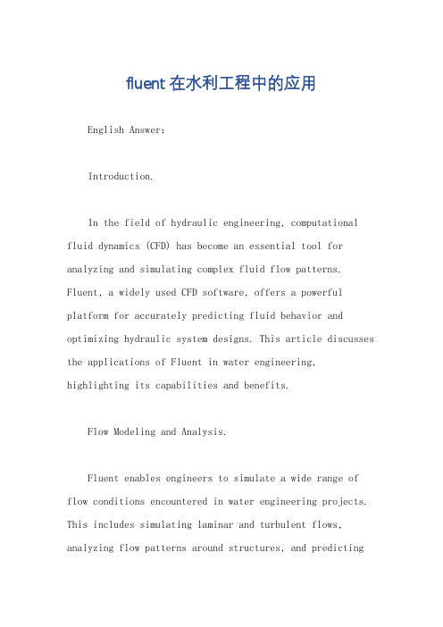
fluent在水利工程中的应用English Answer:Introduction.In the field of hydraulic engineering, computational fluid dynamics (CFD) has become an essential tool for analyzing and simulating complex fluid flow patterns. Fluent, a widely used CFD software, offers a powerful platform for accurately predicting fluid behavior and optimizing hydraulic system designs. This article discusses the applications of Fluent in water engineering, highlighting its capabilities and benefits.Flow Modeling and Analysis.Fluent enables engineers to simulate a wide range of flow conditions encountered in water engineering projects. This includes simulating laminar and turbulent flows, analyzing flow patterns around structures, and predictingwater quality parameters. By modeling flow in detail, engineers can gain insights into the behavior of water systems and identify potential issues.Sediment Transport Modeling.Sediment transport is a critical consideration in water engineering, as it affects the stability of riverbeds and channels. Fluent provides advanced capabilities for simulating sediment transport processes, allowing engineers to predict how sediment will behave under different flow conditions. This information is essential for designing erosion control measures and managing sediment accumulation.Hydropower Optimization.The design and operation of hydropower systems dependon accurate predictions of flow patterns and energy generation potential. Fluent can be used to simulate theflow of water through turbines and generators, assisting engineers in optimizing hydropower plant efficiency and maximizing power output.Water Quality Modeling.Water quality is a major concern in water engineering, and Fluent can be used to simulate the transport and dispersion of pollutants in water bodies. Engineers can use this capability to assess the impact of industrial discharges, predict pollutant concentrations, and design water treatment systems.Coastal Engineering.Coastal engineering involves the design and construction of structures and systems to protect coastlines from erosion and flooding. Fluent is used to simulate wave propagation, sediment transport, and coastal processes. This information is invaluable for designing effective coastal protection measures and mitigating the impact of natural disasters.Benefits of Using Fluent in Water Engineering.Accuracy: Fluent's advanced numerical algorithms provide accurate results for complex fluid flow problems.Versatility: Fluent can simulate a wide range of flow conditions and water engineering applications.User-Friendly Interface: Fluent's intuitive interface makes it accessible to engineers with varying levels of CFD experience.Time Savings: Fluent's powerful solvers significantly reduce simulation time compared to traditional methods.Cost Savings: By optimizing designs and minimizing potential issues, Fluent can ultimately lead to costsavings for water engineering projects.Conclusion.Fluent has become an essential tool in water engineering, providing engineers with the ability to accurately simulate and analyze complex fluid flow patterns.Its capabilities in flow modeling, sediment transport modeling, hydropower optimization, water quality modeling, and coastal engineering offer significant benefits for the design and operation of water systems. As the demand for efficient and sustainable water management solutions grows, Fluent will continue to play a vital role in advancing the field of water engineering.中文回答:前言。
Sediment Scour Model
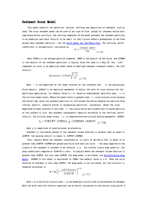
This model predicts the advection, erosion, settling and deposition of sediment, such as sand. The scour sediment model can be used in any type of flow, though all sediment motion must take place within one fluid. The settling component of the model presumes the sediment particles to be spherical and their velocity to be small (so that viscous effects predominate in the flow around each sediment particle)–see the Drift Model for Two-Phase Flow. The settling (drift)coefficient is automatically calculated asHere SCRDIA is the average particle diameter. RHOF is the density of the fluid, and SCRRHO is the density of the sediment particles; a typical value for sand is 2.65g/cm3. The “lift” component of scour is an empirical model based on Bed-Load sediment transport models; the lift velocityHere τ is the magnitude of the shear stresses at the interface and is the macroscopic fluid density. SCRALP is an empirical parameter to adjust the rate of scour erosion for the particular application. Its default value is 1.0, based on experimental data with sand. τ c is the critical shear stress. Where the shear stress is greater than τc, scour erosion occurs because the forces that cause the sediment particles to lift exceed the forces keeping the particle from lifting (gravity, cohesive forces to neighboring particles). Conversely, where the local magnitude of shear stresses is less than τc, the liquid forces are insufficient to causes particle at the surface to lift, and sediment subsequently deposits according to the settling (drift) velocity. The critical shear stress, τc, is computed from the critical Shields parameter, SCRCRT:Here g is magnitude of gravitational acceleration.Sediment is considered packed if the sediment volume fraction is greater than or equal to SCRFCR; the packing density is equal to SCRFCR×SCRRHO.Thus, regions where the sediment concentration (in units of gm/cm3 in CGS) is equal to or greater than SCRFCR×SCRRHO are packed and fluid flow does not occur –the drag imparted on the liquid by the sediment is assumed to be infinite (i.e., the inverse liquid drag quantity, the drag coefficient computed by FLOW-3D is zero). In regions where the sediment volume fraction is greater than SCRFCO, but less than SCRFCR, the drag model is activated (see Solidification Drag Model). SCRDRG in this model is equivalent to TSDRG (the default value is 1.0). When the solid fraction of sediment is less than SCRFCO, the drag model is not activated, but the viscosity is enhanced according to:Here μ0 is the fluid viscosity and μis the enhanced viscosity due to the presence of sediment. Both the drift and lift velocity equations can be easily customized in the routine scour_drift.f该模型预测泥沙的对流、侵蚀、沉降和淤积。
交通运输领域的主要SCI国际期刊

交通运输领域的主要SCI国际期刊IEEE TRANSACTIONS ON INTELLIGENT TRANSPORTATION SYSTEMS QuarterlyISSN: 1524-9050IEEE-INST ELECTRICAL ELECTRONICS ENGINEERS INC, 445 HOES LANE, PISCA TAWAY, USA, NJ, 08855ITE JOURNAL-INSTITUTE OF TRANSPORTATION ENGINEERSMonthlyISSN: 0162-8178INST TRANSPORTA TION ENGINEERS, 1099 14TH ST, NW, STE 300 WEST, W ASHINGTON, USA, DC, 20005-3438JOURNAL OF ADV ANCED TRANSPORTATIONTri-annualISSN: 0197-6729INST TRANSPORTA TION, STE 68, #305, 4625 V ARSITY DR, N W, CALGARY, CANADA, ALBERTA, T3A OZ9JOURNAL OF TRANSPORTATION ENGINEERING-ASCEBimonthlyISSN: 0733-947XASCE-AMER SOC CIVIL ENGINEERS, 1801 ALEXANDER BELL DR, RESTON, USA, V A, 20191-4400TRANSPORTATIONQuarterlyISSN: 0049-4488SPRINGER, 233 SPRING STREET, NEW YORK, USA, NY, 10013TRANSPORTATION JOURNALQuarterlyISSN: 0041-1612AMER SOC TRANSPORTA TION LOGISTICS, 1700 NORTH MOORE ST, STE 1900, ARLINGTON, USA, V A, 22209-1904TRANSPORTATION PLANNING AND TECHNOLOGYQuarterlyISSN: 0308-1060TAYLOR & FRANCIS LTD, 4 PARK SQUARE, MILTON PARK, ABINGDON, ENGLA ND, OXON, OX14 4RNTRANSPORTATION QUARTERLYQuarterlyISSN: 0278-9434ENO FOUNDATION TRANSPORT INC, 1634 I ST NW, STE 500, WASHINGTON, US A, DC, 20006-4003TRANSPORTATION RESEARCH PART A-POLICY AND PRACTICEMonthlyISSN: 0965-8564PERGAMON-ELSEVIER SCIENCE LTD, THE BOULEVARD, LANGFORD LANE, KID LINGTON, OXFORD, ENGLAND, OX5 1GBTRANSPORTATION RESEARCH PART B-METHODOLOGICALMonthlyISSN: 0191-2615PERGAMON-ELSEVIER SCIENCE LTD, THE BOULEVARD, LANGFORD LANE, KID LINGTON, OXFORD, ENGLAND, OX5 1GBTRANSPORTATION RESEARCH PART C-EMERGING TECHNOLOGIES BimonthlyISSN: 0968-090XPERGAMON-ELSEVIER SCIENCE LTD, THE BOULEVARD, LANGFORD LANE, KID LINGTON, OXFORD, ENGLAND, OX5 1GBTRANSPORTATION RESEARCH PART D-TRANSPORT AND ENVIRONMENT BimonthlyISSN: 1361-9209PERGAMON-ELSEVIER SCIENCE LTD, THE BOULEVARD, LANGFORD LANE, KID LINGTON, OXFORD, ENGLAND, OX5 1GBTRANSPORTATION RESEARCH PART E-LOGISTICS AND TRANSPORTATION REVIEWBimonthlyISSN: 1366-5545PERGAMON-ELSEVIER SCIENCE LTD, THE BOULEVARD, LANGFORD LANE, KID LINGTON, OXFORD, ENGLAND, OX5 1GBTRANSPORTATION RESEARCH PART F-TRAFFIC PSYCHOLOGY AND BEHAVI OURBimonthlyISSN: 1369-8478ELSEVIER SCI LTD, THE BOULEVARD, LANGFORD LANE, KIDLINGTON, OXFOR D, ENGLAND, OXON, OX5 1GBTRANSPORTATION RESEARCH RECORDISSN: 0361-1981NATL ACAD SCI, 2101 CONSTITUTION AVE, WASHINGTON, USA, DC, 20418TRANSPORTATION SCIENCEQuarterlyISSN: 0041-1655INST OPERATIONS RESEARCH MANAGEMENT SCIENCES, 901 ELKRIDGE LANDI NG RD, STE 400, LINTHICUM HTS, USA, MD, 21090-290961.交通运输类核心期刊表(33种)61.1综合运输类核心期刊表(10种)号刊名中文译名中图刊号出版国1IEEE transactions on vehiculartechnologyIEEE运载工具技术汇刊730B0001TVT美国2Transportation research.Part B,Methodological运输研究.B辑,方法论870C0066-2英国3Transportation research record运输研究记录870B0103美国4Transportation science运输科学870B0068美国5Transportation research.Part A,Policyand Practice运输研究.A辑,政策与实践870C0066-1英国6Transportation运输870LB052荷兰7Vehicle system dynamics车辆系统动力学873LB055荷兰8Journal of transportation engineering运输工程杂志860B0002-11美国9Transportation research.Part D,Transport and environment运输研究D辑,运输与环境870C00664英国10Transport reviews运输评论877C0144英国61.2铁路运输类核心期刊表(5种)号刊名中文译名中图刊号出版国1Proceedings Of the institution of Mechanical Engineerings.Part F,Journalof rail and rapid transit机械工程师学会会报.F辑,铁路与快速运输杂志780C0002-F英国2Railway gazette International国际铁路快报871C0058英国3Quarterly reports铁道技术研究所季报871D0070日本4Railway age铁路时代871B0004美国5 Rail international国际铁路871LA002比利时Urban transport sustainability--Asian trends, problems and policy practices61.3、公路运输类核心期刊表(9种)号刊名中文译名中图刊号出版国1International Journal of vehicle design国际机动车设计杂志873LD068瑞士2Journal of intelligent transportationsystems智能交通系统杂志873C0133英国3S.A.E.transactions汽车工程师学会汇刊870B0001美国4Journal of bridge engineering桥梁工程杂志860B0002-22美国5Heavy vehicle systems重型机动车系统873LD070瑞士6JSAE review日本汽车工程师学会评论873D0138日本7Traffic engineering&control交通工程与管理870C0064英国8Journal of terramechanlcs地面力学杂志873C0006英国9Public roads公路873B0007英国61.4、水路运输类核心期刊表(9种)序号刊名中文译名中图刊号出版国1Coastal engineering海岸工程875LB060荷兰2Journal of waterway,port,coastal,and oceanengineering航道、港口、海岸与海洋工程杂志860B0002-13美国3Journal of ship research船舶研究杂志875B0001美国4Naval engineers Journal航海工程师杂志875B0001美国5The Naval architect造船工程师875C0005英国6Marine structures海上构筑物875C0123英国7Marine technology and SNAME news船舶技术与SNAME新闻875B0071美国8International shipbuilding progress国际造船进展875LB001荷兰9Dredging +port construction疏浚与港口建设875C0087英国62.交通运输类扩展区期刊表(29种)62.1、综合运输类扩展区期刊表(9种)刊名中图刊号ISSN出版图ITE Journal870B00540162-8178美国Journal of Advanced Transportation870B00710197-6729英国Pipes and Pipelines International 874C00010032-020X英国Proceedings of the Institution of Civil Engineers.Transport860C0005-30965-092X英国Proceedings of the Institution of Mechanical Engineerings.Part D,Journal of Automobile Engineering780C0002-D0954-4070英国Public Transport International 870LA052A1029-1261比利时Transportation Planing and Technology870B0116美国Transportation Research。
北海和波罗的海三维业务海洋数值模拟和预报系统
❖ Where? The Suspendet Matter model is the collaborative development of the GkSS research center and the BSH (Gerhard Gayer et al. 2005).
❖ Processes? The regional circulation model (cmod) was extended by an Suspended Particulate Matter module to include vertical exchange processes (sedimentation, resuspension and erosion), bottom processes (consumption and bioturbation) and the horizontal redistribution of SPM due to currents and waves.
❖ First steps: Coupling of the GKSS-SPM model with the DMI circulation Model BSHcmod. Tests of the SPM-BSHcmod in the North Sea and Baltic Sea.
Whats done?
resuspension
u 0,01 m / s
u
erosion
0,028 m /
s
Bioturbation, diffusion
Z4 = 10cm
2. waves:
1 water column: SPM dynamic
2,08m
2,11m
0.000195 0.000361 0.000386 0.000410 0.000431 0.000447 0.000459 0.000467 0.000469 0.000466 0.000458 0.000447 0.000445
MODEL EVALUATION GUIDELINES FOR__ SYSTEMATIC

D. N. Moriasi, J. G. Arnold, M. W. Van Liew, R. L. Bingner, R. D. Harmel, T. L. Veith
Sensitivity analysis is the process of determining the rate of change in model output with respect to changes in model inputs (parameters). It is a necessary process to identify key parameters and parameter precision required for calibration (Ma et al., 2000). Model calibration is the process of estimating model parameters by comparing model predictions (output) for a given set of assumed conditions with observed data for the same conditions. Model validation involves running a model using input parameters measured or determined during the calibration process. According to Refsgaard (1997), model validation is the process of demonstrating that a given site-specific model is capable of making “sufficiently accurate” simulations, although “sufficiently accurate” can vary based on project goals. According to the U.S. EPA (2002), the process used to accept, reject, or qualify model results should be established and documented before beginning model evaluation. Although ASCE (1993) emphasized the need to clearly define model evaluation criteria, no commonly accepted guidance has been established, but specific statistics and performance ratings for their use have been developed and used for model evaluation (Donigian et al., 1983; Ramanarayanan et al., 1997; Gupta et al., 1999; Motovilov et al., 1999; Saleh et al., 2000; Santhi et al., 2001; Singh et al., 2004; Bracmort et al., 2006; Van Liew et al., 2007). However, these performance ratings are model and project specific. Standardized guidelines are needed to establish a common system for judging model performance and comparing various models (ASCE, 1993). Once established, these guidelines will assist modelers in preparing and reviewing quality assurance project plans for modeling (U.S. EPA, 2002) and will increase accountability and public a
Multigene genetic programming for sediment transpo
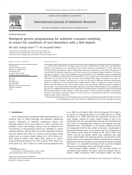
abstract
It is known that construction of large sewers based on consideration of flow with non-deposition without a bed deposit is not economical. Sewer design based on consideration of flow with nondeposition with a bed deposit reduces channel bed slope and construction cost in which the presence of a small depth of sediment deposition on the bed increases the sediment transport capacity of the flow. This paper suggests a new Pareto-optimal model developed by the multigene genetic programming (MGGP) technique to estimate particle Froude number (Frp) in large sewers with conditions of sediment deposition on the bed. To this end, four data sets including wide ranges of sediment size and concentration, deposit thickness, and pipe size are used. On the basis of different statistical performance indices, the efficiency of the proposed Pareto-optimal MGGP model is compared to those of the best MGGP model developed in the current study as well as the conventional regression models available in the literature. The results indicate the higher efficiency of the MGGP-based models for Frp estimation in the case of no additional deposition onto a bed with a sediment deposit. Inasmuch as the Pareto-optimal MGGP model utilizes a lower number of input parameters to yield comparatively higher performance than the conventional regression models, it can be used as a parsimonious model for self-cleansing design of large sewers in practice. & 2018 International Research and Training Centre on Erosion and Sedimentation/the World Association
hec-ras中文使用手册【word版】37p
_PC version first released in 1984于1984年第一次发布在网络上
_Last version 4.6.2 released in 1991于1991年发布了最后的版本4.6.2
_HEC “Next Generation” Software Development港口进入管制”下一代”软件开发
6
Entering Geometric Data进入几何数据
Draw the river asa schematic画出示意性的河道
Specify thecross sectiongeometry详细规定横截面几何
Cross Sectional Geometry截面几何
Reach Lengths流程的长度
_Computes floodplain encroachments估算漫滩侵蚀
_Models channel modifications模拟河渠修复
_Models bridge scour模拟桥梁冲刷
_Models flood control structures (ie. Dams) with inline weirsand gated spillways
_Version 3.1 released in January of 2003于2003年1月发布3.1版本
15
HEC-RAS—The Future and OtherConsiderations
港口进入管制-随机存取存储器—有关远景和其他方面的考虑
_Importance of HEC-RAS港口进入管制-随机存取存储器的重要性
_ASK QUESTIONS PLEASE!请提问
Identifying Transportation Modes from Raw GPS Data
Identifying Transportation Modes from Raw GPSDataQiuhui Zhu;Min Zhu;Mingzhao Li;Min Fu;Zhibiao Huang;Qihong Gan;Zhenghao Zhou 【期刊名称】《国际计算机前沿大会会议论文集》【年(卷),期】2016(000)001【摘要】Raw Global Positioning System (GPS) data can provide rich context information for behaviour understanding and transport planning. However, they are not yet fully understood, and fine-grained identification of transportation mode is required. In this paper, we present a robust framework without geographic information, which can effectively and automatically identify transportation modes including car, bus, bike and walk. Firstly, a trajectory segmentation algorithm is designed to divide raw GPS trajectory into single mode segments. Secondly, several modern features are proposed which are more discriminating than traditional features. At last, an additional postprocessing procedure is adopted with considering the wholeness of trajectory. Based on Random Forest classifier, our framework can achieve a promising accuracy by distance of 82.85% for identifying transportation modes and especially 91.44% for car mode.【总页数】3页(P100-102)【作者】Qiuhui Zhu;Min Zhu;Mingzhao Li;Min Fu;Zhibiao Huang;Qihong Gan;Zhenghao Zhou【作者单位】[1]College of Computer Science,SichuanUniversity,Chengdu,China;[1]College of Computer Science,Sichuan University,Chengdu,China;[2]RMITUniversity,Melbourne,Australia;[1]College of Computer Science,Sichuan University,Chengdu,China;[3]Chengdu Institute of Computer Application,Chinese Academy of Sciences,Chengdu,China;[4]Modern Education Technology Center,Sichuan University,Chengdu,China;[5]High School No.7,Chengdu,China【正文语种】中文【中图分类】C5【相关文献】1.An Enhanced Transportation Mode Detection Method Based on GPS Data [J], Jing Liang;Qiuhui Zhu;Min Zhu;Mingzhao Li;Xiaowei Li;Jianhua Wang;Silan You;Yilan Zhang;2.Data Envelopment Analysis Model for Assessment of Safety and Security of Intermodal Transportation Facilities [J], Evangelos I.Kaisar; Ramesh Teegavarapu; Elisabeth Gundersen3.Determination of groundwater solute transport parameters in finite element modelling using tracer injection and withdrawal testing data [J], Van Hoang Nguyen4.Artificial neural network model for identifying taxi gross emitter from remote sensing data of vehicle emission [J], ZENG Jun;GUO Hua-fang;HU Yue-ming5.Identifying who best tolerates moderate sedation:Results from a national database of gastrointestinal endoscopic outcomes [J], Monica Passi;Farial Rahman;Sandeep Gurram;Sheila Kumar;Christopher Koh因版权原因,仅展示原文概要,查看原文内容请购买。
sediment-transport1
4. Sediment Transport •Introduction•Properties of sand•Threshold of motion•Bed features•Suspended sediment•Bedload transport•Total load transport •Applications4.1 INTRODUCTION•Coastal engineering applications–Beach erosion and erosion control•Interaction of sediment transport with human activities andman made structures–Deposition of sediments in harbour or navigationchannels–Local scour around coastal structures •Offshore engineering applications–Scour around offshore structures & pipelines–Backfill of pipeline trenchesWaves/Sediment/StructureInteractionsSeawall with frontal protection, Initially, but some years later …Erosion and Erosion ControlOarai Harbor, Japan1988 1976Oarai 1976, 1988What to Study?•Sediment properties•Wave and flow forcing mechanisms •Interaction of flow and sediments –Threshold of motion for sediments–Sediment responses to different flowconditions•Transport rates•Seabed deformations–Consequences of sediment transportDefinition of Seabed ShearStressShear stress measures: (1) shear stress t 0(N/m 2); (2) friction velocity u *(m/s)2*0u r t =(4.1)Dimensionless form of bed shear stress: Shields parameter q()()d s g u d g s 12*0-=-=r r t q (4.2)Where r s is the density of the sediment and s (=r s /r ) is the specific density.The total bed shear stress on the bed is comprised of the following components:•The skin friction t 0s produced by the sand grains •The form drag t 0f produced by the pressure field associated with the flow over ripples •The sediment-transport contribution t 0t caused by momentum transfer to themobile grains.4.2 Properties of Sediments•Classification–Based on sedimentgrain sizes;–Clays, silts, sands,gradules, pebbles andboulders–Geologists use fscales: f = log2d,where d is the graindiameter in mmWentworth ScaleSize Analysis•Seabed sedimentsare non-uniform–Particle sizedistribution ispresented ascumulative percentageby mass smaller thand;–Spread of sizes isindicated by thegeometric standard deviation: 1684/d d g =sProperties of Sand-WaterMixturesProperties of Sand-Water Mixtures4.3 Threshold of Motion•Threshold of motion (incipient motion)–Defined as the critical bed shear stress orcritical velocity beyond which significantamount of grains begin to move–Threshold of motion for non-cohesivesediments on a horizontal bed can beevaluated from Shields diagramThreshold Current SpeedThe following threshold depth-averaged speed on a flat, horizontal, un-rippled bed has been proposed by van Rijn (1994) for fresh water at 15o C, r s = 2650 kg/m 3and g = 9.81 m/s 2:()()90101.050/4log 19.0d h d U cr =(4.3)Where h is the water depth.for 100 ≤ d 50≤ 500 m m()()90106.050/4log 5.8d h d U cr =(4.4)for 500 ≤ d 50≤ 2000 m m A more general formula proposed by Soulsby (1997) reads[]2/1*507/150)()1(7D f d s g d h U cr -⎪⎪⎭⎫ ⎝⎛=for D *> 0.1(4.5)with [])020.0exp(1055.02.1130.0)(***D D D f --++=(4.6)Where503/12*)1(d s g D ⎥⎦⎤⎢⎣⎡-=νExample 4.1Calculate the threshold depth-averaged current speed for steady flow over a flat sand bed with the following characteristics:d 50= 200 m m, d90= 300 m m, h = 5 m, r= 1027 kg/m3, ν= 1.36⨯10-6m2/sr s= 2650 kg/m3.Threshold Wave Orbital VelocityThe threshold orbital velocity under waves can be calculated using Komar and Miller (1974) formula:[]3/13/13/2)1(118.0T d s g U cr -=for d < 0.5 mm (4.7)[]7/17/37/4)1(09.1T d s g U cr -=for d > 0.5 mm (4.8)Eqs. (4.7) and (4.8) are widely used but have the disadvantage of having a large discontinuity at d = 0.5 mm.•The threshold orbital velocity under waves can also be calculated using the critical shear stress approach.Example 4.2Calculate the threshold orbital velocity for monochromatic wave passing over a flat sand bed with the following characteristicsd 50= 200 m m, T = 8s, r= 1027 kg/m3, rs= 2650 kg/m3.The best fit of the data given in the diagram on next slide was proposed by Soulsby (1997)[])020.0exp(1055.02.1130.0**D D cr --++=q (4.11)d s g D 3/12*)1(⎥⎦⎤⎢⎣⎡-=νThreshold Shear StressA more precise measure of the threshold of motion is the bed shear stress approach developed by Shields (1936) in terms of the ratio of the bed shear force to the submerged weight of a grain on the bed. The threshold Shields parameter is defined as()d g s cr cr r r t q -=(4.9)t cr is the threshold bed shear-stress, r s is the grain density, r is water density and d is the grain diameter.The experimental data on the threshold Shields parameter is given in the next slide. In the figure:(4.10)Shields DiagramCritical Shear StressExample 4.3Calculate the threshold shear stress for sediment and sea water with following propertiesd 50= 200 m m, r= 1027 kg/m3, rs= 2650 kg/m3, ν= 1.36⨯10-6 m2/sThreshold Grain Diameter For steady currents[]4.14.08.2)1(25.0-=s g h U d cr (TGD -1)for d cr >10 mm For waves[]08.208.108.3)1(9.97-=s g T U d w cr (TGD -2)for d cr >10 mm Where d cr = threshold grain diameter; Ū = Depth -averaged current speed;h = water depth; U w = wave orbital velocity amplitude at the seabed;T = period of water wave; s = specific gravity of sediment grain;g = acceleration due to gravityExample 4.4In a combined wave and current flow, the peak bed shear-stress has been estimated to be 2.0 N/m2. What size of sand or gravel will be stable in this flow. Assumer= 1027 kg/m3, r s= 2650 kg/m3, ν= 1.36⨯10-6 m2/sThreshold Conditions on a SlopingBed βFlow βFlow(a)(b)βy(c))sin()sin(i i cr cr f βf t t β+=βf βt t βcos ])(tan )(tan 1[2/122i cr cr -=)tan(sin sin tan cos sin cos 2222i i cr cr f βy f ββy t t β-+=Example 4.5Calculate the threshold shear stress for sediment and sea water with following properties on a bed slope at 20o. Assume the current flowing at an angle of 45o to the upslope direction.d 50= 200 m m, r= 1027 kg/m3, rs= 2650 kg/m3, ν= 1.36⨯10-6m2/sSeabed Shear Stress Induced bySteady Currents•Bed shear stress is the frictional force exerted on unit area bed by current flowing over it;•Bed shear stress is the major forcing mechanism for sediment transport;•Bed shear stress is dependent on flow velocity, viscosity, roughness, bed forms and boundary layer thicknessSteady Current Profile•Currents in the sea may be caused by tidal motions, wind-stress, etc..•Wave-induced currents dominate in the near shore region and a combination of tidal and meteorological forcing dominates further offshore•Turbulent boundary layers in ocean are typically some meters or tens of meters thick•The definition of depth-averaged current speed:⎰=h dz z U h U 0)(1(4.12)•Within the bottom few meters above the seabed the current velocity varies with the height z above the bed according to the logarithmic velocity profile)ln()(0*z z u z U κ=(4.13)Where z 0is the bed roughness height, k is von Karman’s constant ( = 0.41) and u *is the friction velocity.•Eq. (4.13) is valid from a few centimetres above the bed up to 20-30% of the water depth in shallow water (2-3 m), or 20-30% of the boundary-layer thickness in deep water (20-30m).•Nikuradse’s (1933) experiments indicated that the bed roughness height z 0depends on the viscosity of the water, the current speed and the dimensions of the physical roughness of the bed•A good fit to the experimental results of Nikuradse is given by Christoffersen and Jonsson (1985):**0927exp 130u k u k z S S νν+⎥⎦⎤⎢⎣⎡⎪⎭⎫ ⎝⎛--=(4.14)Where νis the viscosity of the water and k s is the Nikuradse’s roughness. There have been many empirical formulae on relationship between k s and grain diameter.A widely used relationship between k s and grain diameter is:505.2d k S =(4.15)There are other ways to define k s using grain diameters. These will not be listed here. In reality, the seabed often comprises of mixed sediments and is non-flat. The Table given on next slide lists typical values of z 0for different natural seabeds.The tidal current velocity profile throughout the water column is given with reasonable accuracy by (Soulsby 1990):hz z z U z U 2/)2/ln()/ln()(00δδ-=h z z z U z U 2/)2/ln()2/ln()(00δδ-=for z 0< z < 0.5δ(4.16)for 0.5δ< z < h (4.17)Where Ū is the depth-averaged current speed, h is the water depth and δis the boundary-layer thickness.Tidal boundary-layer thickness can be estimated using (Soulsby 1983):⎪⎪⎭⎫ ⎝⎛--=220038.0f f U U b a s s δWhere: s = the radian tidal frequency (e.g. s = 1.4052⨯10-4rad/s for the M2 (semidiurnal) tide)f = 1.4544⨯10-4⨯sin (latitude) rad/s is the Coriolis parameter.Ūa and Ūb = maximum and minimum values of the depth-averaged current speed during a tidal cycle.(4.18)The tidal current can also be estimated using an empirical formula due to Soulsby (1990):U h z z U 7/132.0)(⎪⎭⎫ ⎝⎛=U z U 07.1)(=for 0 < z < 0.5h (4.19)for 0.5h < z < h (4.20)A question:how do we get depth-averaged velocity from measurement of a velocity profile?Measurement points (increasing upwards): (z 1, U 1), (z 2, U 2), …… (z n , U n ))](2))((..))(([5.0)(11122111n n n n n n z h U z z U U z z U U z U hz U -+-+++-++=--Conditions:(a) Sufficient points covering wide range of heights; (b) z 1is close enough to the seabed; (c) z n > h/2; (d) measurements are either simultaneous or short enough for significant flow changesCalculate the velocity at a height of 2 m above a flat bed of sand of uniform diameter d = 200 m m, if the bed shear-stress is 0.2 N/m2and the water density is 1027 kg/m3.Calculate the velocity at a height of 1 m above a flat bed and the surface velocity, in water of depth 20 m when the depth-averaged velocity is 0.5 m/s.Current Skin-Friction Shear Stress •The bed shear-stress is defined as the frictional force acting on unit area of seabed by the current flowing over it•The total shear stress equals approximately to the skin-friction if the seabed is flat with no ripples and sediment transport is not very intensive•The bed shear-stress is related to the depth-averaged current speed Ū through a drag coefficient as:20U C D r t =(4.21)Where C D can be related to the Darcy-Weisbach resistance coefficient, the Ch ézy coefficient C and Manning-Strickler coefficient n as:h gn C g f C D 228===(4.22)Where h is water depth and g is the acceleration due to gravity.The friction velocity is defined as:r t /0*=u (4.23)The value of C D can be determined in terms of the bed roughness through a simple power law formula:βα⎪⎭⎫ ⎝⎛=h z C D 0(4.24)WhereManning-Strickler law: α= 0.0474 and β= 1/3Dawson et al (1983): α= 0.0190 and β= 0.208Experimental data:Curve-fitting of the experimental data suggests:7/150*71⎪⎭⎫ ⎝⎛=h d U u (4.25)Substituting z 0= d 50/12 into Eq (4.25) yields: α= 0.0415 and β= 2/7. Thesevalues of the coefficients are recommended (Soulsby 1997) in preference to the coefficients of Manning-Strickler and Dawson et al..Eq. (4.25) is compatible with the power-law velocity distribution given by Eq. (4.19):)(121.07/150*z U z d u ⎪⎭⎫ ⎝⎛=(4.26)Where U(z) could be a measured velocity at a height z close to the bed.Alternatively, a logarithmic relationship can also be used:20)/ln(⎥⎦⎤⎢⎣⎡+=h z B C D κ(4.27)WhereB = 1 and κ= 0.4 if Eq. (4.13) is used throughout the water depthB = (δ/2h)-ln(δ/2h) and κ= 0.4 if Eq. (4.16) is used throughout the water depthComments:•The choice of methods in practice depends on the type of application•The logarithmic form of equation (Eq. (4.27)) has the strongest physical justification but the power-law form of equation (e.g. Eq. (4.24)) is more convenient formathematical manipulation. Both types of equations are equally well supported by data•Where no information is available or only a rough estimate is needed, a default value of C D = 0.0025 can be taken.•For flows with a complex variation in the vertical direction or in time can be estimated using21001000U C r t =(4.28)Where U 100is the current speed at a height of 1 m above the bed and C 100is the drag coefficient given in Table 7.Example 4.8Calculate the skin friction if the depth-averaged velocity is 1.0 m/s in water depth of 5 m, the sediment diameter is d50= 1 mm, and the density of water is 1027kg/m3.Current Total Shear Stress•The most common condition outside the surf zone in the sea is that the seabed is formed into ripples, dunes or sand waves•With limited sediment transport the total bed shear-stress t 0is composed of two components: the skin friction t 0s due to the drag on individual grains and the form drag component t 0f due to the pressure field acting on ripples or larger bedforms:fs 000t t t +=(4.29)•The typical ratio of t 0/t 0s is in the range of 2 –10 for a rippled bed •Only t 0s is responsible for transporting sand grains. But t 0f contributes to start the grains.•Only limited knowledge available on the methods of calculating t 0f . However the total shear stress can be calculated by assigning a total roughness length z 0(e.g. Table 7).•At very high flow speeds with intense sheet flow, a third component of the total shear-stress arises from sand grain interactions. This is called sediment transport shear-stress.•The calculation of sediment transport shear-stress is often incorporated in calculating total shear-stress through the total roughness length. The sediment transport roughness length can be calculated in terms skin friction as:)(30500r r t -=s s t g z (4.30)•Total roughness length can be calculated using:t f s z z z z 0000++=(4.31)•Due to the nonlinear nature of the equations, the total shear stress calculated using the total roughness length will be different from the value obtained bycomputing the three separate components and then summing. The total roughness length approach should be used.Calculate the bed shear-stress acting on an area of seabed above which measurements with current meters at heights of z = 0.1, 0.5, 1.0 and 2.0 m above the seabed, averaged over 10 minutes, were found to give U(z) = 0.2, 0.34, 0.37 and 0.45 m/s, respectively.Calculate the bed shear-stress acting on an area of rippled sand seabed above which a current meter mounted at a height of 1m gives an average speed over 10 = 0.5 m/s.min of U100Wave Skin-Friction Shear-Stress •The seabed shear stress produced by the orbital velocity U w can be obtained via the wave friction factor, f w , as:221w w w U f r t =(4.32)•On a flat seabed with no ripples, the wave friction factor depends on the flow regime (laminar, smooth turbulent, or rough turbulent), which in turn is dependent on the wave Reynolds number Rw and the relative roughness r:νAU R w w =(4.33)s k A r =(4.34)Where U w = bottom orbital velocity amplitude; A = U w T/2p ; T = wave period;ν= kinematic viscosity; k s = Nikuradse equivalent sand grain roughnessMyrhaug (1989) gives an implicit relationship for f w , which is valid for smooth, transitional and rough turbulent flows:64.171.40262.0exp(1ln )36.6ln(32.022/12/12/1+⎭⎬⎫⎩⎨⎧+⎥⎦⎤⎢⎣⎡---=w w w w w w f R r r f R rf f (4.35)For rough turbulent flow, Soulsby (1997) proposed that52.0273.0-=r f wr (4.36)for all rNw ws BR f -=(4.37)for smooth bedWhereB = 2, N = 0.5 for R w ≤ 5⨯105(laminar)B = 0.0521, N = 0.187 for R w > 5⨯105(smooth turbulent)A Note on the Use of Uw •Linear wave theory can be used to calculate Uw for monochromatic waves •For spectrum waves, two approximations available:e linear wave theory throughapproximations of H = H rms=H s/1.414 and T= T pe a spectrum: Uw = 1.414U rms and T = T pWave Total Shear-Stress •Total shear-stress = skin-friction + form drag component + sediment transport component•Form drag component is due to bed forms such as ripples and dunes•Calculation of form drag and sediment transport components are rather difficult and is achieved through a total roughness length.Example 4.11Calculate the wave skin friction on a smooth seabed of sand with d50= 0.48 mm,subject to H s= 3 m waves with zero crossing wave period of T z= 8 s in 10 m water.Wave and Current Combined Skin-Friction Shear Stress•Wave and current combined behaviour in sediment transport is not a linear sum of their separate behaviours due to the current and wave interactions such as:–Modification of the phase speed and wave length of waves by the current, leading to refraction of the waves–Interaction of the wave and current boundary layers, leading to enhancement of both the steady and oscillatory components of thebed shear-stress–Generation of currents by the waves, including longshore currents, undertow, and mass transport currents.•The dispersion relation for waves in the presence of a depth-averaged current of speed Ūat an angle f to the direction of wave travel is())ω(4.38)-fU=cos2khtanh(gkkBed Shear-Stress•Non-linear interactions between wave and current boundary layers make the prediction of total bed shear-stress very difficult•The bed shear-stress due to wave and current combined can be larger than the values that would result from a simple linear addition of the wave-alone and current-alone stresses•More than 20 different theories and models have been proposed. The difference between these models are generally about 30-40% but could be up to a factor of 3 for strongly wave-dominated conditions•A comparison of between predictions of the mean ( t m) and maximum bed shear stress during a wave cycle by 8 models is given in the figure on next slides。
核质转运(zuixin)
Transport of macromolecules between the nucleus and cytoplasm is a critical cellular process for eukaryotes, and the machinery that mediates nucleocytoplasmic exchange is subject to multiple levels of control.
mRNA:Specific proteins are cotranscriptionally
recruited to form a messenger ribonucleoprotein particle (mRNP) with serial changes to the mRNP during splicing, capping, and polyadenylation. Regulated mRNP maturation is required for export, with deficiencies resulting in nuclear mRNP retention.
Cargo signals: NF-κB and p53
Fig.(A) Intermolecular and intramolecular interactions (NF-kB or p53, respectively) regulate trafficking of single cargoes.
Ubiquitination(泛素化): The ubiquitin-conjugating
enzyme UbcM2 is imported only when charged with ubiquitin, implicating proper enzyme activation as a transport “trigger”.
- 1、下载文档前请自行甄别文档内容的完整性,平台不提供额外的编辑、内容补充、找答案等附加服务。
- 2、"仅部分预览"的文档,不可在线预览部分如存在完整性等问题,可反馈申请退款(可完整预览的文档不适用该条件!)。
- 3、如文档侵犯您的权益,请联系客服反馈,我们会尽快为您处理(人工客服工作时间:9:00-18:30)。
Sediment Transport Modeling Review—Current andFuture DevelopmentsAthanasios N.͑Thanos ͒PapanicolaouAssociate Professor,Univ.of Iowa,IIHR-Hydroscience and Engineering,Dept.of Civil and Environmental Engineering,Iowa City,IA 52241.E-mail:apapanic@Mohamed ElhakeemResearch Associate Engineer,Univ.of Iowa,IIHR-Hydroscience and En-gineering,Dept.of Civil and Environmental Engineering,Iowa City,IA 52241.E-mail:melhakee@George KrallisERM Inc.,Exton,PA.E-mail:george.krallis@Shwet PrakashERM Inc.,Exton,PAJohn EdingerFaculty Research Associate,Bryn Mawr College,Dept.of Geology.E-mail:jeedgr@IntroductionThe use of computational models for solving sediment transport and fate problems is relatively recent compared with the use of physical models.Several considerations govern the choice be-tween physical and computational models;namely,the nature of the problem that needs to be solved,the available resources,and the overall cost associated with the problem solution.In some specific problems,a combination of physical and computational models can be used to obtain a better understanding of the pro-cesses under investigation ͑de Vries 1973͒.Using computational hydrodynamic/sediment transport models,in general,involves the numerical solution of one or more of the governing differential equations of continuity,momentum,and energy of fluid,along with the differential equation for sediment continuity.An advan-tage of computational models is that they can be adapted to dif-ferent physical domains more easily than physical models,which are typically constructed to represent site-specific conditions.An-other advantage of computational models is that they are not sub-ject to distortion effects of physical models when a solution can be obtained for the same flow conditions ͑identical Reynolds and Froude numbers,same length scale in the three directions,etc.͒as those present in the field.With the rapid developments in numerical methods for fluid mechanics,computational modeling has become an attractive tool for studying flow/sediment transport and associated pollutant fate processes in such different environments as rivers,lakes,and coastal areas.Representative processes in these environments in-clude bed aggradation and degradation,bank failure,local scour around structures,formation of river bends,fining,coarsening and armoring of streambeds,transport of point source and nonpointsource pollutant attached to sediments,such sediment exchange processes as settling,deposition,and self-weight consolidation;coastal sedimentation;and beach processes under tidal currents and wave action.Over the past three decades,a large number of computational hydrodynamic/sediment transport models have been developed ͑Fan 1988;Rodi 2006͒.Extensive reviews of different hydrodynamic/sediment transport models can be found in Nicollet ͑1988͒,Nakato ͑1989͒,Onishi ͑1994͒,Przedwojski et al.͑1995͒,Spasojevic and Holly ͑2000͒,and the ASCE Sedimentation Engi-neering Manual no.110͑2007͒.Broadly speaking,these models can be classified on the basis of the range of their applications ͑e.g.,suspended load versus bed-load;physical versus chemical transport ͒;and their formulation in the spatial and temporal con-tinua ͑e.g.,one-dimensional model ͑1D ͒;two-dimensional model ͑2D ͒;or three-dimensional model ͑3D ͒;and steady versus un-steady ͒.The choice of a certain model for solving a specific prob-lem depends on the nature and complexity of the problem itself,the chosen model capabilities to simulate the problem adequately,data availability for model calibration,data availability for model verification,and overall available time and budget for solving the problem.The objectives of this article are twofold.First,the article aims to trace the developmental stages of current representative ͑1D,2D,and 3D ͒models and describe their main applications,strengths,and limitations.The article is intended as a first guide to readers interested in immersing themselves in modeling and at the same time sets the stage for discussing current limitations and future needs.Second,the article provides insight about future trends and needs with respect to hydrodynamic/sediment transport models.In preparing this article,the authors may have uninten-tionally omitted some models,since including all the available models found in the literature is impossible.Finally,this article is mainly focused on multidimensional computational models ͑2D and 3D models ͒;however,a brief overview of the 1D models is also included for providing a rational comparison of the 1D model features with the main features of the 2D and 3D models.Description of ModelsThis section provides information about the model formulation,the spatial and temporal characteristics,the coupling/linkage of the hydrodynamic and sediment components,and the model’s predictive capabilities.Tables 1–3complement this description by providing useful information about the model capabilities to handle unsteady flows,bed load and suspended load,sediment exchange processes,type of sediment ͑cohesive versus cohesion-less ͒,and multifractional sediment rmation about model acronyms,language,availability,and distribution is also provided in Tables 1–3.Tables 4–6summarize examples of the different model applications.The reader can use these case stud-JOURNAL OF HYDRAULIC ENGINEERING ©ASCE /JANUARY 2008/1D o w n l o a d e d f r o m a s c e l i b r a r y .o r g b y Z h e j i a n g U n i v e r s i t y o n 01/26/13. C o p y r i g h t A S CE .F o r p e r s o n a l u s e o n l y ; a l l r i g h t s r e s e r v e d .ies as a reference guide for model setup,calibration,and verifi-cation.One-Dimensional ModelsSince the early 1980s,1D models have been used with some success in research and engineering practice.Most of the 1D models are formulated in a rectilinear coordinate system and solve the differential conservation equations of mass and momen-tum of flow ͑the St.Venant flow equations ͒along with the sedi-ment mass continuity equation ͑the Exner equation ͒by using finite-difference schemes.Some representative models that are developed on the basis of the previously mentioned equations include MOBED by Krishnappan ͑1981͒,IALLUVIAL by Karim and Kennedy ͑1982͒,CHARIMA by Holly et al.͑1990͒,SEDI-COUP by Holly and Rahuel ͑1990͒,3ST1D by Papanicolaou et al.͑2004͒.The HEC-6formulation by Thomas and Prashum ͑1977͒is also presented in a rectilinear coordinate and is dis-cretized by using finite-difference schemes;but it solves the differential conservation equation of energy instead of the mo-mentum equation.Among other 1D models that use different coordinate systems,equations or schemes of solution are FLUVIAL 11by Chang ͑1984͒,GSTARS by Molinas and Yang ͑1986͒,and OTIS by Runkel and Broshears ͑1991͒.Chang ͑1984͒used a curvilinear coordinate system to solve the governing equations of his model.Molinas and Yang ͑1986͒implemented the theory of minimum stream power to determine the optimum channel width and ge-ometry for a given set of hydraulic and sediment conditions.Runkel and Broshears ͑1991͒modified the 1D advection-diffusion equation with additional terms to account for lateral inflow,first-order decay,sorption of nonconservative solutes,and transient storage of these solutes.Most of the 1D models that are presented here can predict the basic parameters of a particular channel,including the bulk-velocity,water surface elevation,bed-elevation variation,and sediment transport load.All of them,except OTIS,can also pre-dict the total sediment load and grain size distribution of nonuni-form sediment.3ST1D by Papanicolaou et al.͑2004͒cannot differentiate the total sediment load into bed load and suspended load.HEC-6by Thomas and Prashum ͑1977͒and IALLUVIAL by Karim and Kennedy ͑1982͒are not applicable to unsteady flow conditions.Table 1contains the complete model reference and acronym explanation and summarizes the main features for each model.Some of these 1D models have additional specific features.HEC-6by Thomas and Prashum ͑1977͒,for example,decom-poses energy losses into form loss and skin friction loss.MOBED by Krishnappan ͑1981͒can predict the sediment characteristics of a streambed as a function of time and distance for different flow hydrographs.FLUVIAL 11by Chang ͑1984͒accounts for the presence of secondary currents in a curved channel by adjusting the magnitude of the streamwise velocity.The same model can predict changes in the channel bed profile,width,and lateral mi-gration in channel bends.CHARIMA by Holly et al.͑1990͒andHEC-6:Hydraulic Engineering Center;Thomas and Prashum ͑1977͒V .4.2͑2004͒Steady Yes Yes Yes No Entrainment and deposition PDPDF77MOBED:MObile BED;Krishnappan ͑1981͒—Unsteady Yes Yes Yes No Entrainment and deposition C C F90IALLUVIAL:Iowa ALLUVIAL;Karim and Kennedy ͑1982͒—Quasi-steady Yes Yes Yes No Entrainment and deposition C C FIV FLUVIAL 11;Chang ͑1984͒—Unsteady Yes Yes Yes No Entrainment and deposition C P FIV GSTARS:Generalized sediment transport models for alluvial River simulation͑Molinas and Yang,1986͒V .3͑2002͒Unsteady Yes Yes Yes No Entrainment and deposition PDPDF90/95CHARIMA:Acronym of the word CHARiage which means bedload in FrenchHolly et al.͑1990͒—Unsteady Yes Yes Yes Yes Entrainment and deposition C C F 77SEDICOUP:SEDIment COUPled;Holly and Rahuel ͑1990͒—Unsteady Yes Yes Yes No Entrainment and deposition C C F77OTIS:One-dimensional transport with inflow and storage;Runkel and Broshears ͑1991͒V .OTIS-P ͑1998͒Unsteady No Yes No No Advection-diffusion PDPDF 77EFDC1D:Environmental fluid dynamics code;Hamrick ͑2001͒—Unsteady Yes Yes Yes Yes Entrainment anddeposition PD PD F773STD1,steep stream sediment Transport 1D model;Papanicolaou et al.͑2004͒—Unsteady a Yes aYes Yes No Entrainmentand deposition C P F90Note:V ϭversion;C ϭcopyrighted;LD ϭlimited distribution;P ϭproprietary;PD ϭpublic domain;and F ϭFORTRAN.aTreated as a total load without separation.2/JOURNAL OF HYDRAULIC ENGINEERING ©ASCE /JANUARY 2008D o w n l o a d e d f r o m a s c e l i b r a r y .o r g b y Z h e j i a n g U n i v e r s i t y o n 01/26/13. C o p y r i g h t A S CE .F o r p e r s o n a l u s e o n l y ; a l l r i g h t s r e s e r v e d .OTIS by Runkel and Broshears ͑1991͒can treat transport and fate of conservative contaminants and heat.EFDC1D by Hamrick ͑2001͒can be applied to stream networks.3ST1D by Papanico-laou et al.͑2004͒is capable of capturing hydraulic jumps and simulating supercritical flows;therefore,it is applicable to un-steady flow conditions that occur over transcritical flow stream reaches,such as flows over step-pool sequences in mountain streams.Because of their low data,central processor unit ͑CPU ͒re-quirements,and simplicity of use,1D models remain useful pre-dictive tools even today,especially in consulting,for rivers and stream ecological applications where 2D or 3D models may not be needed and are computationally expensive.Table 4presents examples of different 1D model applications.Two-Dimensional ModelsSince the early 1990s,there has been a shift in computational research toward 2D models.Most of the 2D models are currently available to the hydraulic engineering community as interface-based software to allow easy data input and visualization of re-sults.This added capability has made these models user-friendly and popular.2D models are depth-averaged models that can pro-vide spatially varied information about water depth and bed elevation within rivers,lakes,and estuaries,as well as the mag-nitude of depth-averaged streamwise and transverse velocity com-ponents.Most 2-D models solve the depth-averaged continuity and Navier-Stokes equations along with the sediment mass bal-ance equation with the methods of finite difference,finite element,or finite volume.Table 2shows the complete model reference and explanation of the model acronym and summarizes the characteristics of selected 2D hydrodynamic/sediment trans-port models.The main specific features of each model are de-scribed below:SERATRA:A finite-element sediment-contaminant transport model developed by Onishi and Wise ͑1982͒.The model includes general advection-diffusion equations and incorporates sink/source terms.The model can predict overland ͑terrestrial ͒and in-stream pesticide migration and fate to assess the potential short-and long-term impacts on aquatic biota in receiving streams.SUTRENCH-2D:A finite-volume hydrodynamic and sediment transport model developed by van Rijn and Tan ͑1985͒for simu-SERATRA:SEdiment and RAdionuclide TRAnsport;Onishi and Wise ͑1982͒—Unsteadya Yes a Yes No Yes Advection-diffusion CC/LDFIVSUTRENCH-2D:SUspended sediment transport in TRENCHes;van Rijn and Tan ͑1985͒—Quasisteadya Yes a Yes No No Advection-diffusion C LD F90TABS-2;Thomas and McAnally ͑1985͒—Unsteadya Yes a Yes No Yes Entrainment and deposition C C F77MOBED2:MObile BED;Spasojevic and Holly ͑1990a ͒—Unsteady Yes Yes Yes No Entrainment and depositionC C F77ADCIRC:ADvanced CIRCulation;Luettich et al.͑1992͒—Unsteady a Yes aYes No Yes Advection-diffusionC/LD C/LD F90MIKE 21:Danish acronym of the word microcomputer;Danish Hydraulic Institute ͑1993͒—Unsteady a Yes aYes No Yes Entrainment and deposition CPF90UNIBEST-TC:UNIform BEach Sediment Transport—Transport Cross-shore;Bosboom et al.͑1997͒—Quasi-steadya Yes a Yes No No Entrainment and advection C LD F90USTARS:Unsteady Sediment Transport models for Alluvial Rivers Simulations;Lee et al.͑1997͒—Unsteady Yes Yes Yes No Entrainment and deposition P P F90FAST2D:Flow Analysis Simulation Tool;Minh Duc et al.͑1998͒—Unsteady Yes Yes No No Entrainment and deposition LD P F90FLUVIAL 12;Chang ͑1998͒—Unsteady Yes Yes Yes No Entrainment and deposition C P F77Delft 2D;Walstra et al.͑1998͒—Unsteady Yes Yes No Yes Advection-diffusion C LD F90CCHE2D:The National Center for Computational Hydroscience and Engineering;Jia and Wang ͑1999͒V .2.1͑2001͒Unsteady Yes Yes Yes No Advection-diffusion PD/CLDF77/F90Note:V ϭversion;C ϭcopyrighted;LD ϭlimited distribution;P ϭproprietary;PD ϭpublic domain;F ϭFORTRAN.aTreated as a total load without separation.JOURNAL OF HYDRAULIC ENGINEERING ©ASCE /JANUARY 2008/3D o w n l o a d e d f r o m a s c e l i b r a r y .o r g b y Z h e j i a n g U n i v e r s i t y o n 01/26/13. C o p y r i g h t A S CE .F o r p e r s o n a l u s e o n l y ; a l l r i g h t s r e s e r v e d .lating sediment transport and associated bed level change under conditions of combined quasi-steady currents and wind-induced waves over a sediment bed.The model solves the general advection-diffusion equations by incorporating a lag coefficient to account for the settling of sediments.TABS-2:A group of finite-element based hydrodynamic and sediment transport computer codes developed by the USACE Wa-terways Experimental Station ͑Thomas and McAnally 1985͒that currently operates by using the SMS v.9.0windows interface.These codes are applicable to rivers,reservoirs,and estuaries.The main components of TABS-2are the hydrodynamic component,RMA2;the sediment transport component,SED2D ͑formally STUDH ͒;and the water quality component,RMA4.MOBED2:A finite-difference hydrodynamic and sediment transport model used in a curvilinear coordinate system,devel-oped by Spasojevic and Holly ͑1990a ͒.The model can simulate water flow,sediment transport,and bed evolution in natural wa-terways such as reservoirs,estuaries,and coastal environments where depth averaging is appropriate.ADCIRC-2D:A finite-element hydrodynamic and sediment transport model developed by Luettich et al.͑1992͒in a rectilin-ear coordinate system for simulating large-scale domains ͑e.g.,the entire East Coast of the United States ͒by using 2D equationsfor the “external mode”but using the “internal mode”for obtain-ing detailed velocity and stress at localized areas.The internal mode is achieved by specifying the momentum dispersion and the bottom shear stress in terms of the vertical velocity profile.The wave-continuity formulation of the shallow-water equations is used to solve the time-dependent,free-surface circulation and transport processes.MIKE2:A finite-difference model in a rectilinear coordinate system developed by the Danish Hydraulic Institute ͑1993͒for simulating transport and fate of dissolved and suspended loads discharged or accidentally spilled in lakes,estuaries,coastal areas,or in the open sea.The system consists of four main model groups ͑modules ͒,namely,the hydrodynamic and wave models,the sediment process model,and the environmental hydrody-namic model groups.The hydrodynamic and wave models are relevant to the types of physical processes considered in flood-plain mapping.The sediment process models are used to simulate shoreline change and sand transport,whereas the environmental hydrodynamic models are used to examine water quality issues.UNIBEST-TC2:A finite-difference hydrodynamic and sedi-ment transport model in a rectilinear coordinate system to de-scribe the hydrodynamic processes of waves and currents in the cross-shore direction by assuming the presence of uniform meanECOMSED:Estuarine,Coastal,and Ocean Model—SEDiment transport;Blumberg and Mellor ͑1987͒V .1.3͑2002͒Unsteady aYesaYes No YesEntrainment and deposition PDPDF77RMA-10:Resource Management Associates;King ͑1988͒—Unsteady aYesaYes No Yes Entrainment and deposition C P F77GBTOXe:Green Bay TOXic enhancement;Bierman et al.͑1992͒—Unsteady No Yes No Yes Entrainment and deposition NA NA F77EFDC3D:Environmental Fluid Dynamics code;Hamrick ͑1992͒—Unsteady Yes Yes Yes Yes Entrainment and deposition PD P F77ROMS:Regional Ocean Modeling System;Song and Haidvogel ͑1994͒V .1.7.2͑2002͒Unsteady Yes Yes Yes No Entrainment and deposition LD LD F77CH3D-SED:Computational Hydraulics 3D-SEDiment;Spasojevic and Holly ͑1994͒—Unsteady Yes Yes Yes Yes Entrainment and deposition C C F90SSIIM:Sediment Simulation In Intakes with Multiblock options;Olsen ͑1994͒V .2.0͑2006͒Steady Yes Yes Yes No Advection-diffusion PD P C-Langua.MIKE 3:Danish acronym of the word Microcomputer;Jacobsen and Rasmussen ͑1997͒—Unsteady aYesaYes No Yes Entrainment and deposition C P F90FAST3D:Flow Analysis Simulation Tool;Landsberg et al.͑1998͒V .Beta-1.1͑1998͒Unsteady Yes Yes No No Entrainment and depositionLD P F90Delft 3D;Delft Hydraulics ͑1999͒V .3.25.00͑2005͒Unsteady Yes Yes No Yes Entrainment anddepositionC LD F77TELEMAC;Hervouet and Bates ͑2000͒—Unsteady a Yes a Yes No Yes Entrainment anddepositionC P F90Zeng et al.͑2005͒—UnsteadyYes Yes No No Entrainment anddepositionPPF90Note:V ϭversion;C ϭcopyrighted;LD ϭlimited distribution;P ϭproprietary;PD ϭpublic domain;F ϭFORTRAN.aTreated as a total load without separation.4/JOURNAL OF HYDRAULIC ENGINEERING ©ASCE /JANUARY 2008D o w n l o a d e d f r o m a s c e l i b r a r y .o r g b y Z h e j i a n g U n i v e r s i t y o n 01/26/13. C o p y r i g h t A S CE .F o r p e r s o n a l u s e o n l y ; a l l r i g h t s r e s e r v e d .longshore currents along the beach ͑Bosboom et al.1997͒.The bed load and suspended load transport processes are modeled by assuming local equilibrium conditions ͑no lag effects are consid-ered between flow and sediment ͒.USTARS:A modified form of ͑GSTARS ͒that is also based on the stream tube concept ͑Lee et al.1997͒.The hydrodynamic and sediment equations are solved with a finite-difference scheme in a rectilinear coordinate system.As in GSTARS,the theory of mini-mum stream power is used here to determine the optimum chan-nel width and geometry for a given set of hydraulic,geomorpho-logic,sediment,and man-made constraints.FAST2D:A finite-volume hydrodynamic and sediment model with boundary-fitted grids in a curvilinear coordinate system to simulate sediment transport and morphodynamic problems in al-luvial channels ͑Minh Duc et al.1998͒.The model accounts in-directly for secondary effects attributed to the complexity of the domain.FLUVIAL 12:A finite-difference hydrodynamic and sediment model in a curvilinear coordinate system developed by Chang ͑1998͒.The combined effects of flow hydraulics,sediment trans-port,and river channel changes can be simulated for a given flow period.The model is a mobile-bed model and simulates changes in the channel-bed profile,width,and sediment bed composition induced by the channel curvature.DELFT-2D:A finite-difference hydrodynamic and sediment transport model simulating waves and currents ͑Walstra et al.1998͒.The model couples the hydrodynamics with computed bot-tom morphological changes in a time-dependent way.The model can simulate bed-load and suspended load transport by using ei-ther a local equilibrium or a nonequilibrium ͑i.e.,the lag effects between flow and sediment ͒approach.The model can also show the effects of wave motion on transport magnitude and HE2D:A finite-element hydrodynamic and sediment model developed by Jia and Wang ͑1999͒.The model simulates the sus-pended sediment by solving the advection-diffusion equation and the bed-load transport by empirical functions ͑e.g.,Yalin 1972;van Rijn 1993͒.The model accounts for the secondary flow effect in curved channels.All the aforementioned models are applicable to unsteady flow conditions,except SUTRENCH-2D by van Rijn and Tan ͑1985͒and UNIBEST-TC2by Bosboom et al.͑1997͒.All models can predict the total sediment transport load;but only MOBED2,USTARS,FLUVIAL 12,and CCHE2D can handle multifrac-tional sediment transport and can decompose the total sediment load into bedload and suspended load.DELFT-2D and FAST2D can also separate the total sediment load into bedload and sus-HEC-6;Thomas and Prashum ͑1977͒Prediction of the flow and sediment transport along with the bed level change of the Saskatchewan River below Gardiner Dam,Canada ͑Krishnappan 1985͒Prediction of the bed profile for the eroded and redeposited delta sediment upstream from Glines Canyon Dam,Washington ͑U.S.Department of Interior,Bureau of Reclamation 1996͒MOBED;Krishnappan ͑1981͒Comparison of MOBED results with HEC-6results for the flow and sediment transport along with the bed-level change for the Saskatchewan River below Gardiner Dam,Canada ͑Krishnappan 1985͒Prediction of fine sediment transport under ice cover in the Hay River in Northwest Territories,Canada IALLUVIAL;Karim and Kennedy ͑1982͒Simulation of flow and sediment processes in the Missouri River,Nebraska ͑Karim and Kennedy 1982͒Simulation of flow and sediment processes downstream of the Gavins Point Dam on the Missouri River,Nebraska ͑Karim 1985͒FLUVIAL 11;Chang ͑1984͒Simulation of flow and sediment processes of the San Dieguito River,Southern California ͑Chang 1984͒Simulation of flow and sediment processes of the San Lorenzo River,Northern California ͑Chang 1985͒GSTARS;Molinas and Yang ͑1986͒Prediction of the scour depth and pattern at the Lock and Dam No.26replacement site on the Mississippi River,Illinois ͑Yang et al.1989͒Prediction of the variation in channel geometry for the unlined spillway downstream Lake Mescalero Reservoir,New Mexico ͑Yang and Simões 2000͒CHARIMA;Holly et al.͑1990͒Mobile-bed dynamics in the Missouri River from Ft.Randall to Gavins Point Dam,South Dakota ͑Corps of Engineers ͒Mobile-bed dynamics in the Missouri River from Gavins Point Dam to Rulo,Nebraska ͑National Science Foundation ͒SEDICOUP;Holly and Rahuel ͑1990͒Modeling of long-term effects of rehabilitation measures on bed-load transport at the Lower Salzach River,Germany ͑Otto 1999͒Long-term modeling of the morphology of the Danube River,Germany ͑Belleudy 1992͒OTIS;Runkel and Broshears ͑1991͒Simulation of field experiments conducted by Bencala and Walters ͑1983͒for the change in chloride concentration of the Uvas Creek,California.Estimation of the travel times and mixing characteristics of the Clackamas River,Oregon,using the slug of rhodamine data of Laenen and Risley ͑1997͒EFDC1D;Hamrick ͑2001͒Simulation of the flow and sediment transport processes in the Duwamish River and Elliott Bay,Washington ͑Schock et al.1998͒Development of a water quality model for the Christina River,Delaware ͑USEPA 2000͒3STD1;Papanicolaou et al.͑2004͒Prediction of the grain size distribution and bed morphology of the Cocorotico River,Venezuela ͑Papanicolaou et al.2004͒.Prediction of the grain size distribution and bed-load rate of the Alec River,Alaska ͑Papanicolaou et al.2006͒JOURNAL OF HYDRAULIC ENGINEERING ©ASCE /JANUARY 2008/5D o w n l o a d e d f r o m a s c e l i b r a r y .o r g b y Z h e j i a n g U n i v e r s i t y o n 01/26/13. C o p y r i g h t A S CE .F o r p e r s o n a l u s e o n l y ; a l l r i g h t s r e s e r v e d .pended load,but they are limited to uniform sediment sizes.Ex-amples of the different 2D model applications are summarized in Table 5.Three-Dimensional ModelsIn many hydraulic engineering applications,one has to resort to 3D models when 2D models are not suitable for describing cer-tain hydrodynamic/sediment transport processes.Flows in the vi-cinity of piers and near hydraulic structures are examples in which 3D flow structures are ubiquitous and in which 2D models do not adequately represent the physics.With the latest develop-ments in computing technology—such as computational speed,parallel computing,and data storage classification—3D hydrodynamic/sediment transport models have become much more attractive to use.Most 3D models solve the continuity and the Navier-Stokes equations,along with the sediment mass bal-ance equation through the methods of finite difference,finite ele-ment,or finite-volume.The Reynolds average Navier-Stokes ͑RANS ͒approach has been employed to solve the governing equations.The RANS models can be separated into hydrostatic and non-hydrostatic models.The hydrostatic models ͑e.g.,Gessler et al.1999͒are not able to accurately predict flow and transport phe-nomena in regions where the flow is strongly 3D and where large adverse pressure gradients or massive separation are present ͑e.g.,river bends containing hydraulic structures ͒.On the contrary,non-hydrostatic RANS models have been shown to adequately de-scribe intricate features of secondary flows in complex domains ͑e.g.,Wu et al.2000;Ruther and Olsen 2005͒.Table 3shows the complete model reference and explanation of the acronym and summarizes the characteristics of 12selected 3D hydrodynamic/sediment transport models.The main specific features of each model are described below:ECOMSED:A fully integrated 3D finite-difference hydrody-namic,wave,and sediment transport model in an orthogonal cur-SERATRA;Onishi and Wise ͑1982͒Investigation of the effects of sediment on the transport of radionuclides in Cattaraugus and Buttermilk Creeks,New York ͑Walters et al.1982͒Simulation of the hydrogeochemical behavior of radionuclides released to the Pripyat and Dnieper rivers from the Chernobyl Nuclear Power Plant in Ukraine ͑V oitsekhovitch et al.1994͒SUTRENCH-2D;van Rijn and Tan ͑1985͒Simulation of sand transport processes and associated bed-level changes along dredged pits and trenches at the lower Dutch coast,The Netherlands ͑Walstra et al.1998͒Modeling sediment transport and coastline development along the Iranian coast,Caspian Sea ͑Niyyati and Maraghei 2002͒TABS-2;Thomas and McAnally ͑1985͒Simulation of the flow and sediment transport processes in the Black Lake,Alaska ͑Papanicolaou et al.2006͒Evaluation of the hydraulic performance of different structures found in the Missouri River for creating new shallow water habitat ͑Papanicolaou and Elhakeem 2006͒MOBED2;Spasojevic and Holly ͑1990a ͒Simulation of mobile-bed dynamics in the Coralville Reservoir on the Iowa River,Iowa ͑Spasojevic and Holly 1990b ͒ADCIRC;Luettich et al.͑1992͒Simulation of the flow and sediment transport processes of the natural cap in the Matagorda Bay,Texas ͑Edge 2004͒Simulation of sand transport processes at Scheveningen Trial Trench,The Netherlands ͑Edge 2004͒MIKE 21;Danish Hydraulic Institute ͑1993͒Prediction of the spreading of dredged spoils in the Øresund Link,Denmark-Sweden Prediction of sediment transport rate at ebb flow in a tidal inlet,Grådyb,Denmark UNIBEST-TC;Bosboom et al.͑1997͒Coastal study for the impacts of constructing Kelantan Harbor,MalaysiaCoastal study for shoreline protection of Texel region,The NetherlandsUSTARS;Lee et al.͑1997͒Simulation of sand transport processes and associated bed-level changes of a reach in the Keelung River,Taiwan ͑Lee et al.1997͒Routing of flow and sediment of the Shiemen Reservoir,upstream Tan-Hsui River,Taiwan ͑Lee et al.1997͒FAST2D;Minh Duc et al.͑1998͒Simulation of sediment transport processes and associated bed level changes of a reach in the Bavarian Danube River,Germany ͑Minh Duc et al.1998͒Flood analysis and mitigation on the Orlice River,Poland ͑Beck et al.2003͒FLUVIAL 12;Chang ͑1998͒Simulation of flow and sediment processes of the San Dieguito River,Southern California ͑Chang 1994͒Simulation of flow and sediment processes of the Feather River,Northern California ͑Chang et al.1996͒Delft 2D;Walstra et al.͑1998͒Simulation of sand transport processes and associated bed-level changes along dredged pits and trenches at the lower Dutch coast,The Netherlands ͑Walstra et al.1998͒Simulation of the flow field and sediment transport processes of the Pannerdense Kop and IJssel Kop bifurcations in the Rhine River,The Netherlands ͑Sloff 2004͒CCHE2D;Jia and Wang ͑1999͒Investigation of the effects of the rock pile and the submerged dikes downstream of the Lock and Dam No.2of the Red River Waterway,LouisianaInvestigation of the effects of large woody debris structures on the fluvial processes in the Little Topashaw Creek,Mississippi ͑Wu et al.2005͒6/JOURNAL OF HYDRAULIC ENGINEERING ©ASCE /JANUARY 2008D o w n l o a d e d f r o m a s c e l i b r a r y .o r g b y Z h e j i a n g U n i v e r s i t y o n 01/26/13. C o p y r i g h t A S CE .F o r p e r s o n a l u s e o n l y ; a l l r i g h t s r e s e r v e d .。