ECON2003W1_ECON2003_200809_01

合集下载

Longman Dictionary of Contemporary English

Multinomial Randomness Models for Retrieval withDocument FieldsVassilis Plachouras1and Iadh Ounis21Yahoo!Research,Barcelona,Spain2University of Glasgow,Glasgow,UKvassilis@,ounis@ Abstract.Documentﬁelds,such as the title or the headings of a document,offer a way to consider the structure of documents for retrieval.Most of the pro-posed approaches in the literature employ either a linear combination of scoresassigned to differentﬁelds,or a linear combination of frequencies in the termfrequency normalisation component.In the context of the Divergence From Ran-domness framework,we have a sound opportunity to integrate documentﬁeldsin the probabilistic randomness model.This paper introduces novel probabilis-tic models for incorporatingﬁelds in the retrieval process using a multinomialrandomness model and its information theoretic approximation.The evaluationresults from experiments conducted with a standard TREC Web test collectionshow that the proposed models perform as well as a state-of-the-artﬁeld-basedweighting model,while at the same time,they are theoretically founded and moreextensible than currentﬁeld-based models.1IntroductionDocumentﬁelds provide a way to incorporate the structure of a document in Information Retrieval(IR)models.In the context of HTML documents,the documentﬁelds may correspond to the contents of particular HTML tags,such as the title,or the heading tags.The anchor text of the incoming hyperlinks can also be seen as a documentﬁeld. In the case of email documents,theﬁelds may correspond to the contents of the email’s subject,date,or to the email address of the sender[9].It has been shown that using documentﬁelds for Web retrieval improves the retrieval effectiveness[17,7].The text and the distribution of terms in a particularﬁeld depend on the function of thatﬁeld.For example,the titleﬁeld provides a concise and short description for the whole document,and terms are likely to appear once or twice in a given title[6].The anchor textﬁeld also provides a concise description of the document,but the number of terms depends on the number of incoming hyperlinks of the document.In addition, anchor texts are not always written by the author of a document,and hence,they may enrich the document representation with alternative terms.The combination of evidence from the differentﬁelds in a retrieval model requires special attention.Robertson et al.[14]pointed out that the linear combination of scores, which has been the approach mostly used for the combination ofﬁelds,is difﬁcult to interpret due to the non-linear relation between the assigned scores and the term frequencies in each of theﬁelds.Hawking et al.[5]showed that the term frequency G.Amati,C.Carpineto,and G.Romano(Eds.):ECIR2007,LNCS4425,pp.28–39,2007.c Springer-Verlag Berlin Heidelberg2007Multinomial Randomness Models for Retrieval with Document Fields 29normalisation applied to each ﬁeld depends on the nature of the corresponding ﬁeld.Zaragoza et al.[17]introduced a ﬁeld-based version of BM25,called BM25F,which applies term frequency normalisation and weighting of the ﬁelds independently.Mac-donald et al.[7]also introduced normalisation 2F in the Divergence From Randomness (DFR)framework [1]for performing independent term frequency normalisation and weighting of ﬁelds.In both cases of BM25F and the DFR models that employ normali-sation 2F,there is the assumption that the occurrences of terms in the ﬁelds follow the same distribution,because the combination of ﬁelds takes place in the term frequency normalisation component,and not in the probabilistic weighting model.In this work,we introduce weighting models,where the combination of evidence from the different ﬁelds does not take place in the term frequency normalisation part of the model,but instead,it constitutes an integral part of the probabilistic randomness model.We propose two DFR weighting models that combine the evidence from the different ﬁelds using a multinomial distribution,and its information theoretic approx-imation.We evaluate the performance of the introduced weighting models using the standard .Gov TREC Web test collection.We show that the models perform as well as the state-of-the-art model ﬁeld-based PL2F,while at the same time,they employ a theoretically founded and more extensible combination of evidence from ﬁelds.The remainder of this paper is structured as follows.Section 2provides a description of the DFR framework,as well as the related ﬁeld-based weighting models.Section 3introduces the proposed multinomial DFR weighting models.Section 4presents the evaluation of the proposed weighting models with a standard Web test collection.Sec-tions 5and 6close the paper with a discussion related to the proposed models and the obtained results,and some concluding remarks drawn from this work,respectively.2Divergence from Randomness Framework and Document Fields The Divergence From Randomness (DFR)framework [1]generates a family of prob-abilistic weighting models for IR.It provides a great extent of ﬂexibility in the sense that the generated models are modular,allowing for the evaluation of new assumptions in a principled way.The remainder of this section provides a description of the DFR framework (Section 2.1),as well as a brief description of the combination of evidence from different document ﬁelds in the context of the DFR framework (Section 2.2).2.1DFR ModelsThe weighting models of the Divergence From Randomness framework are based on combinations of three components:a randomness model RM ;an information gain model GM ;and a term frequency normalisation model.Given a collection D of documents,the randomness model RM estimates the probability P RM (t ∈d |D )of having tf occurrences of a term t in a document d ,and the importance of t in d corresponds to the informative content −log 2(P RM (t ∈d |D )).Assuming that the sampling of terms corresponds to a sequence of independent Bernoulli trials,the randomness model RM is the binomial distribution:P B (t ∈d |D )= T F tfp tf (1−p )T F −tf (1)30V .Plachouras and I.Ouniswhere TF is the frequency of t in the collection D ,p =1N is a uniform prior probabilitythat the term t appears in the document d ,and N is the number of documents in the collection D .A limiting form of the binomial distribution is the Poisson distribution P :P B (t ∈d |D )≈P P (t ∈d |D )=λtf tf !e −λwhere λ=T F ·p =T FN (2)The information gain model GM estimates the informative content 1−P risk of the probability P risk that a term t is a good descriptor for a document.When a term t appears many times in a document,then there is very low risk in assuming that t describes the document.The information gain,however,from any future occurrences of t in d is lower.For example,the term ‘evaluation’is likely to have a high frequency in a document about the evaluation of IR systems.After the ﬁrst few occurrences of the term,however,each additional occurrence of the term ‘evaluation’provides a diminishing additional amount of information.One model to compute the probability P risk is the Laplace after-effect model:P risk =tf tf +1(3)P risk estimates the probability of having one more occurrence of a term in a document,after having seen tf occurrences already.The third component of the DFR framework is the term frequency normalisation model,which adjusts the frequency tf of the term t in d ,given the length l of d and the average document length l in D .Normalisation 2assumes a decreasing density function of the normalised term frequency with respect to the document length l .The normalised term frequency tfn is given as follows:tfn =tf ·log 2(1+c ·l l )(4)where c is a hyperparameter,i.e.a tunable parameter.Normalisation 2is employed in the framework by replacing tf in Equations (2)and (3)with tfn .The relevance score w d,q of a document d for a query q is given by:w d,q =t ∈qqtw ·w d,t where w d,t =(1−P risk )·(−log 2P RM )(5)where w d,t is the weight of the term t in document d ,qtw =qtf qtf max ,qtf is the frequency of t in the query q ,and qtf max is the maximum qtf in q .If P RM is estimatedusing the Poisson randomness model,P risk is estimated using the Laplace after-effect model,and tfn is computed according to normalisation 2,then the resulting weight-ing model is denotedby PL2.The factorial is approximated using Stirling’s formula:tf !=√2π·tftf +0.5e −tf .The DFR framework generates a wide range of weighting models by using different randomness models,information gain models,or term frequency normalisation models.For example,the next section describes how normalisation 2is extended to handle the normalisation and weighting of term frequencies for different document ﬁelds.Multinomial Randomness Models for Retrieval with Document Fields31 2.2DFR Models for Document FieldsThe DFR framework has been extended to handle multiple documentﬁelds,and to apply per-ﬁeld term frequency normalisation and weighting.This is achieved by ex-tending normalisation2,and introducing normalisation2F[7],which is explained below.Suppose that a document has kﬁelds.Each occurrence of a term can be assigned to exactly oneﬁeld.The frequency tf i of term t in the i-thﬁeld is normalised and weighted independently of the otherﬁelds.Then,the normalised and weighted term frequencies are combined into one pseudo-frequency tfn2F:tfn2F=ki=1w i·tf i log21+c i·l il i(6)where w i is the relative importance or weight of the i-thﬁeld,tf i is the frequency of t in the i-thﬁeld of document d,l i is the length of the i-thﬁeld in d,l i is the average length of the i-thﬁeld in the collection D,and c i is a hyperparameter for the i-thﬁeld.The above formula corresponds to normalisation2F.The weighting model PL2F corresponds to PL2using tfn2F as given in Equation(6).The well-known BM25 weighting model has also been extended in a similar way to BM25F[17].3Multinomial Randomness ModelsThis section introduces DFR models which,instead of extending the term frequency normalisation component,as described in the previous section,use documentﬁelds as part of the randomness model.While the weighting model PL2F has been shown to perform particularly well[7,8],the documentﬁelds are not an integral part of the ran-domness weighting model.Indeed,the combination of evidence from the differentﬁelds takes place as a linear combination of normalised frequencies in the term frequency nor-malisation component.This implies that the term frequencies are drawn from the same distribution,even though the nature of eachﬁeld may be different.We propose two weighting models,which,instead of assuming that term frequen-cies inﬁelds are drawn from the same distribution,use multinomial distributions to incorporate documentﬁelds in a theoretically driven way.Theﬁrst one is based on the multinomial distribution(Section3.1),and the second one is based on an information theoretic approximation of the multinomial distribution(Section3.2).3.1Multinomial DistributionWe employ the multinomial distribution to compute the probability that a term appears a given number of times in each of theﬁelds of a document.The formula of the weighting model is derived as follows.Suppose that a document d has kﬁelds.The probability that a term occurs tf i times in the i-thﬁeld f i,is given as follows:P M(t∈d|D)=T Ftf1tf2...tf k tfp tf11p tf22...p tf kkp tf (7)32V .Plachouras and I.OunisIn the above equation,T F is the frequency of term t in the collection,p i =1k ·N is the prior probability that a term occurs in a particular ﬁeld of document d ,and N is the number of documents in the collection D .The frequency tf =T F − ki =1tf i cor-responds to the number of occurrences of t in other documents than d .The probability p =1−k 1k ·N =N −1N corresponds to the probability that t does not appear in any of the ﬁelds of d .The DFR weighting model is generated using the multinomial distribution from Equation (7)as a randomness model,the Laplace after-effect from Equation (3),and replacing tf i with the normalised term frequency tfn i ,obtained by applying normal-isation 2from Equation (4).The relevance score of a document d for a query q is computed as follows:w d,q = t ∈q qtw ·w d,t = t ∈qqtw ·(1−P risk )· −log 2(P M (t ∈d |D )=t ∈q qtw k i =1tfn i +1· −log 2(T F !)+k i =1 log 2(tfn i !)−tfn i log 2(p i ) +log 2(tfn !)−tfn log 2(p ) (8)where qtw is the weight of a term t in query q ,tfn =T F − k i =1tfn i ,tfn i =tf i ·log 2(1+c i ·li l i )for the i -th ﬁeld,and c i is the hyperparameter of normalisation 2for the i -th ﬁeld.The weighting model introduced in the above equation is denoted by ML2,where M stands for the multinomial randomness model,L stands for the Laplace after-effect model,and 2stands for normalisation 2.Before continuing,it is interesting to note two issues related to the introduced weight-ing model ML2,namely setting the relative importance,or weight,of ﬁelds in the do-cument representation,and the computation of factorials.Weights of ﬁelds.In Equation (8),there are two different ways to incorporate weights for the ﬁelds of documents.The ﬁrst one is to multiply each of the normalised term frequencies tfn i with a constant w i ,in a similar way to normalisation 2F (see Equa-tion (6)):tfn i :=w i ·tfn i .The second way is to adjust the prior probabilities p i of ﬁelds,in order to increase the scores assigned to terms occurring in ﬁelds with low prior probabilities:p i :=p i w i .Indeed,the assigned score to a query term occurring in a ﬁeld with low probability is high,due to the factor −tfn i log 2(p i )in Equation (8).Computing factorials.As mentioned in Section 2.1,the factorial in the weighting model PL2is approximated using Stirling’s formula.A different method to approximate the factorial is to use the approximation of Lanczos to the Γfunction [12,p.213],which has a lower approximation error than Stirling’s formula.Indeed,preliminary experi-mentation with ML2has shown that using Stirling’s formula affects the performance of the weighting model,due to the accumulation of the approximation error from com-puting the factorial k +2times (k is the number of ﬁelds).This is not the case for the Poisson-based weighting models PL2and PL2F,where there is only one factorial com-putation for each query term (see Equation (2)).Hence,the computation of factorials in Equation (8)is performed using the approximation of Lanczos to the Γfunction.Multinomial Randomness Models for Retrieval with Document Fields33 3.2Approximation to the Multinomial DistributionThe DFR framework generates different models by replacing the binomial randomness model with its limiting forms,such as the Poisson randomness model.In this section, we introduce a new weighting model by replacing the multinomial randomness model in ML2with the following information theoretic approximation[13]:T F!tf1!tf2!···tf k!tf !p1tf1p2tf2···p k tf k p tf ≈1√2πT F k2−T F·Dtf iT F,p ip t1p t2···p tk p t(9)Dtf iT F,p icorresponds to the information theoretic divergence of the probability p ti=tf iT Fthat a term occurs in aﬁeld,from the prior probability p i of theﬁeld:D tfiT F,p i=ki=1tfiT Flog2tf iT F·p i+tfT Flog2tfT F·p(10)where tf =T F− ki=1tf i.Hence,the multinomial randomness model M in theweighting model ML2can be replaced by its approximation from Equation(9):w d,q=t∈q qtw·k2log2(2πT F)ki=1tfn i+1·ki=1tfn i log2tfn i/T Fp i+12log2tfn iT F+tfn log2tfn /T Fp+12log2tfnT F(11)The above model is denoted by M D L2.The deﬁnitions of the variables involved in theabove equation have been introduced in Section3.1.It should be noted that the information theoretic divergence Dtf iT F,p iis deﬁnedonly when tf i>0for1≤i≤k.In other words,Dtf iT F,p iis deﬁned only whenthere is at least one occurrence of a query term in all theﬁelds.This is not always the case,because a Web document may contain all the query terms in its body,but it may contain only some of the query terms in its title.To overcome this issue,the weight of a query term t in a document is computed by considering only theﬁelds in which the term t appears.The weights of differentﬁelds can be deﬁned in the same way as in the case of the weighting model ML2,as described in Section3.1.In more detail,the weighting of ﬁelds can be achieved by either multiplying the frequency of a term in aﬁeld by a constant,or by adjusting the prior probability of the correspondingﬁeld.An advantage of the weighting model M D L2is that,because it approximates the multinomial distribution,there is no need to compute factorials.Hence,it is likely to provide a sufﬁciently accurate approximation to the multinomial distribution,and it may lead to improved retrieval effectiveness compared to ML2,due to the lower accu-mulated numerical errors.The experimental results in Section4.2will indeed conﬁrm this advantage of M D L2.34V.Plachouras and I.Ounis4Experimental EvaluationIn this section,we evaluate the proposed multinomial DFR models ML2and M D L2, and compare their performance to that of PL2F,which has been shown to be particu-larly effective[7,8].A comparison of the retrieval effectiveness of PL2F and BM25F has shown that the two models perform equally well on various search tasks and test collections[11],including those employed in this work.Hence,we experiment only with the multinomial models and PL2F.Section4.1describes the experimental setting, and Section4.2presents the evaluation results.4.1Experimental SettingThe evaluation of the proposed models is conducted with TREC Web test collection,a crawl of approximately1.25million documents from domain.The .Gov collection has been used in the TREC Web tracks between2002and2004[2,3,4]. In this work,we employ the tasks from the Web tracks of TREC2003and2004,because they include both informational tasks,such as the topic distillation(td2003and td2004, respectively),as well as navigational tasks,such as named pageﬁnding(np2003and np2004,respectively)and home pageﬁnding(hp2003and hp2004,respectively).More speciﬁcally,we train and test for each type of task independently,in order to get insight on the performance of the proposed models[15].We employ each of the tasks from the TREC2003Web track for training the hyperparameters of the proposed models.Then, we evaluate the models on the corresponding tasks from the TREC2004Web track.In the reported set of experiments,we employ k=3documentﬁelds:the contents of the<BODY>tag of Web documents(b),the anchor text associated with incoming hyperlinks(a),and the contents of the<TITLE>tag(t).Moreﬁelds can be deﬁned for other types ofﬁelds,such as the contents of the heading tags<H1>for example. It has been shown,however,that the body,title and anchor textﬁelds are particularly effective for the considered search tasks[11].The collection of documents is indexed after removing stopwords and applying Porter’s stemming algorithm.We perform the experiments in this work using the Terrier IR platform[10].The proposed models ML2and M D L2,as well as PL2F,have a range of hyperpa-rameters,the setting of which can affect the retrieval effectiveness.More speciﬁcally,all three weighting models have two hyperparameters for each employed documentﬁeld: one related to the term frequency normalisation,and a second one related to the weight of thatﬁeld.As described in Sections3.1and3.2,there are two ways to deﬁne the weights ofﬁelds for the weighting models ML2and M D L2:(i)multiplying the nor-malised frequency of a term in aﬁeld;(ii)adjusting the prior probability p i of the i-th ﬁeld.Theﬁeld weights in the case of PL2F are only deﬁned in terms of multiplying the normalised term frequency by a constant w i,as shown in Equation(6).In this work,we consider only the term frequency normalisation hyperparameters, and we set all the weights ofﬁelds to1,in order to avoid having one extra parameter in the discussion of the performance of the weighting models.We set the involved hyperparameters c b,c a,and c t,for the body,anchor text,and titleﬁelds,respectively, by directly optimising mean average precision(MAP)on the training tasks from the Web track of TREC2003.We perform a3-dimensional optimisation to set the valuesMultinomial Randomness Models for Retrieval with Document Fields 35of the hyperparameters.The optimisation process is the following.Initially,we apply a simulated annealing algorithm,and then,we use the resulting hyperparameter values as a starting point for a second optimisation algorithm [16],to increase the likelihood of detecting a global maximum.For each of the three training tasks,we apply the above optimisation process three times,and we select the hyperparameter values that result in the highest MAP.We employ the above optimisation process to increase the likelihood that the hyperparameters values result in a global maximum for MAP.Figure 1shows the MAP obtained by ML2on the TREC 2003home page ﬁnding topics,for each iteration of the optimisation process.Table 1reports the hyperparameter values that resulted in the highest MAP for each of the training tasks,and that are used for the experiments in this work.0 0.20.40.60.80 40 80 120 160 200M A PiterationML2Fig.1.The MAP obtained by ML2on the TREC 2003home page ﬁnding topics,during the optimisation of the term frequency normalisation hyperparametersThe evaluation results from the Web tracks of TREC 2003[3]and 2004[4]have shown that employing evidence from the URLs of Web documents results in important improvements in retrieval effectiveness for the topic distillation and home page ﬁnd-ing tasks,where relevant documents are home pages of relevant Web sites.In order to provide a more complete evaluation of the proposed models for these two types of Web search tasks,we also employ the length in characters of the URL path,denoted by URLpathlen ,using the following formula to transform it to a relevance score [17]:w d,q :=w d,q +ω·κκ+URLpathlen (12)where w d,q is the relevance score of a document.The parameters ωand κare set by per-forming a 2-dimensional optimisation as described for the case of the hyperparameters c i .The resulting values for ωand κare shown in Table 2.4.2Evaluation ResultsAfter setting the hyperparameter values of the proposed models,we evaluate the models with the search tasks from TREC 2004Web track [4].We report the ofﬁcial TREC evaluation measures for each search task:mean average precision (MAP)for the topic distillation task (td2004),and mean reciprocal rank (MRR)of the ﬁrst correct answer for both named page ﬁnding (np2004)and home page ﬁnding (hp2004)tasks.36V.Plachouras and I.OunisTable1.The values of the hyperparameters c b,c a,and c t,for the body,anchor text and titleﬁelds,respectively,which resulted in the highest MAP on the training tasks of TREC2003Web trackML2Task c b c a c ttd20030.0738 4.326810.8220np20030.1802 4.70578.4074hp20030.1926310.3289624.3673M D L2Task c b c a c ttd20030.256210.038324.6762np20031.02169.232121.3330hp20030.4093355.2554966.3637PL2FTask c b c a c ttd20030.1400 5.0527 4.3749np20031.015311.96529.1145hp20030.2785406.1059414.7778Table2.The values of the hyperparameters ωandκ,which resulted in the high-est MAP on the training topic distillation (td2003)and home pageﬁnding(hp2003) tasks of TREC2003Web trackML2Taskωκtd20038.809514.8852hp200310.66849.8822M D L2Taskωκtd20037.697412.4616hp200327.067867.3153PL2FTaskωκtd20037.36388.2178hp200313.347628.3669Table3presents the evaluation results for the proposed models ML2,M D L2,and the weighting model PL2F,as well as their combination with evidence from the URLs of documents(denoted by appending U to the weighting model’s name).When only the documentﬁelds are employed,the multinomial weighting models have similar perfor-mance compared to the weighting model PL2F.The weighting models PL2F and M D L2 outperform ML2for both topic distillation and home pageﬁnding tasks.For the named pageﬁnding task,ML2results in higher MRR than M D L2and PL2F.Using the Wilcoxon signed rank test,we tested the signiﬁcance of the differences in MAP and MRR between the proposed new multinomial models and PL2F.In the case of the topic distillation task td2004,PL2F and M D L2were found to perform statistically signiﬁcantly better than ML2,with p<0.001in both cases.There was no statistically signiﬁcant difference between PL2F and M D L2.Regarding the named pageﬁnding task np2004,there is no statistically signiﬁcant difference between any of the three proposed models.For the home pageﬁnding task hp2004,only the difference between ML2and PL2F was found to be statistically signiﬁcant(p=0.020).Regarding the combination of the weighting models with the evidence from the URLs of Web documents,Table3shows that PL2FU and M D L2U outperform ML2U for td2004.The differences in performance are statistically signiﬁcant,with p=0.002 and p=0.012,respectively,but there is no signiﬁcant difference in the retrieval ef-fectiveness between PL2FU and M D L2U.When considering hp2004,we can see that PL2F outperforms the multinomial weighting models.The only statistically signiﬁcant difference in MRR was found between PL2FU and M D L2FU(p=0.012).Multinomial Randomness Models for Retrieval with Document Fields37 Table3.Evaluation results for the weighting models ML2,M D L2,and PL2F on the TREC 2004Web track topic distillation(td2004),named pageﬁnding(np2004),and home pageﬁnding (hp2004)tasks.ML2U,M D L2U,and PL2FU correspond to the combination of each weighting model with evidence from the URL of documents.The table reports mean average precision (MAP)for the topic distillation task,and mean reciprocal rank(MRR)of theﬁrst correct answer for the named pageﬁnding and home pageﬁnding tasks.ML2U,M D L2U and PL2FU are evalu-ated only for td2004and hp2004,where the relevant documents are home pages(see Section4.1).Task ML2M D L2PL2FMAPtd20040.12410.13910.1390MRRnp20040.69860.68560.6878hp20040.60750.62130.6270Task ML2U M D L2U PL2FUMAPtd20040.19160.20120.2045MRRhp20040.63640.62200.6464A comparison of the evaluation results with the best performing runs submitted to the Web track of TREC2004[4]shows that the combination of the proposed mod-els with the evidence from the URLs performs better than the best performing run of the topic distillation task in TREC2004,which achieved MAP0.179.The performance of the proposed models is comparable to that of the most effective method for the named pageﬁnding task(MRR0.731).Regarding the home pageﬁnding task,the dif-ference is greater between the performance of the proposed models with evidence from the URLs,and the best performing methods in the same track(MRR0.749).This can be explained in two ways.First,the over-ﬁtting of the parametersωandκon the training task may result in lower performance for the test task.Second,usingﬁeld weights may be more effective for the home pageﬁnding task,which is a high precision task,where the correct answers to the queries are documents of a very speciﬁc type.From the results in Table3,it can be seen that the model M D L2,which employs the information theoretic approximation to the multinomial distribution,signiﬁcantly outperforms the model ML2,which employs the multinomial distribution,for the topic distillation task.As discussed in Section3.2,this may suggest that approximating the multinomial distribution is more effective than directly computing it,because of the number of computations involved,and the accumulated small approximation errors from the computation of the factorial.The difference in performance may be greater if more documentﬁelds are considered.Overall,the evaluation results show that the proposed multinomial models ML2and M D L2have a very similar performance to that of PL2F for the tested search tasks. None of the models outperforms the others consistently for all three tested tasks,and the weighting models M D L2and PL2F achieve similar levels of retrieval effectiveness. The next section discusses some points related to the new multinomial models.。

中国_85098020_厨房废物处理器(2003-2013)进口量及进口额

2007年03月 2007年04月 2007年05月 2007年06月 2007年07月 2007年08月 2007年09月 2007年10月 2007年11月 2007年12月 2008年01月 2008年02月 2008年03月 2008年04月 2008年05月 2008年06月 2008年07月 2008年08月 2008年09月 2008年10月 2008年11月 2008年12月 2009年01月 2009年02月 2009年03月 2009年04月
2495.00 个/套 27.00 个/套 1995.00 个/套 24.00 个/套 893.00 个/套 30.00 个/套 3915.00 个/套 2906.00 个/套 234.00 个/套 2683.00 个/套 1918.00 个/套 6124.00 个/套 6799.00 个/套 34.00 个/套 441.00 个/套 136.00 个/套 540.00 个/套 548.00 个/套 1555.00 个/套 941.00 个/套 2295.00 个/套 944.00 个/套 785.00 个/套 35.00 个/套 689.00 个/套 877.00 个/套
中国_85098020_厨房废物处理器(2003-2013)进口量及进口额
数据样本如下：进口额_月度_基础值单位 2013年12月 2013年11月
2013年10月 …… 2013年01月 2012年12月 2012年05月 …… …… 2003年09月 …… 2003年01月 XX 美元 2013年10月 XX 2013 美元年10月 XX 美元 XX 美元 XX 美元 XX 美元 XX 美元 XX 美元 XX 美元 XX 美元 XX 美元 XX 美元进口数量_月度_基础值单位 XX 千克 XX 千克 XX 千克 XX 千克 XX 千克 XX 千克 XX 千克 XX 千克 XX 千克 XX 双 XX 双 XX 双

中微爱芯达林顿管AIP2003 AIP2002 AIP2001系列-奥伟斯科技

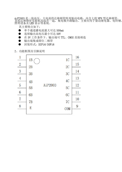
AiP2003是一块高压、大电流的达林顿管阵列驱动电路，内含七组NPN型达林顿管，各组达林顿管发射机均连在一起，集电极开路输出。

主要应用于驱动继电器、电铃锤、照明设备及LED显示等系统。

其主要特点如下：●单个通道灌电流最大可达500mA●连续输出高电压最小可达50V●在5V工作条件下，输出端可TTL、CMOS直接相连●输出端集成钳位二极管●封装形式：DIP16/SOP162、功能框图及引脚说明AiP2002是单片集成高耐压、大电流达林顿管阵列，电路内部包含五个独立的达林顿管驱动单路。

电路内部设计有续流二极管，可用于驱动继电器、步进电机等电感性负载。

单个达林顿管集电极可输出500mA电流。

将达林顿管并联可实现更高的输出电流能力。

该电路可广泛应用于继电器驱动、照明驱动、显示屏驱动(LED)、步进电机驱动和逻辑缓冲器。

AiP2002的每一路达林顿管串联一个2.7K的基极电阻，在5V的工作电压下可直接与TTL/CMOS电路连接，可直接处理原先需要标准逻辑缓冲器来处理的数据。

其主要特点如下：●500mA集电极输出电流（单路）●耐高压50V●输入兼容TTL/CMOS逻辑信号●广泛应用于继电器驱动；●封装形式：DIP14/SOP14产品型号封装形式印标识管装数盒装管盒装数箱装盒箱装数AiP2002 PA DIP14 AiP200225PCS/管40管/盒1000PCS/盒10盒/箱10000PCS/箱AiP2002 VA SOP14 AiP200250PCS/管200管/盒10000PCS/盒5盒/箱50000PCS/箱产品型号封装形式打印标识编带盘装数编带盒装数箱装数AiP2002 VA SOP14 AiP20022500PCS/盘5000PCS/盒40000PCS/箱引脚排列图AiP2001是一块高压、大电流的达林顿管阵列驱动电路，内含三组NPN型达林顿管，各组达林顿管发射极均连在一起，集电极开路输出。

主要应用于驱动继电器、电铃锤、照明设备及LED显示等系统。

Windows Server 2003印表机分享管理

Hardware Requirements for Configuring a Print Server
A print server running one of the operating systems in the Windows Server 2003 family
Sufficient RAM to process documents
When a user searches for printers:
1. Active Directory finds the subnet object that corresponds to the IP subnet in which the user’s computer is located 2. Active Directory uses the value in the Location attribute of the subnet object to search for printers with the same value 3. Active Directory displays a list of printers whose Location value matches the Location value of the subnet object
What Are Shared Printer Permissions?
Permission Print Allows the user to: Connect to a printer and send documents to the printer. Perform the tasks associated with the Print permission. The user also has complete administrative control of the printer. The user can pause and restart the printer, change spooler settings, share a printer, adjust printer permissions, and change printer properties. Pause, resume, restart, cancel, and rearrange the order of documents that all other users submit. The user cannot send documents to the printer or control the status of the printer.

Microsoft OneNote 2003

Microsoft OneNote 2003
佚名
【期刊名称】《个人电脑》
【年(卷),期】2003(9)11
【摘要】Microsoft的产品在首次推出时往往都不会非常出色，但是，该公司新推出的笔记记录程序Microsoft OneNote 2003却是我们见到过的最好的首发亮相的Microsoft应用，这个方便的应用提供了记录笔记的简单界面，能记录的内容包括格式化文本、要点、图形、Web页面的片断甚至手写内容。

OneNore能非常方便地输入信息而且最重要的是日后还可以查找信息。

【总页数】1页(P26)
【正文语种】中文
【中图分类】TP317.1
【相关文献】
1.OneNote 2003妙用三则 [J], 张迎新
2.办公原来如此轻松--OneNote 2003新鲜试用 [J], 武金刚
3.团结就是力量 OneNote 2003记录会议内容（一） [J], 王兰富
4.团结就是力量——用OneNote 2003记录会议内容（二） [J], 王兰富
5.What you Need to Know Microsoft Office OneNote 2003 [J], PaulThurrott;林颖华
因版权原因，仅展示原文概要，查看原文内容请购买。

SAE TECHNICAL PAPER SERIES 2003-01-1015 EVOP Design of Experiments

400 Commonwealth Drive, Warrendale, PA 15096-0001 U.S.A. Tel: (724) 776-4841 Fax: (724) 776-5760 Web: 2003-01-1015EVOP Design of ExperimentsDonald P . LynchVisteon Corporation2003 SAE World CongressDetroit, MichiganMarch 3-6, 20032003-01-1015EVOP Design of ExperimentsDonald P. LynchVisteon Corporation Copyright © 2003 SAE InternationalABSTRACTEvolutionary Operation (EVOP) experimental design using Sequential Simplex method is an effective and robust means for determining the ideal process parameter (factor) settings to achieve optimum output (response) results. EVOP is the methodology of using on-line experimental design. Small perturbations to the process are made within allowable control plan limits, to minimize any product quality issues while obtaining information for improvement on the process. It is often the case in high volume production where issues exist, however off-line experimentation is not an option due to production time, the threat of quality issues and costs. EVOP leverages production time to arrive at the optimum solution while continuing to process saleable product, thus substantially reducing the cost of the analysis. Sequential Simplex is a straightforward EVOP method which can be easily used in conjunction with prior traditional screening DOE or as a stand-alone method to rapidly optimize systems containing several continuous factors.INTRODUCTIONUnderstanding the application and limitations of the DOE process and each experimental design strategy is an integral part of reaching an experiment's objectives. The DOE process and the strategies, along with their application, are reviewed so that the desired level of understanding is obtained. Evolutionary Operation (EVOP) experimental design using the Sequential Simplex method is introduced, as part of an applied approach, as an effective and robust means for determining the ideal process parameter (factor) settings to achieve optimum output (response) results. Additionally, it is suggested that EVOP can serve in an alternative approach as an integrated total DOE tool for special cases. An understanding of how the Sequential Simplex method works is provided because it is a requirement for proper application and obtaining the desired results. The processes, strategies and methods provided in this paper inevitably cause a paradigm shift in the approach to applying DOE principles. OVERVIEW OF EXPERIMENTAL DESIGN STRATEGYDOE DEFINEDExperimental design, more commonly called design of experiments (DOE), is an important statistical tool in many continuous improvement efforts. DOE is a vehicle of scientific method, giving unambiguous results that can be used for inferring cause and effect. DOE is a systematic set of experiments that allows one to evaluate the impact, or effect, of one or more factors without concern about extraneous variables or subjective judgments. In this experiment the factors are purposefully perturbed with the intent of determining their effect on the output. The method starts with the statement of the experimental objective and ends with the reporting of results. The results from a DOE may often lead to further experimentation and ultimately to optimization. The objective of any DOE is to eliminate non-statistically significant factors while determining the factors important in predicting the desired output or response.Factors, as mentioned previously, are the variables under investigation that are set to a particular value (level) during the experiment. These variables may be quantitative or qualitative. The factor levels should be set with the specific purpose of understanding their impact on the response variables. The term factor has a number of synonyms, including but not limited to: parameter, input, controlled variable, independent variable, cause and X variable.Response variables, as mentioned previously, are the results from the experimental run. These variables are the output that is typically of concern to the experimenter. An understanding of the relationship between the response variables and the factors is the desired outcome of the entire DOE effort. Once the relationship is understood the response variable can usually be optimized by setting the factors to their optimal levels. The term response variable has a number of synonyms, including but not limited to; response, output, uncontrollable variable, dependent variable, effect, Y variable, result and outcome.DOE PROCESSThe DOE process consists of four primary phases: the objective / planning phase, the screening phase, the optimization phase and the confirmation phase.The objective / planning phase is often minimized by most practitioners despite being a vital component to achieving the desired results from the DOE effort. Time spent in the objective / planning phase will set the stage for success on all of the following phases. The purpose of the objective / planning phase is to clearly define the purpose and objectives of the experiment, obtain an understanding of all of the potential variables and devise a conscious strategy on how to address them in experimentation and perform measurement system and stability assessments. The purpose of the experiment should be consistent with a practical problem statement. In DOEs there are three potential objectives: maximize, minimize, hit a target and minimize variation.As previously suggested an important task in the objective / planning phase is to obtain an understanding of all of the potential variables that make up the process. These include input variables or factors, output variables or response as well as any signal variables that initiate the process. No variables should be omitted at this point, even if minimal impact on the analysis is anticipated. Once identified, it is important to classify all of the variables as controllable or uncontrollable and to define a conscious choice strategy for addressing each variable. This strategy will outline how to handle the variable throughout the analysis.Another step in the objective / planning phase is to perform the measurement system and stability assessments. The measurement system is analyzed to ensure that it is capable of detecting differences in the response. If the DOE objective is to minimize variation, the measurement system may have to be analyzed again as the variation is reduced. Prior to commencing the experiment, it is important to understand the state of control and stability of the process.The second phase of the DOE process is the screening phase. The goal of the screening phase is simply to identify the variables (factors) that have a significant effect on the response. A secondary goal is efficiency. The screening process should be accomplished as cost effectively and quickly as possible. During the screening phase the focus is not on the development of a mathematical model, but on understanding the few potentially significant variables that have an effect on the response.In order to accomplish the above goals, the screening phase involves selection of the ideal experimental design. This is a significant point in the efficiency of the experiment. It is a difficult task sometimes to strike a balance between the efficiency that is derived from the level of confounding and the clarity of the results. Screening design results often lead to further experimentation as the cause and effect relationship is progressively revealed. Some continuous improvement efforts will cease with the understanding that the screening phase provides. This is especially the case in less complex problems. While this approach may lead to significant improvements, and the optimization phase is not essential in every case, the results should always be confirmed.The third phase of the DOE process is the optimization phase. The purpose of the optimization phase is to carry the input from the screening phase and determine optimal factor level settings that generate the desired response. This can be accomplished by the development of a mathematical model or by means of using iterative approaches, such as EVOP. Both approaches have advantages and disadvantages. Development of a mathematical model requires the use of numeric methods and/or math programming applied to the model to arrive at the optimum results. While the model provides a significant amount of information about the process, the fit of the mathematical model is always a concern. An iterative approach is much more straightforward in application. The issues about model fit are not a concern. An iterative approach however does not provide the level of understanding of the process that a mathematical model provides. Using either approach in this phase translates the realization of the objective of the DOE. As stated previously, when an understanding of the statistically significant variables is all that is desired, this phase may be circumvented.The final phase in the DOE process is the confirmation phase. The purpose of the confirmation phase is to ensure that the results from the DOE analysis correlate with the actual process. This phase is critical to verify the effectiveness of the predictive power of the results and to ensure their reliability. This confirmation is typically performed by operating the process at the optimal factor level settings, suggested by the analysis and comparing the actual process response results with the predicted response from the analysis. Once the confirmation run has been completed the results from the DOE efforts can be used in the area of concern outlined in the study.In addition to performing a confirmation of the results after optimization, there may be benefits to confirm the results obtained at any early phase in the process. This is especially the case when the screening results are all that are desired or if a mathematical model is developed. Performing a confirmation at early stages in addition to after optimization, will help to minimize errors in the experimentation and save time that these errors create.TYPES OF DOE STRATEGIESThere are a number of DOE strategies that vary in complexity and nature. These strategies include one factor at a time (OFAT), full factorial, fractional factorial, response surface and EVOP. An understanding of the application and limitation of these strategies is critical for effective application of DOE methodology. The strategies can be classified as off-line or on-line.Off-line vs. On-line DOEOff-line or traditional DOE deals with running separate experimentation outside the normal process activity. This type of experimentation is performed off-line, because the experimental efforts typically produce product with responses that are not within the range of acceptability. This is caused from operating the process at factor levels outside of the allowable control plan limits. The product resulting from experimentation is for the intended purpose of analysis and frequently not saleable to a customer. Off-line DOE generally requires separate experimentation time and resources such as material and personnel required to operate the process. The primary benefits from off-line DOEs are the factor level settings applied are typically much wider than in an on-line approach. These wider factor level settings allow for a deeper understanding of the cause and effect relationship between factors and the response as well as a larger area of concern addressed by the analysis. This is especially important in cases when the optimal factor level settings fall outside the normal operating range. Applying an off-line DOE approach improves the potential for achieving breakthrough performance results by improving chance for identifying a global optimum condition.The primary issue with an off-line DOE approach is the need for additional resources increasing the cost required to run experimentation at separate times and with separate materials and personnel. Another potential issue with off-line DOE is the availability of the process for experimentation. If a process is fully utilized it may be difficult to find the necessary time to run the experimentation. This may lead to performing the experiment on premium time, further increasing the cost. It may even result in the inability to schedule the experiment at all. Additionally, many continuous processes (i.e. glass manufacturing, casting, mills) may not lend themselves to the short batch runs suggested in an off-line approach.On-line DOE is the opposite of off-line. In on-line DOEs the experimentation is typically run in conjunction with the normal process activity. The factors are perturbed in sufficiently small increments that product resulting from the experiment is typically within acceptable quality levels. Since most on-line DOEs are run with normal production with factor levels within control plan ranges, the product is often saleable.The primary benefit from on-line DOE is the cost savings associated with running saleable product over normal production time. The resources required for the experimentation are already available due to normal process activity. Additionally, due to resource availability and product quality, sample size is not of concern as in an off-line DOE. Since process is being operated in normal production time, the analysis can take advantage of very large sample sizes.The primary issue with an on-line DOE is the limited range of concern that results from the minimal perturbation of the factor levels. The factor level perturbations are limited to the specification ranges of acceptable product outlined in the control plan. This poses a concern only if the factor level settings producing the optimal response occur outside of the specification range.Interactions and ConfoundingSome other important concepts in dealing with different DOE strategies are interactions and confounding. Interactions are coupled effects where the response under consideration is dependent upon two or more factors. Many complex processes have interaction effects making it difficult to infer cause and effect without the use of experimental design methods. Typically, interaction effects involving more than two factors (three way interactions and higher) are assumed to not be statistically significant. However this assumption should be confirmed. Interactions need to be explicitly accounted for in off-line DOEs.The fact that higher order interaction effects are not typically statistically significant, allows them to be combined with effects from other factors that have a larger probability of being significant. This combining of effects is called confounding. Confounding significantly reduces the number of factor level combinations to be run, increasing the efficiency of the design. The increased efficiency reduces the amount of information provided from the analysis. When two factors are confounded it is impossible to determine which factor is responsible for the impact on the response. As previously stated, the higher order interaction factor is assumed to not be statistically significant signifying the other factor as the contributor to the effect. The clarity of the experiment is dependent on the level confounding. As previously suggested, a balance has to be struck between the efficiency improvements derived from the level of confounding and the clarity of the experiment. OFATGenerally, One Factor At a Time, commonly abbreviated OFAT, is not normally referred to as an experimentaldesign strategy due to its simple nature and limitations for use. However, OFAT is included as an experimental design strategy because it is intuitive, and if applied appropriately, can be used to assist in screening potentially significant factors and to resolve confounding. OFAT is the process of determining the impact of one factor on the response at a time. The response impact from the factor under consideration is perturbed while other factors are held constant. The process is repeated for each factor. This methodology can provide insight from a screening perspective to resolve confounding issues as well as to perform verification runs.The primary benefit of OFAT is intuitiveness and simplicity. It can be used off-line, although it is typically performed on-line if the factor level perturbations are within the specification ranges.The primary issue with OFAT is that it is less efficient than a factorial screening design, can provide incorrect conclusions in the face of strong interactions among factors and is less scientific then other DOE strategies. If an interaction is statistically significant and an OFAT strategy is applied, depending on what factor level is selected, different conclusions could be drawn. The issue of interactions and perceptions surrounding the scientific nature of OFAT are the reasons that it is not typically included as an experimental design strategy.Full FactorialFull factorial is an experimental design strategy where all factor level combinations are run. A response is observed at each of the factor level combinations to determine which factors have a statistically significant impact on the response. A full factorial experiment provides the most insight into the cause and effect relationship and in developing a mathematical model since there is no confounding present. All interaction effects are included in a full factorial experiment and it is run as a separate off-line experiment. A full factorial design is often used by entry-level practitioners of DOE because of the simplicity derived from the absence of confounding. A full factorial should not typical be performed in practice due to the large number of runs required by the multiple treatment combinations, leading to efficiency concerns. With some knowledge and a balance between the clarity of the experiment and level of confounding, the same information can be drawn from a fractional factorial experiment.Fractional FactorialLike the full factorial the fractional factorial experimental design strategy is used for screening, but not to develop a mathematical model. The goal of the fractional factorial screening effort is to conclude which factors are statistically significant and should be included in further experimentation. As previously stated, the goal of the fractional factorial is not to develop a mathematical model nor is it to determine the optimal factor level settings. Also, as previously stated some continuous improvement efforts will stop with the identification of the statistically significant factors.Fewer runs are required for the fractional factorial experiment as not all factor level combinations are considered. Fractional factor experiments take advantage of confounding, allowing for the increased efficiency of the design. However, information concerning higher order interaction effects are not available. An understanding of the assumptions and the confounding pattern is required to draw the conclusions regarding the factors that are significant. Similar to full factorial experiments, fractional factorial experiments are run as separate off-line experiments. Fractional factorial experimental designs are the preferred choice for initial screening designs.Response Surface MethodologyResponse Surface Methodology is used for more complex analysis involving non-linearity and for optimization. A response surface is a topographical representation of the response over a region of concern, outlined by the factor level ranges. Response Surface Methodology is typically implemented as a sequential experiment, starting with larger regions and progressively moving to smaller regions as the optimum response area is identified. A mathematical model may be developed or results from a response surface analysis may serve as input to an alternative optimization strategy like EVOP.EVOPEvolutionary Operation (EVOP) is an evolutionary, iterative path of steepest ascent method for determining the optimum factor level settings. EVOP is not typically considered an experimental design strategy as it is used for optimization. However it can also be used as a DOE strategy as outlined below. EVOP is a very effective, simple and cost effective tool that does not require the development of a mathematical model. When used for optimization the information gained from prior DOE strategies serve as input to EVOP.EVOP is considered an off-line DOE strategy and has allof the corresponding advantages associated with this strategy. One of the major advantages of EVOP is that there are no confounding issues and interactions are handled implicitly. This is a substantial advantage when being applied by most practitioners who are not expertsin DOE methodologies. For this reason it is often performed in manufacturing environments using small changes in factor level settings and large sample sizes, while being non-disruptive to the manufacturing process, thus producing saleable product. Outside of manufacturing, EVOP is also a valuable approach as an alternative to Response Surface Methodology. Listed inTable 1 is a summary comparison of EVOP Sequential Simplex to Response Surface Methodology (RSM). EVOP Sequential Simplex RSMNo underlying mathematical model Based on a mathematical modelIf “k” = # factors, need (k+1) points to start, with 1 additional point per step If “k” = # factors, need 3k points to start, and 3k points for each stepSeeks optimum “point”Seeks optimum settings,with some information onsurrounding regionsInformation on “path” to optimum Information collected for “regions” of operationBetter suited for ongoing manufacturing process improvement Better suited for design optimization, or brand new manufacturing processTable 1. EVOP to RSM ComparisonsEXPERIMENTAL DESIGN APPROACHESThe basis of most academic experimental design approaches is a mathematical model. The progressive academic approach consists of the following steps to accomplish the experimental objective:Academic Approach1. Planning Phase2. Fractional Factorial - the use of a fractional factorialdesign for screening of potential statistically significant factors3. Full Factorial – the use of a full factorial design fordevelopment of a linear mathematical model4. Response Surface Design – if improved accuracy isdesired, the use of a Response Surface Design fordevelopment of a non-linear mathematical model5. Mathematical Optimization – the use ofmathematical optimization on the model developedin prior steps to establish the optimal factor levelsettingsWhile the academic approach has merit in many projects, it is limited by the assumption of the mathematical model. Any gaps in performance of the mathematical model mirroring the actual process results in inaccuracy in optimal settings. A more robust approach is an applied approach in which a mathematical model does not limit the results of the analysis. The progressive applied approach consists of the following steps to accomplish the experimental objective:Applied Approach1. Planning Phase2. Fractional Factorial - the use of a fractional factorialdesign for screening of potential statistically significant factors3. Response Surface Design – not for the developmentof a mathematical model but the establishment of the starting point, if a better starting point is desired 4. EVOP Optimization – the use of EVOP optimization,with input from the prior analysis, to determine the optimal factor level settingsThe applied approach offers advantages over the academic approach in its implementation simplicity, efficiency and cost effectiveness, and accuracy due to the absence of the mathematical model assumption. However, the development of the mathematical model does provide one advantage in the academic approach in that the model provides more information about the process. The mathematical model can be used to predict specific responses at operating ranges other than the optimal. This is particularly important when analyzing "what-if" scenarios.There is a third approach that is an option when on-line DOE is not available. The academic and applied approaches do not lend themselves to analysis where off-line separate experimentation is not an option, as in the case where processes are scheduled without interruption or for continuous processes. In these special cases there is a third approach, referred to as the alternative approach that consists of the following steps to accomplish the experimental objective: Alternative Approach1. Planning Phase2. EVOP Optimization - the use of EVOP optimization,with no input from prior analysis, to determine the optimal factor level settingsWhile there is a definite application, this alternative approach has some serious limitations. The only other option in these special cases where only on-line DOE is acceptable is an OFAT methodology. One limitation in the alternative approach is the fact that the true optimization point may fall outside of the specification range used in the EVOP analysis. An additional concern is the cost of carrying the non-statistically significant factors during the experiment then controlling them in production. Carrying the additional non-statistically significant factors increases the cost of the EVOPHow Does is it Work?2 analysis through increased samples size and alsoincreases the complexity of the analysis, reducing thechance of arriving at the correct optimal. Regarding the production cost in the prior approaches, once a factor is determined to not be statistically significant, it is typically set to the level that achieves the lowest cost performance. A final concern is that if some potentially statistically significant variables are not included in the analysis, it would be very difficult to recognize and the derived results may be incorrect. The simplest case of the Sequential Simplex method is the fixed step size. In this case the size of the steps taken to arrive at the optimal condition do not change. The procedure for the fixed step size for the simplex is outlined below and displayed graphically for the specific case when k=2, in Figure 1.1. Choose initial simplex2. Experiment at each setting defined by the vertices ofthe simplexThe advantages of the alternative approach are that it isvery simple and straightforward to perform. It also eliminates the possibility of making an error in any prior factorial experimentation. These errors are primarily centered on the determination of statistically significant variables in the face of confounding and interactions. As stated previously, EVOP handles interactions implicitly. Finally, for special cases, it is the only alternative DOE strategy other than OFAT. 3. Rank the vertices as best, next best and worstbased on the response4. Calculate the "reflection" of the worst point andexperiment at the reflection5. Go back to step 3 and repeat until optimum isreachedIn summary EVOP can be used in two ways. As outlined in the applied approach, EVOP can be used as an optimization tool. In this application factorial designs and potentially even RSM can be used as an input, with the optimal factor level settings corresponding to the optimum response as the output. As outlined in the alternative approach, EVOP can be used as an integrated total DOE tool. In this application the important process factors are the input, and the optimal factor level settings corresponding to the optimum response as the output.EVOP PRINCIPLESSEQUENTIAL SIMPLEX METHODThe most popular EVOP method is the Sequential Simplex method. A simplex is defined as; an element or figure contained within Euclidean space of a specified number of dimensions and having one more boundary point than the number of dimensions.1 Restated, the simplex is the simplest geometric shape required to define an expression. The Sequential Simplex method is an evolutionary, geometrical iterative path of steepest ascent method for determining the optimum factor level settings. In setting up a simplex, the initial simplex shape requires k+1 points (k being the number of experimental factors). This is substantially less than the factorial approach that has at least 2k and possibly 3k or 4k points to start. In addition, only one new trial is required to move to a new area in the space defined by the factors. A factorial design requires at least 2k-1 trials. As mentioned in EVOP, another major advantage of the Sequential Simplex method, is that a mathematical model does not have to be assumed. All decisions are based on ranking of vertices of the simplex.2VariableX2Figure 1. Fixed Step Size SimplexThe fixed step size is the simplest form of the simplex, but the simplicity causes some inadequacies. The primary issue with the fixed step size is the criticality of the size of the step. If a large step size is selected, the optimum will never be obtained because of resolution issues. If a small step size is selected, an excessive number of points is required to reach the optimum. A solution to address the above issues is a variable step size simplex.2The variable size simplex follows the same procedure as outlined above, except in place of only an option of a reflection on the worst point, the variable size simplex offers three other alternatives: contract worst (CW), contract reflection (CR) and extension (E). The。

A comprehensive review of the development of zero waste management_ lessons learned and guidelines

Journal of Cleaner Production 91 (2015) 12e25
Contents lists available at ScienceDirect
Journal of Cleaner Production
journal homepage: /locate/jclepro
Review
A comprehensive review of the development of zero waste management: lessons learned and guidelines
Atiq Uz Zaman
Zero Waste SA Research Centre for Sustainable Design and Behaviour (sdþb), School of Art, Architecture and Design, University of South Australia, G.P.O. Box 2471, SA 5001, Australia
a r t i c l e i n f o
Article history: Received 29 August 2014 Received in revised form 17 October 2014 Accepted 4 December 2014 Available online 12 December 2014 Keywords: Waste management Zero waste concept Zero waste study Zero waste strategy
E-mail address: atiq.zaman@.au. /10.1016/j.jclepro.2014.12.013 0959-6526/© 2014 Elsevier Ltd. All rights reserved.

2003芯片

2003 THRU 2024x = digit to identify specific device. Characteristic shown applies to family of devices with remaining digits as shown. See matrix on next page.Data Sheet 29304FIdeally suited for interfacing between low-level logic circuitry and multiple peripheral power loads, the Series ULN20xxA/L high-voltage,high-current Darlington arrays feature continuous load current ratings to 500 mA for each of the seven drivers. At an appropriate duty cycle depending on ambient temperature and number of drivers turned ON simultaneously, typical power loads totaling over 230 W (350 mA x 7,95 V) can be controlled. Typical loads include relays, solenoids,stepping motors, magnetic print hammers, multiplexed LED andincandescent displays, and heaters. All devices feature open-collector outputs with integral clamp diodes.The ULN2003A/L and ULN2023A/L have series input resistors selected for operation directly with 5 V TTL or CMOS. These devices will handle numerous interface needs — particularly those beyond the capabilities of standard logic buffers.The ULN2004A/L and ULN2024A/L have series input resistors for operation directly from 6 to 15 V CMOS or PMOS logic outputs.The ULN2003A/L and ULN2004A/L are the standard Darlington arrays. The outputs are capable of sinking 500 mA and will withstand at least 50 V in the OFF state. Outputs may be paralleled for higher load current capability. The ULN2023A/L and ULN2024A/L will withstand 95 V in the OFF state.These Darlington arrays are furnished in 16-pin dual in-line plastic packages (suffix “A”) and 16-lead surface-mountable SOICs (suffix “L”). All devices are pinned with outputs opposite inputs to facilitate ease of circuit board layout. All devices are rated for operation over the temperature range of -20°C to +85°C. Most (see matrix, next page) are also available for operation to -40°C; to order, change the prefix from “ULN” to “ULQ”.FEATURESI TTL, DTL, PMOS, or CMOS-Compatible Inputs I Output Current to 500 mA I Output Voltage to 95 V I Transient-Protected OutputsI Dual In-Line Plastic Package or Small-Outline IC PackageHIGH-VOLTAGE, HIGH-CURRENTDARLINGTON ARRAYSDwg. No. A-959416151413126117108912345Note that the ULN20xxA series (dual in-line package) and ULN20xxL series (small-outline IC package) are electrically identical and share a common terminal number assignment.ABSOLUTE MAXIMUM RATINGSOutput Voltage, V CE(ULN200xA and ULN200xL)........ 50 V (ULN202xA and ULN202xL)........ 95 V Input Voltage, V IN ................................ 30 V Continuous Output Current,I C ................................................. 500 mA Continuous Input Current, I IN ........... 25 mA Power Dissipation, P D(one Darlington pair)..................... 1.0 W (total package)....................... See Graph Operating Temperature Range,T A .................................. -20°C to +85°C Storage Temperature Range,T S ................................. -55°C to +150°C查询2003供应商2003 THRU 2024HIGH-VOLTAGE,HIGH-CURRENTDARLINGTON ARRAYS115 Northeast Cutoff, Box 15036Worcester, Massachusetts 01615-0036 (508) 853-5000V CE(MAX)50 V95 VI C(MAX)500 mA500 mALogic Part Number5VULN2003A*ULN2023A*TTL, CMOS ULN2003L*ULN2023L 6-15 V ULN2004A*ULN2024A CMOS, PMOSULN2004L*ULN2024L*Also available for operation between -40°C and +85°C. To order, change prefix from “ULN” to “ULQ”.Dwg. No. A-9651COM7.2K 3K2.7KX = Digit to identify specific device. Specification shown applies to family of devices with remaining digits as shown. See matrix above.Copyright © 1974, 1998 Allegro MicroSystems, Inc.Dwg. No. A-9898AULN20x4A/L (Each Driver)COM7.2K 3K10.5K50751001251502.50.5A L L O W AB L E P AC K A G E P O W E RD I S S I P A T I O N I N W A T T SAMBIENT TEMPERATURE IN °C2.01.51.025SUFFIX 'L', R = 90°C/W θJADwg. GP-006ASUFFIX 'A', R = 60°C/W θJAULN20x3A/L (Each Driver)DEVICE PART NUMBER DESIGNATIONPARTIAL SCHEMATICS2003 THRU 2024HIGH-VOLTAGE,HIGH-CURRENT DARLINGTON ARRAYSTest Applicable Limits Characteristic Symbol Fig.DevicesTest Conditions Min.Typ.Max.Units Output Leakage CurrentI CEX1AA ll V CE = 50 V, T A = 25°C—< 150µA V CE = 50 V, T A = 70°C—< 1100µA 1BULN2004A/LV CE = 50 V, T A = 70°C, V IN = 1.0 V—< 5500µA Collector-Emitter V CE(SAT)2A llI C = 100 mA, I B = 250 µA—0.9 1.1V Saturation Voltagel C = 200 mA, I B = 350 µA— 1.1 1.3V I C = 350 mA, I B = 500 µA—1.3 1.6V Input CurrentI IN(ON)3ULN2003A/L V IN = 3.85 V —0.93 1.35mA ULN2004A/LV IN = 5.0 V —0.350.5mA V IN = 12 V— 1.0 1.45mA I IN(OFF)4A ll l C = 500 µA, T A = 70°C5065—µA Input VoltageV IN(ON)5ULN2003A/LV CE = 2.0 V, l C = 200 mA—— 2.4V V CE = 2.0 V, I C = 250 mA—— 2.7V V CE = 2.0 V, l C = 300 mA—— 3.0V ULN2004A/LV CE = 2.0 V, l C = 125 mA—— 5.0V V CE = 2.0 V, l C = 200 mA—— 6.0V V CE = 2.0 V, I C = 275 mA——7.0V V CE = 2.0 V, l C = 350 mA——8.0V Input Capacitance C IN —A ll —1525pF Turn-On Delay t PLH 8All 0.5 E IN to 0.5 E OUT —0.25 1.0µs Turn-Off Delay t PHL 8All0.5 E IN to 0.5 E OUT —0.25 1.0µs Clamp DiodeI R 6A llV R = 50 V, T A = 25°C ——50µA Leakage Current V R = 50 V, T A = 70°C——100µA Clamp Diode V F7A llI F = 350 mA—1.72.0VForward VoltageComplete part number includes suffix to identify package style: A = DIP, L = SOIC.Types ULN2003A, ULN2003L, ULN2004A, and ULN2004LELECTRICAL CHARACTERISTICS at +25°C (unless otherwise noted).2003 THRU 2024HIGH-VOLTAGE,HIGH-CURRENTDARLINGTON ARRAYS115 Northeast Cutoff, Box 15036Worcester, Massachusetts 01615-0036 (508) 853-5000Test Applicable Limits Characteristic Symbol Fig.DevicesTest ConditionsMin.Typ.Max.Units Output Leakage CurrentI CEX1AA ll V CE = 95 V, T A = 25°C—< 150µA V CE = 95 V, T A = 70°C—< 1100µA 1BULN2024A/LV CE = 95 V, T A = 70°C, V IN = 1.0 V—< 5500µA Collector-EmitterV CE(SAT)2A llI C = 100 mA, I B = 250 µA—0.9 1.1V Saturation Voltagel C = 200 mA, I B = 350 µA— 1.1 1.3V I C = 350 mA, I B = 500 µA—1.3 1.6V Input CurrentI IN(ON)3ULN2023A/L V IN = 3.85 V —0.93 1.35mA ULN2024A/LV IN = 5.0 V —0.350.5mA V IN = 12 V— 1.0 1.45mA I IN(OFF)4A ll l C = 500 µA, T A = 70°C5065—µA Input VoltageV IN(ON)5ULN2023A/LV CE = 2.0 V, l C = 200 mA—— 2.4V V CE = 2.0 V, I C = 250 mA—— 2.7V V CE = 2.0 V, l C = 300 mA—— 3.0V ULN2024A/LV CE = 2.0 V, l C = 125 mA—— 5.0V V CE = 2.0 V, l C = 200 mA—— 6.0V V CE = 2.0 V, I C = 275 mA——7.0V V CE = 2.0 V, l C = 350 mA——8.0V Input Capacitance C IN —A ll —1525pF Turn-On Delay t PLH 8All 0.5 E IN to 0.5 E OUT —0.25 1.0µs Turn-Off Delay t PHL 8All0.5 E IN to 0.5 E OUT —0.25 1.0µs Clamp Diode I R 6A llV R = 95 V, T A = 25°C ——50µA Leakage Current V R = 95 V, T A = 70°C——100µA Clamp Diode V F7A llI F = 350 mA—1.72.0VForward VoltageComplete part number includes suffix to identify package style: A = DIP, L = SOIC.Types ULN2023A, ULN2023L, ULN2024A, and ULN2024LELECTRICAL CHARACTERISTICS at +25°C (unless otherwise noted).2003 THRU 2024HIGH-VOLTAGE,HIGH-CURRENT DARLINGTON ARRAYSOPENOPENV CEI CEXµAV INOPENV CEI CEXµAI BOPENh FE =V CE VICI BI CV INOPENmAOPENI INOPENV CEI CµAI INµAVOPENV CEVV INI COPENV RI RµAI FOPENV FV 50%50%50%50%t pHLt pHLOUTPUTINPUTV INPULSE GENERATOR PRR = 10KHz DC = 50%INPUT 93 Ω50 pFOUT 30 Ω100 Ω+50 VDwg. No. A-9732A Dwg. No. A-9733ADwg. No. A-9734AFIGURE 6FIGURE 7FIGURE 8Dwg. No. A-9735ADwg. No. A-9736AV inULN20X3* 3.5 V ULN20X4*12 VTEST FIGURESFIGURE 1AFIGURE 1BFIGURE 2FIGURE 3FIGURE 4FIGURE 5*Complete part number includes a final letter to indicate package.X = Digit to identify specific device. Specification shown applies to family of devices with remaining digits as shown.Dwg. No. A-9731ADwg. No. A-9730ADwg. No. A-9729A115 Northeast Cutoff, Box 15036Worcester, Massachusetts 01615-0036 (508) 853-5000Dwg. GP-067COLLECTOR-EMITTER SATURATION VOLTAGE Dwg. GP-068INPUT CURRENT IN µA2003 THRU 2024HIGH-VOLTAGE,HIGH-CURRENT DARLINGTON ARRAYSTYPICAL APPLICATIONSINPUT CURRENTAS A FUNCTION OF INPUT VOLTAGETypes ULN2004A, ULN2004L, ULN2024A, andULN2024L16151413126117108912345Dwg. No. A-9653A+V+V CCTTLOUTPUT16151413126117108912345Dwg. No. A-10,175+V+V CCTTL OUTPUTR PTypes ULN2003A, ULN2003L, ULN2023A, andULN2023L3.0Dwg. GP-0695.06.0INPUT VOLTAGE2.02.52.0I N P U T C U R R E N T I N m A — II N1.0MA X I M U M 0.51.54.0AREA OF NORMAL OPERATION WITH STANDARD OR SCHOTTKY TTLT Y P I C A L6Dwg. GP-069-11012INPUT VOLTAGE52.0I N P U T C U R R E N T I N m A — I I N1.0M AX I M U M0.51.58T Y P IC A L 79112003 THRU 2024HIGH-VOLTAGE,HIGH-CURRENTDARLINGTON ARRAYS115 Northeast Cutoff, Box 15036Worcester, Massachusetts 01615-0036 (508) 853-5000PACKAGE DESIGNATOR “A”Dimensions in Inches (controlling dimensions)Dimension in Millimeters (for reference only)NOTES:1.Leads 1, 8, 9, and 16 may be half leads at vendor’s option.2.Lead thickness is measured at seating plane or below.3.Lead spacing tolerance is non-cumulative.4.Exact body and lead configuration at vendor’s option within limits shown.Dwg. MA-001-16A mm16189Dwg. MA-001-16A in161892003 THRU 2024HIGH-VOLTAGE,HIGH-CURRENT DARLINGTON ARRAYSPACKAGE DESIGNATOR “L”Dimensions in Inches (for reference only)Dimension in Millimeters (controlling dimensions)NOTES:1.Lead spacing tolerance is non-cumulative.2.Exact body and lead configuration at vendor’s option within limits shown.Dwg. MA-007-16A mm169Dwg. MA-007-16 in1692003 THRU 2024HIGH-VOLTAGE,HIGH-CURRENTDARLINGTON ARRAYS115 Northeast Cutoff, Box 15036Worcester, Massachusetts 01615-0036 (508) 853-5000The products described here are manufactured under one or more U.S. patents or U.S. patents pending.Allegro MicroSystems, Inc. reserves the right to make, from time to time, such departures from the detail specifications as may be required to permit improvements in the performance, reliability, ormanufacturability of its products. Before placing an order, the user is cautioned to verify that the information being relied upon is current.Allegro products are not authorized for use as critical components in life-support devices or systems without express written approval.The information included herein is believed to be accurate and reliable. However, Allegro MicroSystems, Inc. assumes no responsi-bility for its use; nor for any infringement of patents or other rights of third parties which may result from its use.。

1、下载文档前请自行甄别文档内容的完整性，平台不提供额外的编辑、内容补充、找答案等附加服务。
2、"仅部分预览"的文档,不可在线预览部分如存在完整性等问题,可反馈申请退款(可完整预览的文档不适用该条件!)。
3、如文档侵犯您的权益，请联系客服反馈,我们会尽快为您处理(人工客服工作时间：9:00-18:30)。

UNIVERSITY OF SOUTHAMPTONSEMESTER1EXAMINA TION2008/09ECON2003Microeconomics TheoryDuration:120minsAnswer ALL questions from section A,and ONE question from Section BUniversity approved calculators may be usedA foreign language translation dictionary is permittedprovided it contains no notes,additions or annotations.Electronic dictionaries are not permitted.Copyright2009c University of Southampton Number of pages5Section A1(15points)Mario has16hours per day to allocate between leisure and working at a wage of£5per hour.Mario’s utility function is u(x;l)=x (16 l)where x is the amount of consumption good he consumes and l is his supply of labour.Each day Mario also receives a…xed income of£10(e.g.from some savings in his bank).(a)Draw Mario’s budget constraint between leisure hours on the hor-izontal axis and consumption on the vertical axis.(Assume the price of consumption goods is£1/unit.)(b)Determine the optimal demand for the consumption good and the optimal supply of labour.2(15points)Consider a…rm using a Cobb-Douglas technology given by q=f(l;k)=l1=2k1=2;and facing factor prices w=1and r=4 for labour and capital,respectively.Assume that in the short-run,the quantity of capital is…xed and equal to225.(a)W rite the cost of the…rm as a function of the output,C(q),distin-guishing…xed costs and variable costs.(b)What are the average cost,average variable cost and marginal cost? Assume that in the long-run,both of the inputs can be adjusted. (c)W rite the…rm’s cost minimization problem and determine the…rst order conditions.(d)What are the factor demand functions(i.e.l(w;r;q)and k(w;r;q)) and the cost function c(w;r;q)of the…rm?3(15points)A patent gives Sony a legal monopoly to produce a robot dog called Aibo.Sony wants to sell this robot in the USA and in the EU.The American inverse demand function is p US=4500 Q US,and the EU inverse demand function is p EU=3500 12Q EU(assumethat both prices are measured in dollars).Sony’s marginal cost of producing Aibo is$500in both areas.(a)If Sony can prevent resales,what prices will it charge to the US and EU consumers?(b)Using the results in part(a),determine the elasticity of the demand in the two areas.(c)Show how the ratio of the prices determined in part(a)depends on the elasticities of demand determined in part(b).4(15points)Consider a little exchange economy with only two agents: Robinson Crusoe and Friday.In this economy there are only two products:bananas(b)and…shes(f).Robinson preferences are such that he always wants the same quantity of…sh and bananas.That is, eating one extra…sh without having one extra banana does not give him any utility.Friday instead likes…sh better than bananas and he is always happy to exchange one…sh for two bananas.Assume that today Robinson’s endowment is5bananas and2…shes,while Friday’s endowment is5bananas and5…shes.(a)Draw the Edgeworth box representing this economy(use bananas on the horizontal axes).(b)Draw the indi¤erence curves of Robinson(bottom left of the box) and Friday(top right of the box).(c)Draw all the Pareto e¢cient allocations and specify what alloca-tions are in the CORE(i.e.all Pareto optimal allocations that are Pareto superior to the initial allocation).5(15points)Mario has a concave utility function of U(W)=W0:5:His only asset is shares in an Internet company.T omorrow he will learn the stock’s value.He believes that this will be£144with probability 2/3and£225with probability1/3.(a)What is his expected wealth?(b)What is his expected utility?(c)What risk premium would he pay to avoid bearing this risk?TURN OVERSection B6(25points)Two…rms,X and Y,have access to…ve di¤erent produc-tion processes,each one of which has a di¤erent cost and gives o¤a di¤erent amount of pollution.The daily cost of the processes and the corresponding number of tons of smoke are listed in the table below.Pr ocess (smoke)A(4tons)B(3tons)C(2tons)D(1ton)E(0tons)Cost to…rm X10015030010002000Cost to…rm Y5070100140200 Assume that pollution is unregulated.(a)What process would the two…rms choose?How many tons of pol-lution per day would the…rms emit?Assume now that the city council wants to cut the smoke emissions de-termined in question(a)by half.T o accomplish this,they are considering two options.The…rst is to require each…rm to curtail its emissions by half.The alternative is to set a tax of T on each ton of smoke emitted each day.(b)How large would T have to be in order to cut emissions by half? [Hint:The tax is aimed at reducing total emissions by half,not neces-sarily the emissions of each…rm](c)And how would the total costs to society compare under the two alternatives?[Hint:The tax paid by the two…rms are revenues for the government, so their net e¤ect on social costs is zero]7(25points)Consider a simple economy composed of two agents,Robin-son(R)and Friday(F),and3goods,bananas(x b),…shes(x f)and water(x w).Assume that in this economy bananas are the numeraire (so their price is p b=1).Because of large rain falls,Robinson and Friday can drink any quantity of water they want for free(i.e.p w=0).Robinson has an initial endowment of10bananas and10…shes.Fri-day’s endowment is given by20bananas and10…shes.Assume thatRobinson and Friday has the same preferences,represented by the util-ity function:u R(x b;x f;x w)=u F(x b;x f;x w)=ln x b+ln x f+x w 12x2w.(a)W rite the maximization problem for the two agents.(b)Impose the…rst order conditions and…nd the demand functions of each agent.(c)Find the equilibrium prices and allocationsEND OF PAPER。