Coherence Cube相干体分析技术
地震属性体处理

地震属性体处理1、分频处理属性分频处理属性可将地震振幅和属性数据转换成更为清晰的地下地质图像,识别薄层或能量衰减区。
将各地震道分解成不同的频带成分,有助于突出复杂的断裂体系以及储层的分布特征。
分频处理的技术主要是通过“Gabor-Morlet” 子波对复数地震道进行谱分解,类似于小波变换。
用来帮助地质家和解释人员进行如下的勘探研究工作:(1)薄层检测以及薄层厚度估计;(2)衰减分析——直接进行油气检测(3)提高地震分辨率该方法通过连续的时频分析来描述时间--频率的瞬时信号能量密度。
与以往常规的谱分解使用离散傅立叶变换不同,该方法使用Gabor-Morley 子波来提高时间-频率的分辨率。
提供了两种计算瞬时能量的方法:等空间中心频率和倍频程频率。
输出结果可以分解成多种属性体:时间-频率体、时间切片,然后进行分析。
2、地震属性分析地震属性分析使我们获得更多极有价值的多方位信息,从而使油藏的描述更准确、更细致。
帕拉代姆地震属性库包括丰富的地震属性,如振福包络、瞬时频率、吸收系数以及相对波阻抗等20多种复地震道(Hilbert )属性、多道几何属性,谱分解属性和用户自定义属性见图。
这些地震属性可分别表征地震影像的不同特征,从而使解释人员以少量的工作即可获得大量的地质信息,其中多地震道几何属性包括倾角体、方位角体、非连续性和照明体。
这些属性旨在强化地震影像的非连续性特征,因此对识别地质体的构造特征(如断层)、地层边界、河道和地质体的几何样式十分有效。
在这些属性体提取的基础上,利用PCA 主组分分析技术进行属性优化分析,同时也可借助多属性体交会VXPLOT 识别异常体。
通过多属性体交汇、神经网络测井参数反演、多属性体的波形分类以及变时窗/等时窗的地震相划分等综合技术,并借助多属性体立体可视化浏览技术实现对地下构造、地层和储层岩性的综合解释。
常用提取的地震属性有信号包络、瞬时频率、瞬时相位、相对波阻抗、分频处理等。
地震数据相干体分析技术
地震数据相干体分析技术地震数据的相干体分析技术是一种利用地震数据中的相干性信息,来研究地震活动规律和地震源特征的方法。
相干体是指在一定时间段内,地震波传播路径上的地震信号的相位和振幅相对稳定,具有较高的相干度。
相干度是衡量两个地震信号之间相干性强弱的指标,可用于分析地震波的传播特征和地下介质的结构。
相干体分析技术主要包括相干度计算方法、相干体提取方法和相干体分析方法三个方面。
首先,相干度计算方法是相干体分析的基础。
常用的相干度计算方法有互相关法、谱相关法和小波变换法等。
互相关法通过计算两个信号的时间序列之间的相关系数,得到相干度值。
谱相关法是将信号在频域上进行相关计算,利用信号的频谱特征来计算相干度。
小波变换法是利用小波变换将信号分解成不同尺度和频率的小波系数,然后计算小波系数之间的相干度。
其次,相干体提取方法是从地震数据中提取相干体的过程。
常用的相干体提取方法有滑动窗口法、相干度阈值法和小波变换法等。
滑动窗口法将地震数据分成多个时间窗口,然后计算每个窗口内信号之间的相干度,得到相干度时间变化曲线,从中提取出相干度较高的时间段作为相干体。
相干度阈值法是根据相干度的统计特性设定一个相干度阈值,只有大于该阈值的相干度才被认为是相干体。
小波变换法将地震数据进行小波变换,然后计算小波系数之间的相干度,从中提取出相干度较高的小波系数作为相干体。
最后,相干体分析方法是利用提取到的相干体来研究地震活动规律和地震源特征。
常用的相干体分析方法有相干体叠加法、相干体分析法和相干体变化法等。
相干体叠加法是将相干度较高的地震信号进行叠加,放大地震信号的相干体特征。
相干体分析法是对提取到的相干体进行频谱分析、尺度分析和相位分析,从中获取地下介质的结构信息。
相干体变化法是对相干体的时间变化进行分析,研究地震源的演化特征和地震活动的周期性规律。
综上所述,相干体分析技术是一种重要的地震数据处理方法,可以用于地震波传播特征分析、地下介质结构研究和地震源特征分析等方面。
三维精细构造解释的方法流程和关键技术_刘丽峰
第21卷第3期地球物理学进展Vol.21 No.3三维精细构造解释的方法流程和关键技术刘丽峰, 杨怀义, 蒋多元, 董宁, 王相文(中国石油化工股份有限公司石油勘探开发研究院,北京100083)摘要详细论述了三维精细构造解释的方法和流程.对层位标定、层位解释、断裂、速度解释及成图每个步骤的方法给以具体论述,重点分析了三维精细构造解释使用的关键技术如可视化技术、相干体技术、变速解释技术和真三维解释技术.本文可为从事三维精细构造解释的人员提供借鉴.关键词三维精细构造解释,相干体,变速解释,真三维解释,虚拟现实技术中图分类号P631 文献标识码 A 文章编号1004-2903(2006)03-0864-08PrimaryExplorationof3-DFineStructureInterpretationLIUL-ifeng, YANGHua-iyi, JIANGDuo-yuan, DONGNing, WangXiang-wen(Exploration&ProductionResearchInstitute.SINOPEC,Beijing100083,China)Abstract Thisarticlesystemicallysummarizesthemethodandflowof3-Dfinestructureinterpretatio nanddescibes,everystepsuchashorizondemarcate、horizoninterpretation、faulting、velocityinterpretationandcartography.Espe-ciallyltexplainsthekeytechnology-visua lizingtechnology、coherencecubetechnology、velocity-variedinterpretationtechnology.Thisarticlecanbeusedasthereferencetothen oviceof3-Dfinestructureinterpretation.Keywords3-Dfinestructureinterpretation,coherencecube,velocity-variedinterpretation,true3 -DinterpretationVR0 引言随着三维地震勘探技术的发展,构造解释技术在近年来已有较大的发展.传统的三维解释方法是把三维地震资料当作加密的二维地震资料进行解释,存在信息利用率低,工作效率低,成果质量不高等问题,解释人员需要在层位解释和断层识别、组合上花费大量时间和精力.随着地震资料属性处理和人机联作解释方法的不断发展和成熟,打破常规的三维资料二维解释,充分利用三维数据信息,获得更精细的构造形态,高效、高精度的三维精细构造解释已经切实可行.三维可视化(VoxelGeo)技术[2]的不断发展,更是推动了三维解释技术,出现了真(全)三维地震解释技术.近年来,虚拟现实技术(VR)应用于三维地震资料的可视化解释,使地震资料解释更为自动化、智能化[3].目前,三维精细构造解释的支[1]持软件是Landmark地震解释软件和虚拟现实技术,Paradigm地震解释软件及可视化技术.1 三维精细构造解释三维精细构造解释的步骤是层位标定,层位、断层解释,速度解释和构造成图.1.1 层位标定构造解释的第一步是层位标定,首先分析比较分层数据的各层位划分情况,使分层数据准确一致;之后对声波测井曲线进行编辑,剔除畸变.并结合自然电位、自然伽玛、电阻率、密度等曲线提取井旁道地震子波制作单井合成记录;制作完单井的合成记录之后,再制作联井合成地震记录.结合VSP叠加地震剖面,进行粗框架地震剖面追踪对比,检查各反射波闭合情况,当存在不闭合时,依据钻井分层数据调整少数不闭合井的合成记录,并根据声波速度、地收稿日期 2006-02-10; 修回日期 2006-05-20.基金项目中石化东北分公司《松辽盆地南部长岭凹陷所图探区滚动勘探开发一体化研究》项目资助.作者简介刘丽峰,女,1974年生,河南遂平人,2003年于中国科学院地质与地球物理研究所获博士学位,现于中石化石油勘探开发研究院工作,主要从事综合地质、地球物理及构造解释方面的研究工作.。
相干体技术的基本原理
孙夕平相干算法论述相干体技术用于检测地震波同相轴的不连续性。
其基本原理是在偏移后的三维数据体中,对每一道每一样点求得与周围数据的相干性,形成一个表征相干性的三维数据体,即计算时窗内的数据相干性,把这一结果赋予时窗中心样点。
该技术可以用来识别断层、特殊岩性体、河道等,并可以帮助解释人员迅速认识整个工区的断层及岩性等的空间展布特征,从而达到提高解释速度与精度,缩短勘探周期的目的。
目前,相干体技术算法已从最初的互相关算法发展到相似算法、本征结构算法,并从时域发展到频域。
除此之外,从相邻地震道相似性、不相干性等不同侧重点,以及针对各地区不同解释精度的要求,是否引入倾斜延迟时差等方面,不同文献对于相干算法有多种形式的论述,主要有基于归一化的Manhattan距离相干计算、方差体算法等。
1. 1 相关算法相关算法是根据随机过程的互相关分析,计算相邻地震道的互相关函数来反映同相轴的不连续性。
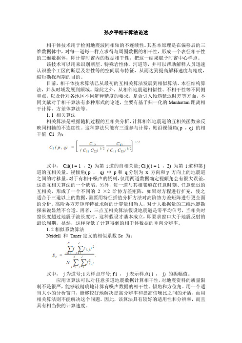
这种算法只能有三道参与计算,则沿视倾角( p ,q) 的相干值C1 为:式中,Cii( i = 1 ,2) 为第i道的自相关量; Ci j( i = 1 ,2) 为第i道和第j 道的互相关量。
视倾角( p ,q) 中p和q分别为x 方向和y 方向上的地震道之间的时移量。
对于有相干噪声的资料,仅用两道数据确定视倾角会有很大误差,这是互相关算法的一个缺陷。
另外,每一道与其相邻道在任意时刻、任意延迟的互相关,形成了一个不同的 2 ×2 阶协方差矩阵,如果对方程进行扩充,使之适合于三道以上的数据,需要用特征插值分析方法对高阶协方差矩阵进行更全面的分析。
高阶协方差矩阵特征求解的计算量相当大,对于大数据量的三维地震勘探来说显然不合适。
再者,三点互相关算法假设地震道是零平均信号,当相关时窗长度超过地震子波长度时,这种假设才基本成立,即要求窗口大于地震反射的最长周期,显然,这样降低了计算得到的相干体数据的垂向分辨率。
1. 2相似系数算法Neidell 和Taner定义的相似系数Sc 为:式中,j为道号; i为样点序号; f i ,j表示样点( i ,j) 的振幅值。
coherent相干公司的介绍
Coherent公司是一家总部位于美国加州的全球领先的激光技术公司。
该公司成立于1966年,是激光技术领域的先驱和创新者,致力于开发、制造和销售各种激光器、光学元件和激光系统,以满足科研、工业、医疗、通信等多个领域的需求。
公司历史Coherent公司始于1966年,最初是由一个名叫詹姆斯·汉森(James Hobart)的物理学家和一群斯坦福大学的研究人员共同创立的。
最初,公司主要从事激光技术的研究和开发工作,随着时间的推移,逐渐成为全球领先的激光技术公司之一。
技术创新Coherent公司在激光技术领域拥有丰富的技术积累和创新能力。
该公司的产品涵盖了各种激光器、光学元件和激光系统,包括固态激光器、半导体激光器、气体激光器、飞秒激光器等。
这些产品在科学研究、工业制造、医疗诊断和治疗、通信等领域都有广泛的应用。
应用领域Coherent公司的产品被广泛应用于各种领域:科学研究:用于物理学、化学、生物学等领域的实验和研究。
工业制造:用于激光切割、激光焊接、激光打标等工业生产过程中的精密加工。
医疗诊断和治疗:用于激光手术、医学成像、激光治疗等医疗应用。
通信:用于光纤通信系统中的光源和调制器件。
全球影响力Coherent公司拥有全球范围内的销售和服务网络,在美国、欧洲、亚洲等地设有分支机构和办事处,为客户提供及时、专业的技术支持和售后服务。
该公司的产品和解决方案已经在全球范围内得到广泛应用,并赢得了客户的信赖和好评。
社会责任作为一家全球性企业,Coherent公司积极履行社会责任,致力于环境保护、员工福利和社区发展。
该公司通过采取节能减排、资源循环利用等措施,努力降低环境影响。
同时,Coherent还支持员工培训和教育项目,并积极参与社会公益活动,推动科技进步与社会发展的融合。
总的来说,Coherent公司以其丰富的激光技术经验、广泛的产品线和全球化的影响力,成为了全球激光技术领域的领先企业之一,为推动科技进步和社会发展做出了重要贡献。
三维相干体技术在断裂系统解释中的应用

三维相干体技术在断裂系统解释中的应用摘要随着复杂断块油气田的勘探进一步深入,地震解释技术和地震属性技术都有了长足的进展。
然而常规技术对于复杂构造的描述难以取得很好的效果。
对于断裂系统比较复杂的地区,利用三维相干体技术识别复杂构造和低序级断层是行之有效的一种方法。
关键词构造;三维相干体;断裂系统中图分类号te1 文献标识码a文章编号1674-6708(2010)21-0144-01三维相干体技术是通过比较局部地震道波形的相似性、求异存同、突出波形的突变点,利用三维体切片动态连续显示,达到识别断裂系统以及地质异常体等的目的。
这项技术的应用过程中主观因素较少,解释成果相对比较客观,对于高品质地震资料来说,可以分辨微小断层,监测修正解释结论,提高解释精度。
1相干体算法概述最早的第一代相干算法[1]主要考虑某一道沿cdp方向(x)和测线方向(y)与邻道的相关性。
是基于互相关的相干性算,计算比较简单,在处理有噪数据上存在某些局限性,仅适用于高质量的地震资料。
第二代算法[2]是通过在数学上建立一个协方差矩阵,把主测线和联络测线方向上2道互相关推广到多道分析窗内的多道互相关,并通过沿协方差矩阵中各个检测倾角/方位计算多道相干,其抗噪能力较强,可指示辨认反射面的倾角和方位,有利于识别旋转断块等,但分辨率较低。
相似系数计算的是协方差矩阵全部特征加权求和与全部特征值之和的比。
根据协方差矩阵特征值所对应的物理意义,大特征值代表的是分析元素空间中的主要成分,在有效信号占有的地震道中,它反映的是有效信号;而小特征值代表的是分元素空间中的次要成分,通常是噪声干扰。
仅保留大特征值,去除小特征值,有可能去除噪声干扰,改善相干体计算的分辨率。
根据这一认识,gersztenkorn 等提出了第三代[3]基于特征结构的相干体计算方法。
2 相干参数的选择相干参数的选取,决定着相干体计算的效果。
两个重要参数是相干道数和时窗长度。
地震相干体分析运算中窗口内的道数直接影响到相干体平均效应的大小。
相干体分析技术在BST地区的应用
收稿 日期 :0 1 5 9 2 1 一O —1
作者简介: (95 )女(  ̄ 18- , 汉族)河南省巩义市人,08 , 20 年7 月西南石油大学勘查技术与工程专业本科毕业。 现为西
南石油大学地球探 测与信息技术专 业 20 0 8级的硕士 , 目前主要从事地 震资料 综合解释与地 震属性 提取 与技 术 方 法研 究 。
l 。 Ot
由于工区北部地表为沙漠、 戈壁 , 南部为农 田、
戈壁 和 山地 , 面高程 北低 南高 (5m-80 。地 地 5 0 - 0m)  ̄ 面激发接受条件较差 。工区内除B 3 8 井北三维资料 品质 相对较 好 外 ,Q5井南 、 8 区三维 资 料横 向 S B 3井
和纵 向分辨率均低于 B T连 片其它三维地震资料 , S 且信噪比相对较低 , 连续性差 , 断点不 清晰, 断裂的 平 面组 合存 在 多解 性 , 料 整 体 的可 对 比性 相 对 较 资
9 8
内 蒙古 石 油化 工
2 1 年第 1 期 01 4
相干体分析技术在 B T地区的应用 S
李 倩 朱仕军 文 中平。朱鹏 宇 , , ,
( .西南石油大学 , I1成都 1 l I  ̄J 6 0 0  ̄. 15 0 2 川庆钻探工程有限公司地球物理勘探公司 , 四川 成都 601) 1 2 3
一
震勘探区块 , 满覆盖面积总计约1 2k 。 区钻探 47m。 该 始 于二十世纪 5 年代 , o O 8 年代本 区迎来钻井勘探 的高 峰期 , 18 —1 9 间 , 施 勘 探 开发 井 达 在 9 5 90年 实 到了 2 8口, 占本 轮连 片 区井位 数的 1 2从 上个 世 约 /} 纪9 年代至今 , 0 本区又陆续完成2 o多口井的钻井工 作 。在 5 多 口井的钻探过程中, O 先后发现侏 罗系头 屯河组( 2 井)三工河组 ( 3 井) B7 、 B 4 油藏、 三叠系烧 房 沟组 ( 8 井) 韭菜 园子组 ( 8 井 ) 藏} 中 B0 、 B1 油 其 B 4井 区 于 19 3 97年 上 报 石 油 地 质 控 制 储 量 9 3 1×
三维相干体技术在三维精细构造解释中的应用_吴永平

第15卷第2期2008年3月复杂断块油藏是受众多断层切割、复杂化了的断块圈闭所形成的一类比较特殊的油藏。
在这类油藏中断层是至关重要的组成部分,由于复杂断块油田最突出的地质特点是断层多,断块小,因此,如何精细地构造解释将成为断块油田制定勘探及开发措施的关键[1]。
三维相干体技术是20世纪90年代后期兴起的一项十分有效的地震解释技术[2],利用地震相干体技术在相干切片上能够直观地反映构造和断层的分布情况。
使得断层、特别是小断层进行自动解释成为可能。
三维相干数据的应用方法是MBahorich和SFarmar于1994年提出的,由阿莫科公司组成了CTC(CohereceTechnologyCompany),专门展开这项技术研究,用于识别断层、地层特征及其相互关系,称其为三维相干体。
近几年,国外对三维相干技术这项技术的研究较多[3-4],目前国内对这项技术也有研究[2,5-9]。
文中简单介绍了多道相关技术的基本原理,并以实例说明三维相干技术在构造解释中的应用。
1相干数据体技术原理地震相干是对相邻地震道之间的地震属性(如波形、振幅、频率、相位等)相似程度的测量。
计算地震相干数据体的目的主要是突出那些不相干的地震数据,通过在纵向和横向上分析局部波形得出三维地震相干体的估计而生成的。
在出现断层、特殊地质体的小范围内地震道之间的波形特征可以发生变化,进而导致局部道与道之间的相关性发生突变;突出相邻道之间地震信号的差异性,使断层、相变、岩性异常体以及其他地质现象的不连续性得到低相关值的轮廓。
通过提取三维相关属性体,便可以把三维反射振幅数据体转化为三维相似系数或相关值的数据体。
三维相干体技术在三维精细构造解释中的应用吴永平1王超2(1.成都理工大学能源学院,四川成都610059;2.西南石油局油气测试中心,四川德阳618000)文章编号:1005-8907(2008)02-027-03收稿日期:2007-06-21;改回日期:2007-12-17。
相干反斯托克斯拉曼光谱

相干反斯托克斯拉曼光谱
相干反斯托克斯拉曼光谱(Coherent anti-Stokes Raman spectroscopy,CARS)是一种非线性光谱技术,用于分析物质的分子振动信息。
CARS结合了拉曼光谱和激光非线性光学技术。
在CARS技术中,两个激光光束同时作用于物质样品上。
一个光束是频率高的泵浦光,另一个是频率低的拉曼光。
当这两束光作用于样品上时,它们与样品中的分子振动模式相互作用,产生一个新的频率低于泵浦光的信号,这被称为CARS信号。
通过检测和分析CARS信号的强度和频率,可以获得样品中分子的振动信息。
相比传统的拉曼光谱技术,CARS具有快速、灵敏、非破坏性等优点。
它能够实时获得分子振动信息,不需要显微镜,适用于各种样品类型,包括液体、气体和固体。
CARS技术在许多领域中有广泛应用,包括生物化学、材料科学、环境科学等。
它可以用于分析化学反应动力学、表面催化过程、生物分子结构等的研究。
同时,CARS还可以应用于药物开发、环境监测、生物医学成像等方面的应用。
几种属性原理分析
八 几种典型属性原理及应用
〔3〕基于体属性的相干算法 体属性相干算法实际上是将地震数据体微
分成很多个三维子体进展三维上的分析计 算,这样可以对任意道进展三维体属性以 及相像分析,估算其相干性。 CohTEEC〔第四代相干?〕
八 几种典型属性原理及应用
常规地震剖面和地震属性沿倾向的垂直剖面和断 层与同相轴切割的水平切片比较简洁解释,但是 沿走向的垂直剖面及平行断层同相轴的水平切片 却是很难解释的。
相干体不连续显示较好地解决了这些问题。它能 够准确的反映地下地层的不连续特征,进展定量 断层、岩性特别体和碳酸岩盐缝孔等地质与油气 储集体的解释。
缺点:不能正确反映地层倾角变化
八 几种典型属性原理及应用
〔3〕特征值分析算法C3: 1999年由Gersztenkorn.A.和
Marfurt,K.J.提出的,即通过计算协方差矩 阵的特征值来得到相干属性,C3相干算法 实际上是基于C2算法的协方差矩阵进展三 维地震数据体的相干值计算。可对任意多道 地震数据进展相干计算。 设λi( j=1,2,L,J)是协方差矩阵C的第j个特征 值,其中λi是其最大的特征值。C3相干算法 的计算公式为:
八 几种典型属性原理及应用
首先定义纵测线上t时刻、道位置在〔xi,yi〕 和〔xi+1,yi〕与地震道u之间延迟为L的相互 关系数Cx,下式中 2w为相关时窗的时间长度:
∑ w u(t-τ,xi,yi)u(t-τ-l,xi1,yi)
∑ ∑ Cx(t,l,xi,yi)≡wτw
w
u2(t-τ-l,xi,yi) u2(t-τ-l,xi1,yi)
八 几种典型属性原理及应用
相干计算可以在相干较弱或被噪声干扰的状况下,供给出 数据相像性的定量值。通过对地震数据体相干属性的量化 处理,针对波形进展相干运算,生成新的不同于常规地震 振幅数据体的相干属性体。这种数据体可以用于较为简单 的断层及隐蔽地层岩性的解释,而这些简单的地质特征在 常规地震数据中往往无法识别和解释。
相干体技术
相干体技术相干体技术由相干技术公司(CTC )和Amoco 公司发明,1997年获美国专利,名称为“信号处理和勘探的方法”。
该技术被称为是近几十年来三维地震解释方面的最重要的突破。
与原来揭示地下异常体的方法相比,相干体技术更能清楚地识别断层和地层特征。
相干体技术的特有算法是通过三维数据体来比较局部地震波形的相似性。
相干值较低的点与地质不连续性如断层和地层、特殊岩性体边界密切相关。
对相干数据体作水平切片图,可揭示断层、岩性体边缘、不整合等地质现象,为油藏描述提供识别油藏特征的有利证据。
计算地震相干数据体的目的主要是对地震数据进行求同存异,以突出那些不相干的数据。
通过计算纵向和横向上局部的波形相似性,可惟得到三维地震相关性的估计值。
在出现断层、地层岩性突变、特殊地质体的小范围内,地震道之间的波形特征发生变化,进而导致局部的道与道之间相关性的突变。
沿某一线时间切片计算各个网格点上的相关值,就能得到沿着断层的低相关值的轮廓,对一系列时间切片重复这一过程,这些低相关值的轮廓就成为断面。
同理,地层边界、特殊岩性体的不连续性也产生类似的低相关值的轮廓。
通过三维相关属性体的提取[14],就可以把三维反射振幅数据体转换成三维相似系数或相关值的数据体。
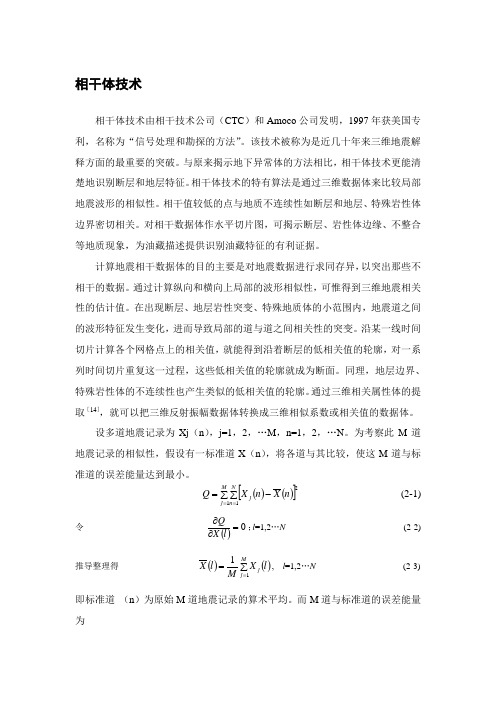
设多道地震记录为Xj (n ),j=1,2,…M ,n=1,2,…N 。
为考察此M 道地震记录的相似性,假设有一标准道X (n ),将各道与其比较,使这M 道与标准道的误差能量达到最小。
()()[]∑∑-===M j Nn j n X n X Q 112(2-1)令()0=∂∂l X Q;l =1,2…N (2-2) 推导整理得 ()()∑==Mj j l X M l X 11, l =1,2…N (2-3)即标准道 (n )为原始M 道地震记录的算术平均。
而M 道与标准道的误差能量为()()[]()()()()[]∑∑+-=∑∑-=====M j Nn j j M j Nn j n X n X n X n X n X n X Q 11221122()()∑∑∑-====M j N n Nn jn X M n X 11212(2-4)此误差能量Q 与M 道地震记录总能量之比为()()()()()()∑∑∑-=∑∑∑∑∑-=∑∑==========M j Nn j Nn M j Nn j M j N n Nn jM j Nn j n X n X M n X n X M n X n X Q 11221112112121121 (2-5)称为M 道地震记录的相对误差能量。
深水浊积水道体系构型模式研究_以_省略_尼日尔三角洲盆地某深水研究区为例_林煜
005 、 2011ZX05009003 ) 和国家自然科学基金青年基金项目( 编号 40902035 ) 的成果。 注: 本文为国家科技重大专项( 编号 2011ZX050301217 ; 改回日期: 20130322 ; 责任编辑: 黄敏。 收稿日期: 20121985 年生。博士研究生。主要从事精细油藏描述及开发地质研究。Email: lin66yu@ 163. com。 作者简介: 林煜, 男,
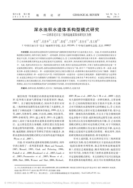
图 3 单一水道的平面形态( 底图为研究区 某准层序内部相干体切片) Fig. 3 Plane shape of single turbidity channel ( The base maps are the slices of coherence cube inner a subsequence of study area)
3
单一水道构型模式
关于单一水道的构型模式, 笔者主要从几何形 态、 定量规模、 平面砂体分布和内部充填样式几个方 面开展了研究。
图 4 尼日尔三角洲盆地深层局部密井网单一水道构型解剖成果 Fig. 4 Architecture characterization result of single turbidity channel using dense spacing well data of deep strata in the Niger Delta Basin
( a) 顺直型; ( b) 弯曲型 ( a) straight type; ( b) bending type
图 2 尼日尔三角洲盆地浊积水道体系构型级次划分 Fig. 2 Hierarchical division of turbidity channel system in the Niger Delta Basin
Paradigm (CORELab)相干属性手册
77 Coherence CubeContentsCoherence CubeOverviewThe Coherence Cube quantifies the measurement of local waveform similarity withina “global” aperture defined in space and time, utilizing dip and azimuth calculations.The process provides accurate maps of the spatial change in the seismic waveform thatcan readily be related to geologic features and depositional environments. Faults andfracture systems can now be spatially imaged and directly mapped from the CoherenceCube without the tedious and extremely subjective method of interpreting faults onselected vertical sections,then connecting the interpreted segments to give a completefault picture. Depositional systems can be more readily understood as the processhighlights such depositional features as channels,onlap,turbidite sequences,etc.Thequality of the Coherence Cube result depends upon selection of optimum processingparameters specifying dip constraints, temporal and spatial aperture and processingalgorithms.In addition to the coherence attributes derived by Eigen and Semblance, processingseveral multi-trace attributes may be derived via the Hilbert transform. Theseattributes (frequency, phase amplitude and dip attributes) can often help inunderstanding the geologic causes for the coherence variations.Getting StartedYou can access the Coherence Cube application from the Session Manager window.1.In the Session Manager click the Accessories tab and select Coherence Cube.2.The Project/Survey Selection dialog box appears. Select the desired survey, or theproject that contains your survey. Select the survey you want to specify as the active one and click Open.Note:The Project/Survey Selection dialog box does not appear if you have already selected an active project/survey.3.The Open File dialog box appears. Select an input seismic file. The selected filehighlights and the OK button becomes available. Click OK.4.The Coherence Cube Parameters dialog box appears.5.Set parameters as described in the various Coherence Cube Parameters Dialog Boxtables on the following pages.Note:You must specify the output datasets in Output Datasets to run the application.6.Click Run.Note:Selecting the Close button will close the application.Coherence Cube Parameters Dialog Box with Dip Parameters SelectedTable 77-1: The Coherence Cube Parameters Dialog Box - Dip ParametersField/Option DescriptionDip Method Select the Dip Method. The choices are: Bins, FX, and UserDefined.Dip Bins The Dip Bins method is the default.Number of dip/azimuth bins Enter the number of dip/azimuth bins.The higher the number of dip/azimuth bins givesbetter results, especially when the dip is in many different directions, but takessignificantly longer to process.Inline Maximum Dip (msec/trace)Enter the maximum reflector dip observed on the inlines—units are z-units per trace,unsigned real number.Xline Maximum Dip (msec/trace)Enter the maximum reflector dip observed on the crosslines—units are z-units pertrace, unsigned real number.FX Dip Parameters The FX Dip method is used to reduce dip banding that may be imparted by the binsmethods.Since it is a gated method,it should not be used when the true dip changesrapidly vertically, for example when the target is at an angular unconformity.FX Dip Half Aperture (traces)Increasing this to3or4traces half-aperture may give a more stable dip estimate if thedata is noisy, but the runtime will increase.User Defined Dip Parameters The User Defined Dip method is used when more dip control is needed than producedby the standard bins method.It is usually used for specific targets rather than for entiredatasets. The dip values are explicitly honored, that is there is an asymmetricdistribution of dip bins. Dip value is positive if event time increases as trace numberincreases, and negative if event time decreases as trace number increases. Number of Dip Bins This is a non-linear scalar to increase or decrease the number of dip bins calculated.Increase the number to obtain more bins, reduce it for fewer bins.Minimum Inline Dip (msec/trace)Enter the minimum reflector dip on the inlines in z-units per trace. This is a signed realnumber - usually a negative number.Maximum Inline Dip (msec/trace)Enter the maximum reflector dip on the inlines in z-units per trace.This is a signed realnumber - usually a positive number.Temporal ApertureThe Temporal Aperture (or window length)is the most critical parameter,and most of the testing involves getting the best temporal aperture for the dataset. The results suggest that best temporal aperture ranges from about one-half wavelength of the highest frequency to about one times wavelength of the lowest frequency of the reflection data. Longer temporal aperture may be used to suppress noise in the coherence result, but short-lived events such as channels are obscured with longer operators.In general,smaller apertures should be used when attempting to highlight stratigraphic features or very low angle faults,and longer apertures should be used to highlight features that are more persistent vertically, such as high-angle faults.Coherence Cube Parameters Dialog Box With Temporal Aperture SelectedMinimum Xline Dip (msec/trace)Enter the minimum reflector dip on the crosslines in z-units per trace. This is a signed real number—usually a negative number.Maximum Xline Dip (msec/trace)Enter the maximum reflector dip on the crosslines in z-units per trace. This is a signed real number—usually a positive number.Table 77-2: The Coherence Cube Parameters Dialog Box - Temporal ApertureField/OptionDescriptionSemblance half-aperture length in samplesEigen half-aperture length in samplesEnter the half-aperture for both the Semblance and Eigen operation.A half-aperture of 5indicates that 5samples above and 5samples below the center for all the traces in the aperture will be used in the calculations. This would result in a 40 milliseconds temporal aperture for Sample Rate = 4 ms.Separate values may be entered,for example,a larger number of samples might be entered for the semblance half-aperture in order to provide a more stable dip estimate. Normally they are the same.Table 77-1: The Coherence Cube Parameters Dialog Box - Dip ParametersField/OptionDescriptionSpatial ApertureSpatial Aperture is specified either as rectangular or circular. Increasing the number of traces may reduce noise, but it takes longer to process, and may also result in smearing the data since additional traces are further away.Coherence Cube Parameters Dialog Box with Spatial Aperture SelectedCoherence Output ScalingThe coherence output values normally range between 0 and 1.0 where 1.0 represents identical traces. The scaling capability allows the user to linearly scale the data to -128.0to +127.0so that there is no need to rescale data while loading to interpretation systems. Additionally, traces are always somewhat like their neighbors, with typical values are between .5 and 1.0, so the result may be “debiased” to retain optimumTable 77-3: The Coherence Cube Parameters Dialog Box -Spatial ApertureField/OptionDescriptionInclude Diagonal traces Toggle on Include Diagonal traces to include traces which are not on the same line or crossline as the central trace.Spatial Aperture Type Select Rectangular or Circular.Rectangular ApertureHalf-Aperture of 1 indicates that one trace on each side of the trace beingcalculated will be used, along with the central trace. Typical apertures are one to three traces on each side, both inline and crossline. Also toggle on the IncludeDiagonal traces to include traces which are not on the same line or crossline as the central trace.For the example above 5traces will be used,one from each side of the center trace in both the inline and crossline directions.Inline Half Aperture (traces)Enter the number of traces of the inline from each side of the center point.Xline Half Aperture (traces)Enter the number of traces of the crossline from each side of the center point.Circular ApertureCircular Aperture Radius (survey working units)Enter the radius in feet or meters.dynamic range. For example, a value of .5 would be -128 and a value of 1.0 would be127.0 Data below 0.5 would be clipped to -128.0.An optional scaling factor is also provided to non-linearly scale the coherence data.This option is provided in order to spread out high coherence values more than lowcoherence values, and may be useful in showing variations which may be related todepositional features (on lap, etc.) or fluid contacts.The following table shows the values after exponentiation and linear scaling for arange of calculated values.Table 77-4: Table 1: Coherence Cube Output ScalingCoherence Output ValueValue Afterexp - 1(default)Value AfterLinear ScaleValue Afterexp = 1.5Value AfterLinear ScaleValue Afterexp = 2Value AfterLinear ScaleValue Afterexp = 3Value AfterLinear Scale 00-1280.00-128.000-1280-1280.10.1-102.50.03-119.940.01-125.450.001-127.745 0.20.2-770.09-105.190.04-117.80.008-125.96 0.30.3-51.50.16-86.100.09-105.050.027-121.115 0.40.4-260.25-63.490.16-87.20.064-111.68 0.50.5-0.50.35-37.840.25-64.250.125-96.125 0.60.6250.46-9.490.36-36.20.216-72.92 0.70.750.50.5921.340.49-3.050.343-40.535 0.80.8760.7254.460.6435.20.512 2.56 0.90.9101.50.8589.720.8178.550.72957.895 11127 1.00127.0011271127Coherence Cube Parameters Dialog Box with Coherence Output Scaling SelectedTable 77-5: The Coherence Cube Parameters Dialog Box -Coherence Output ScalingField/Option DescriptionMinimum Coherence Output Value Enter the minimum coherence output value.Maximum Coherence Output Value Enter the maximum coherence output value.Debias Coherence Minimum Enter the debias coherence minimum value. Data below this value will be clipped. Debias Coherence Maximum Enter the debias coherence maximum value. This value is rarely modified.Output Scaling Factor Enter the output scaling factor.Adaptive Eigen ParametersThe Adaptive Eigen parameters allow for strong noise reduction while maintaining theimportant low coherence features. Supply High for Adaptive Smoothing and High forAdaptation Rate for the greatest noise reduction. If the result has an “artificial” look,you should first reduce the Adaptation Rate,then the Adaptive Smoothing parameterif required. The default is for no adaptive processing.Coherence Cube Parameters Dialog Box with Adaptive Eigen Parameters SelectedTable 77-6: The Coherence Cube Parameters Dialog Box -Adaptive Eigen ParametersField/Option DescriptionAdaptive Eigen Processing Toggle on Adaptive Eigen Processing to get adaptive processing.Adaptive Sampling The choices are: None, Low, Medium, and High.Adaptive Smoothing The choices are: None, Low, Medium, and High.Adaptive Rate The choices are: None, Low, Medium, and High.High Resolution ParametersThe High Resolution parameters are Eigen and Semblance outputs are “sharpened”versions of the Eigen and Semblance, respectively. The sharpening is performed witha Laplacian operator, typically applied on a horizontal slice, that is, the output valueof any sample is based on the local neighborhood of adjacent traces.Coherence Cube Parameters Dialog Box with High Resolution Parameters SelectedTable 77-7: The Coherence Cube Parameters Dialog Box - High Resolution ParametersField/Option DescriptionHigh-Resolution Method The sharpening is commonly performed on horizontal slices, but you may selectvertical, in which case the sharpening will be performed on inlines.High-Resolution Sharpening Select Low, Medium, or High.Advanced ParametersCoherence Cube Parameters Dialog Box with Advanced Parameters SelectedTable 77-8: The Coherence Cube Parameters Dialog Box - Advanced ParametersField/Option DescriptionAdaptive Smoothing Value (0 - 1.0)This parameter is used if the user desires more smoothing than given with the Adaptiveparameters. A value of 1.0 provides the greatest amount of smoothing, with 0providing no smoothing.Seismic Resample (1 - 4)In conventional coherence processing, trace data is resampled to(SR/4) value toreduce aliasing, that is, sample rate of 4 ms is resampled to 1 ms or sample rate of 2ms is sampled to 0.5 ms. A very large memory requirement (very long lines) may bereduced by making the Seismic Resample smaller than 4; however, more aliasing ispossible. This parameter should not be changed unless the data is very flat, and thememory reduction is required to make the program run.FX Dip Half-Gate (8, 16, 32,64)The trace data is divided into n gates of length 2 * half-gate samples. A single dipvalue is calculated for each window and is applied to every sample within the gate.Shortening the FX Dip Half-Gate may result in a better geologic representation(i.e.,alldips in the window are the same), but it results in a less accurate frequencyrepresentation. This parameter should be used with caution. The default value is 16.High-Resolution Sharpening Value (.001 - 1.0)This parameter is used if the user wants more or less sharpening than provided by the high resolution parameters. A value of .001 provides the least sharpening and 1.0 provides the most sharpening.Eigen Aperture Enter All or Center 5. Eigen calculations are performed using All traces in the SpatialAperture or only the Center 5 traces. Default is All.Re-apply Start Times Mute This toggle can be used to reapply a mute at the input data start times. This is usefulin cases of rapidly changing water bottom.Output Volume LimitsSelect the appropriate parameter to process a subvolume of the entire dataset.Coherence Cube Parameters Dialog Box with Output Volume Limits SelectedTable 77-9: The Coherence Cube Parameters Dialog Box - Output Volume LimitsField/Option DescriptionInline LimitsFirst Inline Output Enter the first inline to be output.Last Inline Output Enter the last inline to be output.Inc Inline Output N/AXline LimitsFirst Xline Output Enter the first xline to be output.Last Xline Output Enter the last xline to be output.Inc Xline Output N/ATime LimitsStarting Time Enter the starting time of the subset you wish to process.Ending Time Enter the ending time of the subset you wish to process.AzimuthOutput Datasets1.Click on the Select button to select a file name,file organization,and format.Youmay process any or all of the output datasets in the same run.The Create Output File dialog box appears.2.You can accept the default Logical Name and Comment names or provide yourown Logical Name and Comment name. Also, you can modify the Output Formatand Organization. You must select each file that you want to output.3.Click New . Click Run in the Coherence Cube Parameters dialog box.Inline AzimuthThis parameter is the direction of increasing crossline numbers on an inline.This shouldonly be modified if dip/azimuth volumes are to be output as absolute values. 0degrees is due north, 90 degrees is east, 180 degrees is south, and 270 is east.Xline Azimuth This parameter is the direction of increasing line numbers on a crossline.Input Spacing Inline Spacing N/AXline SpacingN/A Table 77-9: The Coherence Cube Parameters Dialog Box - Output Volume Limits (Continued)Field/OptionDescriptionCoherence Cube Parameters Dialog Box with Output Datasets SelectedHintYou will probably create quite a few datasets.It is useful to modify the defaultLogical Name to reflect the processing parameters, e.g., for processingparameters with Temporal Aperture +/-5 samples, and Spatial Apertureadjacent traces, the output name might be Eigen 5 sample 5 trace.A processing log is written in the xterm and a Work In Progress window is written tothe screen.You may stop the processing at any time.The partial datasets created are automatically saved, so data may be viewed immediately. These datasets may beoverwritten by subsequent runs, if desired, or they may be deleted using the FileManager from the Session Manager.The processing log contains useful information about the job as it is running. First alisting of the processing parameters is given. You may verify that the processingparameters are as expected.If not,you can stop the job,fix any problems and start from the beginning,if necessary.When processing has completed amplitude ranges for each output volume are listed inthe log, as well as the percentage of data which falls into each dip-azimuth bin. The“hit” distribution gives some indication of the “quality” of the dip-sampling, forexample,a list with many empty bins may show that the dip-azimuth is oversampled,and a better result might be obtained with different Dip parameters.Run times allow you to estimate run times for future runs. Amplitude minimum/maximum give you an indication that there may be problems with scaling forvisualization, e.g., Instantaneous Envelope Range of 0 1.0e10 suggests there will bedynamic range problems if output data is 8-bit integer.Running the Coherence CubePreconditioning the inputFiltering and ScalingThe Eigen outputs are relatively insensitive to amplitude so scaling has little effect onoutput coherence.Bandpass frequency filtering can make a difference in the coherenceoutput, however, the multi-sample, multi-trace aperture is already a very goodsuppressor of random noise, so bandpass filtering rarely makes a significant impact within the seismic frequency range.Acquisition FootprintUsers are often surprised at the magnitude of the acquisition footprint on the coherence result. While it appears to diminish in the seismic amplitude volume with depth, there are still present small systematic distortions of the seismic wavelet throughout the record. Coherence Cube highlights these changes; often they are the same order of magnitude as the target wavelet distortions related to faults and stratigraphy.In fact the periodicity is often measurable on the time slices and this measurement can be used to design predictive filters for noise removal.Reduction of the acquisition footprint before Coherence Cube processing usually helps the interpreter to understand the lateral coherence changes.FXY DeconFXY decon or other continuity enhancers run prior to Coherence Cube can produce better results in noisy data.In many cases;however,the adaptive process produces as good or better result.Non-zero Mean InputCoherence Cube is the measurement of the trace to trace changes in the input waveform with the assumption that the input data is zero-mean (such as seismic amplitude). Non-zero mean data, e.g., acoustic impedance, may need debias prior to computing coherence. This capability is not included in this software.Dynamic Range, Format and Display of Output DataYou should pay some attention to dynamic range of both the input and output data. Input data which has been heavily clipped when it was converted to 8-bit for display will produce an inferior result to non-clipped data. Input data which has been significantly“integerized”may also produce an inferior result,e.g.,seismic amplitude data with a range+/1.0e08divided into the255bins for8-bit processing results in just 255 numbers which are 392,156 apart, which is a significant loss of accuracy. Coherence Cube output data is by default set to integer ranges. There is no loss of accuracy when outputting this data as8-bit.The attribute data may;however,show a loss of accuracy.The internal scaling performed during output assumes a symmetrical distribution of the data. The example above would produce an output Instantaneous Amplitude Envelope between0and1.0e+08.However,the output would be converted to 255 bins between - 1.0e+08 and + 1.0e+08; that is only 126 bins to define the true data range. It is recommended to output this data as 16 or 32 bit float format.Run Rates vs ParametersTotal run time for the Coherence Cube is highly dependent upon the parameters selected. The most significant impact to runtime is the number of traces in Spatial Aperture. Increasing the number of traces in the Spatial Aperture increases the run time, although fast processing paths are provided for 5 trace or 9 trace apertures. Increasing the sampling of the dip bins also significantly impacts the run time since it increases the number of semblance calculations which must be performed.The FX Dipmethod run time usually falls somewhere between the medium and high dip samplerun times for the same number of traces. Adaptive processing increases run times by30to40percent.Increasing the number of samples in the Temporal Aperture has littleimpact on runtime, and the addition of the High Resolution Parameters output alsohas little impact.Addition of Hilbert transform attributes only has a modest impact ontotal run time.The very fastest run time which can be achieved is semblance only, zero dip bins, Dipmethod, 5 trace, non-adaptive processing. This rarely produces the optimum qualityoutput.Analysis of ResultsResults must be analyzed in a visualization system, such as VoxelGeo or ReservoirNavigator. Traditionally, a gray scale color table is used with white representinghighest coherence and black representing lowest coherence.It is important to realize that,unlike features typically observed on seismic amplitudedatasets, the low coherence lineations may only be a few traces wide. Visualcompression of large datasets (i.e., zooming out) may completely misrepresent lowcoherence lineations because those traces are not displayed.Coherence Cube’s greatest advantage lies in highlighting the lateral extent of faults,channels,and other features.For this reason,more attention is necessary for the timeor horizon slices rather than vertical sections.Co-rendering of the seismic amplitude and Coherence Cube is a valuable tool withwhich to analyze results.Typical Testing Sequence1.Run VoxelGeo or Reservoir Navigator.Scan the volume and measure the maximumdip inline and crossline. Select an area(s) for parameter testing.2.Run the first job with+/-5samples,5trace aperture,low or medium dip sampling.Output Eigen, semblance, and high-resolution Eigen.3.Run two more jobs with lower and higher vertical aperture, same dip and spatialparameters as previous job. Output Eigen only.4.VoxelGeo or Reservoir Navigator determine best vertical aperture and whichoutputs are going to be useful.5.Run a9-trace job with best vertical aperture,same dip and spatial parameters asprevious job, Eigen only output.6.Run a test for better dip estimation, best vertical and temporal aperture.—If excessive dip banding shows in steep dip areas, run FX Dip method.—If high coherence areas seem gray rather than white, run with higher dipsampling.—If steepest areas are aliased, use higher dip maxima.If lots of areas show dark low coherence noise especially around faults, testadaptive processing with high samples,high smoothing,and high rate,low sample,high adaptive, and high rate.Technical InformationWaveform similarity is calculated along dipping planes which pass through the samplebeing computed. The local planes contain the traces described by Spatial Aperture.The waveform differences between the traces in the local plane are calculated over atime range centered at the sample being computed.Interpretive input is not requiredresulting in an unbiased calculation of waveform similarity.Several methods are provided to compute the dip. The standard method is the Binsmethod in which trial bins are computed and semblance measured for each trial bin—the bin with the highest semblance value is assumed to have the correct dip and dip-azimuth. The user must supply the maximum dip for the inline and the crosslinedirection in msec/trace (only the maximum of these, in msec/meter or msec/foot, ispassed to the program), as well as a dip-sampling factor. Dip/azimuth bins aregenerated symmetrically for both the inline and crossline,that is if a value of4.0is thedip maximum,dip maxima will range from-4.0to+4.0in both the inline and crosslinedirections. The dip sampling factor controls the number of dip bins calculated. Thelow sampling is sufficient for most areas;however,the Dip Sampling factor should beincreased for steeply dipping data,and for data with many different directions of dip.The bins dip is allowed to vary from sample to sample,trace to trace,and thus producesa very good local dip estimate; however, for steeper dips there is often a dip bandingeffect along the inflection points of the wavelet.This banding can obscure some events,and so the second method is a FX dip estimation which is estimated over longerwindows of the trace, resulting in a more stable dip estimate; thus eliminating somebanding.This method uses a gated Fourier transform then measures the phase changein the frequency domain.The third method is to supply actual signed dip ranges for inline and crosslinedirections. Sign value convention: positive value for time increasing as trace (or linenumber) increases; negative value for time decreasing as trace (or line number)increases.This computes dip bins asymmetrically,honoring exactly the limits the userhas specified.Semblance is one measurement of waveform similarity calculated for each dip bin.Thedip bin with the highest semblance value is assumed to be the correct one, thesemblance value is output to the semblance file,and the dip bin is passed to the Eigenalgorithm.The Eigen algorithm outputs another measurement of waveform similarity using amulti-trace Eigen decomposition process which is more robust and has higherresolution than other measurements, including semblance. Consider two seismictraces whose amplitudes are crossplotted sample by sample on the Cartesiancoordinate system. The distribution of the general shape of the plotted points can berepresented by an ellipse and the pattern formed by these points is governed by thecoherence of the two input traces plotted.The ellipsoidal shape is not a measure of theindividual samples but more a measure of the overall waveform shape being input.Consider two traces with identical waveforms being plotted on a Cartesian coordinatesystem, described above. The plotted points lie along a straight line running 450through the origin. The ellipse, which describes these points, has a major axis lengthrelated to the maximum excursions on the trace.The minor axis has a value of zero.Ifwe now reverse the polarity of one of the waveforms and replot the points,again theylie on a straight line passing through the origin.If we now fit an ellipse to these pointswe see again that the magnitude of the axes are the same except the direction of themajor and minor axes has a 900 rotation. Thus, we can relate the length of and theorientation of these axes to the similarity of the two plotted input trace segments.Bothorientation and length of the major and minor axes describe the ellipse, which is controlled by the geometry of the two input traces. The directions and magnitudes of the major and minor axes of the ellipse can be represented by two scaled vectors,where the longer vector lies along the major axis and the shorter the minor axis. Mathematically the magnitudes of these two vectors correspond to the two Eigen values of the data covariance matrix and the normalised vectors correspond to the Eigen vectors.The coherency measurement output to the Eigen file is a ratio of the two eigen values.The Eigen decomposition process is only performed for the optimum dip bin.High Resolution Eigen and High Resolution semblance are calculated after the initial Eigen and semblance calculations. A Laplacian unsharp masking operator is applied on each sample of each time slice using a weighted average the adjacent traces on that time slice. The user can control the level of sharpening.Adaptive processing may be applied as the seismic data is read in to the covariance matrix. In the Kuwahara method of noise reduction, statistical measurements are calculated for local regions along the optimum dip plane. The central sample is replaced by the average of the region with the highest similarity.Coherence Cube provides for the computation of multi-trace Hilbert transform attributes.These are similar to conventional single trace Hilbert transform attributes except they are generally smoother since they are computed from a dip-consistent average of all the traces in the spatial aperture.ReferencesMarfurt, et al, 1998. 3-D seismic attributes using a semblance-based coherency algorithm. Geophysics, Vol 63 No4(July-August) pp 1150-1165.Marfurt, et al 1999. Coherency calculations in the presence of structural dip Geophysics. Vol 64 No 1 (January-February) pp 104-111.。
解释模块功能介绍
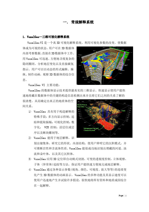
一.常规解释系统1.VoxelGeo—三维可视化解释系统VoxelGeo VI是一个真3D可视化解释系统。
利用可视化参数的改变,使数据体成为可视的状态,用户可在3D数据体内部考察数据,直接在3D数据体中工作。
用VoxelGeo可迅速、方便地寻找复杂的隐闭圈闭、分析地层变化以及直接碳氢指示。
用户可以以动态的形式编辑、操纵、制作动画,观察3D数据体的综合信息。
VoxelGeo VI 主要功能:VoxelGeo的数据体显示技术提供最真实的三维显示。
快速显示使用户能快速地将藏在数据体中的关键的构造信息检测出来并且将它们之间的关系了解的很清楚。
从而确定出真正的地质体的空间关系。
1)VoxelGeo具有用于构造解释的特殊手段:多方向显示控制;追踪和提取振幅;可视化控制;数图3 数据三维显示字化; VCR控制;沿层位或层序以及断块雕刻等。
2)VoxelGeo能用于地层解释,识别出储集体,研究它的形状、内部结构,使用户辨明它的沉积模式,并可推断岩性和含流体性质。
VoxelGeo能很成功地识别出埋藏的河道、浊流和朵叶体,以及其它沉积体。
3)VoxelGeo应用3D定位即自动椅式切割,可变的透视度控制,立体观察,子体 (异常体)追踪等方法,保证用户能快速方便地完成地层解释。
4)VoxelGeo通过各种显示参数(视角、颜色、可视度、放大等等)的连续变化产生3D数据体的动画显示。
VoxelGeo的多种功能及其显示速度可以使用户迅速地产生并试验许多假设,很快地将所有资料和地质成因综合在一起解释。
2.SeisEarth XV—基于体的三维可视化解释系统SeisEarth XV 是基于体的三维可视化解释系统,包括SeisEarth LI+ 、Reservoir Navigator、3D Propagater产品及模块其中:SeisEarth-是基于线的地震解释系统,在合成地震记录、井震标定、2D/3D联合解释、剖面的各种显示方式等功能上都更加强大和方便,并且SeisEarth与 VoxelGeoXV等体解释软件有非常好的结合,从而使构造解释工作更加容易和精确。
相干傅里叶散射测量
相干傅里叶散射测量
相干傅里叶散射测量(Coherent Fourier Scatterometry)是一种
光学表面形貌测量方法,通过测量光的散射模式来获取目标表面的形态信息。
这种测量技术基于傅里叶光学的原理,通过投射一束相干光线照射在目标表面上,光线经过散射后根据散射模式的变化来获得目标表面的形貌数据。
相干傅里叶散射测量将目标表面视为一个散射对象,其形状和物理特性可以通过测量和分析散射数据来推断。
在测量过程中,需要先确定目标表面的散射模式,通常通过改变入射光的波矢方向或入射角度来实现。
然后,测量仪器将记录散射光的强度和相位信息,并以此为基础来重建目标表面的形貌。
由于相干傅里叶散射测量是一种非接触性的测量方法,因此适用于各种表面材料和形态的测量,如光学元件、纳米结构等。
该测量技术在光学制造、光刻技术等领域具有广泛的应用价值。
它可以用于表面形貌的检测和质量控制,帮助确定光学元件的性能和几何参数。
此外,相干傅里叶散射测量还可以用于纳米结构的表面形貌测量和纳米材料的机械性质研究等方面。
总之,相干傅里叶散射测量是一种基于光学散射原理的表面形貌测量方法,通过测量和分析散射模式来重建目标表面的形状和特性。
它在光学制造、纳米技术等领域具有重要的应用价值。
相干光模块原理
相干光模块原理
相干光模块(Coherent Optical Module)是一种用于光通信的装置,它可以将传输的光信号转化为电信号进行处理,并将处理后的电信号转化为光信号再次传输。
相干光模块中的关键技术是光学相干检测技术,它可以通过对光信号的幅度和相位的检测,实现高速、高精度的光信号检测和处理。
相干光模块的工作原理是基于激光器产生的相干光源。
在传输过程中,光信号将经过光学调制器进行调制,然后被光学相干检测器接收和检测。
在光学相干检测器中,光信号被拆分成两路,分别经过两个相位不同的光路,然后再将两路光信号合并进行检测。
这样做的目的是通过比较两个光路的相位差异来获得光信号的幅度和相位信息。
通过这种方式,相干光模块可以实现高速、高精度的光信号检测和处理。
在光通信系统中,相干光模块具有重要的作用,可用于光纤通信、光通信网络、光功率测量等领域。
例如,在高速光通信网络中,相干光模块可以用于对光信号的调制、放大和检测,从而实现高速、稳定的信号传输。
此外,在光通信系统中,相干光模块可以用于对光信号进行精细的分析和测量,从而帮助优化光通信系统的性能。
总体来说,相干光模块是一种基于光学相干检测技术的高精度、高速的光信号处理装置,具有广泛的应用前景。
地震相干技术

C2算法特点
C2算法引入了协方差矩阵,使其可对任意道数进行相似分析,估计其相干性。C2 相干算法除了在噪声环境下更稳健地测量相干之外,垂直分析时窗能被限制在只有几 个时间样点范围内,能够精确做出薄而小的地层特征图。优点:稳定,抗噪性强,一 定范围的可变时窗;不能反映地层倾角。
C3算法特点
C3相干算法借助C2相干算法中引入的协方差矩阵来实现,其分辨率较C1C2算法更高。
数据,由纵向和横向上局部的波形相似性可以得到三维地震相
关性的估计值。
Hale Waihona Puke 相干技术的原理|地震相干数据体的算法比较|相干计算的模式选择和时窗大小选择
一般情况下,现在所作的相干都是基 于振幅的计算,利用多道相似性将三维振
幅数据体转化为相关系数数据体,在显示
上强调不相关异常,突出不连续性。它的 前提假设是地层连续的,地震波有变化也 是渐变的,因此相邻道、线之间是相似的。 当地层连续性遭到破坏发生变化时,如断 层、尖灭、侵入、变形等,导致地震道之 间的波形特征发生变化,进而导致局部道
优点:分辨率高,缺点:没有考虑倾角和方位角
改进的体属性算法 改进的体属性相干算法实际上是将地震数据体微分成无数个三维子体进行三维 上的分析计算,这样可以对任意道进行三维体属性以及相似分析,估算其相干性。
举例来说明地震倾角对相干的属性影响 水平扫描 (1-3)种算法进行的是水平的相似性处理
他的缺点是:突出了倾角方向上的断层,消弱了反倾 角方向上的断层
与道之间的相关性表现边缘相似性的突变,
地层边界、特殊岩性体的不连续性会得到 低相关值的轮廓。
桩23-17-20
T2
Ⅰ砂组 Ⅲ砂组
Ⅳ砂组
T6
Z23-17-20南北向地震剖面
- 1、下载文档前请自行甄别文档内容的完整性,平台不提供额外的编辑、内容补充、找答案等附加服务。
- 2、"仅部分预览"的文档,不可在线预览部分如存在完整性等问题,可反馈申请退款(可完整预览的文档不适用该条件!)。
- 3、如文档侵犯您的权益,请联系客服反馈,我们会尽快为您处理(人工客服工作时间:9:00-18:30)。
t z
trace 1
trace 2
crosscorrelation
Value at Zero lag time (z) measure of similarity Zero lag time (t) measure of dip
Algorithm
z3 t3
X
t1 z1 X X X
Za
for normalization
t2 z2
X
t4 z4
C1 Correlation
The Semblance(c2) Algorithm
“Energy of a summed trace divided by the mean energy of the components of the summed trace; equivalent to crosscorrelation zero lag vealue”
Coherence Cube 相干体技术
郎晓玲
2005.5.24
Topics
• • • • • Coherence Cube History Coherence Cube Definition Coherence Cube Uses Coherence Cube Algorithms Coherence Cube Hands-on
The Eigenstructure (c3) Algorithm
High Resolution Enhancement
• Laplacian Edge Enhancement applied on time slices of coherency output • Both signal and noise are boosted
The Eigenstructure (c3) Algorithm
• Decomposition of covariance matrix which contains these samples results in two eigenvalues and two eigenvectors.
• The two eigenvalues correspond to the lengths of the major and minor axes of the ellipse.
+/- 9 samples
+/- 5 samples
Coherence Cube Uses : With Inversion
Conventional seismic Coherence Cube
Coherence Cube Uses: With Inversion
Coherence Cube Uses: With Inversion
Coherence Cube Temporal Aperture
Greater continuity, faults Greater continuity, Channel system
+/-3 samples +/-9samples
Sharp internal details, Channel systems
Coherence Cube Dip Methods
-dip method bins (sign not used, gives symmetric dip bins) -ildip_max #.# msec/trace –cldip_max #. # msec/trace -dip_sample high (options are low, med, high) -dip_method fx (no other parameters required) -dip method bins (sign must be specifed, more exact control) -pmin #.# -pmax #.# (inline dip min and max, msec/trc -qmin #.# -qmax #.# (crossline dip min and max, msec/trc) -dang # (# dip angles)
• Stratigraphic Interpretation
• Structural Interpretation
• Reservoir Characteristics
– With Inversion – With Offset Processing – With Azimuth Processing
identical traces
tr 1 tr2 tr 1
“ 1”
major axis
“ 0”
minor axis
tr 2
The Eigenstructure (c3) Algorithm
different traces
tr 1 tr2
“ 1”
minor axis tr 1
“ 0”
major axis tr 2
semblance
28
44
60
eigen
28
44
Coherence Cube Temporal Aperture
+/-3 samples
Coherence Cube Temporal Aperture
+/-6 samples
Coherence Cube Temporal Aperture
+/-9 samples
Coherence Cube Dip Accuracy
Measured Dip Max 2.2ms/trc
Dip features
Faults
seismic
19 dip bins
Coherence Cube Dip Accuracy
Supplied Dip Max Too Small
Max dip 3msec/trace 19 dip bins
Noise Adaptive Eigen
Coherence Cube Algorithms
semblance
Байду номын сангаас
eigen
Hi-res. eigen
Coherence Cube Critical Parameters
• Temporal Aperture
• Dip Accuracy
• Spatial Aperture
Coherence Cube Dip Accuracy
Supplied Dip Max Too Large
19 dip bins—8.5 dip max
37 dip bins—8.5ms dip max
Coherence Cube Dip Accuracy
Temporal Aperture
_ _ _ _ +/-3 _ _ _ _ _ _ _ _ _
-w=semblance half temporal aperture
-lentgate = eigen half temporal aperture
Trace samples
Coherence Cube Temporal Aperture
Coherence Cube History
相干体是对地震数据道之间相似性的数学描述,能有力指示地层的非连续性。
• 相干体技术原来是Amoco公司的专利,1995年由Amoco公司的Mike Bahorich引进石油勘探业。 • 该技术揭示了波场的空间变化情况,直接从3D地震数据体中定量地得 到断层和地层特征,不受任何解释误差的影响,极大地提高了解释精度, 并能得到很多通常被忽略的重要信息,因而很快得到了广泛认可。 • 1996,相干技术公司(CTC)成功地将相干体技术商业化并拥有该技术 唯一的许可证。 • 1999年,CoreLab公司收购CTC公司 • 2000 Core Lab 从BP Amoco公司购得相干体技术全套专利。 • 2001 1st corporate software license to major oil company • 2004 Paradigm Geophysical acquires Core Lab Reservoir Technology Division, and license to use and sell Coherence Cube software (Core Lab retains IP) • 2005 Coherence Cube integrated into epos environment
Coherency Definition
Measurement of local waveform similarity in a 3D seismic volume which often represent significant geologic changes
Coherence Cube Uses
Extract Coherence at constant time (time slice view)
Coherence Cube Algorithms
• • • • • Correlation Semblance Eigenstructure Dip Estimation Image Processing Enhancements
index trace
dip traces
attributes
The Eigenstructure (c3) Algorithm
trace 1 trace 1 trace 2
trace 2
Crossplot of Trace Amplitude at each sample
The Eigenstructure (c3) Algorithm
Max dip 1msec/trace 19 dip bins