Seasonal dynamics of macrozoobenthos community structure in Xiangxi River

合集下载

牛油果主要病虫害及其防治

热带农业科技Tropical Agricultural Science &Technology 2024,47(1)：6-10牛油果主要病虫害及其防治毛加梅，黄建，付小猛，杨虹霞，郭俊，王自然，岳建强*（云南省农业科学院热带亚热带经济作物研究所，云南保山678000）摘要摘要：：概述世界各地牛油果的主要害虫种类（蝇类、蛾类、蚧类、螨类，半翅目和鞘翅目类）、主要病害种类（根腐病、炭疽病、疮痂病等真菌性病害以及细菌性软腐病和溃疡病）和病虫害防治现状。

近年来国内牛油果种植面积快速扩张，文章提出从科学合理选园、加强检验检疫、合理选种、选择适宜防治措施等方面来预防和防治牛油果病虫害。

关键词关键词：鳄梨；害虫；病害；防治中图分类号：S667.9文献标识码：A文章编号：1672-450X （2024）01-0006-05Main Diseases and Insect Pests of Avocado and the ControlMAO Jiamei,HUANG Jian,FU Xiaomeng,YANG Hongxia,GUO Jun WANG Ziran,YUE Jianqiang *Institute of Tropical and Subtropical Cash Crops,YAAS,Banshan 678000,ChinaAbstract:The major pest species (flies,moths,scale,mites,hemiptera and coleoptera ）,major disease species (fungal diseas-es such as root rot,anthracnose,scab,and bacterial soft rot and canker ）and pest control status on avocados in the world were summarized.In recent years,the planting area of avocado has expanded rapidly in China.This paper puts forward some measurements against avocado diseases and pests from the perspective of scientific and rational orchard selection,strengthening inspection and quarantine,rational seed selection,and selecting appropriate control methods.words Key words::Persea americana ;insects;diseases;control————————————收稿日期：2023-06-25基金项目：云南省重大科技专项计划（202202AE090004）；保山市科技计划项目（2018kj03）作者简介：毛加梅（1987－），女，助理研究员，主要从事果树病虫害研究工作。

新疆巩乃斯河枯、丰水期大型底栖动物群落结构与环境因子的关系

第41卷第5期生态科学41(5): 208–218 2022年9月Ecological Science Sep. 2022 王燕妮, 田伊林, 刘雨薇, 等. 新疆巩乃斯河枯、丰水期大型底栖动物群落结构与环境因子的关系[J]. 生态科学, 2022, 41(5): 208–218.WANG Yanni, TIAN Yilin, LIU Yuwei, et al. The relationship between macrobenthic community structure and environmental factors during dry and wet seasons in the Gongnaisi River, Xinjiang[J]. Ecological Science, 2022, 41(5): 208–218.新疆巩乃斯河枯、丰水期大型底栖动物群落结构与环境因子的关系王燕妮1,2, 田伊林1,2, 刘雨薇1,2, 崔东2, 尚天翠2, 姚付龙2, 张振兴1, 杨海军1,2,3,*1. 东北师范大学植被生态科学教育部重点实验室, 长春 1300242. 伊犁师范大学生物与地理科学学院, 伊宁 8350003. 云南大学生态与环境学院, 昆明 650091【摘要】为探究新疆巩乃斯河的生态状况, 团队先后在2018年10月(枯水期)和2019年6月(丰水期)对大型底栖动物群落和环境因子进行了调查, 分析大型底栖动物群落结构、功能摄食类群、生活类型组成及其与环境因子的关系。

研究河段共采集到大型底栖动物40种, 隶属3门4纲8目27科, 主要以节肢动物门为主, 其中直突摇蚊亚科(Orthocladiinae spp.)、长跗摇蚊族(Tanytansini sp.)、四节蜉属(Baeits sp.)、亚美蜉属(Ameletus sp.)和Cheilotrichia sp.是优势类群。

脑保护熊利泽

Liu YH, et al. Candian J Anesth 2006; 53(2)
The role of adenosine A1 receptor
400 350 300 250 200 150 100 50 0 Control DPCPX
infarct volumn of brain
（mm 3 ）
自由基的作用
300
Infarct volume (mm3)
200
*
100
0
E
F
G
H
Zhang XJ, et al. Can J Anesth, 2004;51(3)
IF=1.108
异氟醚?
最常用的吸入麻醉药！
西京医院6000例/年
如有预处理效应……!
Xiong L, et al. Anesth Analg 2003;96:233-7
HBO预处理
氧自由基
SOD活性 CAT活性
耐受机制
脊髓保护作用
消除缺血再灌注引起的自由基
研究设计：
1. 拮抗CAT或SOD 对脊髓保护作用的影响？
2. 阻断自由基后,CAT和SOD活性变化？
HBO预处理的部分机制
保护
HBO预处理
氧自由基
抗氧化酶活性增强
线粒体 ATP酶维护功能
线粒体
损伤产生
100%
1h/d 3d/5d
O2
Dong HL, Xiong L, et al. Anesthesiology, 2002;96:907-12
Dong HL, Xiong L et al. Anesthesiology, 2002;96:907-12

《2024年阿尔巴斯白绒山羊与绵羊胚胎干细胞培养技术的研究》范文

《阿尔巴斯白绒山羊与绵羊胚胎干细胞培养技术的研究》篇一一、引言随着生物科技的飞速发展，干细胞培养技术已成为生命科学研究的前沿领域。

尤其是胚胎干细胞培养技术，以其巨大的潜力在动物育种、生物医学及畜牧业等方面发挥了重要作用。

本文旨在研究阿尔巴斯白绒山羊与绵羊的胚胎干细胞培养技术，为未来相关领域的发展与应用提供理论基础和技术支持。

二、研究背景阿尔巴斯白绒山羊是一种优质的毛绒山羊品种，其毛发柔软、保暖性强，具有较高的经济价值。

而绵羊作为重要的家畜之一，其肉质和毛质也具有较高的经济价值。

随着遗传学和细胞生物学的发展，利用胚胎干细胞培养技术来提高动物的品质和数量已经成为了一种可行的策略。

三、胚胎干细胞培养技术的原理与现状胚胎干细胞（ES）是一种能够自我更新并分化成多种类型细胞的细胞，因此其在生物学研究和实际应用中具有重要的价值。

目前，胚胎干细胞培养技术已广泛应用于动植物育种、疾病模型构建等领域。

而阿尔巴斯白绒山羊和绵羊的胚胎干细胞培养技术的探索与应用，则是当前的研究热点之一。

四、研究内容与方法本研究主要围绕阿尔巴斯白绒山羊与绵羊的胚胎干细胞培养技术展开。

首先，通过超数排卵和体外受精等技术获取胚胎；然后，对胚胎进行显微操作，分离出内细胞团（ICM），将其培养成胚胎干细胞；最后，对培养的胚胎干细胞进行鉴定和分析，探讨其在遗传学、生理学和分子生物学等方面的应用潜力。

本研究采用的方法包括细胞生物学技术、分子生物学技术以及显微操作技术等。

通过多学科交叉合作，实现了从胚胎获取到胚胎干细胞培养的整个过程的优化与完善。

五、实验结果与数据分析通过本研究，我们成功地从阿尔巴斯白绒山羊和绵羊的胚胎中分离出内细胞团（ICM），并成功培养成胚胎干细胞。

通过鉴定和分析，我们发现这些胚胎干细胞具有较高的纯度和活性，且在遗传学、生理学和分子生物学等方面具有较高的应用潜力。

同时，我们还发现，通过优化培养条件和操作技术，可以提高胚胎干细胞的分离效率和培养效果。

三种常见原生动物对褐潮藻种抑食金球藻(Aureococcus anophagefferens)的摄食

三种常见原生动物对褐潮藻种抑食金球藻(Aureococcusanophagefferens)的摄食陈瑶;杨茜露;何学佳【摘要】微型浮游动物在抑食金球藻(Aureococcus anophagefferens)引发褐潮时表现的摄食压力可潜在控制褐潮的爆发和消亡.本研究就三种海洋常见原生动物——海洋尖尾藻(Oxyrrhis marina)、海洋尾丝虫(Uronema marinum)和扇形游仆虫(Euplotes vannus)——对单种饵料及混合饵料中抑食金球藻中国株的摄食进行了研究.单种抑食金球藻指数期细胞喂食的三种原生动物的生长率和摄食率呈现米氏方程变化趋势.比较三种原生动物摄食抑食金球藻的最大摄食率,发现其随动物粒径的增大而增大,但仅为摄食球等鞭金藻(Isochrysis galbana)的30％～59％.海洋尖尾藻和海洋尾丝虫的最大生长率(μmax)与饵料种类无关,扇形游仆虫摄食抑食金球藻时的μmax值小于摄食球等鞭金藻的个体.海洋尖尾藻、海洋尾丝虫和扇形游仆虫摄食抑食金球藻时的毛生长率(gross growth efficiency,GGE)分别为65.8％、35.2％和49.1％.三种原生动物摄食抑食金球藻指数期细胞和球等鞭金藻以不同比例混合的饵料时表现出对抑食金球藻的选择倾向;在含有抑食金球藻稳定期细胞的混合饵料喂食的情况下,三种原生动物避食抑食金球藻或不表现明显摄食倾向性.抑食金球藻释放胞外聚合物(extracellular polymeric substance,EPS)的测定结果显示,细胞从指数期生长至稳定期释放出的EPS的水平显著上升(P<0.05),可能与原生动物对不同生长期藻细胞具有不同选择偏好有关.【期刊名称】《热带海洋学报》【年(卷),期】2018(037)006【总页数】13页(P120-132)【关键词】褐潮;抑食金球藻;原生动物;摄食;EPS【作者】陈瑶;杨茜露;何学佳【作者单位】暨南大学赤潮与海洋生物学研究中心,水体富营养化与赤潮防治广东普通高校重点实验室,广东广州 510632;暨南大学赤潮与海洋生物学研究中心,水体富营养化与赤潮防治广东普通高校重点实验室,广东广州 510632;暨南大学赤潮与海洋生物学研究中心,水体富营养化与赤潮防治广东普通高校重点实验室,广东广州510632【正文语种】中文【中图分类】Q178.53;Q958.12+2.2抑食金球藻(Aureococcus anophagefferens)是引发褐潮的主要原因种之一, 其引发的褐潮在美国和南非等地持续了20年之久(Bricelj et al, 1997; Probyn et al, 2001; Deonarine et al, 2006)。

关于大气臭氧问题的主要研究进展

关于大气臭氧问题的主要研究进展谢冰;张华【摘要】大气臭氧是非常重要的温室气体,其在全球的分布具有不均匀性,受到人类活动的显著影响,近几十年来由于对流层臭氧增加造成正的辐射强迫会增加大气温室效应,而平流臭氧减少会使其吸收的紫外线辐射减少,为负的辐射强迫,使得平流层大气降温.因此关于大气臭氧浓度变化及其对气候的影响是非常复杂的,一直是科学界研究的热点和难点问题.自从20世纪50年代末到70年代就发现臭氧浓度有减少的趋势.1985年英国南极考察队在南纬60°地区观测发现存在大气臭氧层空洞;自此开始,大气臭氧问题引起了世界各国的极大关注,并给予很多研究.目前,平流层和对流层臭氧浓度的观测仍然是研究的重点.鉴于对流层臭氧浓度持续升高和平流层臭氧浓度的不断下降,以及他们在对流层和平流层大气温度中所起的不同作用,本文将主要针对近五年来大气臭氧相关的研究进展进行简要的综述,包括对流层和平流层臭氧浓度及其观测研究,和人类活动的影响等方面进行分述.最后给出目前研究工作的不足和未来工作展望.【期刊名称】《科学技术与工程》【年(卷),期】2014(014)008【总页数】9页(P106-114)【关键词】大气臭氧;对流层;平流层;研究进展【作者】谢冰;张华【作者单位】兰州大学大气科学学院半干旱气候变化教育部重点实验室,兰州730000;中国气象局气候研究开放实验室国家气候中心,北京100081;中国气象局气候研究开放实验室国家气候中心,北京100081【正文语种】中文臭氧是地球大气中重要的气体，90%集中在10～30 km的平流层，仅有10%左右的臭氧分布在对流层中。

平流层臭氧对太阳紫外辐射有强烈的吸收，从而起到保护地球生物圈的作用;在对流层，臭氧是一种重要的温室气体(通过吸收地气系统的长波辐射而加热大气);也是污染气体(高浓度的地面臭氧将引发城市光化学烟雾，影响人类健康)。

尽管臭氧总量中只有10%左右臭氧在对流层，但对流层臭氧变化所引起的气候效应却能与平流层扰动作用不相上下。

江西柘林水库大型底栖动物群落结构

江西柘林水库大型底栖动物群落结构曾旻;廖兵;安长廷;李龙;吴小平;欧阳珊【摘要】The community structure of macrozoobenthos in the Zhelin reservoir was studied from August, 2012 to April,2013.In total,32 taxa belonging to 3 phyla,18 families and 31 genera were identified,The dominate specie was Tubifex sinicus.Zhelin reservoir’s annual average density was 620.42 ind./m2 and bi-omass was 16.051 g/m2 .Higher density and biomass were found in low temperature seasons.Given the Functional Feeding Groups,the gather-collectors,shredder and collector had obviously seasonal changes, obviously,but while the scrapers and predator changed relatively pared with other reservoirs, the dominant species of most reservoirs were Oligochaetes.%2012年8月至2013年4月对柘林水库大型底栖动物进行了4次调查，共采集到底栖动物32种，隶属3门18科31属，其中软体动物门12种、节肢动物门12种、环节动物门8种。

优势种为中华颤蚓Tubifex sinicus。

柘林水库大型底栖动物年平均密度为620．42 ind．／m2，年平均生物量为16．05 g／m2。

施用松材线虫内生寄生真菌Esteya vermicola控制松萎蔫病(英文)

施用松材线虫内生寄生真菌Ｅｔａｖｒｃｌ制松萎蔫病ｓｙｅｍｉａ控ｅｏ
Ｃｈｎｕｕｇ，ＺｅＭｉｇＦａｇ，ＣｈｎＹａａｇ，ＺｅａｇａｇＫｅｎＳｎｈｎｎｕｎＷｎｈｎＷｎ
第３４卷第３期２１００年５月
ｈｔ／ｗｗ．ｌｘ．ｏｔｐ：／ｗｎｄｂｃｎ
南京林业大学学报（自然科学版）
Ｖｏ．４，Ｎｏ３１３．Ｍａｙ，２００１
ＪｕｎｌｆａｊｇＦｒｓｙＵｉｒｉＮｔｒｌｃｅｃｄｔｎｏｒａｏｎｉｏｅｔｎｖｓｙ（ａｕａＳｉｅＥｉｏ）Ｎｎｒｅｔｎｉ
ＣｕｇａａｏａＵｉｒｉ，ａｏ０７，ｏｅ）ｈｎｎｍＮｔｎｌｎｖｓｙＴ￣ｎ３５— ６Ｋｒａｉｅｔ４
Ｅｓｅａｖｒｃｌｔｙｅｍｉｏａ．ｔｅｆｒｔｅｄｐｒｓｔｃｆｇｓｆｕｄｔｈｓｎｏａａｉｉｕｎｕ０ｎｏｂｅｉ
Ｃｈｎｕｕｇ，Ｚｈｎａｇ，ＣｈｎＹａａｇ，ＺｈｎＷａｇａｇＫｅｎＳｎｅＭｉｇＦｎｕｎＷｎｅｎ
（ｐｒｍｅｔｆＦｏｃｅｃｎｅｈｏｏｙ，ＣｌｇｆＡｇｉｕｔｒｎｉｔｃｎｌｇ，ＤｅａｔｎｏｄＳｉｎｅａｄＴｃｎｌｇｏｏｌｅｏｒｌｅａｄＢｏｅｈｏｏｅｃｕｙ
ＰＷＮｎｄａｓｓｂｅｅｔｎｅｔｏ．ｎｎｖｔｏ．Ｅ．ｖｒｃｌｅｍｉｏａ

荒漠河岸多枝柽柳灌丛碳氮磷化学计量特征及其影响因素

Vol.34,No.3Mar.,2021第34卷第3期2021年3月环境科学研究Research of Environmental Sciences荒漠河岸多枝桂柳灌丛碳氮磷化学计量特征及其影响因素张晓龙,周继华2,来利明2,姜联合2,郑元润2”1. 山西财经大学资源环境学院，山西太原0300062. 中国科学院植物研究所，北京100093摘要：为了解群落水平下荒漠河岸多枝柽柳(Tamarw ramosissima Ledeb.)灌丛的碳氮磷化学计量特征及其影响因素，在黑河下游荒漠河岸3 800 m 范围内，沿垂直河道方向上设置9个采样点，采用相关性分析、冗余分析(RDA)和偏冗余分析(pRDA)方法，对多枝柽柳群落的碳氮磷化学计量格局及其与环境因子的关系进行研究.结果表明：黑河下游荒漠河岸多枝柽柳群落TC 、TN 、TP 含量平均值分别为380. 27,30. 42和1. 54 mg/g,C ：N 、C :P 和N ：P 平均值分别为12. 98,257. 09和20. 04.与全球和区域尺度物种水平研究相比,黑河下游荒漠河岸多枝柽柳灌丛群落具有较低的TC 含量、较高的TN 含量和N ：P 以及相对稳定的TP 含量.多枝柽柳灌丛群落碳氮磷化学计量特征变异系数相对较小，内稳性较强，相对较高的N ：P(14. 55〜27. 20)表明群落水平下多枝柽柳灌丛更倾向于受磷元素的限制.在沿河梯度上，多枝柽柳群落TC 含量和TN 含量均随沿河距离的增加呈显著下降的变化趋势，而C ：N 随沿河距离的增加呈波动上升的变化趋势;TP 含量呈先降后升的变化趋势，而C ：P 和N ：P 大致呈先上升后下降的变化趋势.多枝柽柳灌丛群落的碳氮磷化学计量特征与土壤理化属性存在一定相关性，土壤含水量、土壤容重和土壤pH 是影响多枝柽柳群落碳氮磷化学计量特征变化的关键因子，三者共同解释了总变异的57. 7%,其中土壤含水量解释了总变异的32.8%.研究显示，土壤水盐与多枝柽柳灌丛的碳氮磷化学计量特征关系密切,土壤含水量在解释多枝柽柳灌丛碳氮磷化学计量特征变化方面比土壤pH 更为重要.关键词：荒漠河岸；黑河；多枝柽柳群落；碳氮磷；化学计量特征中图分类号：X171. 1文章编号：1001-6929(2021)03-0698-09文献标志码：A DOI ： 10. 13198/j. issn. 1001-6929. 2020. 08. 04Carbon , Nitrogen and Phosphorus Stoichiometric Characteristics of Tamarix ramosissima Ledeb. Shrubland and Their Influencing Factors in a Desert Riparian Area of ChinaZHANG Xiaolong 1，2, ZHOL Jihua 2, LAI Liming 2, JIANG Lianhe 2, ZHENG Yuanrun 2*收稿日期：2020-03-31 修订日期：2020-08-20作者简介：张晓龙( 1988-),男，山西浑源人，讲师，博士，主要从事化学计量生态和生物化学地理研究，***********************.cn .*责任作者，郑元润( 1968-),男，山西大同人，研究员，博士，博导，主要从事植被生态学研究，****************.cn基金项目：国家自然科学基金项目(No.91425301)Supported by National Natural Science Foundation of China (No.91425301)1. School of Resources and Environment , Shanxi Lniversity of Finance and Economics , Taiyuan 030006, China2.Institute of Botany, Chinese Academy of Sciences, Beijing 100093, ChinaAbstract : In order to explore the community level stoichiometric characteristics of Tamarin ramosissima Ledeb. shrubland and their influencing factors in an arid desert riparian area, 9 sites were vertically sampled within 3800 m from the downstream of Heihe River. Thestoichiometric patterns of carbon , nitrogen and phosphorus in a T. ramosissi m a community and their relationship with environmental factorswere studied by correlation analysis , redundancy analysis ( RDA ) and partial redundancy analysis (pRDA). The results show the mean TC , TN and TP contents for the T. ramosissi m a community were 380. 27, 30. 42 and 1. 54 mg/g, respectively. The mean C ：N, C :P and N :P ratios for the T. ramosissi m a community were 12. 98, 257. 09 and 20. 04, respectively. Compared to the results of species level at the global and regional scales , the T. ramosi s sima community was characterized by lower TC , higher TN and N ：P, and relatively stable TP contents. The variation coefficients of the community level stoichiometric characteristics were much lower and their stoichiometrichomeostasis was relatively strong. The relatively high N : P levels ( 14.55-27.20) indicate that the T. ramosissi m a community might be more heavily limited by P at the community level. Along the river gradient, the TC and TN contents in the T. ramos ss ma communitydecreased significantly with distance from the river, but the C ： N ratio increased and fluctuated with distance. The TP content of the community decreased and then increased, while the C ： P and N ： P ratios increased and then decreased with distance. The stoichiometric第3期张晓龙等:荒漠河岸多枝柽柳灌丛碳氮磷化学计量特征及其影响因素699characteristics and soil physicochemical properties were correlated,and RDA analysis demonstrates that the soil water content,soil bulk density and soil pH had significant impacts on the stoichiometric characteristics of the71.ramosissima community and jointly accounted for 57.7%of the total variation,of which soil moisture accounted for32.8%.Our observations indicate that soil water and saline-alkali properties were closely related to the stoichiometric characteristics of the71.ramosissima shrubland and that soil water content had a stronger impact on the community stoichiometry variations than soil pH.Keywords:desert riparian；Heihe River；Tamarix ramosissima community；carbon,nitrogen and phosphorus；stoichiometric characteristics生态化学计量学作为一门探索生态过程中能量和多重化学元素平衡的新兴学科,为探究植物生长和养分供应关系以及植物与环境之间化学元素的相互耦合性提供了一种综合方法［1-2］.碳、氮、磷是植物生长发育和生理生态活动所需的重要元素，植物吸收氮元素、磷元素，同化碳元素，进而影响群落、生态系统的碳过程以及矿质元素的生物地球化学循环［3-4］•相比于其他元素而言，碳、氮和磷元素的耦合作用更强, C:N:P计量比不仅能够反映植物的养分限制状况和适应策略，同时能反映出植物吸收氮和磷过程中的光合固碳能力［5-6］.有研究表明，低C：N和C：P的植物倾向于采取高光合速率的竞争策略，而高C：N和C:P的植物更倾向于采用低光合速率的强大防御生态策略［7-8］.因此,基于生态化学计量特征的植物-环境关系研究，能更好地揭示不同环境植物群落养分获取及其对环境的适应机制［9］.值得提出的是，尽管目前对森林、草原、荒漠和水生生态系统的植物化学计量特征进行了一些有意义的探讨［3，10-11］，但对灌丛群落化学计量特征及其对环境梯度变化响应规律的研究仍较少,尤其缺乏对干旱区固沙灌丛的生态化学计量研究［12-13］.多枝柽柳(Tamarix ramosissima Ledeb.)具有很强的耐旱性和适应能力，在长期的植被-环境相互作用下发展成不同的群落类型，在维持当地生态系统稳定和提供关键生态系统服务方面发挥着独特的作用［14］.有研究表明，在相对潮湿的河岸地带,多枝柽柳具有强烈的水分竞争和向土壤中分泌盐的能力，尤其会限制草本植物的生长,形成单优势种植物群落,从而降低当地生物多样性［15］.然而，在相对干旱的荒漠地区，多枝柽柳通过根系的“提水作用”将水分从深层土壤和地下水输送到浅层土壤，水分和养分富集形成“沃岛效应”，通过“沃岛效应”为干旱荒漠地区动植物提供良好的栖息地,从而提高生物多样性［16］.以往关于柽柳的研究多集中于植物群落生态学特性及其与环境因子关系方面，例如,地下水变化对柽柳群落多样性的影响［"，17］、土壤水分变化对柽柳群落特征的影响［18-19］,人工生态输水工程对荒漠河岸柽柳植被恢复的影响［20-21］以及柽柳沙包与环境因子之间的关系［22］等,而对柽柳群落的生态化学计量学研究比较缺乏［8,23］.在当前环境条件下,尤其是在极端干旱的荒漠河岸地区，群落水平上柽柳群落碳氮磷化学计量及其相互作用有哪些特点土壤水盐和养分等环境因子如何对柽柳群落碳氮磷化学计量特征产生影响定量地揭示它们之间的相互作用关系将有助于深入认识荒漠河岸地区柽柳群落的养分限制状况和适应策略.鉴于此，该文通过对黑河下游荒漠河岸地带多枝柽柳群落进行调查,分析群落水平下碳氮磷化学计量特征,探讨多枝柽柳群落碳氮磷化学计量格局与环境因子的关系，从而阐明多枝柽柳群落对极端干旱环境的适应性,以期为荒漠河岸柽柳植被恢复和柽柳群落多样性保护提供参考.1材料与方法1.1研究区概况研究区域位于黑河下游荒漠河岸地带(42°06'N〜42°07'N、101°00'E~101°03'E)，地处中纬度温带大陆性干旱气候区，气候极端干旱［8］.年均温8弋左右,多年平均降水量低于40mm,75%以上的年降水量集中在7—8月，年蒸发量为2300~3700mm［14］.下游荒漠河岸地带性土壤为灰棕漠土，两岸发育有林灌草甸土，由于成土过程受地下水影响较大，呈现一定的盐碱化［24］.受河流补给地下水的影响,荒漠河岸林主要分布在河岸两边，以胡杨(PopuZus eupAratica)和柽柳(Tamarix ramosissima以旱生和沙生类型的灌木为主，代表性植物有泡泡刺(Nitraria spAaerocarpa)、琵琶柴(Keaumuria soongarica)、细枝盐爪爪(KaZidium graci'Ze)、膜果麻黄(£pAedra przewaZsiii)等［25］•1.2采样点设置与取样2019年8月9—18日植物生长旺季，多枝柽柳处于夏花期(6—9月)，在黑河下游乌兰图格沿河监测断面，沿垂直于河岸大致以500m为间隔设置调查样地,共布设群落调查样地9个(见图1).每个样地随机设置3个10mX10m的灌木样方，调查样方内700环境科学研究第34卷所有物种，在灌木、草本层主要记录种类名称、株(丛)数、高度、冠幅、基径和盖度等群落特征；同时记录样地基本状况,包括样地经纬度、坡度、生境、地貌和土地利用等属性.对于每个样方，每个物种地上生物量的测定采用样株收获法,每个物种取2~3株具有代表性的植株带回实验室，用毛刷刷净植株表面的尘土等杂质，于80t恒温烘干至恒质量并称量,进而估算调查样方地上生物量.获取生物量后，将植株粉碎后过0.149mm筛，用于化学性质分析，植物化学性质采用质量百分比表示，植物TC、TN、TP含量测定参照ZHANG等［8］所述方法测定.在与植物群落相对应的样地内,对其土壤理化性质(土壤含水量、容重、TC含量、TN含量、C:N、速效磷含量、pH和电导率)进行测定,取样深度为50cm，每个样地设3个重复,土壤理化属性测定参照ZHANG等［8］所述方法测定.图1研究区样地位置示意Fig.1Locations of the sample plots1.3数据统计分析植物群落TC、TN和TP含量是群落内物种TC、TN和TP含量的加权平均值［11-12］.群落TC含量(T c)：sT c二工(5G)(1)/二1群落TN含量(T n)：sT N二工(5M)(2)/二1群落TP含量(T p)：ST p二工(B i P i)(3)/二1式中:S为物种数;B i为物种i的相对地上生物量;C i 为物种i的TC含量，mg/g；N,为种物i的TN含量，mg/g；P i为物种i的TP含量,mg/g.采用SPSS18.0软件进行数据统计分析,用单因素分析和LSD检验法对沿河不同样地多枝柽柳群落的盖度、生物量、TC、TN、TP含量及C：N：P计量比进行差异显著性检验(P<0.05)，通过Pearson相关系数分析多枝柽柳群落TC、TN、TP含量及C：N：P计量比与土壤理化属性的关系(P<0.05).为定量分析土壤因子对多枝柽柳群落碳氮磷化学计量特征的影响，采用排序法确定主要影响因子,DCA结果显示,所有排序轴梯度长度均小于3,因此采用冗余分析法(RDA)确定主要影响因子.为避免冗余变量的影响，采用Monte Carlo检验(9999次置换)检测多枝柽柳群落碳氮磷化学计量特征和土壤因子是否存在显著相关关系，排除影响不显著的变量(P>0.05).采用偏冗余分析(“RDA)用于揭示土壤因子对多枝柽柳群落碳氮磷化学计量特征的单独影响与交互作用.上述统计分析在CANOCO5.0软件中完成［26］.2结果与分析2.1荒漠河岸多枝柽柳群落基本特征在沿河梯度上，多枝柽柳群落盖度(F=83.18, P<0.001)、地上生物量(F=63.52,P<0.001)在不同样地间均具有显著差异，群落盖度为16.19%~ 85.33%,地上生物量为161.49-2812.81g/m2(见表1).群落盖度和地上生物量随沿河距离的增加呈下降的变化趋势，地上生物量最大值出现在距河100m 处,而群落盖度最大值出现距河1300m处(见表1).2.2荒漠河岸多枝柽柳群落碳氮磷化学计量特征在沿河梯度上，多枝柽柳群落TC含量(F= 10.05,P<0.001)、TN含量(F=12.24,P<0.001)、TP 含量(F=44.73,P<0.001),C：N(F=12.90,P< 0.001)、C：P(F=9.65,P<0.001)和N：P(F=5.11, P=0.002)在不同样地间均具有显著差异(见表2).多枝柽柳群落TC含量为317.39〜439.73mg/g,TN 含量为21.27-43.61mg/g,TP含量为0.97〜2.15 mg/g,C：N、C:P和N：P分别为9.08〜16.52,182.07~ 410.06和14.55〜27.20(见表2).在沿河梯度上，多枝柽柳群落TC和TN含量均随沿河距离的增加呈显著下降的变化趋势，最大值出现在距河100m处,分别为423.67和40.89mg/g；群落TP含量呈先下降后上升的变化趋势(见图2),最大值出现在距河300m处，为2.09mg/g.C:N随沿河距离的增加呈波动上升的变化趋势，最大值出现在距河3800m处，为16.18；而C：P和N：P均大致呈先上升后下降的变化趋势，分别出现在距河1800和2300m处,分别为336.36和24.10(见图2).2.3多枝柽柳群落计量学特征与土壤因子的关系在沿河梯度上，多枝柽柳群落TC含量、TN含量与土壤含水量、土壤TC含量、土壤TN含量和土壤速效磷含量均呈显著正相关，群落TP含量与土壤含水量、土壤TC含量、土壤TN含量和土壤pH均呈显著第3期张晓龙等:荒漠河岸多枝柽柳灌丛碳氮磷化学计量特征及其影响因素701表1黑河下游沿河多枝桂柳样地基本情况注:不同字母表示差异显著(P <0. 05).下同.Table 1 Characteristics of T. ramosissima sites along the downstream of the Heihe River样地编号沿河距离/m海拔/m群落结构盖度地上生物量/( g/m 2 )T1100926灌木-草本结构56. 73%±5. 66%b 2 812. 81±199. 00a T2300926灌木-草本结构67. 57%±3. 38%b2 627. 35±185. 88aT3800925灌木-草本结构75. 04%±1.99%ab 1 969. 46±189. 93b T41 300924灌木-草本结构85. 33%±1.92%a745. 60±39. 06cT51 800924灌木-草本结构45. 14%±2. 80%c 277. 84±8. 39dT62 300923灌木-草本结构32. 59%±4. 79%d389. 63±96. 17d T72 800925单-灌木结构20. 78%±1.05%de 454. 36±38. 92cdT83 300923单-灌木结构21. 65%±3. 15%de316. 15±44. 23d T93 800923灌木-草本结构16. 19%±0. 49%e161.49±20. 28d表2荒漠河岸多枝桂柳样地间群落化学计量特征的方差分析Table 2 The variance analysis community stoichiometric traits at different T. ramosissima sites参数平均值标准差变异系数最小值最大值自由度F P 群落TC 含量/(mg/g)380. 2731.170. 08317. 39439. 73810. 050. 001群落TN 含量/(mg/g)30. 427. 210. 2421.2743. 61812. 240. 001群落 TP 含量/( mg/g)1.540. 360. 230. 97 2. 15844. 730. 001群落C ：N 12. 98 2. 290. 189. 0816. 52812. 900. 001群落C ：P 257. 0954. 610. 21182. 07410. 0689. 650. 001群落N ：P20. 043. 780. 1914. 5527. 2085. 110. 002沿河距离/m 沿河距离/m 沿河距离/m图2多枝桂柳群落全碳、全氮、全磷及碳氮磷计量比随沿河梯度的变化Fig.2 Changes in the T. ramosissima community TC , TN , TP and C ：N ：P stoichiometricratios along the rivergradient702环境科学研究第 34 卷正相关，而群落TP 含量与土壤电导率呈显著负相关（见表3）.群落C ：N 与土壤容重、土壤C :N 均呈显著正相关，而与土壤含水量、土壤TC 含量、土壤TN 含量和土壤速效磷含量均呈显著负相关;群落C :P 与土壤电导率呈显著正相关，而与土壤含水量、土壤TC含量、土壤TN 含量和土壤pH 均呈显著负相关;群落N :P 与土壤容重、土壤C :N 均呈显著负相关（见表3）.2.4 土壤因子对多枝柽柳群落计量学特征的影响表3多枝桂柳群落碳氮磷化学计量特征与土壤因子之间的相关关系Table 3 Pearson correlation between the T. ramos i ssi m a community stoichiometric traits and soil properties注：* 表示 P <0. 05 ； ** 表示 P <0. 01.项目土壤含水量土壤容重土壤 TC 含量土壤 TN 含量土壤 C ：N土壤速效磷含量土壤 pH土壤电导率群落 TC 含量0. 738 **-0. 3540. 813**0. 543 **-0. 0200. 623 **0. 275-0. 262群落 TN 含量0. 828 **-0. 3700. 838 **0. 757 **-0. 3800. 541 **0. 291-0. 287群落 TP 含量0.814**0. 0530. 699 **0. 621 **-0. 0610. 3530. 540 **-0. 550**群落 C ：N—0.699 **0. 289 *-0. 681 **-0. 726 **0. 542 **-0. 440 **-0. 1890. 185群落C ：P -0.582**-0. 246-0. 382*-0.416*0. 016-0. 134-0.514**0. 523 **群落N ：P -0.018-0. 555 *0. 1670. 170-0. 422*0. 239-0. 3420. 342从RDA 排序结果来看，前2个排序轴分别解释了多枝柽柳群落计量学特征变化的50. 83%和 26. 00%（见图3）.排序轴1主要解释了土壤含水量（F 二20. 3,P <0. 001）和土壤 pH （F 二3. 7,P <0. 05）对柽柳群落计量学特征变化的影响,排序轴2主要解释了土壤容重（F 二9. 0,P <0. 001）对多枝柽柳群落计量学特征变化的影响（见图3）.该结果表明，对多枝柽柳群落计量学特征变化具有显著影响的土壤因子为SBD1.0N ：P-l.ol --------------------------------------------------------------------------1.0-0.50.5 1.0轴 1（50.83%）注：TC —群落TC 含量；TN —群落TN 含量；TP —群落TP 含量；C ：N —群落 C ：N ；C ：P —群落 C ：P ；N ：P —群落 N ：P ；SCN —土壤 C :N ； SBD —土壤容重；pH —土壤 pH ； SM —土壤含水量;STN —土壤TN 含量；STC —土壤TC 含量；SAP —土壤速效磷含量；SEC —土壤电导率.图3多枝桂柳群落碳氮磷化学计量特征与土壤因子RDA 排序结果Fig.3 RDA ordination plot of the T. ramos ss macommunity stoichiometric traits and soil properties土壤含水量、土壤容重和土壤pH.偏冗余分析表明，土壤含水量、土壤容重和土壤pH 共同解释了多枝柽柳群落计量学特征变化的57. 7%, 土壤含水量的单独解释率在总解释率中的占比（32. 8%）最大,其次是土壤含水量和土壤pH 的交互作用（12. 1%）以及土壤容重的单独解释率（10. 5%）,而土壤pH 的单独解释率相对较低（见图 4） .特征与土壤因子偏冗余分析结果Fig.4 Partial redundancy analysis of the T. ramos ss ma community stoichiometrictraits and soil properties3讨论3.1群落水平上荒漠河岸多枝柽柳灌丛TC 、TN 、TP含量及其计量比该研究聚焦于黑河下游极端干旱荒漠河岸地带（年降水量30〜40 mm ）沿河梯度上多枝柽柳群落的碳氮磷化学计量特征及其影响因素.在群落水平上，该研究中多枝柽柳群落TC 含量平均值为380. 27 mg/g,第3期张晓龙等:荒漠河岸多枝柽柳灌丛碳氮磷化学计量特征及其影响因素703略高于黑河下游荒漠河岸地带和中下游戈壁荒漠地区物种水平的TC含量平均值（见表4），而多枝柽柳群落TC含量平均值显著低于黄土高原地区、全球尺度下物种水平的TC含量平均值［27-29］.多枝柽柳群落TN含量平均值为30.42mg/g，高于黑河下游荒漠河岸地带和中下游戈壁荒漠地区物种水平的TN含量平均值（见表4）,同时也高于黄土高原地区、全球尺度下物种水平的TN含量平均值［27-29］.多枝柽柳群落TP含量平均值为1.54mg/g，高于黑河下游荒漠河岸地带物种水平的TP含量平均值（见表4）,而略低于中下游戈壁荒漠地区、黄土高原地区、全球尺度下物种水平的TP含量平均值［27-29］，这可能是导致该研究中N：P较高的原因.与全球尺度、区域尺度相比较,该研究中多枝柽柳群落具有TC含量低、TN含量高、N：P高、TP含量相对稳定的特点.此外，与黑河下游荒漠河岸地带和黑河中下游荒漠地区物种水平下的研究结果相比,黑河下游荒漠河岸地带群落水平碳氮磷化学计量参数变异系数相对较小（见表4），反映出多枝柽柳群落水平碳氮磷化学计量特征相对较高的内稳性.表4黑河中下游荒漠地区植物在物种和群落水平下碳氮磷化学计量特征Table4Stoichiometric traits of desert plants in the middle and lower reaches of Heihe at species and community levels,respectively项目黑河下游荒漠河岸地带（群落水平）黑河下游荒漠河岸地带（物种水平）［8］黑河中下游戈壁荒漠地区（物种水平）〔何数值变异系数数值变异系数数值变异系数TC含量/(mg/g)380.27±31.170.08327.29±75.580.23301.22±99.050.33 TN含量/(mg/g)30.42±7.210.2413.88±2.720.2018.81±4.860.26 TP含量/(mg/g) 1.54±0.360.230.58±0.200.34 1.74±0.700.40 C：N12.98±2.290.1824.41±6.820.2815.88±2.680.14 C：P257.09±54.610.21614.94±214.480.35199.68±108.610.54 N:P20.04±3.780.1926.12±6.850.2612.27±5.340.433.2荒漠河岸沿河多枝柽柳群落碳氮磷化学计量变化特征在沿河梯度上，多枝柽柳群落TC含量平均值相对较低，主要与该区域极端干旱和盐碱的环境有关,植物为应对干旱和盐碱胁迫,其自身代谢成本增加,光合速率受到抑制，从而使得多枝柽柳群落的固碳能力降低［31-32］，这也可能是多枝柽柳群落TC含量随沿河距离的增加呈显著下降变化趋势的主要原因.由于该地区河流水补给的地下水是植物和土壤的主要水分来源［24］,随着沿河距离的增加,地下水埋深逐渐增加,土壤含水量逐渐降低，水分条件变差使得植物生产力下降,多枝柽柳群落TC含量降低［8，17］.这和多枝柽柳群落TC含量与土壤含水量呈显著正相关的分析结果相符合，尤其是在土壤水分条件最好的样地T1,群落TC含量平均值为423.67mg/g,而在土壤水分条件最差的样地T9,群落TC含量平均值仅为348.96mg/g，这在一定程度上说明水分条件变化影响着荒漠植物群落碳含量的变化，较低的碳含量可能与极端干旱的环境有关［32］.有研究表明，在自然条件下，植物叶片氮含量与土壤氮含量呈线性正相关［33］,即使在半干旱-干旱地区的氮添加控制试验中，土壤无机氮含量的增加也会导致植物叶片氮含量的显著增加［34］，这与该研究中多枝柽柳群落TN含量与土壤TN含量呈显著正相关的分析结果相符合.该研究中群落相对较高的氮含量主要与优势种多枝柽柳和干旱盐碱生境相关.在沿河梯度上，多枝柽柳是一种典型的内生固氮菌属灌木［35］,此外,在盐碱环境下，荒漠植物可积累大量含氮物质,导致多枝柽柳群落具有相对较高的氮含量,相对较高的氮含量可能是荒漠植物对极端干旱和盐碱环境的适应结果［32,36］.磷元素被认为是中国陆地植物生长的主要限制性养分,植物磷含量低主要是由土壤磷含量较低引起的［37］.该研究中多枝柽柳群落TP含量平均值（1.54 mg/g）略高于全国陆地植物物种平均水平（1.46 mg/g），且与植物吸收关系密切的土壤速效磷含量（4.48mg/kg）也高于全国平均水平（3.83mg/kg）［38］,该研究中黑河下游荒漠河岸地带多枝柽柳群落TP 含量可能是由于相对较高的土壤磷含量所致.然而，该研究中多枝柽柳群落TP含量与土壤速效磷含量呈正相关（R=0.353）,但不显著,这与该区域盐分胁迫有关.有研究表明，在受盐胁迫土壤中，存在大量的Cl-,SO42-等阴离子,它们会与磷元素产生竞争效应，抑制植物对磷元素的吸收［39］，这与该研究中多枝柽柳群落TP含量与土壤电导率呈显著负相关的分析结果相符合.在沿河梯度上，在距河1800~2800m之间,土壤电导率为13.32-15.05mS/cm,极端盐胁迫704环境科学研究第34卷可能抑制植物对磷元素的吸收,这也可能是多枝柽柳群落TP含量呈先下降后上升的变化趋势的主要原因.有研究表明，磷元素主要来源于土壤母质，干旱区降水过程对土壤的淋溶程度较低，相对于氮元素,土壤母质中磷含量相对丰富，使得氮元素更易成为限制性元素[40-41].Gusewell等认为，在群落水平上N：P 更能准确判断植物生长的养分限制[42],而笔者得到的柽柳群落N：P平均值为20.04,相对较高的N：P可能意味着该区域多枝柽柳群落在生长旺季氮过量而磷含量相对不足.3.3荒漠河岸沿河多枝柽柳群落碳氮磷化学计量格局形成的影响因素分析在干旱区,尤其是极端干旱地区,水分条件是影响植物生长和分布的主要影响因子[17].该研究中多枝柽柳群落TC、TN、TP含量均与土壤含水量呈显著正相关，在黑河下游荒漠河岸地带，水分条件较好的近河地带,土壤水分和土壤养分含量相对较高,植物群落生长条件较好,植物群落通过水分-养分的耦合效应获取更多的养分[8,43];随着沿河垂直距离的增加,养分和水分条件变差,导致植物能获取的养分减少，使得植物TC、TN、TP含量显著降低[8].偏冗余分析结果表明，土壤含水量、土壤容重和土壤pH会对多枝柽柳群落碳氮磷化学计量特征产生显著影响，进一步说明多枝柽柳群落TC、TN、TP含量与水分条件有关.水分条件较土壤pH的影响作用更为明显，可能是因为黑河下游极端干旱的环境导致水分条件更易成为荒漠植物生长的限制因素.此外，土壤含水量和土壤pH的交互作用解释了多枝柽柳群落碳氮磷化学计量特征变化的12.1%,表明该区域土壤盐碱共同影响着多枝柽柳群落的生长.考虑到植被与环境之间的复杂关系，在黑河下游荒漠河岸地带进行长期多尺度野外调查，或者控制试验可能更有利于进一步阐明多枝柽柳群落对土壤水盐和养分的响应.4结论a)黑河下游荒漠河岸地带多枝柽柳群落具有TC含量低、TN含量高、N：P高、TP含量相对稳定的特点.与黑河中下游地区荒漠植物物种水平相比，在群落水平上，荒漠河岸多枝柽柳灌丛碳氮磷化学计量特征的变异系数相对较小，内稳性较强.群落水平N:P的分析表明,黑河下游荒漠河岸多枝柽柳群落在生长旺季受磷元素的限制程度较大.b)在沿河梯度上，多枝柽柳群落TC、TN、TP的含量以及C：N、C：P和N：P在不同沿河距离样地内均具有显著差异(P<0.05).随着沿河距离的增加，多枝柽柳群落TC、TN、TP含量和C：N：P均呈现出显著的变化趋势.土壤含水量、土壤容重和土壤pH较好地解释了多枝柽柳群落碳氮磷化学计量特征的变化,共同解释了总变异的57.7%.c)在解释多枝柽柳群落碳氮磷化学计量特征的变化方面,土壤含水量以及土壤含水量和土壤pH交互作用的贡献率大于土壤pH,表明水分是该区域植物生长的主要限制因子,植物可能通过调节自身营养元素的比例来适应极端干旱盐碱的环境.参考文献(References):[1]ELSER J J,STERNER R,GOROKHOVA E,et aZ.Biologicalstoichiometry from genes to ecosystems[J].Ecology Letters,2000,3：540-550.[2]田地，严正兵,方精云•植物化学计量学：一个方兴未艾的生态学研究方向[J].自然杂志,2018,40(4)：235-242.TIAN Di,YAN Zhengbing,FANG Jingyun.Plant stoichiometry：aresearch frontier in ecology[J].Chinese Journal of Nature,2018,40(4)：235-242.[3]TANG Z Y,XL W T,ZHOL G Y,et aZ.Patterns of plant carbon,nitrogen,and phosphorus concentration in relation to productivity inChina's terrestrial ecosystems[J].Proceedings of the NationalAcademy of Sciences of the Lnited States of America,2018,115：4033-4038.[4]DL E Z,TERRER C,PELLEGRINI A,et aZ.Global patterns ofterrestrial nitrogen and phosphorus limitation[J].NatureGeoscience,2020,13：221-226.[5]ELESER J J,ACHARYA K,KYLE M,et aZ.Growth ratestoichiometry couplings in diverse biota[J].Ecology Letters,2003,6(10)：936-943.[6]HAN W X,FANG J Y,REICH P B,et aZ.Biogeography andvariability of eleven mineral elements in plant leaves acrossgradients of climate,soil and plant functional type in China[J].Ecology Letters,2011,14(8)：788-796.[7]STERNER R W,ELSER J J.Ecological stoichiometry：the biology ofelements from molecules to the biosphere[M].New Jersey：Princeton Lniversity Press,2002.[8]ZHANG X L,ZHOL J H,GLAN T Y,et aZ.Spatial variation in leafnutrient traits of dominant desert riparian plant species in an aridinland river basin of China[J].Ecology and Evolution,2019,9(3)：1523-1531.[9]张晓龙，周继华，来利明，等•黑河下游绿洲-过渡带-戈壁荒漠群落优势种叶片性状和生态化学计量特征[J].应用与环境生物学报,2019,25(6)：1270-1276.ZHANG Xiaolong,ZHOL Jihua,LAI Liming,et aZ.Leaf traits andecological stoichiometry of dominant desert species across oasisGobi desert ecotone in the lower reaches of Heihe River,China[J].Chinese Journal of Applied and Environmental Biology,2019,25(6)：1270-1276.[10]智颖飙，刘珮，马慧，等•中国荒漠植物生态化学计量学特征与驱动因素[J].内蒙古大学学报(自然科学版),2017,48(1)：97-105.。

Prevalence and seasonality of Zoothamnium duplicatum epibiont on an estuarine mysid

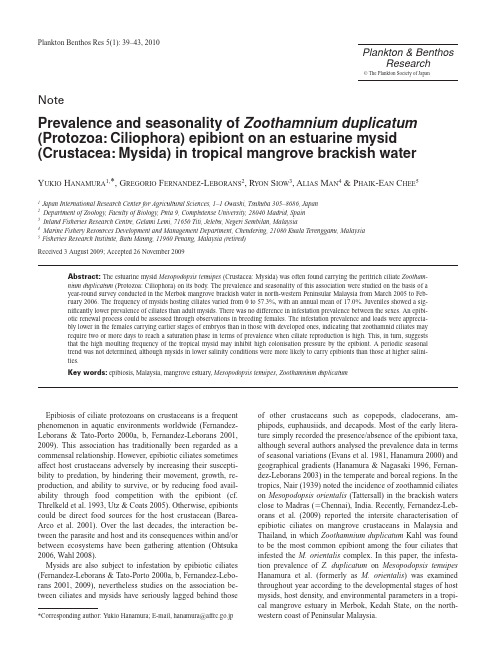
NoteMysids were sampled monthly at the morning low tide using a hand net (30cm mouth width, 0.77mm mesh width) in the intertidal zone at two sampling sites in the Merbok mangrove estuary (Stns. B and C: 5º 38ЈN, 100º 24ЈE), Peninsular Malaysia (Hanamura et al. 2008b), from March 2005 to Febru-ary 2006. All samples were ﬁxed immediately in approxi-mately 5% formalin seawater and preserved prior to subse-quent analyses. The sampling details, mysid density, and envi-ronmental conditions have been documented elsewhere (Hana-mura et al. 2008b; as M. orientalis ): for the taxonomic identity of the M. orientalis complex, see Hanamura et al. (2008a).Approximately 100 mysids, whenever possible, were ran-domly extracted from each sample and categorised according to the sexual developmental stages (Hanamura et al. 2008b). A total of 2,240 individuals of mysids were examined in this study. Infestation prevalence, deﬁned as the percentage of mysids with attached zoothamnid ciliates, was calculated using a stereomicroscope, and the samples were stained with methyl-ene blue when necessary. The epibiont load was also calcu-lated as the number of zooids on the host (no. of zooids host Ϫ1). Data from the two study sites were combined.In addition to seasonal analyses, 360 breeding females from selected collections (May, October, and November 2005),which were selected due to the highest zoothamnid ciliate inci-dence, were examined in order to evaluate the colonisation re-newal process more precisely. The breeding females were cate-gorised according to the degree of development of embryos carried in their brood pouches, and were denoted as F I (eggs/embryos corresponding to Fig. 19 in Nair (1939), later on), F IIa (Figs..20–21) and F IIb (Figs. 22–24), and F III (Fig. 25).In statistical analyses, differences were considered signiﬁcant at p Ͻ0.05.The colonial ciliate Z . duplicatum was frequently found in-festing the posterior part of the mysid body (posteroventral part of the sixth abdominal somite and base of the uropod close to the anus) (Fig. 1), but also occasionally was attached to the pleopods, or rostral plate, or the eye stalks (see also Fer-nandez-Leborans et al. 2009).This zoothamnid-mysid association was found almost as a year-round phenomenon at the study site, although the infesta-tion prevalence of Z. duplicatum on M. tenuipes showed a wide range of variation from 0 to 57.3%, with an annual mean of 17.0%. The infestation prevalence reached its maximum in December 2005, followed by May and September–November 2005, while no colonisation of ciliates was observed in the June–July samples, and the colonisation remained at very low levels in March and August 2005 (Fig. 2a). The overall infesta-tion prevalence of ciliates on mysids did not show any seasonal trend (run-test, r ϭ5, p Ͼ0.05; Tate & Clelland (1957)). Adult mysids exhibited two peaks of prevalence in May and Decem-ber of 2005, and relatively higher incidences were observed from September 2005 to February 2006 (Fig. 2a). In immature mysids, the highest prevalence of zoothamnid ciliates was ob-served in the December 2005 sample, followed by those in Oc-tober and September 2005. As compared with adults, juvenile mysids exhibited a smaller infestation peak in September40Y . H ANAMURA et al.Fig.1.Estuarine mysid Mesopodopsis tenuipes hosting a large colony of the peritrich ciliate Z oothamnium duplicatum (encir-cled): abdVI, sixth abdominal somite; tel, telson; urp, uropod.Fig.2.Seasonal changes in infestation prevalence (%) for Zoothamnium duplicatum epibiosis on mysids in the Merbok man-grove estuary according to developmental stages (a) and sexes (b)of Mesopodopsis tenuipes , and changes in salinity and host mysid’s abundance (c).2005. The infestation prevalence was signiﬁcantly different be-tween the developmental stages of mysids (Kruskal-Wallis test, 7.21, pϽ0.05), and juveniles were the least vulnerable group when compared to adults (Scheffe test, 7.21, pϽ0.05). There was no difference in infestation prevalence between the sexes (Fig. 2b) (Kruskal-Wallis test, 0.05, pϾ0.05). Epibiont loads on mysids were relatively low, and heavily infested mysids (Ͼ20 zooids hostϪ1) accounted for only 3.4% of the total mysids observed in the seasonal analyses. The infestation prevalence of zoothamnid ciliates in M. tenuipes in the Mer-bok mangrove estuary (17.0% in annual mean) was much lower when compared to Ͼ90% prevalence of peritrich ciliates attached to Archaeomysis articulata Hanamura in Ishikari Bay, northern Japan, in which the epibiont loads were also higher (often Ͼ50 zooids hostϪ1 ) (Hanamura 2000). In Lake Michi-gan, more than half of the population of Mysis diluviana Au-dzijonte & Väinölä (as M. relicta) were heavily infested (Ͼ20 zooids) by a suctorian ciliate, Tokophrya sp. (Evans et al. 1981). Furthermore, Fernandez-Leborans (2003) found that the number of peritrich ciliates V orticella sp. attached to the Lake Lüsˇiai mysids was 390 (mean).Amongst the heavily infested mysids, larger females carried more zoothamnid ciliates and decreasing frequency was as fol-lows (total Nϭ76): breeding females (52.6% in prevalence), adult males (21.1%), adult females (13.2%), immature females (6.6%), juveniles (3.9%), and immature males (2.6%). In the breeding females caught during the periods when ciliate inci-dence was high, heavily infested females were found only among those with developed embryos (Nϭ29); FIII(16.5%),F IIb (12.8%), FIIa(0%), and FI(0%). Similar results have oftenbeen reported for other ciliate-crustacean associations (Xu 1992, Hanamura 2000, Fernandez-Leborans 2003), while some other studies have indicated host-size independence (Evans et al.1981). Also, an inverse relationship between infestation in-tensity and size/age of host has even been reported (Utz & Coats 2005). Warm water species/population of mysids have shorter inter-moult periods than those in colder water habitats (Mauchline 1980), and this could be a factor hampering more intensive colonisation pressure from epibionts (Threlkeld et al. 1993). Indeed, the infestation prevalence could exceed 80% in breeding females (see discussion below), which may have the longest instar duration of the mysid population.Water salinity had a broad range from 16.70 to 30.83 (an-nual mean 25.13Ϯ4.93) depending on the survey (Fig. 2c) (see also H anamura et al. 2008b). Despite the fact that a Kendall rank correlation test failed to ﬁnd a signiﬁcant relationship (Fig. 3a), there was a weak correlation between the incidence of zoothamnid ciliates and salinity, as infestation levels be-come higher with decreasing salinity (rϭϪ0.62, pϽ0.05), and salinity is likely to be correlated to the population dynamics of Z. duplicatum. López et al. (1998) found that, in a freshwater reservoir in western Venezuela, the incidence of epibionts dominated by Epystylis species increased in close correspon-dence to the rainy season. However, it remains unclear whether the increase in prevalence was the result of low salinity or is due to other factors. Salinity changes in the studied estuary occur basically as a consequence of rainfall and could con-tribute to possible increasing the inﬂow of organic matter from the surrounding land, which is essential for the ciliates. Eu-trophication in the aquatic environment is undoubtedly one of the major factors in enhancing the colonisation of epibiotic cil-iates (Henebry & Ridgeway 1979, Xu 1992). The water tem-perature remained constant at around 30°C (annual mean 30.1°CϮ1.12) throughout the year except for December 2006, when an unusually low value of 27°C was recorded; hence, water temperature is not a strong factor contributing to the epibiotic ﬂuctuations observed in this study. The epibiotic sys-tem, however, may be regulated by complex interactions be-tween the epibiont and host or between biological and environ-mental parameters or by a combination of both bio- and abiotic factors (Utz & Coats 2005).Higher infestation prevalence and also load have occasion-ally been observed when the host species were more abundant, but also many neutral or negative observations have been recorded (cf. Threlkeld et al. 1993, Utz & Coats 2005). The density of mysids at the study site showed a broad range of ﬂuctuations from 12 to 2,273indiv.mϪ2(annual mean 709indiv. mϪ2) (Fig. 2c).The infestation prevalence was irrele-vant to the catch abundance of host mysids (rϭ0.26, pϾ0.05) (Fig. 3b). Epibiotic ciliates including Z. duplicatum at the stud-ied site were able to utilise a variety of crustacean substrates (Fernandez-Leborans et al. 2009) included M. tenuipes, which was not the sole host for the ciliates.The females in the early breeding phases (FIand FIIa) showed a signiﬁcantly lower incidence of ciliates than those inthe later ones (FIIband FIII) (c2test, 78.34, pϽ0.05); the pro-portion of mysids with ciliates attached (and also epibiont loads) intensiﬁed in the late phases of breeding females, reach-ing well beyond 80% (Fig. 4). The life cycle of sessile peritrich ciliates is generally comprised of a stalked, sessile feeding stage (trophont) and a free-swimming dispersal stage (telotroch), although the mechanism inducing these phases is not well-known. Zoothamnium duplicatum settled less readily on the new exoskeleton of mysids, and its attachment appearedto be intensiﬁed after the FIIaphase of breeding mysids. A sim-ilar pattern, slow at ﬁrst and exponential later, was observed by Xu (1992) in a ciliate-cladoceran association in nature.The development of mysid embryos progresses in a mater-nal brood pouch, while females do not moult during the breed-ing process (Mauchline 1980). This makes the embryos, such as the parthenogenic eggs of cladocerans (Threlkeld et al. 1993), useful as a chronological indicator. An examination of epibiosis in egg-bearing females, therefore, can be advanta-geous to assess how the colonisation of ciliates proceeds from the time of their last ecdysiast, which takes place shortly be-fore egg production. Nair (1939) found that egg extrusion of M. orientalis, the closest relative of M. tenuipes, takes place at night, and these eggs (or embryonic larvae) subsequently spend about 96 h (4 days) in the brood pouch at a water tem-perature of 24–29°C, where the ﬁrst moult (Egg stageI IIa) occurs after about 24 h. If this time duration is applicable to M. tenuipes, the Z. duplicatum population would require at leastZoothamnid epibiosis in estuarine mysid41two days to achieve a stationary phase of settlement, although the epibiont loads may continue to increase gradually with the age of the mysid (the duration of the instars). The egg size of M. tenuipes is slightly larger than that of M. orientalis (0.42mm in mean vs. 0.37mm) (Hanamura et al. 2008b), al-though the incubation time for the embryos of M. tenuipes in the studied estuary is assumed to be not very different from that of M. orientalis in terms of egg size and water tempera-ture, which signiﬁcantly inﬂuence the incubation time of em-bryos (Wittmann 1984).There was an absence of zoothamnid ciliates on the sergestid shrimp Acetes japonicus Kishinouye sampled in a marine habitat (Fernandez-Leborans et al. 2009, H anamura pers. obser.). Similarly, we did not detect any incidence of M. orientalis carrying Z. duplicatum despite conducting a year-round survey off the southern coast of Penang Island, Malaysia (H anamura pers. obser.). In contrast, another species of sergestid shrimp Acetes sibogae Hansen and/or juvenile of the banana shrimp Fenneropenaeus merguiensis(De Man), both of which were typical residents of the inner mangrove swamp, were regarded as preferential substrates for the ciliates (Fer-nandez-Leborans et al. 2009). These ﬁndings suggest that this type of interaction, between Z. duplicatum and planktonic crustaceans, could be uncommon in marine coastal habitats. The presence of zoothamnid ciliates may be a useful bio-indi-cator for discriminating a crustacean population with a closer afﬁnity to a mangrove estuary than a coastal habitat.AcknowledgementsWe appreciate and give thanks to Mr. Faizul Mohd Kassim for his invaluable assistance in the ﬁeld and the laboratory and to Messrs Ismail bin Awang Kechik and Raja Mohammad No-ordin bin Raja Omar Ainuddin, former and present directors of the Fisheries Research Institute, Penang, for providing neces-sary facilities for this study. We also thank Drs. Noriyuki Koizumi and Shinsuke Morioka for their technical support. Comments from the reviewers are also acknowledged. This study was supported in part by a research grant from the Japan Society for the Promotion of Science (20570101).ReferencesBarea-Arco J, Pérez-Martínez C, Morales-Baquero R (2001) Evidence of a mutualistic relationship between an algal epibiont and its host, Daphnia pulicaria. Limnol Oceanogr 46: 871–881.Evans MS, Sell DW, Beeton AM (1981) Tokophrya quadripartita and Tokophrya sp. (Suctoria) associations with crustacean zooplankton in the Great Lakes region. Trans Am Microsc Soc 100: 384–391. Fernandez-Leborans G (2001) A review of the species of protozoan epibionts on crustaceans. III. Chonotrich ciliates. Crustac Int J Crustac Res 74: 581–607.Fernandez-Leborans G (2003) Comparative distribution of protozoan epibionts on Mysis relicta Lovén, 1869 (Mysidacea) from three lakes in northern Europe. Crustac Int J Crustac Res 76: 1037–1054. Fernandez-Leborans G (2009) A review of recently described epibioses of ciliate Protozoa on Crustacea. Crustac Int J Crustac Res 82: 167–189. Fernandez-Leborans G, H anamura Y, Siow R, Chee P-E (2009) Intersite epibiosis characterization on dominant mangrove crustacean species from Malaysia. Contrib Zool 78: 9–23.Fernandez-Leborans G, Tato-Porto ML (2000a) A review of the species of42Y. H ANAMURA et al.Fig.3.Relationships between the infestation prevalence and salinity (a) and between the infestation prevalence and mysid abundance (b).Fig.4.Infestation prevalence in female Mesopodopsis tenuipes carrying embryos of each developmental stage. Numbers in paren-theses indicate individual numbers of mysids examined.protozoan epibionts on crustaceans. I. Peritrich ciliates. Crustac Int J Crustac Res 73: 643–683.Fernandez-Leborans G, Tato-Porto ML (2000b) A review of the species of protozoan epibionts on crustaceans. II. Suctorian ciliates. Crustac Int J Crustac Res 73: 1205–1237.Hanamura Y (2000) Seasonality and infestation pattern of epibiosis in the beach mysid Archaeomysis articulata. Hydrobiologia 427: 121–127.H anamura Y, Koizumi N, Sawamoto S, Siow R, Chee P-E (2008a) Re-assessment of the taxonomy of the shallow-water Indo-Australasian mysid Mesopodopsis orientalis(Tattersall, 1908) and proposal of a new species with an appendix on M. zeylanica Nouvel, 1954. J Nat Hist 42: 2461–2500.H anamura Y, Nagasaki K (1996) Occurrence of the sandy beach mysids Archaeomysis spp. (Mysidacea) infested by epibiontic peritrich ciliates (Protozoa). Crustac Res 25: 25–33.Hanamura Y, Siow R, Chee P-E (2008b) Reproductive biology and season-ality of Mesopodopsis orientalis(Tattersall, 1908) (Crustacea: Mysi-dacea) in a tropical mangrove estuary, Malaysia. Est Coast Shelf Sci 77: 467–474.Henebry MS, Ridgeway BT (1979) Epizoic ciliated Protozoa of planktonic copepods and cladocerans and their possible use as indicators of organic water pollution. Trans Am Microsc Soc 98: 498–508.López C, Ochoa E, Páez R, Theis S (1998) Epizoans on a tropical fresh-water crustacean assemblage. Mar Freshw Res 49: 271–276.Mauchline J (1980) The biology of mysids and euphausiids. Adv Mar Biol 18: 1–677.Nair KB (1939) The reproduction, oogenesis and development of Mesopodopsis orientalis Tatt. Proc Indian Acad Sci 9: 175–223. Ohtsuka S (2006) Importance of parasito-planktology for precise under-standing the marine ecosystem. Bull Plankton Soc Japan 53: 7–13. (in Japanese)Tate MW, Clelland RC (1957) Nonparametric and Shortcut Statistics in the Social, Biological, and Medical Sciences. Interstate Prints & Publishing, Inc., Illinois, 171 pp.Threlkeld ST, Chiavelli DA, Willey RL (1993) The organization of zoo-plankton epibiont communities. Trends Ecol Evol 8: 317–321.Utz LRP, Coats W (2005) Spatial and temporal patterns in the occurrence of peritrich ciliates as epibionts on calanoid copepods in the Chesapeake Bay, USA. J Eukaryot Microbiol 52: 236–244.Wahl M (2008) Ecological lever and interface ecology: epibiosis modu-lates the interactions between host and environment. Biofouling 24: 427–438.Wittmann KJ (1984) Ecophysiology of marsupial development and repro-duction in Mysidacea (Crustacea). Oceanogr Mar Biol Annu Rev 22: 393–428.Xu Z (1992). The abundance of epizoic ciliate Epistylis daphniae related to their host Moina macrocopa in an urban stream. J Invertebr Pathol 60: 197–200.Zoothamnid epibiosis in estuarine mysid43。

《2024年基于肠-脑轴理论探讨甘松对帕金森大鼠运动功能障碍的改善作用及机制》范文

《基于肠-脑轴理论探讨甘松对帕金森大鼠运动功能障碍的改善作用及机制》篇一一、引言帕金森病（PD）是一种常见的神经系统退行性疾病，主要表现为运动功能障碍，包括静止性震颤、运动迟缓、肌强直和姿势平衡障碍等。

尽管目前对帕金森病的治疗方法多样，但仍然缺乏有效的根治手段。

近年来，随着肠-脑轴理论的深入研究，越来越多的研究表明肠道微生物与中枢神经系统疾病之间存在密切的联系。

甘松作为一种传统中药，具有广泛的药理作用。

本文基于肠-脑轴理论，探讨甘松对帕金森大鼠运动功能障碍的改善作用及机制。

二、材料与方法1. 实验材料本实验选用成年SD大鼠，建立帕金森病模型。

甘松药材购自正规药材市场，经鉴定后使用。

实验所需试剂及仪器均符合实验要求。

2. 方法（1）建立帕金森大鼠模型：采用6-羟基多巴胺（6-OHDA）注射法建立PD大鼠模型。

（2）分组与给药：将大鼠随机分为模型组、甘松治疗组和对照组，分别进行不同剂量的甘松灌胃治疗。

（3）行为学检测：观察并记录各组大鼠的运动功能变化。

（4）肠-脑轴相关指标检测：检测肠道微生物、肠道炎症因子、脑内神经递质等指标。

（5）统计学分析：采用SPSS软件进行数据分析，比较各组之间的差异。

三、结果1. 甘松对帕金森大鼠运动功能的改善作用实验结果显示，经过甘松治疗后的帕金森大鼠，其运动功能得到显著改善，静止性震颤、运动迟缓等症状有所减轻。

行为学检测结果表明，甘松治疗组的大鼠运动能力较模型组有明显提高。

2. 甘松对肠-脑轴相关指标的影响（1）肠道微生物：甘松治疗能够调节帕金森大鼠肠道微生物的组成，增加有益菌群的数量，降低有害菌群的比例。

（2）肠道炎症因子：甘松能够降低帕金森大鼠肠道炎症反应，减少炎症因子的释放。

（3）脑内神经递质：甘松能够提高脑内多巴胺等神经递质的含量，从而改善帕金森大鼠的运动功能。

四、讨论本实验结果表明，甘松能够改善帕金森大鼠的运动功能障碍，其作用机制可能与调节肠-脑轴相关。

甘松通过调节肠道微生物的组成，降低肠道炎症反应，进而影响脑内神经递质的含量，从而改善帕金森大鼠的运动功能。

原生动物季节性群落结构研究

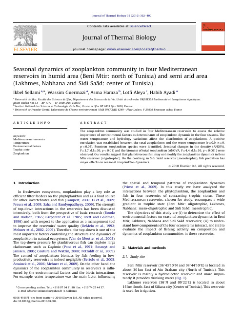
Seasonal dynamics of zooplankton community in four Mediterranean reservoirs in humid area (Beni Mtir:north of Tunisia)and semi arid area(Lakhmes,Nabhana and Sidi Sa ˆad:center of Tunisia)Ikbel Sellami a ,n ,Wassim Guermazi a ,Asma Hamza b ,LotﬁAleya c ,Habib Ayadi aaUniversite´de Sfax,Faculte ´des Sciences de Sfax,De ´partement des Sciences de la Vie.Unite ´de recherche UR/05ES05Biodiversite ´et Ecosyst e mes Aquatiques.Route soukra Km 3.5–BP 1171–CP 3000Sfax,Tunisie bInstitut National des Sciences et Technologie de la Mer,Centre de Sfax BP 1035Sfax 3018,Tunisie cUniversite ´de Franche-Comte ´,Laboratoire de Chrono-environnement,UMR UFC/CNRS 6249—Place Leclerc,F-25030Besanc -on cedex,Francea r t i c l e i n f o Keywords:Mediterranean reservoirs TemperatureEnvironmental factors Trophic state Zooplanktona b s t r a c tThe zooplankton community was studied in four Mediterranean reservoirs to assess the relativeimportance of environmental factors as determinants of zooplankton dynamic in the four seasons.The water temperature and hydrology variations affect the distribution of zooplankton.A positive correlation was established between the total zooplankton and the water temperature (r ¼0.9,n ¼9,p o 0.05).Fourteen zooplankton species were identiﬁed.Seasonal changes in the density (ANOVA,F ¼3.7,d.f ¼36,p o 0.01)and the biomass of total zooplankton (ANOVA,F ¼4.4,d.f ¼36,p o 0.001)were observed.Our results suggest that planktivorous ﬁsh may not modify the zooplankton dynamics in Beni Mtir reservoir (oligotrophic).On the contrary,in Sidi Saˆa d reservoir (mesotrophic),ﬁsh predation has major effects on seasonal zooplankton dynamics.&2010Elsevier Ltd.All rights reserved.1.IntroductionIn freshwater ecosystems,zooplankton play a key role as efﬁcient ﬁlter feeders on the phytoplankton and as a food source for other invertebrates and ﬁsh (Lampert,2006;Li et al.,2009;Preuss et al.,2009;Saha and Bandyopadhyay,2009).The strength of top-down interactions in the reservoirs has been discussed intensively,both from the perspective of basic research (Brooks and Dodson,1965;Carpenter et al.,1985;Brett and Goldman,1996)and with respect to the application as a management tool to improve the reservoirs’water quality (DeMelo et al.,1992;Mehner et al.,2002,2009).Therefore,the top-down is one of the most important factors controlling the structure and dynamics of zooplankton in natural ecosystems (Van de Meutter et al.,2005).The top-down pressure by planktivorous ﬁsh can deplete large cladocerans such as Daphnia (Pont et al.,1991;Bossuyt and Janssen,2005;Couture and Watzin,2008;Petzoldt et al.,2009).The control of zooplankton biomass by ﬁsh feeding in low-productivity reservoirs is indeed negligible (Bertolo et al.,2005;Amsinck et al.,2006;Mehner et al.,2009).On the other hand,the dynamics of the zooplankton community in reservoirs is inﬂu-enced by the environmental factors and the biotic interactions.For example,water temperature was the main factor inﬂuencingthe spatial and temporal patterns of zooplankton dynamics (Primo et al.,2009).In this study we have analyzed the interactions between the phytoplankton,the zooplankton and ﬁsh in four reservoirs of contrasting trophic status.These Mediterranean reservoirs,chosen for study,encompass a wide gradient in trophic state (Beni Mtir:oligotrophic,Lakhmes,Nabhana:meso-oligotrophic and Sidi Saˆa d:mesotrophic).The objectives of this study are (i)to determine the effect of environmental factors on seasonal zooplankton dynamics in Beni Mtir,Lakhmes,Nabhana and Sidi Saˆa d reservoirs;(ii)to under-stand how components of the four ecosystems interact,and (iii)to evaluate the impact of ﬁshing activity on composition and dynamics of zooplankton communities in these reservoirs.2.Materials and methods 2.1.Study siteBeni Mtir reservoir (3614301000N and 0814401000E)is located in about 30km East of Ain Draham city (North of Tunisia).This reservoir is mainly a hydroelectric reservoir and more impor-tantly it provides drinking water (Fig.1).Lakhmes reservoir (361N and 091220E)is located in about 15km South-East of Siliana city (Center of Tunisia).This reservoir is used for irrigation.Contents lists available at ScienceDirectjournal homepage:/locate/jtherbioJournal of Thermal Biology0306-4565/$-see front matter &2010Elsevier Ltd.All rights reserved.doi:10.1016/j.jtherbio.2010.08.004nCorresponding author.Tel.:+21697642180;fax:+21674274437.E-mail address:sellamifss@yahoo.fr (I.Sellami).Journal of Thermal Biology 35(2010)392–400Nabhana (361030N and 091540E)and Sidi Saˆa d reservoirs(3513104000N and 0915903000E)are situated about 50and 30kilometers South of Kairouan city,respectively (Center of Tunisia).These two reservoirs were constructed to protect the city of Kairouan against the violent ﬂoods of the river and also to irrigate the agricultural land.Morphometric and other basic characteristic of these Mediterranean reservoirs are shown in Table 1.2.2.Environmental factorsThe samples were collected in spring (March–May),summer (June–July–August),autumn (September–October)and winter (December–January;2005–2006)in the deepest central area of the studied reservoirs.At this station,a depth-integrated sample was taken by pooling samples from surface,5and 10m deep,to represent the entire water column.Water samples for physico-chemical analyses were collected using a 1l Van Dorn bottle at the same depth and preserved in cold and dark conditions.The water temperature (1C),pH,dissolved oxygen and water transparency were measured in situ.Water temperature,dissolved oxygen concentration (mg l À1)and pH were measured using a multiparameter probe (Multi 340i/SET).The concentration of the suspended matter (mg l À1)was determined by measuring the dry weight of the residue after ﬁltration through a Whatman GF/C membrane.Nutrient concentra-tions were analyzed by standard colorimetric techniques with an automatic Bran and Luebbe type 3analyzer and were expressed as mg l À1.Air temperature,evaporation and precipitation were obtained from the meteorology service of Tunisia.1/20.000(2)1/20000(1)(3)1/20000(4)1/20000NFig.1.Location of the studied reservoirs 1:Beni Mtir,2:Lakhmes,3:Nabhana and 4:Sidi Saˆa d.Table 1Morphometric and hydrologic characteristics of the studied reservoirs.Beni MtirLakhmesNabhanaSidi Sa ˆad Location Longitude 3614301000N,361N,361030N,3513104000N,Latitude0814401000E 091220E 091540E 0915903000E Construction (year)1953196619661981Area (ha)310.61025321800Catchment area (Km 2)1031318558650Volume (106m 3)57.61486209Annual mean air temperature (1C)16.718.120.122.4Annual mean evaporation (mm)90.2129.8147.2145.1Annual mean precipitation (mm)123.346.928.827.2I.Sellami et al./Journal of Thermal Biology 35(2010)392–400393Phytoplankton samples were taken using a1l Van Dorn bottle, simultaneously with the samples for chemical analysis.Phyto-plankton enumeration was performed with an inverted micro-scope using the Uterm¨ohl(1958)method afterﬁxation with a Lugol solution.Sub samples(0.5l)for quantiﬁcation of chlorophyll a,were ﬁltered using Whatman GF/Cﬁlters(1.2m m pore sizeﬁlter and 25mm-diameter)and pigment extraction was performed with 90%acetone(Lorenzen,1967).The concentrations were deter-mined by the spectrophotometry based on the absorbance at750 and663nm.Fish density was obtained from the ministry of agriculture of Tunisia.2.3.ZooplanktonZooplankton samples were taken using a55m m mesh Juday plankton net(25cm in diameter)and preserved with4%formalin and stained with Bengal Pink.The zooplankton was enumerated and counted under a binocular microscope type leica in Dolffus chambers(Paterson,1993).The taxonomic identiﬁcation was carried out according to Dussart(1969),Koste(1978),Stella (1982),Margaritora(1985),Pourriot and Francez(1986),Kor-ovchinsky(1992).Zooplankton was presented in terms of abundance(ind lÀ1)and biomass(m g lÀ1).For biomass estima-tions of cladocerans and copepods,100individuals(whenever possible)per genus and/or species from each reservoir were measured and biomass was calculated according to Bottrell et al. (1976).The level of community structure was assessed according to the diversity index(H0)and Simpson index(D)are described by Shannon and Weaver(1949)and Steel et al.(1997),respectively. These indexes were calculated from the annual average density of zooplanktonic species:H u¼ÀX Si¼1n iNÂlog2n iNwhere n i is the average density of i species,and N is the average density of the entire community,respectively.1ÀD¼1-SðN iÂNÀ1Þ2N i is the density of i species,N is the number of species.2.4.Statistical analysisThe data recorded in this study for each taxon(abundance or biomass)and physicochemical variables were log(x+1) transformed because of signiﬁcant deviation from normal dis-tribution.The data were examined with a normalized principal component analysis(PCA)(Chessel and Doledec,1992).Pearson’s product–moment correlation coefﬁcient r was calculated to determine the association between the physicochemical variables and the zooplankton community(Zar,1999).Additionally,an independent one-way ANOVA and Tukey’s test were run to assess the effect of the temporal variation on zooplankton density and biomass.It was also used to compare physicochemical variables between all the reservoirs and between the seasons.3.Results3.1.Environmental parametersWater temperature was low in the spring-winter seasons (8.470.5and8.470.91C recorded in winter)and high in the summer–autumn seasons(22.271.8and26.370.71C recorded in summer)in Beni Mtir and Sidi Saˆa d.However,in Lakhmes and Nabhana the highest temperature was recorded in spring–summer–autumn(25.770.7and26.470.31C recorded in summer)(Table2).A signiﬁcant variation of water temperature was observed between the reservoirs(ANOVA,F¼39.6, d.f¼33,p o0.001).Dissolved oxygen concentrations were relatively constant in Nabhana reservoir. The highest values averaging7.970.3mg lÀ1in winter and 7.870.5mg lÀ1in spring were found in Sidi Saˆa d and Beni Mtir, respectively.Differences of dissolved oxygen concentrations between the reservoirs were established(ANOVA,F¼25.5,d.f¼33,p o0.001). The pH valuesﬂuctuated from6.570.01in spring to9.470.4in winter in Nabhana and Beni Mtir respectively.Suspended matter concentrations reached the highest values in winter in Lakhmes, Nabhana and Sidi Saˆa d;which is explained by the adjacent soil leaching promoted by rain.Variations of suspended matter concen-trations were observed between the reservoirs(ANOVA,F¼7.3, d.f¼33,p o0.05).Nutrients concentrations(NH4+,T-N,PO43Àand T-P) did not differ signiﬁcantly between the reservoirs(Table2).The chlorophyll a concentrations varied from2.171.1m g lÀ1in spring to11.174.6in winter in Beni Mtir and Sidi Saˆa d reservoirs. The difference in the chlorophyll a concentrations between the reservoirs sampled was negligible(ANOVA,F¼4.2,d.f¼33,p o0.05).3.2.Seasonal dynamics of zooplanktonA total of four copepods species(Copidodiaptomus numidicus, Acanthocyclops robustus,Acanthocyclops viridis,Cyclops strenuus), four cladocerans(Bosmina longirostris,Ceriodaphnia quadrangula, Diaphanosoma brachyurum,Daphnia longispina)and six rotifers (Asplanchna sp.,Filinia longiseta,Hexarthra mira,Keratella quad-rata,Keratella cochlearis,Brachionus urceolaris)were found in the studied reservoirs(Table3).The highest zooplankton densities were found in Lakhmes (49.5755.5ind lÀ1)and Nabhana(28.0723.7ind lÀ1)and the lowest in Beni Mtir(16.6720.8ind lÀ1)and Sidi Saˆa d (13.3717.5ind lÀ1)reservoirs.The peak of density(216.5ind lÀ1)(Fig.2a)and biomass(1.2Â103m g lÀ1)(Fig.2b)were observed in autumn in Lakhmes reservoir.Seasonal changes in the density(ANOVA,F¼3.7, d.f¼36,p o0.01)and biomass of zooplanktonic organisms(ANOVA,F¼4.4, d.f¼36,p o0.001) revealed signiﬁcant differences between reservoirs.Theﬁsh predation pressure signiﬁcantly inﬂuenced the abundance of zooplankton especially in Sidi Saˆa d reservoir (Fig.2c).This was indicated by the signiﬁcant negative correla-tions betweenﬁsh and zooplankton abundance(r¼À0.9,n¼9, p o0.05).C.numidicus was the dominant species in Lakhmes,Nabhana and Beni Mtir with densities averaging63.3772.1,36.8734.3 and22.6723.8ind lÀ1,respectively(Table3).This species presented its maximum abundance(236.7ind lÀ1)in autumn at a depth of5m in Lakhmes reservoir(Fig.3a).However,A.viridis was the most abundant in Sidi Saˆa d reservoir(13.1718.8ind lÀ1). This species was positively correlated with chlorophyll a concentrations(r¼0.9,p o0.05).C.strenuus was found only in Beni Mtir with maximum in spring at a depth of10m(1.7ind lÀ1) (Fig.3c)and A.viridis and B.urceolaris in Sidi Saˆa d reservoir in summer at a depth of10m(52.2ind lÀ1)and5m(1.7ind lÀ1), respectively(Fig.3d).D.brachyurum,H.mira and K.quadrata were the most common species found in all reservoirs.The highest taxa richness was found in Lakhmes and Nabhana with11and10species,respectively.A higher community diversiﬁcation was noticed in summer and autumn(H0¼1.8bits ind lÀ1,D¼0.6)in Lakhmes reservoir.Whereas,Sidi Saˆa d reservoir exhibited the lowest richness(6species).I.Sellami et al./Journal of Thermal Biology35(2010)392–400 394munity analysisTheﬁrst two PCA axes explain as a whole82.18%of the total variance(Fig.4).Theﬁrst axis explains53.75%of the total variance separates Lakhmes and Nabhana reservoirs,which present a high density and biomass of zooplankton and considerable richness in B.longirostris,K.quadrata,K.cochlearis and Asplanchna sp.from Sidi saˆa d reservoir with A.robustus, A.viridis, B.urceolaris and D.brachyurum.The second axis explaining28.42%of the total variance is associate with Beni Mtir reservoir(heavy precipitation), with the species C.strenuus and D.longispina.The most discriminant physicochemical variables,Chl a,NH4+, and T-P were strongly associated with axis1and axis2, respectively,indicating that these two axes were mainly related to trophic status.Along the gradient of trophic status,rotifer species were found at high trophic status.Table2Environmental parameters(mean7SD,standard deviation)in the four reservoirs studied(S:spring;Sm:summer;A:autumn;W:winter).Beni Mtir LakhmesS Sm A W S Sm A WT(1C)13.670.3a22.271.8a21.272.3a8.470.5a24.970.1b25.770.7b20.470.8b8.670.6bO2(mg lÀ1)7.870.5a 5.270.1a 3.170.3a 2.671.1a 5.370.3b 4.870.3b 2.170.02b 2.570.4b pH8.070.04a8.370.04a8.970.4a9.470.4a8.270.18.370.038.070.27.970.4 MES(mg lÀ1)59.2716.736.471.542.779.248.1722.416.772.4b27.671.9b24.573.3b84.3714.7b NOÀ2(mg lÀ1)0.0570.01a0.0470.02a0.0370.01a0.0870.01a0.0970.010.0870.010.0870.010.0870.06 NOÀ3(mg lÀ1)0.2870.05a0.1170.04a0.1870.04a0.0570.04a0.3170.01b0.2370.01b0.3570.03b0.0670.02b NHþ4(mg lÀ1)0.0370.010.0470.020.0370.020.0570.040.0570.050.0670.020.1070.030.0570.05T-N(mg lÀ1)0.2670.060.2570.030.4370.110.2670.110.4870.050.3270.040.4770.02 1.0470.87 PO3À4(mg lÀ1)0.0770.010.0470.010.067.010.0670.020.0370.010.0370.010.0770.070.0570.01T-P(mg lÀ1)0.0570.010.0670.010.0770.020.0570.010.0470.01b0.0570.01b0.0670.02b0.0370.01b Chl a(m g lÀ1) 2.171.1a7.370.5a 5.171.3a 2.870.8a 3.370.2 5.070.4 4.171.1 4.872.3Nabhana Sidi Saˆa d F(d.f)S Sm A W S Sm A WT(1C)22.270.7c26.470.3c21.870.2c9.770.1c15.570.8d26.370.7d25.672.2d8.470.9d39.6(11)nnn O2(mg lÀ1) 4.670.03c 5.570.1c 4.270.6c 3.570.5c 6.270.6d 4.470.7d 3.770.1d7.970.3d25.5(11)nnn pH 6.570.01c8.470.03c8.470.04c8.470.1c8.570.18.270.18.270.18.470.134.2(11)nnn MES(mg lÀ1)17.372.8c27.270.9c19.771.6c78.0735.7c19.173.1d24.575.7d24.371.8d33.473.1d7.3(11)nNOÀ2(mg lÀ1)0.0970.01c0.0270.01c0.0370.01c0.0470.01c0.0270.01d0.0170.01d0.0470.01d0.0270.01d25.7(11)nnnNOÀ3(mg lÀ1)0.2970.01c0.1370.02c01870.04c0.1370.04c0.2370.05d0.0770.02d0.2270.01d0.0470.01d28.6(11)nnn NHþ4(mg lÀ1)0.0570.050.0470.010.0670.020.0570.050.0470.01d0.0270.01d0.0670.02d0.0370.01d 2.4(11)T-N(mg lÀ1)0.4470.05c0.2970.01c0.4570.08c0.2770.11c0.2570.01d0.3370.05d0.2970.01d 1.5771.08d 2.0(11)PO3À4(mg lÀ1)0.0470.01c0.0270.01c0.0670.02c0.0670.01c0.0270.010.0570.020.0370.010.1470.11 1.1(11)T-P(mg lÀ1)0.0470.010.0770.010.0770.020.0770.010.0670.010.0570.10.0470.010.0770.02 3.8(11)Chl a(m g lÀ1) 3.470.3c 6.971.2c 5.970.5c 4.371.4c 4.570.8 4.072.67.774.311.174.6 4.2(11)nF-value:between-groups mean square/within-groups mean square.Values in the same row showing the same letters are signiﬁcantly different as tested with one-way ANOVA coupled by Tukey test.nn p o0.01n p o0.05.nnn p o0.001.Table3Density(ind lÀ17standard deviation,SD)and biomass(m g lÀ17standard deviation,SD)of zooplankton species in the four reservoirs.Beni Mtir Lakhmes Nabhana Sidi Saˆa dDensity Biomass Density Biomass Density Biomass Density Biomass CopepodaCopidodiaptomus numidicus22.6723.8159.87168.663.3772.1496.37565.436.8734.3232.97217.0Acanthocyclops robustus0.871.2 3.975.70.370.5 1.372.4 1.371.49.4710.2 Acanthocyclops viridis13.1718.843.4762.2 Cyclops strenuus0.370.4 2.073.2CladoceraBosmina longirostris 6.077.5 6.578.10.0870.10.170.1Ceriodaphnia quadrangula 5.077.439.8758.68.0712.418.7729.2 3.375.1 6.479.7Diaphanosoma brachyurum 1.573.1 3.978.17.8712.5 6.079.610.8713.013.1715.811.8720.519.5734.1 Daphnia longispina 3.175.665.17115.1 2.275.344.67106.1RotiferaAsplanchna sp.0.0170.030.0970.2 3.477.921.9750.9 4.176.933.8756.7Filinia longiseta0.571.8 1.073.3 6.679.211.9716.40.0270.070.0170.05Hexarthra mira0.0270.070.00770.020.00970.030.00170.0050.371.20.170.60.170.30.0370.1 Keratella quadrata0.00870.020.0170.060.671.0 1.672.80.0870.10.270.50.0770.10.1370.2 Keratella cochlearis0.0670.10.0970.10.0570.090.0670.1Brachionus urceolaris0.370.60.370.6I.Sellami et al./Journal of Thermal Biology35(2010)392–4003954.DiscussionThe present study has shown a clear pattern (in density,biomass and composition)of seasonal zooplankton ﬂuctuation in the four reservoirs of Beni Mtir,Lakhmes,Nabhana and Sidi Saˆa d.The maximal zooplankton levels have generally been detected during summer and autumn,in June (Nabhana),in July (Beni Mtir),in August (Sidi Saˆa d)and in September (Lakhmes).The highest densities of total zooplankton were observed in Lakhmes andNabhana.This is associated with the high temperature values which were observed in spring–summer–autumn (25.770.7and 26.470.31C recorded in summer;Table 2).Positive correlation was found between total zooplankton and temperature (r ¼0.9,n ¼9,p o 0.05).The lowest abundance of total zooplankton was observed in winter in all reservoirs (Lakhmes:48.5ind l À1;Nabhana:36.9ind l À1;Sidi Saˆa d:7.3ind l À1;Beni Mtir:1.5ind l À1;D e n s i t y (i n d l -1) B i o m a s s (µg l -1)20406080100LakhmesNabhanaBeni MtirSidi SaâdSpringSummer Autumn Winter(%)0.00.20.40.60.81.01.21.4050100150200250Fig.2.Seasonal distribution of total zooplankton and zooplankton groups density (a)and Biomass (b)and abundance of ﬁsh (c)in the four reservoirs.I.Sellami et al./Journal of Thermal Biology 35(2010)392–400396Fig.2)during the period of low temperature ranging from 8.4to9.71C (Table 2).The same results were found by Lam-Hoai et al.(2006).Therefore,water temperature was a keystone element in the seasonal dynamics of zooplankton (Ortega-Mayagoitia et al.,2000;Zhou et al.,2001;Primo et al.,2009).This factor may indeed regulate most ecological mechanisms in temperate reservoirs (Ronnenberger et al.,1993).On the other hand,the lowest zooplankton density and biomass was related to heavy precipitation.Thus,a maximum value was found in Beni Mtir reservoir (123.3mm,Table 1).Many reports associate reduced zooplankton densities with important rainfall (Dejen et al.,2004;Guevara et al.,2009).Negative association was established between phytoplankton and zooplankton.This relation might have resulted from increased regulation of algal biomass by zooplankton grazing.100806040200(%)100806040200(%)S p r i n gS u m m e rA u t u m n W i n t e rFig.3.Seasonal distribution of zooplankton species in Lakhmes (a),Nabhana (b),Beni Mtir (c)and Sidi Saˆa d (d)reservoirs.I.Sellami et al./Journal of Thermal Biology 35(2010)392–400397Similar ﬁndings were obtained by many studies (Forrest and Arnott,2007;Williamson et al.,2007;Fragoso et al.,2008;Leoni and Garibaldi,2009;Lopes et al.,2009).It is well known that in natural lake ecosystems the biomass of zooplankton is likely to be determined by both phytoplankton (bottom-up effect)and zooplanktivores (top–down controls;Liu et al.,2007).Zooplanktivorous ﬁsh density has been associated with changes in zooplankton community density and composition (Hunt et al.,2003;Van De Bund et al.,2004;Korosi et al.,2008;Mehner et al.,2009).In this case,a low zooplankton density and biomass in the mesotrophic Sidi Saˆa d reservoir resulted from high ﬁshing pressure (Fig.2c).However,the control of zooplankton biomass by ﬁsh feeding in oligotophic Beni Mtir reservoirs is indeed negligible.The same results were observed by many authors (Bertolo et al.,2005;Amsinck et al.,2006;Mehner et al.,2009),who noted that the top–down pressure by planktivorous ﬁsh was negligible in low-productivity reservoirs.In addition,the species D.longispina was absent in Sidi Saˆa d and Nabhana reservoirs,but it was commonly found in those of Beni Mtir and Lakhmes.Hence we suggest that the presence of the important numbers of ﬁsh in Sidi Saˆa d and Nabhana reservoirs could lead to the absence of this species in these two reservoirs.This was consistent with the results of Cammarano and Manca (1997)and Manca and Armiraglio (2002).These authors did not ﬁnd D.longispina in the reservoir where ﬁsh had been introduced.Often,newly established planktivorous ﬁsh deplete large clado-cerans such as Daphnia through direct grazing (Pont et al.,1991;Bossuyt and Janssen,2005;Couture and Watzin,2008).Seasonal dynamics of zooplankton could also be partly explained by invertebrates’predation (Arnott and Vanni,1993)and/or resource competition (Sarvala et al.,1999).An inverserelationship between D.longispina and rotifer abundance was found in Beni Mtir and Lakhmes reservoirs.Our ﬁndings appear to agree with Gilbert (1988),who showed that the large sized Daphnia can signiﬁcantly control lower trophic levels by efﬁcient grazing.Conde-Porcuna (2000)and Wang et al.(2009)suggested exploitative competition to be the main mechanism through which cladocerans constrain rotifer populations.The lowest rotifers densities were associated with a peak of cladocerans species (Fig.3),suggesting an exploitative competition between crustaceans and rotifers.The replacement of copepod species showed a seasonal pattern with the cyclopoids (A.robustus and C.strenuus )dominating in spring and C.numidicus in summer in Nabhana and Beni Mtir)and in autumn in Lakhmes.This general pattern holds for many other reservoirs (Anneville et al.,2007).Our ﬁndings showed that the zooplankton density was clearly dominated by calanoid copepods in Nabhana,Lakhmes and Beni Mtir reservoirs,with C.numidicus contributing strongly to the density and the biomass among all zooplankton species (66–81%;64–81%and 68–59%of total zooplankton density and biomass respectively).Nevertheless,in Sidi Saˆa d reservoir,copepods were only composed of cyclpoides,A.viridis contributing with 49–45%to the overall zooplankton density and biomass,respectively.Therefore,the dominance of calanoid copepods is typical for low-productivity reservoirs,whereas the proportions of cyclopoid copepods increase with increasing chlorophyll a concentrations (Kasprzak and Koschel,2000;Sommer and Stibor,2002;Kane et al.,2009).Sidi Saˆa d reservoir exhibited the lowest richness (6species).An ecosystem generally becomes poor at high trophic levels (Kira,1993)with few species and a low structural complexity.In this reservoir,the surface area (1800ha)did not contribute positively to mean richness.The same results were found by Hessen et al.(2006).The PCA performed on all the data conﬁrmed that the seasonal zooplankton dynamics in all reservoirs was inﬂuenced by an interaction between abiotic and biotic factors.The trophic status was an important determinant of zooplankton density in the reservoirs (Yoshida et al.,2003;Auer et al.,2004).PCA suggested that the axis 1and axis 2were mainly related to trophic status.The distribution of rotifer species along the gradient of trophic status was suggested by Duggan et al.(2001,2002)and Wang et al.(2009).Our results also conform to this pattern.5.ConclusionOur results showed that the seasonal dynamics of zooplankton is inﬂuenced by a combination of abiotic and biotic factors in the four studied reservoirs.Zooplankton is regulated by the environmental factors,namely temperature.The composition and dynamics of the zooplankton community is affected by interspecies competition and selective predation pressures.The present work demonstrates that the Planktivorous ﬁsh species have great impacts on the zooplank-ton communities in Sidi Saˆa d reservoir.AcknowledgementsThis work was conducted as part of a collaborative project between the University of Sfax (Tunisia)and the National Institute of Marine Sciences and Technologies (INSTM)(Tunisia).We thank the anonymous reviewers for valuable comments.We also thank Mr.Nabil Kallel,an English teacher in the Faculty of Science,for helping us in proofreading this article.Biplot (axis F1 and F2 : 82.18 %)-20-101020-30F1 (53.75 %)F 2 (28.42 %)-20-10102030Fig.4.Principal Component Analysis (PCA)(Axes 1and 2)on mean values of environmental and biological variables in the four reservoirs.(O 2):dissolvedoxygen,(SM):suspended matter ,(ZD):water transparency,(NO À2):nitrite,(NO À3):nitrate,(NH þ4):ammonium,(T-N):total nitrogen,(PO 3À4):orthophosphate,(T-P):total phosphorus,(Chl a ):chlorophyll a ,(C.n ):Copidodiaptomus numidicus,(A.r ):Acanthocyclops robustus ,(A.v ):Acanthocyclops viridis ,(C.St ):Cyclops strenuus,(B.l ):Bosmina longirostris ,(C.q ):Ceriodaphnia quadrangula ,(D.b ):Diaphanosoma brachyurum,,(D.l ):Daphnia longispina ,(H.m ):Hexarthra mira ,(B.u ):Brachionus urceolaris ,(K.q ):Keratella quadrata ,(K.c ):Keratella cochlearis,,(Asp.sp.):Asplanchna sp.,(F.l ):Filinia longiseta .I.Sellami et al./Journal of Thermal Biology 35(2010)392–400398ReferencesAmsinck,S.L.,Strzelczak, A.,Bjerring,R.,Landkildehus, F.,Lauridsen,T.L., Christoffersen,K.,Jeppesen,E.,ke depth rather thanﬁsh planktivory determines cladoceran community structure in Faroese lakes—evidence from contemporary data and sediments.Freshwater.Biol.51,2124–2142. Anneville,O.,Molinero,J.C.,Souissi,S.,Balvay,G.,Gerdeaux,D.,2007.Long-term changes in the copepod community of Lake Geneva.J.Plankton.Res.29, 49–59.Arnott,S.E.,Vanni,M.J.,1993.Zooplankton assemblages inﬁshless bog lakes: inﬂuence of biotic and abiotic factors.Ecology74,2361–2380.Auer,B.,Elzer,U.,Arndt,H.,parison of pelagic food webs in lakes along a trophic gradient and with seasonal aspects:inﬂuence of resource and predation.J.Plankton Res.26,397–709.Bertolo,A.,Carignan,R.,Magnan,P.,Pinel-Alloul,B.,Planas,D.,Garcia,E.,2005.Decoupling of pelagic and littoral food webs in oligotrophic Canadian Shield lakes.Oikos111,534–546.Bossuyt, B.T.A.,Janssen, C.R.,2005.Copper toxicity to differentﬁeld-collected cladoceran species:intra-and inter-species sensitivity.Environ.Pollut.136, 145–154.Bottrell,H.H.,Duncan, A.,Gliwicz,Z.M.,Grygierek, E.,Herzig, A.,Hillbricht-Ilkowska,A.,Kurasawa,H.,Larsson,P.,Weglenska,T.,1976.A review of some problems in zooplankton production studies.Norw.J.Zool.24,419–456. Brett,M.T.,Goldman,C.R.,1996.A meta-analysis of the freshwater trophic cascade.Proc.Natl.Acad.Sci93,7723–7726.Brooks,J.L.,Dodson,S.I.,1965.Predation,body size,and composition of plankton.Science150,28–35.Cammarano,P.,Manca,M.,1997.Studies on zooplankton in two acidiﬁed high mountain lakes in the Alps.Hydrobiologia356,97–109.Carpenter,S.R.,Kitchell,J.F.,Hodgson,J.R.,1985.Cascading trophic interactions and lake productivity.Bioscience35,634–639.Chessel,D.,Doledec,S.,1992.ADE Software(Version3.6),multivariate Analyses and Graphical Display for Environmental er’s Manual.Conde-Porcuna,J.M.,2000.Relative importance of competition with Daphnia (Cladocera)and nutrient limitation on Anuraeopsis(Rotifera)population dynamics in a laboratory study.Freshwater Biol.44,423–430.Couture,S.C.,Watzin,M.C.,2008.Diet of Invasive Adult White Perch(Morone americana)and their Effects on the Zooplankton Community in Missisquoi Bay,Lake kes.Res.34,485–494.Dejen,E.,Vijverberg,J.,Nagelkerke,L.A.J.,Sibbing,F.A.,2004.Temporal and spatial distribution of microcrustacean zooplankton in relation to turbidity and other environmental factors in a large tropical lake(L.Tana,Ethiopia).Hydrobiologia 513,39–49.DeMelo,R.,France,R.,McQueen,D.J.,1992.Biomanipulation:hit or myth?Limnol.Oceanogr.37192–207.Duggan,I.C.,Green,J.D.,Shiel,R.J.,2001.Distribution of rotifers in North Island, New Zealand,and their potential use as bioindicators of lake trophic state.Hydrobiologia446-447,155–164.Duggan,I.C.,Green,J.D.,Shiel,R.J.,2002.Distribution of rotifer assemblages in North Island,New Zealand,lakes:relationships to environmental and historical factors.Freshwater.Biol.47,195–206.Dussart,B.,1969.Les cope´podes des eaux continentales d’Europe occidentale.Tome II:Cyclopoides et biologie quantitative,N.Boube´e et Cie,Paris, 292pp.Forrest,J.,Arnott,S.E.,2007.Variability and predictability in a zooplankton community:the roles of disturbance and dispersal.Ecoscience14(2),137–145. Fragoso Jr.,C.R.,Motta Marques,D.M.L.,Collischonn,W.,Tucci,C.E.M.,Van Nes,E.H.,2008.Modelling spatial heterogeneity of phytoplankton in LakeMangueira,a large shallow subtropical lake in South Brazil.Ecol.Model.219, 125–137.Gilbert,J.J.,1988.Suppression of rotifer populations by Daphnia:a review of the evidence,the mechanisms,and the effects on zooplankton community structure.Limnol.Oceanogr.33,1286–1303.Guevara,G.,Lozano,P.,Reinoso,G.,Villa,F.,2009.Horizontal and seasonal patterns of tropical zooplankton from the eutrophic Prado Reservoir(Colombia).Limnologica39,128–139.Hessen,D.O.,Faafeng,B.A.,Smith,V.H.,Bakkestuen,V.,Walseng,B.,2006.Extrinsic and intrinsic controls of zooplankton diversity in lakes.Ecology87(2),433–443. Hunt,R.J.,Matveev,V.,Jones,G.J.,Warburton,K.,2003.Structuring of the cyanobacterial community by pelagicﬁsh in subtropical reservoirs:experi-mental evidence from Australia.Freshwater.Biol.48,1482–1495.Kane, D.D.,Gordon,S.I.,Munawar,M.,Charlton,M.N.,Culver, D.A.,2009.The Planktonic Index of Biotic Integrity(P-IBI):An approach for assessing Lake Ecosystem health.Ecol.Indic.9,1234–1247.Kasprzak,P.,Koschel,R.,ke trophic state,community structure and biomass of crustacean plankton.Verh.Int.Ver.Limnol.27,773–777.Kira,T.,1993.Major environmental problems in world lakes.In:De Bernardi,R., Pagnotta,R.,Pugnetti,A.(Eds.),Strategies for Lake Ecosystems Beyond2000.Mem.Ist.ital.Idrobiol.52,pp.1–7.Korosi,J.B.,Paterson,A.M.,Desellas,A.M.,Somol,J.P.,2008.Linking mean body size of pelagic Cladocera to environmental variables in Precambrian Shield lakes:A paleolimnological approach.J.Limnol.67(1),22–34.Korovchinsky,N.M.,1992.Sididae et holopediidae(Crustacea:Daphniiformes).Guides to the identiﬁcation of the Microinvertebrates of the continental of the word3.SPB Academic Publishing85pp.Koste,W.,1978.Rotatoria.Die R¨adertiere Mitteleuropas.Ein Bestimmungswerk begr¨undet von Max Voigt.Borntrager,Stuttgart,(1),Textband,673pp,(2), Tafelband,234pp.Lam-Hoai,T.,Guiral,D.,Rougier,C.,2006.Seasonal change of community structure and size spectra of zooplankton in the Kaw River estuary(French Guiana).Estuar.Coast.Shelf Sci.68,47–61.Lampert,W.,2006.Daphnia:model herbivore,predator and prey.Polish.J.Ecol.54(4),607–620.Leoni, B.,Garibaldi,L.,2009.Population dynamics of Chaoborusﬂavicans and Daphnia spp.:effects on a zooplankton community in a volcanic eutrophic lake with naturally high metal concentrations(L.Monticchio Grande,Southern Italy).J.Limnol.68(1),37–45.Li,Y.,Chen,Y.,Song,B.,Olson,D.,Yu,N.,Chena,L.,2009.Ecosystem structure and functioning of Lake Taihu(China)and the impacts ofﬁshing.Fish.Res.95, 309–324.Liu,Q.G.,Chen,F.Y.,Li,J.L.,Chen,L.Q.,2007.The food web structure and ecosystem properties of aﬁlter-feeding Chinese carps dominated Chinese deep lake ecosystem.Ecol.Model.203,279–289.Lopes,J.F.,Cardoso,A.C.,Moita,M.T.,Rocha,A.C.,Ferreira,J.A.,2009.Modelling the temperature and the phytoplankton distributions at the Aveiro near coastal zone,Portugal.Ecol.Model.220,940–961.Lorenzen,C.J.,1967.Determination of chlorophyll and phaeopigments:Spectro-photometric equations.Limnol.Oceanogr.12,343–346.Manca,M.,Armiraglio,M.J.,2002.Zooplankton of15lakes in the Southern Central Alps:comparison of recent and past(pre-ca1850AD)communities.Limnol.61(2),225–231.Margaritora,F.G.,1985.Cladocera.Fauna d’Italia,Bologna,399pp.Mehner,T.,Padisak,J.,Kasprzak,P.,Koschel,R.,Krienitz,L.,2009.A test of food web hypotheses by exploring time series ofﬁsh,zooplankton and phytoplankton in an oligo-mesotrophic lake.Limnologica38,179–188.Mehner,T.,Benndorf,J.,Kasprzak,P.,Koschel,R.,2002.Biomanipulation of lake ecosystems:successful applications and expanding complexity in the under-lying science.Freshwater.Biol.47,2453–2465.Ortega-Mayagoitia,E.,Armengol,X.,Rojo,C.,2000.Structure and dynamics of zooplankton in a semi-arid Wetland,the national park las tablas de daimiel (Spain).Wetland20(4),629–638.Paterson,M.,1993.The distribution of micro-crustacea in the littoral zone of a freshwater lake.Hydrobiologia263,173–183.Petzoldt,T.,Rudolf,L.,Rinke,K.,Benndorf,J.,2009.Effects of zooplankton diel vertical migration on a phytoplankton community:A scenario analysis of the underlying mechanisms.Ecol.Model.220,1358–1368.Pont, D.,Crivelli, A.J.,Guillot, F.,1991.The impact of3-spined sticklebacks on the zooplankton of a previouslyﬁsh-free pool.Freshwater.Biol.26, 149–163.Pourriot,R.,Francez,A.J.,1986.Rotif e res.Introduction pratique a la syste´matique des organismes des eaux continentales franc-aises.Bull.Mens.Soc.Linn.Lyon, 5–37.Preuss,T.G.,Hammers-Wirtz,M.,Hommen,U.,Rubach,M.N.,Ratte,H.T.,2009.Development and validation of an individual based Daphnia magna population model:the inﬂuence of crowding on population dynamics.Ecol.Model.220, 310–329.Primo,A.L.,Azeiteiro,U.M.,Marques,S.C.,Martinho,F.,Pardal,M.A.,2009.Changes in zooplankton diversity and distribution pattern under varying precipitation.Estuar.Coast.Shelf Sci.82,341–347.Ronnenberger,D.,Kasprzak,P.,Krienitz,L.,1993.Long-term changes in the rotifer fauna after biomanipulation in Hausee(Feldberg,Germany,Mecklenburg-Vorpommern)and its relationship to the crustacean and phytoplankton communities.Hydrobiologia255(256),297–304.Saha,T.,Bandyopadhyay,M.,2009.Dynamical analysis of toxin producing Phytoplankton–Zooplankton interactions.Nonlinear Anal-Real.10,314–332. Sarvala,J.,Kankaala,P.,Zingel,P.,Arvola,L.,1999.Zooplankton.In:Keskitalo,J., Eloranta,P.(Eds.),Limnology of Humic Waters.Backhuys Publishers,Leiden, The Netherlands,pp.173–191.Shannon, C.E.,Weaver,G.,1949.The mathematical theory of communication.University of Illinois Press,Urbana,Chicago,Il.Sommer,U.,Stibor,H.,2002.Copepoda—Cladocera—Tunicata:the role of three major mesozooplankton groups in pelagic food webs.Ecol.Res.17,161–174. Steel,R.G.D.,Torrk,J.H.,Dickey,D.A.,1997.Principks and procedures of statistics a biometrical appmach Third edition McGraw-Hill Compagnies,Inc.,New-York 666pp.Stella, E.,1982.Calanoidi(Crustacea,Cope´poda,Cananoida),14.Consiglio Nazionale Delle Ricerche AQ/1/140.Guide Per riconscimento delle specie animali delle acqua interne italiane.Impresa dalla stamperia valdonesa verona,67pp.Uterm¨ohl,H.,1958.Zur Vervollkommung der quantitativen Phytoplankton methodik.mitteilungen internationale Vereinigung f¨ur theoretische und angewandte.Limnol.9,1–38.Van De Bund,W.J.,Romo,S.,Villena,M.J.,Valentin,M.,Van Donk,E.,Vicente,E., Vakkilainen,K.,Svensson,M.,Stephen,D.,Stahl-Delbanco,A.,Rueda,J.,Moss,B.,Miracle,M.R.,Kairesalo,T.,Hansson,L.A.,Hietala,J.,Gyllstrom,M.,Goma,J.,Garcia,P.,Fernandez-Alaez,M.,Fernandez-Alaez,C.,Ferriol,C.,Collings,S.E., Becares,E.,Balayla,D.M.,Alfonso,T.,2004.Responses of phytoplankton toﬁsh predation and nutrient loading in shallow lakes:a pan-European mesocosm experiment.Freshwater Biol.49,1608–1618.Van de Meutter,F.,Stoks,R.,De Meester,L.,2005.Spatial avoidance of littoral and pelagic invertebrate predators by Daphnia.Oecologia142,489–499.I.Sellami et al./Journal of Thermal Biology35(2010)392–400399。

On the usage and measurement of landscape connectivity

OIKOS 90:7–19.Copenhagen 2000Minireviews provides an opportunity to summarize existing knowledge of selected ecological areas,with special emphasis on current topics where rapid and signiﬁcant advances are occurring.Reviews should be concise and not too wide-ranging.All key references should be cited.A summary is required.MINI-REVIEWOn the usage and measurement of landscape connectivityLutz Tischendorf and Lenore FahrigTischendorf,L.and Fahrig,L.2000.On the usage and measurement of landscape connectivity.–Oikos 90:7–19.This paper examines the usage and measurement of ‘‘landscape connectivity’’in 33recent studies.Connectivity is deﬁned as the degree to which a landscape facilitates or impedes movement of organisms among resource patches.However,connectivity is actually used in a variety of ways in the literature.This has led to confusion and lack of clarity related to (1)function vs structure,(2)patch isolation vs landscape connectivity and,(3)corridors vs connectivity.We suggest the term connectivity should be reserved for its original purpose.We highlight nine studies;these include modeling studies that actually measured connectivity in accordance with the deﬁni-tion,and empirical studies that measured key components of connectivity.We found that measurements of connectivity provide results that can be interpreted as recom-mending habitat fragmentation to enhance landscape connectivity.We discuss rea-sons for this misleading conclusion,and suggest a new way of quantifying connectivity,which avoids this problem.We also recommend a method for reducing sampling intensity in landscape-scale empirical studies of connectivity.L .Tischendorf and L .Fahrig ,Ottawa -Carleton Inst .of Biology ,Carleton Uni 6.,Ottawa ,ON ,Canada K 1S 5B 6(present address of LT :Busestrasse 76,D -28213Bremen ,Germany [tischendorf@cla 6is -bremen .de ]).What is landscape connectivity?The effects of spatial structure (patchiness)on popu-lation dynamics were ﬁrst examined in patch-based population models beginning in the early 1970s (e.g.,Levins 1969,Reddingius and den Boer 1970,Levin 1974,1976,Roff 1974).Further modeling studies showed that assumptions about movement among habitat patches greatly inﬂuence the predictions of such models (e.g.,Lefkovitch and Fahrig 1985,Fahrig 1988,1990,Fahrig and Paloheimo 1988,Henein and Merriam 1990,Adler and Nuernberger 1994,Lindenmayer and Lacy 1995,Lindenmayer and Possingham 1996,Frank and Wissel 1998,Henein et al.1998).Movement among habitat patches is,how-ever,not simply a function of an organism itself,but also depends on the landscape through which it must move.To emphasize the interaction between species’attributes and landscape structure in determining movement of organisms among habitat patches,Mer-riam (1984)introduced the concept of ‘‘landscape connectivity’’.OIKOS 90:1(2000)7Accepted 31January 2000Copyright ©OIKOS 2000ISSN 0030-1299Printed in Ireland –all rights reservedTaylor et al.(1993)deﬁned landscape connectivity as ‘‘the degree to which the landscape facilitates or im-pedes movement among resource patches’’.Similarly, With et al.(1997)deﬁned landscape connectivity as ‘‘the functional relationship among habitat patches, owing to the spatial contagion of habitat and the movement responses of organisms to landscape struc-ture’’.These deﬁnitions accentuate the dependence of movement on landscape structure,which suggests that connectivity is species-and landscape-speciﬁc.One must therefore describe landscape structure from a species’point of view(Wiens and Milne1989).This starts with deﬁning the species’habitat.The next step is to determine the scale at which the species responds to landscape structure,through itsﬁne-scale(grain)and large-scale(extent)movement(Wiens1997).This deter-mines the scale of habitat pattern as perceived by the organism.Finally,one must determine how the species responds to the different elements of a landscape.This comprises the species movement pattern and mortality risk on landscape elements(patches)as well as reactions at boundaries.Note that all of these behavioral facets contribute toward facilitating or impeding movement among resource patches.In summary,landscape connectivity encapsulates the combined effects of(1)landscape structure and(2)the species’use,ability to move and risk of mortality in the various landscape elements,on the movement rate among habitat patches in the landscape. Objective and approachWe reviewed the literature covered by the Agriculture, Biology&Environmental Sciences Edition of the Cur-rent Contents database(CC1998),from May1993to November1998.We searched article titles and key words for the term connecti6ity in combination with landscape or patch or habitat.The search resulted in49 papers.However,17of these papers did not use con-nectivity at all.We omitted these from the review,and included one other paper(Doak et al.1992)leaving33 papers,which are assembled in descending chronologi-cal and alphabetical order in Table1,and classiﬁed in Fig.1.Our objective was to examine the current usage and measurement of landscape connectivity.We start with a critical discussion of the diverse usage of connectivity, followed by a description of modeling and empirical studies that actually attempted to quantify connectivity or key components of it.We then discuss crucial model-ing assumptions and reveal the deceptive paradox of patch-based connectivity measurements,and its poten-tial for misleading conclusions.We end by suggesting ways to streamline and focus research on landscape connectivity.Current usage of connectivityStructure or function?The literature review revealed that the term connectiv-ity is sometimes used as a functional concept and other times in a structural way.Structural connectivity is equated with habitat contiguity and is measured by analyzing landscape structure,independent of any at-tributes of the organism(s)of interest(Collinge and Forman1998).The functional concept of connectivity explicitly con-siders the behavioral responses of an organism to the various landscape elements(patches and boundaries). Consequently,functional connectivity covers situations where organisms venture into non-habitat(matrix), where they may(1)face higher mortality risks(e.g., Lidicker1975,Gaines and McGlenaghan1980,Krohne and Burgin1987,Henein and Merriam1990,Schippers et al.1996,Charrier et al.1997,Poole1997,Sakai and Noon1997),(2)express different movement patterns (e.g.,Baars1979,Rijnsdorp1980,Wallin and Ekbom 1988,Wegner and Merriam1990,Hansson1991,John-son et al.1992a,Andreassen et al.1996b,Matter1996, Charrier et al.1997,Collins and Barrett1997),and(3) cross boundaries(e.g.,Mader1984,Wiens et al.1985, Bakowski and Kozakiewicz1988,Merriam et al.1989, Duelli et al.1990,Mader et al.1990,Frampton et al. 1995,Mauremooto et al.1995,Charrier et al.1997, Sakai and Noon1997).Depending on the movement attributes of the organ-ism,structural and functional connectivity can be syn-onymous.This occurs when the organism’s movement is conﬁned to its preferred habitat,i.e.,individuals do not cross the habitat/matrix boundary,and the organ-ism moves freely within the preferred habitat(e.g., Bascompte and Sole´1996).This is the assumption behind most percolation-based connectivity measures (Gardner et al.1987,Gardner and O’Neill1991,Green 1994).The fact that structural connectivity is relatively easy to measure could lead to the conclusion that connectiv-ity is a generalized feature of a landscape.This would be erroneous.In fact,the same landscape will have different connectivities for different organisms.Struc-turally connected habitat patches still may not be func-tionally connected and even non-contiguous habitat patches may be functionally connected,depending on the species(With1997).For example,if the only two habitat patches in a landscape are structurally con-nected by an inappropriate corridor for the species in question(too narrow or too long),structural connectiv-ity would exist without successful movement(functional response)from one patch to the other.Likewise,non-contiguous habitat patches may functionally be con-nected if the species can cross the non-habitat area (matrix)successfully and move between habitat8OIKOS90:1(2000)OIKOS 90:1(2000)9T a b l e 1.C h r o n o l o g i c a l a n d a l p h a b e t i c a l a s s e m b l a g e o f t h e 33r e v i e w e d c o n n e c t i v i t y s t u d i e s .S t u d y t y p e a n d d u r a t i o nS t u d yN o .M e a s u r e m e n t /u s a g e o f c o n n e c t i v i t yC o m m e n t s /s t u d y t a r g e t S p a t i a l s c a l e A n d r e a s s e n e t l a n d s c a p e e f f e c t s o n m o v e m e n t f r e q u e n c i e s e x p e r i m e n t ,r a d i o -t r a c k i n g ,13w k ,3p r e s e n c e /a b s e n c e o f c o r r i d o r s1g e n e r a t i o n s a l .1998e f f e c t o f s t r u c t u r a l p a t c h i s o l a t i o n o n s u m m e d i n ﬂu e n c e o f s i z e a n d s p a t i a l p a t c h o b s e r v a t i o n a l ,2y rA u l t a n d 2a r r a n g e m e n t o f n e i g hb o r i n g p a tc h e sc o m m u n i t y s t r u c t u r e a nd p o p u l a t i o n J o h n s o n 1998d e n s i t y e x p e r i m e n t ,l i v e -t r a p p i n g ,13w k ,3e f f e c t o n d i s p e r s a l d i s t a n c e s a n d s p a t i a l p r e s e n c e /a b s e n c e o f c o r r i d o r s l a n d s c a p eB j o r n s t a d e t a l .3a g g r e g a t i o n g e n e r a t i o n 1998l a n d s c a p e ,10e x p e r i m e n tp e r c e n t o f e q u a l l y s p a c e d s t r a i g h t l i n e s 4C o l l i n g e a n d e f f e c t o f s t r u c t u r a l c o n n e c t i v i t y m ×10mm e a s u r e m e n t o n i n s e c t d e n s i t y ,r i c h n e s s ,F o r m a n 1998c o v e r i n g h a b i t a t w i t h i n a l a nd s c a pe a n d c o m m u n i t y s t r u c t u r e d i s c u s s i o nr a t i o n a l e o n t h e q u a n t i ﬁc a t i o n o f l a n d s c a p es t r u c t u r a l p a t c h i s o l a t i o n D a v i d s o n 19985l a n d s c a p e f r a g m e n t a t i o n l a n d s c a p em o v e m e n t o f w a t e r b i r d s a m o n g h a b i t a t d i s c u s s i o nH a i g e t a l .1998r a t i o n a l e o n t h e i m p o r t a n c e o f f u n c t i o n a l 6p a t c h e s c o n n e c t i v i t y f o r w a t e r b i r d c o n s e r v a t i o n s p a t i a l l y e x p l i c i t s i m u l a t i o n m o d e l ,25y rH e n e i n e t a l .p r e s e n c e ,a b s e n c e a n d q u a l i t y o f f e n c e r o w s 7e f f e c t s o n p o p u l a t i o n s u r v i v a l l a n d s c a p ei n s i m u l a t e d l a n d s c a p e 1998e f f e c t o f s t r u c t u r a l a n d f u n c t i o n a l 8l a n d s c a p ee x p e r i m e n t ,o n e s e a s o nP e t i t a n d B u r e l d i s t a n c e s (e u c l i d i a n ,a l o n g h e d g e r o w s a n d ,w e i g h t e d b y m o v e m e n t i n t e n s i t y a n d c o n n e c t i v i t y o n s p e c i e s ’l o c a l a b u n d a n c e 1998bm o r t a l i t y i n d i f f e r e n t h a b i t a t t y p e s )b e t w e e n s a m p l e s i t e s 9l a n d s c a p ee x p e r i m e n t ,o n e s e a s o n‘‘f u n c t i o n a l d i s t a n c e ’’(w e i g h t e d b y P e t i t a n d B u r e l e f f e c t o f f u n c t i o n a l c o n n e c t i v i t y o n 1998am o v e m e n t i n t e n s i t y a n d m o r t a l i t y i n s p e c i e s ’l o c a l a b u n d a n c e d i f f e r e n t h a b i t a t t y p e s )l a n d s c a p em a n i p u l a t i v e m a r k -r e c a p t u r e e x p e r i m e n t ,e f f e c t s o f l a n d s c a p e s t r u c t u r e o n m o v e m e n t a b i l i t y o f d a m s e l ﬂi e s t h r o u g h 10P i t h e r a n d d i f f e r e n t h a b i t a t t y p e s m o v e m e n t f r e q u e n c i e s o n e s e a s o n T a y l o r 1998e f f e c t o f s t r u c t u r a l c o n n e c t i v i t y o n l a n d s c a p eG I S b a s e d p o p u l a t i o n d y n a m i c s m o d e l n e a r e s t n e i g h b o r d i s t a n c e (c o m b i n e d w i t h 11R o o t 1998d i s pe r s a lf r e q u e n c y d i s t r i b u t i o n )b e t w e e n (m e t a )p o p u l a t i o n s i z e (R A M A S )h a b i t a t p a t c h e s 12p a t c hv e g e t a t i o n s u r v e ya m o u n t o f f o r e s t h ab i t a t a r o u n d p a tc h e s e f f e c t o f s t r u c t u r a l p a t c h i s o l a t i o n o n G r a s h o f b o kd a m 1997w i t h i n t h r e e z o n e s u p t o 1000m z o o c h o r o u s a n d a n e m o c h o r o u s p l a n t s p e c i e s l a n d s c a p es t a t i c o p t i m i z a t i o n a n d s i m u l a t i o n m o d e lp o p u l a t i o n a b u n d a n c e r e l a t i o n s h i p 13H o f a n d c o n n e c t i v i t y m e a s u r e a s s u m e d t o b e b e t w e e n a d j a c e n t c e l l s i n a g r i d m o d e l s p a t i a l l i m i t a t i o n f a c t o r R a p h a e l 1997c o n n e c t i v i t y c o m p o n e n t s :a )d e g r e e o f r a t i o n a l e o n t h e e f f e c t o f c o n n e c t i v i t y o n l a n d s c a p ec o n c e p t u a l m ode l ,d i s c u s s i o n14M e t z g e r a n d h a b i t a t p e r c o l a t i o n ,b )c o r r i d o r a n d b i o d i v e r s i t y D e ´c a m p s 1997s t e p p i n g s t o n e n e t w o r k s ,c )m a t r i x p e r m e a b i l i t y e f f e c t o n l o c a l b i r d c o m m u n i t y (s p e c i e s S c h m i e g e l o w e t p a t c he x p e r i m e n t ,1y rc o r r id o r s (r i p a r i a n b u f fe r s t r i p s )b e t w e e n 15f o r e s t f r ag m e n t s a b u n d a n c e s )a l .1997e f f e c t s o f s i m u l a t e d l a n d s c a p e ch a n g e s o n p r o xi m i t y i n d e x -s u m m a r i z e d (p a t c h p a t c hq u a n t i ﬁc a t i o n o f s p a t i a l p a t t e r n i n G I SS p e t i c h e t a l .161997m a p ss t r u c t u r a l p a t c h i s o l a t i o n (p r o x i m i t y )a r e a /d i s t a n c e t o f o c a l p a t c h )r e l a t i o n s h i p f o r a l l p a t c h e s l o c a t e d w i t h i n r e c t a n g u l a r b u f f e r z o n e a r o u n d f o c a l p a t c h e s t i m a t i o n o f e f f e c t s o n s p e c i a l i s t l a n d s c a p ec o n c e p t u a l m ode li n t r i n s i c (j u x t a p o s i t i o n o f s i m i l a r h a b i t a t )T i e b o u t a n d 17c o l o n i z i n g a b i l i t y a nde x t r i n s i c (c o r r i d o r )c o n n e c t i v i t y A n d e r s o n 1997W i t h e t a l .ef f e c t o f l a n d s c a p e s p a t i a l s t r u c t u r e o n a v e r ag e d i s t a n c e b e t w e e n t w o s i t e s o f a l a n d s c a p e r a n d o m w a l k s i m u l a t i o n m o d e l o n 18n e u t r a l (r a n d o m a n d f r a c t a l )l a n d s c a p e 1997g r i d b e l o n g i n g t o t h e s a m e (p e r c o l a t i o n )p e r c o l a t i o n t h r e s h o l d a n d p o p u l a t i o n s ’s p a t i a l d i s t r i b u t i o nm a p sc l u s t e r ,p o p u l a t i o n s ’s p a t i a ld i s t r i b u t i o n10OIKOS 90:1(2000)T a b l e 1.(C o n t i n u e d )S p a t i a l s c a l e S t u d y t y p e a n d d u r a t i o nS t u d yN o .M e a s u r e m e n t /u s a g e o f c o n n e c t i v i t yC o m m e n t s /s t u d y t a r g e t p a t c h (c o r r i d o r )e x p e r i m e n t ,3m oA n d r e a s s e n e t a l .19s t r u c t u r a l d i s c o n t i n u i t i e s i n c o r r i d o r s e f f e c t s o n m o v e m e n t r a t e s 1996b e f f e c t s o n m o v e m e n t r a t e s p a t c h (c o r r i d o r )w i d t h o f c o r r i d o r s e x p e r i m e n t ,3m oA n d r e a s s e n e t a l .201996a l a n d s c a p e p h y s i c a l c o n n e c t i o n b e t w e e n p a t c h e s m e t a p o p u l a t i o n m o d e lH e s s 1996e f f e c t o n r e c o l o n i z a t i o n a n d e x t i n c t i o n 21(c o r r i d o r s )r a t e e f f e c t o f f u n c t i o n a l p a t c h i s o l a t i o n o n p a t c h h a b i t a t i s o l a t i o n b a s e d o n d i s p e r s a l o b s e r v a t i o n a l ,2y rH j e r m a n n a n d 22s p e c i e s p a t c h o c c u p a n c y d i s t a n c e d i s t r i b u t i o n s a n d n e g a t i v e I m s 1996e x p o n e n t i a l d i s p e r s a l f u n c t i o n e f f e c t o n p o p u l a t i o n m e a n s a n d 23p a t c h o p t i m i z a t i o n m o d e lb e t w e e n -p a tc h m o v e m e n t p r o b a b i l i t y H o f a nd F l a t he r v a r i a n c e s 1996d e p e n d e n t o n a )s p e c i e s d i s p e r s a l c a p a b i l i t y ,b )h a r s h n e s s of i n t e r -p a t c h e n v i r o n m e n t ,c )i n t e r -p a t c h d i s t a n c e e x p e r i m e n t ,1y rL e c o m t e a n d s i m u l a t e d p r e s e n c e /a b s e n c e o f 24e f f e c t s o n i n t e r -p a t c h d i s p e r s a l p a t c h C l o b e r t 1996c o r r i d o r s i n a n e x p e r i m e n t a l l a n d s c a p e p a t c h o b s e r v a t i o n a l ,1y rt o t a l l e n g t h o f h e d g e s i n a 0.5-k m P a i l l a t a n d B u t e t e f f e c t o f s t r u c t u r a l p a t c h i s o l a t i o n o n 25r a d i u s a r o u n d a s a m p l i n g p l o t (p a t c h )s p e c i e s a b u n d a n c e a n d ﬂu c t u a t i o n s 1996e f f e c t o f r e a l l a n d s c a p e s t r u c t u r e o n l a n d s c a p e G I S -r e l a t e d r a n d o m w a l k s i m u l a t i o n m o d e l26S c h i p p e r s e t a l .m o v e m e n t p r o b a b i l i t i e s b e t w e e n a l l f u n c t i o n a l c o n n e c t i v i t y p a i r s o f h a b i t a t p a t c h e s 1996G I S -r e l a t e d r a n d o m w a l k s i m u l a t i o n m o d e ld i s pe r s a l s u c c e s s r a t e ,f r a c t i o n o f S c h u m a k e r 1996e f f e c t o f l a n d s c a p e s t r u c t u r e o n 27l a n d s c a p e f u n c t i o n a l c o n n e c t i v i t y i n d i v i d u a l s t h a t l o c a t e d n e w t e r r i t o r i e s p r e s e n c e /a b s e n c e o f c o r r i d o r s i n e f f e c t o n m e t a p o p u l a t i o n p e r s i s t e n c e S w a r t a n d L a w e s l a n d s c a p e 28m o d e lm e t a p o p u l a t i o n m o d e l 1996G I S -r e l a t e d r a n d o m w a l k a n d p o p u l a t i o n d y n a m i c s 29D e m e r s e t a l .l a n d s c a p e e f f e c t o f r e a l l a n d s c a p e s t r u c t u r e o n d i s p e r s a l (c o l o n i z a t i o n )s u c c e s s s i m u l a t i o n m o d e l f u n c t i o n a l c o n n e c t i v i t y 1995l a n d s c a p e o b s e r v a t i o n a l ,3y rp r e s e n c e /a b s e n c e o f c o r r i d o r s a n d /o r 30e f f e c t o n m o v e m e n t r a t e s a n d d i s t a n c e s A r n o l d e t a l .1993s t e p p i n g s t o n e s s t a t i c o p t i m i z a t i o n m o d e ll a n d s c a p e o p t i m i z a t i o n o f h a b i t a t p l a c e m e n t p r o b a b i l i s t i c ,d i s t a n c e d e p e n d e n t H o f a n d J o y c e 31i s o l a t i o n o f a c e l l i n a g r i d m o d e l 1993d e g r e e t o w h i c h t h e l a n d s c a p e l a n d s c a p e c o n c e p t u a l d i s c u s s i o nT a y l o r e t a l .199332d e ﬁn i t i o n o f f u n c t i o n a l c o n n e c t i v i t y f a c i l i t a t e s o r i m p e d e s m o v e m e n t a m o n g r e s o u r c e p a t c h e s e f f e c t o f s c a l e o f c l u s t e r i n g o n s e a r c h t i m e -n u m b e r o f m o v e m e n t l a n d s c a p e r a n d o m w a l k s i m u l a t i o n m o d e l o n h i e r a r c h i c a l ,n e u t r a l 33D o a k e t a l .1992l a n d s c a p e m a p ss t e p s r e q u i r e d t o ﬁn d a n e w h a b i t a t f u n c t i o n a l c o n n e c t i v i t y p a t c hpatches.Research is needed to determine what,if any, simple measures of landscape structure can be used as measures of landscape connectivity.Patch isolation or landscape connectivity?Patch isolation is determined by the rate of immigration into the patch;the lower the immigration rate,the more isolated is the patch.Immigration rate depends on(1) the amount of occupied habitat surrounding the focal patch,(2)the number of emigrants leaving the sur-rounding habitat,(3)the nature of the intervening matrix,(4)the movement and perceptual abilities of the organism,and(5)the mortality risk of dispersers (Wiens et al.1993).Since(1)and(3)are landscape structural features and(4)and(5)are the organisms’responses to landscape structure,patch isolation de-pends on‘‘the degree to which the landscape facilitates or impedes movement...’’(Taylor et al.1993).Patch isolation is therefore imbedded within the concept of landscape connectivity.In fact,landscape connectivity is essentially equivalent to the inverse of the average degree of patch isolation over the landscape;a land-scape including mostly patches with a high degree of isolation will be less connected than vice versa.Five of the33studies we reviewed equated patch isolation with connectivity(Hjermann and Ims1996, Paillat and Butet1996,Grashofbokdam1997,Spetich et al.1997,Ault and Johnson1998).Even though patch isolation is clearly part of landscape connectivity (above),none of these studies estimated immigration rates into patches.Rather,they related a species’abun-dance or presence/absence in a patch to structural attributes of the surrounding landscape,such as dis-tance to the nearest occupied patch,or amount of habitat in a circle surrounding the patch.Such studies may reveal the relative importance of local patch vs surrounding landscape effects.However,they do not directly contribute to determining landscape connectiv-ity,because they do not actually determine rates of movement among patches.Corridors or connectivity?Corridors are narrow,continuous strips of habitat that structurally connect two otherwise non-contiguous habitat patches.The corridor concept(e.g.,Forman 1983,Bennett1990,Merriam1991,Saunders and Hobbs1991,Lindenmayer and Nix1993,Merriam and Saunders1993,Bonner1994,Dawson1994,Rosenberg et al.1997,Tischendorf1997a)originated from the generalized assumption that organisms do not venture into non-habitat.Under this assumption,addition of any habitat to a landscape increases the ability of organisms to move.Corridors in a landscape may therefore be a component of its connectivity if they promote movement among habitat patches,but they do not determine its connectivity.The degree to which corridors contribute to landscape connectivity depends on the nature of the corridors,the nature of the matrix and the response of the organism to both(Rosenberg et al.1997,Beier and Noss1998).Six of the reviewed studies equated the term connec-tivity with the presence/absence of corridors(Hess 1996,Lecomte and Clobert1996,Swart and Lawes 1996,Schmiegelow et al.1997,Andreassen et al.1998, Bjornstad et al.1998),and two studies associated con-nectivity with corridor width(Andreassen et al.1996a) or corridor continuity(Andreassen et al.1996b).The studies investigated(1)what features of a corridorFig.1.Classiﬁcation of the33reviewed studiesaccording to study type(a),year of publication(b),andusage of the termconnectivity(c).OIKOS90:1(2000)11determine its use by the organism,(2)space-use of organisms as a function of corridor presence/absence, and(3)population or community responses to corridors, e.g.,species richness,diversity or abundance.None of the studies explicitly recognized that corridors are only a component of the concept of landscape connectivity;they actually equated the connecting function of corridors with connectivity.Measurements of connectivityIn this section we review studies that quantiﬁed connec-tivity or key components of it.Recall that connectivity is deﬁned as the degree to which the landscape facilitates or impedes movement among resource patches.Only four of the studies(Doak et al.1992,Demers et al.1995, Schippers et al.1996,Schumaker1996)measured move-ments among resource patches over the entire landscape and actually quantiﬁed connectivity in accordance with its deﬁnition.All of these were modeling studies and were based on simulated movements across heterogeneous landscapes.We also reviewﬁve other studies which we think made an important contribution toward the con-cept of landscape connectivity(as explained below),even though they did not measure movement among resource patches directly(Arnold et al.1993,With et al.1997,Petit and Burel1998a,b,Pither and Taylor1998). Modeling studiesDispersal successDispersal success is usually deﬁned as the proportion of individuals that successfully immigrate into a new habitat patch during the course of a simulation run.Three of the modeling studies quantiﬁed connectivity using dispersal success.Schippers et al.(1996)(no.26in Table1)simulated the badger’s(Meles meles)response(movement proba-bility and mortality risk)to landscape structure using a classiﬁed GIS grid map and empirical expertise.Move-ment probabilities between cells were derived by compar-ing the quality(for badger use)of adjacent cells.Higher quality cells attracted moving individuals.Mortality rates were higher in low-quality cells.The number of simulated movement steps corresponded to an estimated actual time of badger movement within a four-year period.The authors produced inter-patch transition probabilities and movement frequency maps(visits per grid cell),based on dispersal success.Schumaker(1996)(no.27in Table1)analyzed the potential of indices of landscape structure to predict dispersal success.He created landscape models in two ways:(1)sample landscapes were randomly drawn from a GIS data set to cover a range of different landscape conﬁgurations;(2)artiﬁcial landscape grids were created by randomly designating habitat cells.Cells of the grid represented territories.An individual-based correlated random walk model was used to simulate movements across the landscape.Individuals were released in a randomly selected50%of habitat territories,and were allowed to settle in any unoccupied territory,which then became unavailable to subsequent nd-scape boundaries reﬂected approaching individuals. Connectivity was measured as the mean fraction(over several runs)of individuals that successfully dispersed into new territories during the course of a simulation.The results revealed correlations between each of ten indices of landscape structure and dispersal success(connectiv-ity).Demers et al.(1995)(no.29in Table1)investigated the relationship between colonization success of edge-preferring organisms,and the amount and change of edge habitat,in real agricultural landscapes.A vector-based GIS data set containing fencerow and forest-edge cover-ages was used as a model landscape.Individuals were allowed to move only in suitable habitat after being dropped at random points across the landscape.Individ-uals could cross inhospitable habitat(matrix)up to a maximum distance,after any edge habitat in the land-scape was successfully colonized.Occupied habitat could not be colonized by subsequent dispersers.The authors measured connectivity as the‘‘total length and area of hedgerow and forest edge colonized by the offspring of each successful virtual organism’’.The results showed higher connectivity in landscapes with more and longer overall edge habitat.Search timeOne paper(Doak et al.1992)(no.33in Table1)used search time to quantify connectivity.Search time is the number of movement steps individuals require toﬁnd a new habitat patch.Doak et al.(1992)examined the effect of spatial scale on the success of dispersing individuals.An artiﬁcial landscape was modeled by a hierarchical grid of three layers(spatial scales).Clusters of habitat cells were created on different spatial scales.Virtual individuals were released in the habitat and followed a random walk until a new habitat patch(different from the origin)was ndscape boundaries acted as reﬂecting borders. For each individual the number of movement steps required toﬁnd a new habitat patch(search time)was recorded.The mean and standard deviation over all individual search times were calculated and related to the scale of rge-scale clustering(few large patches)induced longer search times than small-scale clustering(more smaller patches)(see also Ruckelshaus et al.1997).Population spatial distributionWith et al.(1997)(no.18in Table1)investigated the effects of landscape spatial structure on(1)the probabil-12OIKOS90:1(2000)。

冷藏期内红阳猕猴桃软腐病病原菌的分离与鉴定

冷藏期内红阳猕猴桃软腐病病原菌的分离与鉴定凌立贞陈林燕涂丹丹张书东*（六盘水师范学院生物科学与技术学院，贵州六盘水553004）摘要为明确导致贮藏期红阳猕猴桃果实软腐的病原菌种类，本研究以冷藏期红阳猕猴桃病果为试材，采用组织块分离法分离软腐病病原菌，按照科赫法则确定分离病株的致病性，同时采用形态学结合分子鉴定技术对病原菌种类进行鉴定。

结果表明，共有4种软腐病病原菌被鉴定，分别是拟茎点霉菌（Phomopsis sp.）、间座壳菌（Diaporthe sp.）、互隔链格孢菌（Alternaria alternata）和细极链格孢菌（A.tenuissima）。

上述4种病原菌是新鉴定的冷藏期红阳猕猴桃果实软腐病的病原菌，其中细极链格孢菌作为猕猴桃果实软腐病病原菌被首次报道。

关键词红阳猕猴桃；软腐病；病原菌；冷藏期中图分类号S436.634.1+1文献标识码A文章编号1007-7731（2023）06-0114-05Isolation and Identification of Pathogenic Fungi Causing Fruit Rot ofHongyang Kiwifruit during Cold StorageLING Lizhen CHEN Linyan TU Dandan ZHANG Shudong*（School of Biological Science and Technology,Liupanshui Normal University,Liupanshui Guizhou553004）Abstract The pathogens were isolated from the decayed Hongyang kiwifruit during cold storage by tissue isolation method followed by Koch's postulates pathogenicity test.In this study,phenotypic and molecular techniques were applied to characterize the causal agents of Hongyang kiwifruit rot.Results showed a total of four pathogenic fungi were identified,including Phomopsis sp.,Diaporthe sp.,Alternaria alternata and A.tenuissima,which became the new pathogens of Hongyang kiwifruit during storage.Especially,this is the first proof that A.tenuissima as the causal agents can cause the decay of kiwifruit.Keywords Hongyang kiwifruit;fruit rot;pathogen;cold storage红阳猕猴桃（Hongyang kiwifruit）为猕猴桃科（Actinidiaceae）猕猴桃属（Actinidia）多年生木质藤本植物，是我国选育出的首个红肉型中华猕猴桃（Actinidia chinensis var.rufopulpa）品种，目前已被列为国家级品种保护资源[1]。

光化学诱导树鼩脑血栓形成后海马BBB通透性及缺血微环境动态变化的研究(摘要)

从而缓解医患双方的矛盾与冲突．
［参考文献］
李庆生，谭家驹．医院的法律风险一医疗事故法律
责任处理实用指南［．Ｍ］北京：法律出版社，２０：０４
９１
徐华．浅析医疗行为适用 “ 公平责任”原则的局限性［］安徽大学学报，２０，（）９２Ｊ．０４５：１ — １武咏．建立医疗意外保险制度［］保险研究，论Ｊ．
目的
观察树购局部脑缺血后４ｈ４ｈ２ｈ缺血侧、２、７
间点均上升，４ｈ２最高［３８０±０１）ｍｌ，（．１．ｔｏＬＰ＜００］缺４ｘＦ．１；血后４ｈ４ｈ环境Ｎ及２微ａ含量降低，以４ｈ为著［１４３（４．８± ７１）ｏＬＰ＜０１；．ｍｍＩ，４／．］Ｋ含量于４ｈ２ｈ０和７上升亦以４ｈ为著［３２（．３±０１）ｏＬＰ＜０Ｏ］Ｃ于４ｈ著降低．ｍｍ］，６］．１；ａ显［１１００）ｍｌ，（． ± ．９ｍｏＬＰ＜００］Ｐ２降低［１４５４Ｆ．１；Ｏ在４ｈ（４．０± ７１）Ｈ，．ｍｍｇＰ＜００］２．，而其余时间点较假手术组有所上５升；Ｈ值于４ｈ４ｈｐ和２降低，最为明显［７２ ±０１）以４ｈ（．４．１，Ｐ＜００］Ｓ于４ｈ．１；Ｉ降低（．８．）０５ ±０１，３其后增大，４ｈ２达最大［１９±０１）Ｐ＜００］ＡＩ升高［１７（．４．，５．；Ａ于４ｈ５（．９±０４）．３，Ｐ＜００；其后降低，以２最低［０６ ±００）Ｐ＜．５］４ｈ（．８．，７００］．５．手术组相比，与假缺血后２对侧海马ＢＢ透性显４ｈＢ通著升高［０２８．）ＬＰ＜００］海马微环境内Ｇｕ（（． ±００ｔ，８４ｘ．５；ｌ与Ｉ＋

大鼠海马组织小胶质细胞活化水平与急性一氧化碳中毒迟发型脑病的相关性研究

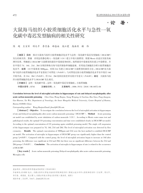
·论　著·大鼠海马组织小胶质细胞活化水平与急性一氧化碳中毒迟发型脑病的相关性研究陈　超　王宝军　项文平　李月春　郝喜娃　庞江霞　高浩然　谢　伟【摘要】　目的　探讨大鼠海马组织小胶质细胞活化水平与急性一氧化碳中毒迟发型脑病（DEACMP）发生的相关性。

方法　采用急性静态吸入一氧化碳（CO）建立中毒大鼠模型，依据Morris水迷宫实验及病理学结果，明确建立DEACMP大鼠模型的最佳中毒浓度和时间；按照最佳中毒浓度再次建立中毒模型，并在中毒后7d、14d、21d、28d分别活体取出海马组织制备单细胞悬液，采用流式细胞仪分析小胶质细胞活化水平。

结果　CO中毒浓度3000ppm、时间21d为建立DEACMP大鼠模型的最佳方法；DEACMP组大鼠海马组织小胶质细胞活化水平显著高于对照组（P<0.05）；与对照组比较小胶质细胞活化水平在中毒后14d开始升高，在21d、28d（P<0.05），但21d、28d组间比较差异无统计学意义（P>0.05）。

结论　大鼠海马组织小胶质细胞活化水平与DEACMP发生相关。

【关键词】　急性一氧化碳中毒；急性一氧化碳中毒迟发型脑病；小胶质细胞中图分类号：R741 文献标识码：A 文章编号：1006-351X（2018）08-0472-04Correlation between the level of microglial activation in hippocampus of rats and delayed encephalopathy afteracute carbon monoxide poisoning Chen Chao, Wang Baojun, Xiang Wenping, Li Yuechun, Hao Xiwa, Pang Jiangxia,Gao Haoran, Xie Wei. Department of Neurology, the Inner Mongolia Medical University, Center Hospital of Baotou,Baotou 014040, ChinaCorresponding author: Wang Baojun:Email: jbwwbj@【Abstract】 Objective To investigate the correlation between the level of microglial activation in hippocampus of rats and delayed encephalopathy after acute carbon monoxide poisoning（DEACMP）. Method Acute poisoning rat model was established by acute inhalation of carbon monoxide（CO）. According to Morris water maze test and pathological results, the optimal CO poisoning concentration and time were established clearly in DEACMP rat model. According to the optimal concentration of CO poisoning again establish poisoning model. The single cell suspension of the hippocampus was prepared in 7d, 14d, 21d and 28d. The level of microglial activation was detected by flow cytometry. Results The optimal concentration of 3000ppm and 21d were the best method to establish DEACMP rat model. The activation of microglia in hippocampus of DEACMP group was significantly higher than the control group （P<0.05） . Compared with the control group, the level of microglial activation began to increase at 14d after poisoning, the difference was significant at 21d and 28d, but there was no significant difference between the 21d and 28d groups （P>0.05）. Conclusion　The activation of microglia in hippocampus of rats is related to the occurrence of DEACMP.【Key words】 Acute carbon monoxide poisoning; Delayed encephalopathy after acute carbon monoxide poisoning; Microglia cells基金项目：国家自然科学基金资助项目（81641040）作者单位：014000 包头，内蒙古医科大学包头临床医学院神经内科（陈超）；包头市中心医院神经内科（王宝军、项文平、李月春、郝喜娃、庞江霞）；内蒙古科技大学包头医学院（高浩然、谢伟）通信作者：王宝军，Email：jbwwbj@一氧化碳（carbon monoxide，CO）中毒可造成以中枢神经系统功能损害为主的多脏器病变［1］，其中急性一氧化碳中毒迟发型脑病（delayed encephalopathy after acute carbon monoxide poisoning，DEACMP）是最常见且严重的并发症［2］，它具有较高的致残率和致死率，严重影响患者生存质量［3］。

季节性模拟条件下中缅树鼩内分泌激素调节作用的研究

季节性模拟条件下中缅树鼩内分泌激素调节作用的研究朱万龙;谢静;蔡金红;王政昆【摘要】In order to investigate the roles of endocrine hormone in the regulation of body mass of Tupaia belangeri,serum leptin lev-els,insulin levels,and the levels of thyroid hormone under simulating winter and summer environments were measured.The results showed that serum leptin levels in T.belangeri in simulating winter environment reduced significantly with the acclamation time;insu-lin levels were significantly correlated to leptin levels,indicating that insulin could positively modulaten and stimulate leptin secretion in T.belangeri;simulating winter environment increased thyroid hormone T 3levels significantly,thereby enhancing the heat production capacity,and simulated summer environment had no obvious influence on the thyroid hormone T3levels,but showed a decreasing trend in a certain extent,weakened the heat production.All of these results suggested that T.belangeri in seasonal change process will be through the adjustment of endocrine hormone levels to regulate the energy metabolism.%为了阐明内分泌激素在中缅树鼩体重调节中的作用,模拟夏季和冬季环境,测定了其血清瘦素含量、胰岛素含量和甲状腺素含量.结果表明:中缅树鼩的血清瘦素水平在模拟冬季环境中显著降低;胰岛素水平与瘦素水平呈显著的正相关,说明中缅树鼩胰岛素能够正向调节和刺激瘦素的分泌;模拟冬季环境显著增加甲状腺素T3含量,从而增强其产热能力,而模拟夏季环境对其影响不大,呈现出降低的趋势,在一定程度上减弱了产热.以上结果说明中缅树鼩在季节性变化过程中会通过调整内分泌激素的含量来调节其能量代谢.【期刊名称】《生物学杂志》【年(卷),期】2017(034)006【总页数】4页(P42-45)【关键词】中缅树鼩;内分泌激素;体重调节【作者】朱万龙;谢静;蔡金红;王政昆【作者单位】云南师范大学生命科学学院云南省高校西南山地生态系统动植物生态适应进化及保护重点实验室,昆明650500;云南师范大学生命科学学院云南省高校西南山地生态系统动植物生态适应进化及保护重点实验室,昆明650500;云南师范大学生命科学学院云南省高校西南山地生态系统动植物生态适应进化及保护重点实验室,昆明650500;云南师范大学生命科学学院云南省高校西南山地生态系统动植物生态适应进化及保护重点实验室,昆明650500【正文语种】中文【中图分类】Q955小型哺乳动物体重的季节性波动主要受到其能量摄入和能量支出的影响[1-2]。

荒漠沙蜥松果体褪黑激素含量的季节性变化

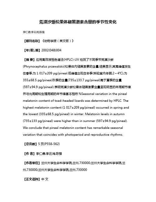
荒漠沙蜥松果体褪黑激素含量的季节性变化李仁德;李云鸿;陈强【期刊名称】《动物学报（英文版）》【年(卷),期】2002(048)004【摘要】应用高效液相色谱法(HPLC)-UV检测了不同季节荒漠沙蜥(Phrynocephalus przewalskii)松果体内褪黑激素的含量.结果显示,其高峰值发生在春季,为1 017±209 pg/pineal.低峰值出现在冬季(实验室内冬眠,2～4℃),为355±68.5 pg/pineal,秋季的含量(735±133.7 pg/pineal)高于夏季的含量(597±94.9 pg/pineal).表明荒漠沙蜥松果体褪黑激素含量呈现明显的年周期节律并与光周期和生殖周期的年节律基本相符.%Seasonal variation in the pineal melatonin content of toad-headed lizards was determined by HPLC. The highest melatonin content (1 017±209 pg/pineal) occurred in spring and the lowest (335±68.5 pg/pineal) in winter. Melatonin levels in autumn (735±133 pg/pineal) were higher than in summer (597±94.9 pg/pineal). We conclude that pineal melatonin content has remarkable seasonal variation that coincides with photoperiod and reproductive rhythms.【总页数】5页(P558-562)【作者】李仁德;李云鸿;陈强【作者单位】兰州大学生命科学学院,兰州,730000;兰州大学生命科学学院,兰州,730000;兰州大学生命科学学院,兰州,730000【正文语种】中文【中图分类】Q95因版权原因，仅展示原文概要，查看原文内容请购买。

北美CHIHUAHUAN荒漠11种啮齿动物种群密度季节性和周期性的比较研究

北美CHIHUAHUAN荒漠11种啮齿动物种群密度季节性和周期性的比较研究曾宗永;杨跃敏【期刊名称】《兽类学报》【年(卷),期】1992(12)3【摘要】本文提出了季节性指标并用时间序列方法分析和比较了北美Chihuahuan荒漠11种啮齿动物种群密度的季节性、趋势和周期性。

结果表明,研究期各年间盘尼西拉特斯颊囊鼠(C.p-enicillatus)有最显著的季节性,鹿鼠属(Peromyscus)的两个物种和伏拉瓦斯囊鼠(Pg.flav-us)的季节性最无规律;11个种群中有7个有趋势,除旗尾更格卢鼠(D.spectabilis)的种群密度呈减少趋势外,其余6个种群的密度呈增加的趋势;种群密度的周期,麦利阿姆更格卢鼠(D.merriami)是4年,曼利卡拉特斯鹿鼠(P.maniculatus)是4.5年,盘尼西拉特斯颊囊鼠(C.penicillatus)等3个种群是1年。

对11个种群的比较说明,这些种群密度的季节性、趋势和周期性呈现出明显的多样化,且与它们的亲缘关系或种系发生历史无显著关系。

11个种群的密度变动的多样化维持了它们在时间方面的共存。

【总页数】10页(P213-222)【作者】曾宗永;杨跃敏【作者单位】不详;不详【正文语种】中文【中图分类】Q959.837【相关文献】1.北美CHIHUAHUAN荒漠啮齿动物群落各物种种群生物量动态的比较研究 [J], 曾宗永;杨跃敏;宋志明2.北美CHIHUAHUAN荒漠啮齿动物群落的能量分配方式 [J], 曾宗永;赵佐成3.北美CHIHUAHUAN荒漠啮齿动物群落动态：Ⅲ.变量的频次分布和预测 [J], 曾宗永;杨跃敏4.北美CHIHUAHUAN荒漠啮齿动物群落动态II.季节性和周期性 [J], 曾宗永;杨跃敏5.北美CHIHUAHUAN荒漠17种啮齿动物的日耗能动态比较 [J], 曾宗永;杨跃敏因版权原因，仅展示原文概要，查看原文内容请购买。

1、下载文档前请自行甄别文档内容的完整性，平台不提供额外的编辑、内容补充、找答案等附加服务。
2、"仅部分预览"的文档,不可在线预览部分如存在完整性等问题,可反馈申请退款(可完整预览的文档不适用该条件!)。
3、如文档侵犯您的权益，请联系客服反馈,我们会尽快为您处理(人工客服工作时间：9:00-18:30)。

图 !" 样点分布图 $%&’ !" 23456738 39 6:; <5-=>78? <76;<"
//：香溪河 /758?@7 A7B;C；01：九冲河 07D4:38? A7B;C；E2：高岚河 E53>58 A7B;C；EF：古夫河 ED9D A7B;C" 下同 G:; <5-; H;>3I"
（ $&$$&!%& ，%&(’!!*’ ）、中国科学院知识 !国家自然科学基金项目创新工程重要方向项目（ Y>J;"7Z47%"’ ）和国家重点基础研究发展规划项目（ "&&"J[%!"$&& ）资助) !!通讯作者) \7P59O：G<C59] 9<T) 5C) C6 "&&+7&*7!( 收稿， "&&*7&!7&. 接受)
!# +" 数据分析方法
%
K:58838VU7;8;C 多样性指数 !" # $ （ ( $ (） [5C?5>;9 # （ >3?* )） A74:8;<< # (
’ & >8’ & " & #(
式中： ( 为分类单元数； ’ & 为第 & 个物种在样本中的相对丰度；) 为样本个数" 本研究中方差分析使用 KZKK ((J ! 软件；典型对应分析（ 11T）使用 158343 +J ! 软件" (" 结果与分析 (# !" 香溪河水系大型底栖动物群落结构
物及其与环境因子间关系的研究相对较少，因此对河流底栖动物开展研究具有重要的生物学和生态学意义) 气候和地理形态特征强烈影响着河流的结构和
’*+
应\ 用\ 生\ 态\ 学\ 报\ \ \ \ \ \ \ \ \ \ \ \ \ \ \ \ \ \ \ *) 卷
［ !］功能 " 气候变化引起整个流域内环境特征包括水
香溪河大型底栖动物群落结构季节动态 !
蒋万祥 # 贾兴焕 # 周淑婵 # 李凤清 # 唐# 涛 # 蔡庆华
!， " !， $ ! ! ! ! !!
（ ! 中国科学院水生生物研究所淡水生态与生物技术国家重点实验室，武汉 %$&&’" ；" 枣庄学院生命科学系，山东枣庄 "’’!(& ；$ 中国林业科学研究院亚热带林业研究所国家林业局杭州湾湿地生态系统定位研究站，浙江富阳 $!!%&& ）
［ (( & (* ］ ,，拥有九冲河、古夫河、高岚河 . 条主要支 *
流" 本研究共设样点 (* 个（图 (） " 于香溪河选取 + 个样点，沿水流方向依次命名为 //*. 、 //*( 、 //($ 和 //(+ ；九冲河选取 ! 个样点，沿水流方向依次命名为 01)’ 、 01)% 、 01)! 、 01). 和 01)* 接影响其他物种的生
［ " , $］存和繁殖，是整个生态系统，特别是水生态系统
物质循环和能量流动的枢纽之一，在一定程度上决定了物质循环和能量流动的方式) 当前我国对底栖
［ %］动物的研究大多集中于湖泊，对于河流中底栖动
) 同时，又
因其取食浮游生物、底栖藻类和有机碎屑等，本身又
摘# 要# 通过大型底栖动物的量化监测，对香溪河水系大型底栖动物季节动态进行研究) 共采集大型底栖动物 !*’ 种，隶属 ( 纲 (+ 科，其中，四节蜉、高翔蜉、短尾石蝇为该水系优势类群，不同季节间大型底栖动物优势类群组成存在较大差异) 大型底栖动物群落结构以冬季最为复杂，春、秋季次之，夏季相对简单) 大型底栖动物功能摄食类群以集食者占优，其次为刮食者、捕食者和滤食者，撕食者丰度最小) 典型对应分析表明，不同季节影响底栖动物群落结构的因子差异较大；夏季和秋季营养盐对底栖动物群落结构影响较大，水深对各季度大型底栖动物群落结构均有影响) 关键词# 香溪河# 大型底栖动物# 季节动态# 功能摄食类群# 典型对应分析文章编号# !&&!,*$$" （ "&&* ） &%,&*"$,&(# 中图分类号# -!’+) .!# 文献标识码# / !"#$%&#’ ()&#*+,$ %- *#,.%/%%0"&12%$ ,%**3&+1) $1.3,13." +& 4+#&56+ 7+8".9 01/23 4567 " $ ! ! ，01/ ;96:7<=56!，，>?@A B<=7C<56! ，D1 EF6:7G96:! ，H/23 H5I! ，J/1 -96:7<=5（ !"#"$ 8956:!， %$& ’#()*#")*& )+ ,*$-./#"$* 01)2)3& #45 67)"$1.4)2)3& ，84-"7"9"$ )+ :&5*)(7)2)3&，;.74$-$ <1#5$= >& )+ !17$41$-， ?9.#4 %$&&’" ， ;.74#； " @$A#*">$4" )+ ’7+$ !17$41$-， B#)C.9#43 D47E$*-7"&， B#)C.9#43 "’’!(& ，!.#45)43，;.74#；$ !"#"$ ,)*$-"*& <5>747-"*#"7)4 ?$"2#45 01)-&-"$> F$-$#*1. !"#"7)4 )+ :#43C.)9 6#&，F$-$#*1. 84-"7"9"$ )+ !9("*)A71#2 ,)*$-"*& ，;.74$-$ <1#5$>& )+ ,)*$-"*& ， ,9&#43 $!!%&& ，B.$G7#43，;.74#） H =;.74H IH <AA2H 01)2) ， "&&* ， :; （%）： *"$,*"+) <0$1.#,1：HI KL=MN L<F KF5KI65O MN65P9CK IQ P5CRISIITF6L<IK CIPP=69LN 96 ;956:89 U9VFR ，L<F 967 M9V9M=5OK IQ P5CRISIITF6L<IK 96 L<F U9VFR WFRF G=56L9L5L9VFON PI69LIRFM) / LIL5O IQ !*’ L585 TFOI6:7 96: LI ( CO5KK 56M (+ Q5P9O9FK WFRF CIOOFCLFM ，5PI6: W<9C<，6#$"7- KXX) ，0A$)*9- KXX) ，56M J$>)9*# KXX) WFRF L<F MIP9656L :RI=XK，56M L<F9R CIPXIK9L9I6K V5R9FM W9L< KF5KI6K) H<F P5CRISI7 ITF6L<IK CIPP=69LN W5K PIKL CIPXO9C5LFM 96 W96LFR ，QIOOIWFM TN 96 KXR96: 56M 5=L=P6 ，56M L<F K9PXOFKL 96 K=PPFR) 35L<FR7CIOOFCLIR W5K L<F P596 CIPXI6F6L IQ Q=6CL9I65O QFFM96: :RI=XK 96 ;9567 :89 U9VFR KNKLFP ，QIOOIWFM TN KCR5XFR，XRFM5LIR，56M Q9OLFR7CIOOFCLIR，W<9OF K<RFMMFR I6ON 5CCI=6LFM QIR 5 KP5OO X5RL) J56I69C5O CIRRFKXI6MF6CF 565ONK9K K<IWFM L<5L L<F Q5CLIRK 5QQFCL96: L<F P5CRISIIT7 F6L<IK CIPP=69LN WFRF M9KK9P9O5R 5PI6: KF5KI6K) 16 K=PPFR 56M 5=L=P6 ，6=LR9F6LK <5M :RF5LFR FQQFCLK；56M 96 5OO KF5KI6K，W5LFR MFXL< <5M MFQ969LF FQQFCLK) =") >%.($：;956:89 U9VFR；P5CRISIITF6L<IK；KF5KI65O MN65P9CK；Q=6CL9I65O QFFM96: :RI=XK；C57 ) 6I69C5O CIRRFKXI6MF6CF 565ONK9K（ JJ/） # # 底栖动物具有相对较长的生命周期、移动能力弱、容易采集、物种易鉴定、具有较高的生物多样性（不同生境中都有分布）和对不同环境有不同敏感度等特点，可作为环境监测的良好指示
［ (! & (# ］学指标均按照国家标准进行测定 "
" 为探索大型底栖动物在河流中的分布规律，