RANDOM SAMPLING - UMBC An Honors University In Maryland随机抽样-马里兰大学在马里兰州的荣誉共57页文档
NLOS identification and mitigation for localization based on UWB experimental data

NLOS Identification and Mitigation for Localization Based on UWB Experimental Data Stefano Maran`o,Student Member,IEEE,Wesley M.Gifford,Student Member,IEEE,Henk Wymeersch,Member,IEEE,Moe Z.Win,Fellow,IEEEAbstract—Sensor networks can benefit greatly from location-awareness,since it allows information gathered by the sensors to be tied to their physical locations.Ultra-wide bandwidth(UWB) transmission is a promising technology for location-aware sensor networks,due to its power efficiency,fine delay resolution,and robust operation in harsh environments.However,the presence of walls and other obstacles presents a significant challenge in terms of localization,as they can result in positively biased distance estimates.We have performed an extensive indoor measurement campaign with FCC-compliant UWB radios to quantify the effect of non-line-of-sight(NLOS)propagation.From these channel pulse responses,we extract features that are representative of the propagation conditions.We then develop classification and regression algorithms based on machine learning techniques, which are capable of:(i)assessing whether a signal was trans-mitted in LOS or NLOS conditions;and(ii)reducing ranging error caused by NLOS conditions.We evaluate the resulting performance through Monte Carlo simulations and compare with existing techniques.In contrast to common probabilistic approaches that require statistical models of the features,the proposed optimization-based approach is more robust against modeling errors.Index Terms—Localization,UWB,NLOS Identification,NLOS Mitigation,Support Vector Machine.I.I NTRODUCTIONL OCATION-AW ARENESS is fast becoming an essential aspect of wireless sensor networks and will enable a myr-iad of applications,in both the commercial and the military sectors[1],[2].Ultra-wide bandwidth(UWB)transmission [3]–[8]provides robust signaling[8],[9],as well as through-wall propagation and high-resolution ranging capabilities[10], [11].Therefore,UWB represents a promising technology for localization applications in harsh environments and accuracy-critical applications[10]–[15].In practical scenarios,however, a number of challenges remain before UWB localization and communication can be deployed.These include signal Manuscript received15May2009;revised15February2010.This research was supported,in part,by the National Science Foundation under grant ECCS-0901034,the Office of Naval Research Presidential Early Career Award for Scientists and Engineers(PECASE)N00014-09-1-0435,the Defense University Research Instrumentation Program under grant N00014-08-1-0826, and the MIT Institute for Soldier Nanotechnologies.S.Maran`o was with Laboratory for Information and Decision Systems (LIDS),Massachusetts Institute of Technology(MIT),and is now with the Swiss Seismological Service,ETH Z¨u rich,Z¨u rich,Switzerland(e-mail: stefano.marano@sed.ethz.ch).H.Wymeersch was with LIDS,MIT,and is now with Chalmers University of Technology,G¨o teborg,Sweden(e-mail:henkw@chalmers.se).Wesley M.Gifford and Moe Z.Win are with LIDS,MIT,Cambridge,MA 02139USA(e-mail:wgifford@,moewin@).Digital Object Identifier10.1109/JSAC.2010.100907.acquisition[16],multi-user interference[17],[18],multipath effects[19],[20],and non-line-of-sight(NLOS)propagation [10],[11].The latter issue is especially critical[10]–[15]for high-resolution localization systems,since NLOS propagation introduces positive biases in distance estimation algorithms, thus seriously affecting the localization performance.Typical harsh environments such as enclosed areas,urban canyons, or under tree canopies inherently have a high occurrence of NLOS situations.It is therefore critical to understand the impact of NLOS conditions on localization systems and to develop techniques that mitigate their effects.There are several ways to deal with ranging bias in NLOS conditions,which we classify as identification and mitigation. NLOS identification attempts to distinguish between LOS and NLOS conditions,and is commonly based on range estimates[21]–[23]or on the channel pulse response(CPR) [24],[25].Recent,detailed overviews of NLOS identification techniques can be found in[22],[26].NLOS mitigation goes beyond identification and attempts to counter the positive bias introduced in NLOS signals.Several techniques[27]–[31]rely on a number of redundant range estimates,both LOS and NLOS,in order to reduce the impact of NLOS range estimates on the estimated agent position.In[32]–[34]the geometry of the environment is explicitly taken into account to cope with NLOS situations.Other approaches,such as[35],attempt to detect the earliest path in the CPR in order to better estimate the TOA in NLOS prehensive overviews of NLOS mitigation techniques can be found in[26],[36]. The main drawbacks of existing NLOS identification and mitigation techniques are:(i)loss of information due to the direct use of ranges instead of the CPRs;(ii)latency incurred during the collection of range estimates to establish a history; and(iii)difficulty in determining the joint probability distribu-tions of the features required by many statistical approaches. In this paper,we consider an optimization-based approach. In particular,we propose the use of non-parametric ma-chine learning techniques to perform NLOS identification and NLOS mitigation.Hence,they do not require a statistical characterization of LOS and NLOS channels,and can perform identification and mitigation under a common framework.The main contributions of this paper are as follows:•characterization of differences in the CPRs under LOS and NLOS conditions based on an extensive indoor mea-surement campaign with FCC-compliant UWB radios;•determination of novel features extracted from the CPR that capture the salient properties in LOS and NLOS conditions;0733-8716/10/$25.00c 2010IEEE•demonstration that a support vector machine (SVM)clas-si fier can be used to distinguish between LOS and NLOS conditions,without the need for statistical modeling of the features under either condition;and•development of SVM regressor-based techniques to mit-igate the ranging bias in NLOS situations,again without the need for statistical modeling of the features under either condition.The remainder of the paper is organized as follows.In Section II,we introduce the system model,problem statement,and describe the effect of NLOS conditions on ranging.In Section III,we describe the equipment and methodologies of the LOS/NLOS measurement campaign and its contribu-tion to this work.The proposed techniques for identi fication and mitigation are described in Section IV,while different strategies for incorporating the proposed techniques within any localization system are discussed in Section V.Numerical performance results are provided in Section VI,and we draw our conclusions in Section VII.II.P ROBLEM S TATEMENT AND S YSTEM M ODEL In this section,we describe the ranging and localization algorithm,and demonstrate the need for NLOS identi fication and mitigation.A.Single-node LocalizationA network consists of two types of nodes:anchors are nodes with known positions,while agents are nodes with unknown positions.For notational convenience,we consider the point of view of a single agent,with unknown position p ,surrounded by N b anchors,with positions,p i ,i =1,...,N b .The distance between the agent and anchor i is d i = p −p i .The agent estimates the distance between itself and the anchors,using a ranging protocol.We denote the estimateddistance between the agent and anchor i by ˆdi ,the ranging error by εi =ˆdi −d i ,the estimate of the ranging error by ˆεi ,the channel condition between the agent and anchor i by λi ∈{LOS ,NLOS },and the estimate of the channelcondition by ˆλi .The mitigated distance estimate of d i is ˆd m i=ˆd i −ˆεi .The residual ranging error after mitigation is de fined as εm i =ˆd m i −d i .Given a set of at least three distance estimates,the agent will then determine its position.While there are numerous positioning algorithms,we focus on the least squares (LS)criterion,due to its simplicity and because it makes no assumptions regarding ranging errors.The agent can infer its position by minimizing the LS cost functionˆp=arg min p(p i ,ˆdi )∈Sˆd i − p −p i 2.(1)Note that we have introduced the concept of the set of useful neighbors S ,consisting of couplesp i ,ˆdi .The optimization problem (1)can be solved numerically using steepest descent.B.Sources of ErrorThe localization algorithm will lead to erroneous results when the ranging errors are large.In practice the estimated distances are not equal to the true distances,because of a number of effects including thermal noise,multipath propa-gation,interference,and ranging algorithm inaccuracies.Ad-ditionally,the direct path between requester and responder may be obstructed,leading to NLOS propagation.In NLOS conditions,the direct path is either attenuated due to through-material propagation,or completely blocked.In the former case,the distance estimates will be positively biased due to the reduced propagation speed (i.e.,less than the expected speed of light,c ).In the latter case the distance estimate is also positively biased,as it corresponds to a re flected path.These bias effects can be accounted for in either the ranging or localization phase.In the remainder of this paper,we focus on techniques that identify and mitigate the effects of NLOS signals during the ranging phase.In NLOS identi fication,the terms in (1)corre-sponding to NLOS distance estimates are omitted.In NLOS mitigation,the distance estimates corresponding to NLOS signals are corrected for improved accuracy.The localization algorithm can then adopt different strategies,depending on the quality and the quantity of available range estimates.III.E XPERIMENTAL A CTIVITIESThis section describes the UWB LOS/NLOS measurement campaign performed at the Massachusetts Institute of Tech-nology by the Wireless Communication and Network Sciences Laboratory during Fall 2007.A.OverviewThe aim of this experimental effort is to build a large database containing a variety of propagation conditions in the indoor of fice environment.The measurements were made using two FCC-compliant UWB radios.These radios repre-sent off-the-shelf transceivers and therefore an appropriate benchmark for developing techniques using currently available technology.The primary focus is to characterize the effects of obstructions.Thus,measurement positions (see Fig.1)were chosen such that half of the collected waveforms were cap-tured in NLOS conditions.The distance between transmitter and receiver varies widely,from roughly 0.6m up to 18m,to capture a variety of operating conditions.Several of fices,hallways,one laboratory,and a large lobby constitute the physical setting of this campaign.While the campaign was conducted in one particular indoor of fice envi-ronment,because of the large number of measurements and the variety of propagation scenarios encountered,we expect that our results are applicable in other of fice environments.The physical arrangement of the campaign is depicted in Fig.1.In each measurement location,the received waveform and the associated range estimate,as well as the actual distance are recorded.The waveforms are then post-processed in order to reduce dependencies on the speci fic algorithm and hardware,e.g.,on the leading edge detection (LED)algorithm embedded in the radios.Fig.1.Measurements were taken in clusters over several different rooms and hallways to capture different propagation conditions.B.Experimental ApparatusThe commercially-available radios used during the data collection process are capable of performing communications and ranging using UWB signals.The radio complies with the emission limit set forth by the FCC[37].Specifically, the10dB bandwidth spans from3.1GHz to6.3GHz.The radio is equipped with a bottom fed planar elliptical antenna. This type of dipole antenna is reported to be well matched and radiation efficient.Most importantly,it is omni-directional and thus suited for ad-hoc networks with arbitrary azimuthal orientation[38].Each radio is mounted on the top of a plastic cart at a height of90cm above the ground.The radios perform a round-trip time-of-arrival(RTOA)ranging protocol1and are capable of capturing waveforms while performing the ranging procedure.Each waveform r(t)captured at the receiving radio is sampled at41.3ps over an observation window of190ns.C.Measurement ArrangementMeasurements were taken at more than one hundred points in the considered area.A map,depicting the topological organization of the clusters within the building,is shown 1RTOA allows ranging between two radios without a common time reference;and thus alleviates the need for networksynchronization.Fig.2.The measurement setup for collecting waveforms between D675CA and H6around the corner of the WCNS Laboratory.in Fig.1,and a typical measurement scenario is shown in Fig.2.Points are placed randomly,but are restricted to areas which are accessible by the carts.The measurement points are grouped into non-overlapping clusters,i.e.,each point only belongs to a single cluster.Typically,a cluster corresponds to a room or a region of a hallway.Within each cluster,measurements between every possible pair of points were captured.When two clusters were within transmission range, every inter-cluster measurement was collected as well.Overall, more than one thousand unique point-to-point measurements were performed.For each pair of points,several received waveforms and distance estimates are recorded,along with the actual distance.During each measurement the radios remain stationary and care is taken to limit movement of other objects in the nearby surroundings.D.DatabaseUsing the measurements collected during the measurement phase,a database was created and used to develop and evaluate the proposed identification and mitigation techniques. It includes1024measurements consisting of512waveforms captured in the LOS condition and512waveforms captured in the NLOS condition.The term LOS is used to denote the existence of a visual path between transmitter and receiver,i.e., a measurement is labeled as LOS when the straight line be-tween the transmitting and receiving antenna is unobstructed. The ranging estimate was obtained by an RTOA algorithm embedded on the radio.The actual position of the radio during each measurement was manually recorded,and the ranging error was calculated with the aid of computer-aided design(CAD)software.The collected waveforms were then processed to align thefirst path in the delay domain using a simple threshold-based method.The alignment process creates a time reference independent of the LED algorithm embedded on the radio.IV.NLOS I DENTIFICATION AND M ITIGATIONThe collected measurement data illustrates that NLOS prop-agation conditions significantly impact ranging performance. For example,Fig.3shows the empirical CDFs of the ranging error over the ensemble of all measurements collected under the two different channel conditions.In LOS conditions a ranging error below one meter occurs in more than95%of the measurements.On the other hand,in NLOS conditions a ranging error below one meter occurs in less than30%of the measurements.Clearly,LOS and NLOS range estimates have very dif-ferent characteristics.In this section,we develop techniques to distinguish between LOS and NLOS situations,and to mitigate the positive biases present in NLOS range estimates. Our techniques are non-parametric,and rely on least-squares support-vector machines(LS-SVM)[39],[40].Wefirst de-scribe the features for distinguishing LOS and NLOS situa-tions,followed by a brief introduction to LS-SVM.We then describe how LS-SVM can be used for NLOS identification and mitigation in localization applications,without needing to determine parametric joint distributions of the features for both the LOS and NLOS conditions.A.Feature Selection for NLOS ClassificationWe have extracted a number of features,which we expect to capture the salient differences between LOS and NLOS signals,from every received waveform r(t).These featuresFig.3.CDF of the ranging error for the LOS and NLOS condition. were selected based on the following observations:(i)in NLOS conditions,signals are considerably more attenuated and have smaller energy and amplitude due to reflections or obstructions;(ii)in LOS conditions,the strongest path of the signal typically corresponds to thefirst path,while in NLOS conditions weak components typically precede the strongest path,resulting in a longer rise time;and(iii)the root-mean-square(RMS)delay spread,which captures the temporal dispersion of the signal’s energy,is larger for NLOS signals. Fig.4depicts two waveforms received in the LOS and NLOS condition supporting our observations.We also include some features that have been presented in the literature.Taking these considerations into account,the features we will consider are as follows:1)Energy of the received signal:E r=+∞−∞|r(t)|2dt(2) 2)Maximum amplitude of the received signal:r max=maxt|r(t)|(3) 3)Rise time:t rise=t H−t L(4) wheret L=min{t:|r(t)|≥ασn}t H=min{t:|r(t)|≥βr max},andσn is the standard deviation of the thermal noise.The values ofα>0and0<β≤1are chosen empirically in order to capture the rise time;in our case, we usedα=6andβ=0.6.4)Mean excess delay:τMED=+∞−∞tψ(t)dt(5) whereψ(t)=|r(t)|2/E r.Fig.4.In some situations there is a clear difference between LOS(upper waveform)and NLOS(lower waveform)signals.5)RMS delay spread:τRMS=+∞−∞(t−τMED)2ψ(t)dt(6)6)Kurtosis:κ=1σ4|r|TT|r(t)|−μ|r|4dt(7)whereμ|r|=1TT|r(t)|dtσ2|r|=1TT|r(t)|−μ|r|2dt.B.Least Squares SVMThe SVM is a supervised learning technique used both for classification and regression problems[41].It represents one of the most widely used classification techniques because of its robustness,its rigorous underpinning,the fact that it requires few user-defined parameters,and its superior performance compared to other techniques such as neural networks.LS-SVM is a low-complexity variation of the standard SVM, which has been applied successfully to classification and regression problems[39],[40].1)Classification:A linear classifier is a function R n→{−1,+1}of the forml(x)=sign[y(x)](8) withy(x)=w Tϕ(x)+b(9) whereϕ(·)is a predetermined function,and w and b are unknown parameters of the classifier.These parameters are de-termined based on the training set{x k,l k}N k=1,where x k∈R n and l k∈{−1,+1}are the inputs and labels,respectively.In the case where the two classes can be separated the SVM determines the separating hyperplane which maximizes the margin between the two classes.2Typically,most practical problems involve classes which are not separable.In this case,the SVM classifier is obtained by solving the following optimization problem:arg minw,b,ξ12w 2+γNk=1ξk(10)s.t.l k y(x k)≥1−ξk,∀k(11)ξk≥0,∀k,(12) where theξk are slack variables that allow the SVM to tolerate misclassifications andγcontrols the trade-off between minimizing training errors and model complexity.It can be shown that the Lagrangian dual is a quadratic program(QP) [40,eqn.2.26].To further simplify the problem,the LS-SVM replaces the inequality(11)by an equality:arg minw,b,e12w 2+γ12Nk=1e2k(13)s.t.l k y(x k)=1−e k,∀k.(14) Now,the Lagrangian dual is a linear program(LP)[40,eqn.3.5],which can be solved efficiently by standard optimization toolboxes.The resulting classifier can be written asl(x)=signNk=1αk l k K(x,x k)+b,(15)whereαk,the Lagrange multipliers,and b are found from the solution of the Lagrangian dual.The function K(x k,x l)=ϕ(x k)Tϕ(x l)is known as the kernel which enables the SVM to perform nonlinear classification.2)Regression:A linear regressor is a function R n→R of the formy(x)=w Tϕ(x)+b(16) whereϕ(·)is a predetermined function,and w and b are unknown parameters of the regressor.These parameters are determined based on the training set{x k,y k}N k=1,where x k∈R n and y k∈R are the inputs and outputs,respectively. The LS-SVM regressor is obtained by solving the following optimization problem:arg minw,b,e12w 2+γ12e 2(17)s.t.y k=y(x k)+e k,∀k,(18) whereγcontrols the trade-off between minimizing training errors and model complexity.Again,the Lagrangian dual is an LP[40,eqn.3.32],whose solution results in the following LS-SVM regressory(x)=Nk=1αk K(x,x k)+b.(19)2The margin is given by1/ w ,and is defined as the smallest distance between the decision boundary w Tϕ(x)+b=0and any of the training examplesϕ(x k).C.LS-SVM for NLOS Identi fication and MitigationWe now apply the non-parametric LS-SVM classi fier to NLOS identi fication,and the LS-SVM regressor to NLOS mitigation.We use 10-fold cross-validation 3to assess the performance of our features and the SVM.Not only are we interested in the performance of LS-SVM for certain features,but we are also interested in which subsets of the available features give the best performance.1)Classi fication:To distinguish between LOS and NLOS signals,we train an LS-SVM classi fier with inputs x k and corresponding labels l k =+1when λk =LOS and l k =−1when λk =NLOS .The input x k is composed of a subset of the features given in Section IV-A.A trade-off between classi fier complexity and performance can be made by using a different size feature subset.2)Regression:To mitigate the effect of NLOS propagation,we train an LS-SVM regressor with inputs x k and corre-sponding outputs y k =εk associated with the NLOS signals.Similar to the classi fication case,x k is composed of a subset of features,selected from those given in Section IV-A and therange estimate ˆdk .Again,the performance achieved by the regressor will depend on the size of the feature subset and the combination of features used.V.L OCALIZATION S TRATEGIESBased on the LS-SVM classi fier and regressor,we can develop the following localization strategies:(i)localization via identi fication ,where only classi fication is employed;(ii)localization via identi fication and mitigation ,where the re-ceived waveform is first classi fied and error mitigation is performed only on the range estimates from those signals identi fied as NLOS;and (iii)a hybrid approach which discards mitigated NLOS range estimates when a suf ficient number of LOS range estimates are present.A.Strategy 1:StandardIn the standard strategy,all the range estimates ˆdi from neighboring anchor nodes are used by the LS algorithm (1)for localization.In other words,S S =p i ,ˆd i :1≤i ≤N b .(20)B.Strategy 2:Identi ficationIn the second strategy,waveforms are classi fied as LOS or NLOS using the LS-SVM classi fier.Range estimates are used by the localization algorithm only if the associated waveform was classi fied as LOS,while range estimates from waveforms classi fied as NLOS are discarded:S I = p i ,ˆd i:1≤i ≤N b ,ˆλi =LOS .(21)Whenever the cardinality of S I is less than three,the agent isunable to localize.4In this case,we set the localization error to +∞.3InK -fold cross-validation,the dataset is randomly partitioned into K parts of approximately equal size,each containing 50%LOS and 50%NLOS waveforms.The SVM is trained on K −1parts and the performance is evaluated on the remaining part.This is done a total of K times,using each of the K parts exactly once for evaluation and K −1times for training.4Note that three is the minimum number of anchor nodes needed to localize in two-dimensions.TABLE IF ALSE ALARM PROBABILITY (P F ),MISSED DETECTION PROBABILITY (P M ),AND OVERALL ERROR PROBABILITY (P E )FOR DIFFERENT NLOSIDENTIFICATION TECHNIQUES .T HE SET F i IDENOTES THE SET OF i FEATURES WITH THE SMALLEST P E USING THE LS-SVM TECHNIQUE .Identi fication Technique P F P M P E Parametric technique given in [42]0.1840.1430.164LS-SVM using features from [42]0.1290.1520.141F 1I ={r max }0.1370.1230.130F 2I ={r max ,t rise }0.0920.1090.100F 3I ={E r ,t rise ,κ}0.0820.0900.086F 4I={E r ,r max ,t rise ,κ}0.0820.0900.086F 5I ={E r ,r max ,t rise ,τMED ,κ}0.0860.0900.088F 6I={E r ,r max ,t rise ,τMED ,τRMS ,κ}0.0920.0900.091C.Strategy 3:Identi fication and MitigationThis strategy is an extension to the previous strategy,wherethe received waveform is first classi fied as LOS or NLOS,and then the mitigation algorithm is applied to those signals with ˆλi =NLOS .For this case S IM =S I ∪S M ,where S M = p i ,ˆd m i :1≤i ≤N b ,ˆλi =NLOS ,(22)and the mitigated range estimate ˆd m iis described in Sec.II.This approach is motivated by the observation that mitigation is not necessary for range estimates associated with LOS waveforms,since their accuracy is suf ficiently high.D.Strategy 4:Hybrid Identi fication and Mitigation In the hybrid approach,range estimates are mitigated as in the previous strategy.However,mitigated range estimates are only used when less than three LOS anchors are available:5S H =S I if |S I |≥3S IMotherwise(23)This approach is motivated by the fact that mitigated range es-timates are often still less accurate than LOS range estimates.Hence,only LOS range estimates should be used,unless there is an insuf ficient number of them to make an unambiguous location estimate.VI.P ERFORMANCE E VALUATION AND D ISCUSSION In this section,we quantify the performance of the LS-SVM classi fier and regressor from Section IV,as well as the four localization strategies from Section V.We will first consider identi fication,then mitigation,and finally localization.For every technique,we will provide the relevant performance measures as well as the quantitative details of how the results were obtained.5Inpractice the angular separation of the anchors should be suf ficiently large to obtain an accurate estimate.If this is not the case,more than three anchors may be needed.TABLE IIM EAN AND RMS VALUES OF RRE FOR LS-SVM REGRESSION -BASEDMITIGATION .T HE SET F i MDENOTES THE SET OF i FEATURES WHICH ACHIEVES THE MINIMUM RMS RRE.Mitigation Technique with LS-SVM RegressionMean [m]RMS [m ]No Mitigation2.63223.589F 1M={ˆd}-0.0004 1.718F 2M ={κ,ˆd }-0.0042 1.572F 3M ={t rise ,κ,ˆd }0.0005 1.457F 4M ={t rise ,τMED ,κ,ˆd }0.0029 1.433F 5M={E r ,t rise ,τMED ,κ,ˆd }0.0131 1.425F 6M ={E r ,t rise ,τMED ,τRMS ,κ,ˆd }0.0181 1.419F 7M={E r ,r max ,t rise ,τMED ,τRMS ,κ,ˆd}0.01801.425A.LOS/NLOS Identi ficationIdenti fication results,showing the performance 6for eachfeature set size,are given in Table I.For the sake of compari-son,we also evaluate the performance of the parametric identi-fication technique from [42],which relies on three features:the mean excess delay,the RMS delay spread,and the kurtosis of the waveform.For fair comparison,these features are extracted from our database.The performance is measured in terms of the misclassi fication rate:P E =(P F +P M )/2,where P F is the false alarm probability (i.e.,deciding NLOS when the signal was LOS),and P M is the missed detection probability (i.e.,deciding LOS when the signal was NLOS).The table only lists the feature sets which achieved the minimum misclassi fication rate for each feature set size.We observe that the LS-SVM,using the three features from [42],reduces the false alarm probability compared to the parametric technique.It was shown in [43]that the features from [42],in fact,give rise to the worst performance among all possible sets of size three considered ing the features from Section IV-A and considering all feature set sizes,our results indicate that the feature set of size three,F 3I ={E r ,t rise ,κ},provides the best pared to the parametric technique,this set reduces both the false alarm and missed detection probabilities and achieves a correct classi fication rate of above 91%.In particular,among all feature sets of size three (results not shown,see [43]),there are seven sets that yield a P E of roughly 10%.All seven of these sets have t rise in common,while four have r max in common,indicating that these two features play an important role.Their importance is also corroborated by the presence of r max and t rise in the selected sets listed in Table I.For the remainder of this paper we will use the feature set F 3I for identi fication.B.NLOS MitigationMitigation results,showing the performance 7for different feature set sizes are given in Table II.The performance is measured in terms of the root mean square residual ranging6Wehave used an RBF kernel of the form K (x ,x k )=exp “− x −x k 2”and set γ=0.1.Features are first converted to the log domain in order to reduce the dynamic range.7Here we used a kernel given by K (x ,x k )=exp “− x −x k2/162”and set γ=10.Again,features are first converted to the log domain.Fig.5.CDF of the ranging error for the NLOS case,before and after mitigation.error (RMS RRE): 1/N N i =1(εm i )2.A detailed analysis ofthe experimental data indicates that large range estimates are likely to exhibit large positive ranging errors.This means that ˆditself is a useful feature,as con firmed by the presence of ˆdin all of the best feature sets listed in the table.Increasing the feature set size can further improve the RMS RRE.Thefeature set of size six,F 6M={E r ,t rise ,τMED ,τRMS ,κ,ˆd },offers the best performance.For the remainder of this paper,we will use this feature set for NLOS mitigation.Fig.5shows the CDF of the ranging error before and after mitigation using this feature set.We observe that without mitigation around 30%of the NLOS waveforms achieved an accuracy of less than one meter (|ε|<1).Whereas,after the mitigation process,60%of the cases have an accuracy less than 1m.C.Localization Performance1)Simulation Setup:We evaluate the localization perfor-mance for fixed number of anchors (N b )and a varying prob-ability of NLOS condition 0≤P NLOS ≤1.We place an agent at a position p =(0,0).For every anchor i (1≤i ≤N b ),we draw a waveform from the database:with probability P NLOS we draw from the NLOS database and with probability 1−P NLOS from the LOS database.The true distance d i corre-sponding to that waveform is then used to place the i th anchor at position p i =(d i sin(2π(i −1)/N b ),d i cos(2π(i −1)/N b )),while the estimated distance ˆdi is provided to the agent.This creates a scenario where the anchors are located at different distances from the agent with equal angular spacing.The agent estimates its position,based on a set of useful neighbors S ,using the LS algorithm from Section II.The arithmetic mean 8of the anchor positions is used as the initial estimate of the agent’s position.2)Performance Measure:To capture the accuracy and availability of localization,we introduce the notion of outage probability .For a certain scenario (N b and P NLOS )and a8Thisis a fair setting for the simulation,as all the strategies are initialized inthe same way.Indeed,despite the identical initialization,strategies converge to signi ficantly different final position estimates.In addition,we note that such an initial position estimate is always available to the agent.。
!How Far are We from Solving Pedestrian Detection
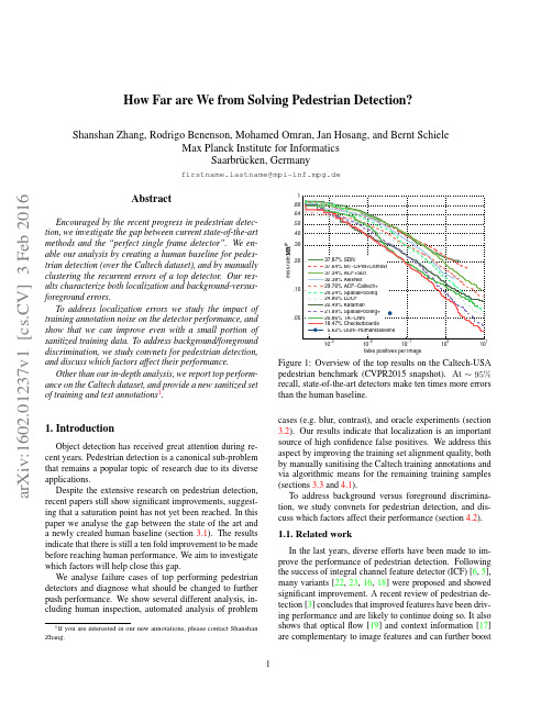
from Solving Pedestrian Detection?Mohamed Omran,Jan Hosang,and Bernt SchielePlanck Institute for Informatics Saarbrücken,Germanystname@mpi-inf.mpg.deAbstractEncouraged by the recent progress in pedestrian detec-tion,we investigate the gap between current state-of-the-art methods and the “perfect single frame detector”.We en-able our analysis by creating a human baseline for pedes-trian detection (over the Caltech dataset),and by manually clustering the recurrent errors of a top detector.Our res-ults characterize both localization and background-versus-foreground errors.To address localization errors we study the impact of training annotation noise on the detector performance,and show that we can improve even with a small portion of sanitized training data.To address background/foreground discrimination,we study convnets for pedestrian detection,and discuss which factors affect their performance.Other than our in-depth analysis,we report top perform-ance on the Caltech dataset,and provide a new sanitized set of training and test annotations 1.1.IntroductionObject detection has received great attention during re-cent years.Pedestrian detection is a canonical sub-problem that remains a popular topic of research due to its diverse applications.Despite the extensive research on pedestrian detection,recent papers still show significant improvements,suggest-ing that a saturation point has not yet been reached.In this paper we analyse the gap between the state of the art and a newly created human baseline (section 3.1).The results indicate that there is still a ten fold improvement to be made before reaching human performance.We aim to investigate which factors will help close this gap.We analyse failure cases of top performing pedestrian detectors and diagnose what should be changed to further push performance.We show several different analysis,in-cluding human inspection,automated analysis of problem1Ifyou are interested in our new annotations,please contact Shanshan Zhang.1010101010Figure 1:Overview of the top results on the Caltech-USA pedestrian benchmark (CVPR2015snapshot).At ∼95%recall,state-of-the-art detectors make ten times more errors than the human baseline.cases (e.g.blur,contrast),and oracle experiments (section 3.2).Our results indicate that localization is an important source of high confidence false positives.We address this aspect by improving the training set alignment quality,both by manually sanitising the Caltech training annotations and via algorithmic means for the remaining training samples (sections 3.3and 4.1).To address background versus foreground discrimina-tion,we study convnets for pedestrian detection,and dis-cuss which factors affect their performance (section 4.2).1.1.Related workIn the last years,diverse efforts have been made to im-prove the performance of pedestrian detection.Following the success of integral channel feature detector (ICF)[6,5],many variants [22,23,16,18]were proposed and showed significant improvement.A recent review of pedestrian de-tection [3]concludes that improved features have been driv-ing performance and are likely to continue doing so.It also shows that optical flow [19]and context information [17]are complementary to image features and can further boost 1a r X i v :1602.01237v 1 [c s .C V ] 3 F eb 2016detection accuracy.Byfine-tuning a model pre-trained on external data convolution neural networks(convnets)have also reached state-of-the-art performance[15,20].Most of the recent papers focus on introducing novelty and better results,but neglect the analysis of the resulting system.Some analysis work can be found for general ob-ject detection[1,14];in contrast,in thefield of pedestrian detection,this kind of analysis is rarely done.In2008,[21] provided a failure analysis on the INRIA dataset,which is relatively small.The best method considered in the2012 Caltech dataset survey[7]had10×more false positives at20%recall than the methods considered here,and no method had reached the95%mark.Since pedestrian detection has improved significantly in recent years,a deeper and more comprehensive analysis based on state-of-the-art detectors is valuable to provide better understanding as to where future efforts would best be invested.1.2.ContributionsOur key contributions are as follows:(a)We provide a detailed analysis of a state-of-the-art ped-estrian detection system,providing insights into failure cases.(b)We provide a human baseline for the Caltech Pedestrian Benchmark;as well as a sanitised version of the annotations to serve as new,high quality ground truth for the training and test sets of the benchmark.The data will be public. (c)We analyse how much the quality of training data affects the detector.More specifically we quantify how much bet-ter alignment and fewer annotation mistakes can improve performance.(d)Using the insights of the analysis,we explore variants of top performing methods:filtered channel feature detector [23]and R-CNN detector[13,15],and show improvements over the baselines.2.PreliminariesBefore delving into our analysis,let us describe the data-sets in use,their metrics,and our baseline detector.2.1.Caltech-USA pedestrian detection benchmarkAmongst existing pedestrian datasets[4,9,8],KITTI [11]and Caltech-USA are currently the most popular ones. In this work we focus on the Caltech-USA benchmark[7] which consists of2.5hours of30Hz video recorded from a vehicle traversing the streets of Los Angeles,USA.The video annotations amount to a total of350000bound-ing boxes covering∼2300unique pedestrians.Detec-tion methods are evaluated on a test set consisting of4024 frames.The provided evaluation toolbox generates plotsFilter type MR O−2ACF[5]44.2SCF[3]34.8LDCF[16]24.8RotatedFilters19.2Checkerboards18.5Table1:Thefiltertype determines theICF methods quality.Base detector MR O−2+Context+FlowOrig.2Ped[17]48~5pp/Orig.SDt[19]45/8ppSCF[3]355pp4ppCheckerboards19~01ppTable2:Detection quality gain ofadding context[17]and opticalflow[19],as function of the base detector.for different subsets of the test set based on annotation size, occlusion level and aspect ratio.The established proced-ure for training is to use every30th video frame which res-ults in a total of4250frames with∼1600pedestrian cut-outs.More recently,methods which can leverage more data for training have resorted to afiner sampling of the videos [16,23],yielding up to10×as much data for training than the standard“1×”setting.MR O,MR N In the standard Caltech evaluation[7]the miss rate(MR)is averaged over the low precision range of [10−2,100]FPPI.This metric does not reflect well improve-ments in localization errors(lowest FPPI range).Aiming for a more complete evaluation,we extend the evaluation FPPI range from traditional[10−2,100]to[10−4,100],we denote these MR O−2and MR O−4.O stands for“original an-notations”.In section3.3we introduce new annotations, and mark evaluations done there as MR N−2and MR N−4.We expect the MR−4metric to become more important as de-tectors get stronger.2.2.Filtered channel features detectorFor the analysis in this paper we consider all methods published on the Caltech Pedestrian benchmark,up to the last major conference(CVPR2015).As shown infigure1, the best method at the time is Checkerboards,and most of the top performing methods are of its same family.The Checkerboards detector[23]is a generalization of the Integral Channels Feature detector(ICF)[6],which filters the HOG+LUV feature channels before feeding them into a boosted decision forest.We compare the performance of several detectors from the ICF family in table1,where we can see a big improve-ment from44.2%to18.5%MR O−2by introducingfilters over the feature channels and optimizing thefilter bank.Current top performing convnets methods[15,20]are sensitive to the underlying detection proposals,thus wefirst focus on the proposals by optimizing thefiltered channel feature detectors(more on convnets in section4.2). Rotatedfilters For the experiments involving train-ing new models(in section 4.1)we use our own re-implementation of Checkerboards[23],based on the LDCF[16]codebase.To improve the training time we decrease the number offilters from61in the originalCheckerboards down to9filters.Our so-called Rota-tedFilters are a simplified version of LDCF,applied at three different scales(in the same spirit as Squares-ChnFtrs(SCF)[3]).More details on thefilters are given in the supplementary material.As shown in table1,Ro-tatedFilters are significantly better than the original LDCF,and only1pp(percent point)worse than Checker-boards,yet run6×faster at train and test time. Additional cues The review[3]showed that context and opticalflow information can help improve detections. However,as the detector quality improves(table1)the re-turns obtained from these additional cues erodes(table2). Without re-engineering such cues,gains in detection must come from the core detector.3.Analysing the state of the artIn this section we estimate a lower bound on the re-maining progress available,analyse the mistakes of current pedestrian detectors,and propose new annotations to better measure future progress.3.1.Are we reaching saturation?Progress on pedestrian detection has been showing no sign of slowing in recent years[23,20,3],despite recent im-pressive gains in performance.How much progress can still be expected on current benchmarks?To answer this ques-tion,we propose to use a human baseline as lower bound. We asked domain experts to manually“detect”pedestrians in the Caltech-USA test set;machine detection algorithms should be able to at least reach human performance and, eventually,superhuman performance.Human baseline protocol To ensure a fair comparison with existing detectors,we focus on the single frame mon-ocular detection setting.Frames are presented to annotators in random order,and without access to surrounding frames from the source videos.Annotators have to rely on pedes-trian appearance and single-frame context rather than(long-term)motion cues.The Caltech benchmark normalizes the aspect ratio of all detection boxes[7].Thus our human annotations are done by drawing a line from the top of the head to the point between both feet.A bounding box is then automatically generated such that its centre coincides with the centre point of the manually-drawn axis,see illustration infigure2.This procedure ensures the box is well centred on the subject (which is hard to achieve when marking a bounding box).To check for consistency among the two annotators,we produced duplicate annotations for a subset of the test im-ages(∼10%),and evaluated these separately.With a Intersection over Union(IoU)≥0.5matching criterion, the results were identical up to a single boundingbox.Figure2:Illustration of bounding box generation for human baseline.The annotator only needs to draw a line from the top of the head to the central point between both feet,a tight bounding box is then automatically generated. Conclusion Infigure3,we compare our human baseline with other top performing methods on different subsets of the test data(varying height ranges and occlu-sion levels).Wefind that the human baseline widely out-performs state-of-the-art detectors in all settings2,indicat-ing that there is still room for improvement for automatic methods.3.2.Failure analysisSince there is room to grow for existing detectors,one might want to know:when do they fail?In this section we analyse detection mistakes of Checkerboards,which obtains top performance on most subsets of the test set(see figure3).Since most top methods offigure1are of the ICF family,we expect a similar behaviour for them too.Meth-ods using convnets with proposals based on ICF detectors will also be affected.3.2.1Error sourcesThere are two types of errors a detector can do:false pos-itives(detections on background or poorly localized detec-tions)and false negatives(low-scoring or missing pedes-trian detections).In this analysis,we look into false positive and false negative detections at0.1false positives per im-age(FPPI,1false positive every10images),and manually cluster them(one to one mapping)into visually distinctive groups.A total of402false positive and148false negative detections(missing recall)are categorized by error type. False positives After inspection,we end up having all false positives clustered in eleven categories,shown infig-ure4a.These categories fall into three groups:localization, background,and annotation errors.Background errors are the most common ones,mainly ver-tical structures(e.g.figure5b),tree leaves,and traffic lights. This indicates that the detectors need to be extended with a better vertical context,providing visibility over larger struc-tures and a rough height estimate.Localization errors are dominated by double detections2Except for IoU≥0.8.This is due to issues with the ground truth, discussed in section3.3.Reasonable (IoU >= 0.5)Height > 80Height in [50,80]Height in [30,50]020406080100HumanBaselineCheckerboards RotatedFiltersm i s s r a t eFigure 3:Detection quality (log-average miss rate)for different test set subsets.Each group shows the human baseline,the Checkerboards [23]and RotatedFilters detectors,as well as the next top three (unspecified)methods (different for each setting).The corresponding curves are provided in the supplementary material.(high scoring detections covering the same pedestrian,e.g.figure 5a ).This indicates that improved detectors need to have more localized responses (peakier score maps)and/or a different non-maxima suppression strategy.In sections 3.3and 4.1we explore how to improve the detector localiz-ation.The annotation errors are mainly missing ignore regions,and a few missing person annotations.In section 3.3we revisit the Caltech annotations.False negatives Our clustering results in figure 4b show the well known difficulty of detecting small and oc-cluded objects.We hypothesise that low scoring side-view persons and cyclists may be due to a dataset bias,i.e.these cases are under-represented in the training set (most per-sons are non-cyclist walking on the side-walk,parallel to the car).Augmenting the training set with external images for these cases might be an effective strategy.To understand better the issue with small pedestrians,we measure size,blur,and contrast for each (true or false)de-tection.We observed that small persons are commonly sat-urated (over or under exposed)and blurry,and thus hypo-thesised that this might be an underlying factor for weak detection (other than simply having fewer pixels to make the decision).Our results indicate however that this is not the case.As figure 4c illustrates,there seems to be no cor-relation between low detection score and low contrast.This also holds for the blur case,detailed plots are in the sup-plementary material.We conclude that the small number of pixels is the true source of difficulty.Improving small objects detection thus need to rely on making proper use of all pixels available,both inside the window and in the surrounding context,as well as across time.Conclusion Our analysis shows that false positive er-rors have well defined sources that can be specifically tar-geted with the strategies suggested above.A fraction of the false negatives are also addressable,albeit the small and oc-cluded pedestrians remain a (hard and)significant problem.20406080100120# e r r o r s 0100200300loc a liz a tion ba c k g round a nnota e rrors#e r r o r s (a)False positive sources15304560# e r r o r s (b)False negative sources(c)Contrast versus detection scoreFigure 4:Errors analysis of Checkerboards [23]on the test set.(a)double detectionFigure 5:Example of analysed false positive cases (red box).Additional ones in supplementary material.3.2.2Oracle test casesThe analysis of section 3.2.1focused on errors counts.For area-under-the-curve metrics,such astheones used in Caltech,high-scoring errors matter more than low-scoring ones.In this section we directly measure the impact of loc-alization and background-vs-foreground errors on the de-tection quality metric (log-average miss-rate)by using or-acle test cases.In the oracle case for localization,all false positives that overlap with ground truth are ignored for evaluation.In the oracle tests for background-vs-foreground,all false posit-ives that do not overlap with ground truth are ignored.Figure 6a shows that fixing localization mistakes im-proves performance in the low FPPI region;while fixing background mistakes improves results in the high FPPI re-gion.Fixing both types of mistakes results zero errors,even though this is not immediately visible due to the double log plot.In figure 6b we show the gains to be obtained in MR O −4terms by fixing localization or background issues.When comparing the eight top performing methods we find that most methods would boost performance significantly by fix-ing either problem.Note that due to the log-log nature of the numbers,the sum of localization and background deltas do not add up to the total miss-rate.Conclusion For most top performing methods localiz-ation and background-vs-foreground errors have equal im-pact on the detection quality.They are equally important.3.3.Improved Caltech-USA annotationsWhen evaluating our human baseline (and other meth-ods)with a strict IoU ≥0.8we notice in figure 3that the performance drops.The original annotation protocol is based on interpolating sparse annotations across multiple frames [7],and these sparse annotations are not necessar-ily located on the evaluated frames.After close inspection we notice that this interpolation generates a systematic off-set in the annotations.Humans walk with a natural up and down oscillation that is not modelled by the linear interpol-ation used,thus in most frames have shifted bounding box annotations.This effect is not noticeable when using the forgiving IoU ≥0.5,however such noise in the annotations is a hurdle when aiming to improve object localization.1010−210−110010false positives per image18.47(33.20)% Checkerboards15.94(25.49)% Checkerboards (localization oracle)11.92(26.17)% Checkerboards (background oracle)(a)Original and two oracle curves for Checkerboards de-tector.Legend indicates MR O −2 MR O −4 .(b)Comparison of miss-rate gain (∆MR O −4)for top performing methods.Figure 6:Oracle cases evaluation over Caltech test set.Both localization and background-versus-foreground show important room for improvement.(a)False annotations (b)Poor alignmentFigure 7:Examples of errors in original annotations.New annotations in green,original ones in red.This localization issues together with the annotation er-rors detected in section 3.2.1motivated us to create a new set of improved annotations for the Caltech pedestrians dataset.Our aim is two fold;on one side we want to provide a more accurate evaluation of the state of the art,in particu-lar an evaluation suitable to close the “last 20%”of the prob-lem.On the other side,we want to have training annotations and evaluate how much improved annotations lead to better detections.We evaluate this second aspect in section 4.1.New annotation protocol Our human baseline focused on a fair comparison with single frame methods.Our new annotations are done both on the test and training 1×set,and focus on high quality.The annotators are allowed to look at the full video to decide if a person is present or not,they are request to mark ignore regions in areas cov-ering crowds,human shapes that are not persons (posters,statues,etc.),and in areas that could not be decided as cer-tainly not containing a person.Each person annotation is done by drawing a line from the top of the head to the point between both feet,the same as human baseline.The annot-ators must hallucinate head and feet if these are not visible. When the person is not fully visible,they must also annotate a rectangle around the largest visible region.This allows to estimate the occlusion level in a similar fashion as the ori-ginal Caltech annotations.The new annotations do share some bounding boxes with the human baseline(when no correction was needed),thus the human baseline cannot be used to do analysis across different IoU thresholds over the new test set.In summary,our new annotations differ from the human baseline in the following aspects:both training and test sets are annotated,ignore regions and occlusions are also an-notated,full video data is used for decision,and multiple revisions of the same image are allowed.After creating a full independent set of annotations,we con-solidated the new annotations by cross-validating with the old annotations.Any correct old annotation not accounted for in the new set,was added too.Our new annotations correct several types of errors in the existing annotations,such as misalignments(figure 7b),missing annotations(false negatives),false annotations (false positives,figure7a),and the inconsistent use of“ig-nore”regions.Our new annotations will be publicly avail-able.Additional examples of“original versus new annota-tions”provided in the supplementary material,as well as visualization software to inspect them frame by frame. Better alignment In table3we show quantitative evid-ence that our new annotations are at least more precisely localized than the original ones.We summarize the align-ment quality of a detector via the median IoU between true positive detections and a give set of annotations.When evaluating with the original annotations(“median IoU O”column in table3),only the model trained with original annotations has good localization.However,when evalu-ating with the new annotations(“median IoU N”column) both the model trained on INRIA data,and on the new an-notations reach high localization accuracy.This indicates that our new annotations are indeed better aligned,just as INRIA annotations are better aligned than Caltech.Detailed IoU curves for multiple detectors are provided in the supplementary material.Section4.1describes the RotatedFilters-New10×entry.4.Improving the state of the artIn this section we leverage the insights of the analysis, to improve localization and background-versus-foreground discrimination of our baseline detector.DetectorTrainingdataMedianIoU OMedianIoU N Roerei[2]INRIA0.760.84RotatedFilters Orig.10×0.800.77RotatedFilters New10×0.760.85 Table3:Median IoU of true positives for detectors trained on different data,evaluated on original and new Caltech test.Models trained on INRIA align well with our new an-notations,confirming that they are more precise than previ-ous ones.Curves for other detectors in the supplement.Detector Anno.variant MR O−2MR N−2ACFOriginal36.9040.97Pruned36.4135.62New41.2934.33 RotatedFiltersOriginal28.6333.03Pruned23.8725.91New31.6525.74 Table4:Effects of different training annotations on detec-tion quality on validation set(1×training set).Italic num-bers have matching training and test sets.Both detectors im-prove on the original annotations,when using the“pruned”variant(see§4.1).4.1.Impact of training annotationsWith new annotations at hand we want to understand what is the impact of annotation quality on detection qual-ity.We will train ACF[5]and RotatedFilters mod-els(introduced in section2.2)using different training sets and evaluate on both original and new annotations(i.e. MR O−2,MR O−4and MR N−2,MR N−4).Note that both detect-ors are trained via boosting and thus inherently sensitive to annotation noise.Pruning benefits Table4shows results when training with original,new and pruned annotations(using a5/6+1/6 training and validation split of the full training set).As ex-pected,models trained on original/new and tested on ori-ginal/new perform better than training and testing on differ-ent annotations.To understand better what the new annota-tions bring to the table,we build a hybrid set of annotations. Pruned annotations is a mid-point that allows to decouple the effects of removing errors and improving alignment. Pruned annotations are generated by matching new and ori-ginal annotations(IoU≥0.5),marking as ignore region any original annotation absent in the new ones,and adding any new annotation absent in the original ones.From original to pruned annotations the main change is re-moving annotation errors,from pruned to new,the main change is better alignment.From table4both ACF and RotatedFilters benefit from removing annotation er-rors,even in MR O−2.This indicates that our new training setFigure 8:Examples of automatically aligned ground truth annotations.Left/right →before/after alignment.1×data 10×data aligned withMR O −2(MR O −4)MR N −2(MR N−4)Orig.Ø19.20(34.28)17.22(31.65)Orig.Orig.10×19.16(32.28)15.94(29.33)Orig.New 1/2×16.97(28.01)14.54(25.06)NewNew 1×16.77(29.76)12.96(22.20)Table 5:Detection quality of RotatedFilters on test set when using different aligned training sets.All mod-els trained with Caltech 10×,composed with different 1×+9×combinations.is better sanitized than the original one.We see in MR N −2that the stronger detector benefits more from better data,and that the largest gain in detection qual-ity comes from removing annotation errors.Alignment benefits The detectors from the ICF family benefit from training with increased training data [16,23],using 10×data is better than 1×(see section 2.1).To lever-age the 9×remaining data using the new 1×annotations we train a model over the new annotations and use this model to re-align the original annotations over the 9×portion.Be-cause the new annotations are better aligned,we expect this model to be able to recover slight position and scale errors in the original annotations.Figure 8shows example results of this process.See supplementary material for details.Table 5reports results using the automatic alignment pro-cess,and a few degraded cases:using the original 10×,self-aligning the original 10×using a model trained over original 10×,and aligning the original 10×using only a fraction of the new annotations (without replacing the 1×portion).The results indicate that using a detector model to improve overall data alignment is indeed effective,and that better aligned training data leads to better detection quality (both in MR O and MR N ).This is in line with the analysis of section 3.2.Already using a model trained on 1/2of the new annotations for alignment,leads to a stronger model than obtained when using original annotations.We name the RotatedFilters model trained using the new annotations and the aligned 9×data,Rotated-Filters-New10×.This model also reaches high me-dian true positives IoU in table 3,indicating that indeed it obtains more precise detections at test time.Conclusion Using high quality annotations for training improves the overall detection quality,thanks both to im-proved alignment and to reduced annotation errors.4.2.Convnets for pedestrian detectionThe results of section 3.2indicate that there is room for improvement by focusing on the core background versus foreground discrimination task (the “classification part of object detection”).Recent work [15,20]showed compet-itive performance with convolutional neural networks (con-vnets)for pedestrian detection.We include convnets into our analysis,and explore to what extent performance is driven by the quality of the detection proposals.AlexNet and VGG We consider two convnets.1)The AlexNet from [15],and 2)The VGG16model from [12].Both are pre-trained on ImageNet and fine-tuned over Cal-tech 10×(original annotations)using SquaresChnFtrs proposals.Both networks are based on open source,and both are instances of the R-CNN framework [13].Albeit their training/test time architectures are slightly different (R-CNN versus Fast R-CNN),we expect the result differ-ences to be dominated by their respective discriminative power (VGG16improves 8pp in mAP over AlexNet in the Pascal detection task [13]).Table 6shows that as we improve the quality of the detection proposals,AlexNet fails to provide a consistent gain,eventually worsening the results of our ICF detect-ors (similar observation done in [15]).Similarly VGG provides large gains for weaker proposals,but as the pro-posals improve,the gain from the convnet re-scoring even-tually stalls.After closer inspection of the resulting curves (see sup-plementary material),we notice that both AlexNet and VGG push background instances to lower scores,and at the same time generate a large number of high scoring false positives.The ICF detectors are able to provide high recall proposals,where false positives around the objects have low scores (see [15,supp.material,fig.9]),however convnets have difficulties giving low scores to these windows sur-rounding the true positives.In other words,despite their fine-tuning,the convnet score maps are “blurrier”than the proposal ones.We hypothesise this is an intrinsic limita-tion of the AlexNet and VGG architectures,due to their in-ternal feature pooling.Obtaining “peakier”responses from a convnet most likely will require using rather different ar-chitectures,possibly more similar to the ones used for se-mantic labelling or boundaries estimation tasks,which re-quire pixel-accurate output.Fortunately,we can compensate for the lack of spatial resolution in the convnet scoring by using bounding box regression.Adding bounding regression over VGG,and ap-plying a second round of non-maximum suppression (first NMS on the proposals,second on the regressed boxes),has。
《神经网络与深度学习综述DeepLearning15May2014
Draft:Deep Learning in Neural Networks:An OverviewTechnical Report IDSIA-03-14/arXiv:1404.7828(v1.5)[cs.NE]J¨u rgen SchmidhuberThe Swiss AI Lab IDSIAIstituto Dalle Molle di Studi sull’Intelligenza ArtificialeUniversity of Lugano&SUPSIGalleria2,6928Manno-LuganoSwitzerland15May2014AbstractIn recent years,deep artificial neural networks(including recurrent ones)have won numerous con-tests in pattern recognition and machine learning.This historical survey compactly summarises relevantwork,much of it from the previous millennium.Shallow and deep learners are distinguished by thedepth of their credit assignment paths,which are chains of possibly learnable,causal links between ac-tions and effects.I review deep supervised learning(also recapitulating the history of backpropagation),unsupervised learning,reinforcement learning&evolutionary computation,and indirect search for shortprograms encoding deep and large networks.PDF of earlier draft(v1):http://www.idsia.ch/∼juergen/DeepLearning30April2014.pdfLATEX source:http://www.idsia.ch/∼juergen/DeepLearning30April2014.texComplete BIBTEXfile:http://www.idsia.ch/∼juergen/bib.bibPrefaceThis is the draft of an invited Deep Learning(DL)overview.One of its goals is to assign credit to those who contributed to the present state of the art.I acknowledge the limitations of attempting to achieve this goal.The DL research community itself may be viewed as a continually evolving,deep network of scientists who have influenced each other in complex ways.Starting from recent DL results,I tried to trace back the origins of relevant ideas through the past half century and beyond,sometimes using“local search”to follow citations of citations backwards in time.Since not all DL publications properly acknowledge earlier relevant work,additional global search strategies were employed,aided by consulting numerous neural network experts.As a result,the present draft mostly consists of references(about800entries so far).Nevertheless,through an expert selection bias I may have missed important work.A related bias was surely introduced by my special familiarity with the work of my own DL research group in the past quarter-century.For these reasons,the present draft should be viewed as merely a snapshot of an ongoing credit assignment process.To help improve it,please do not hesitate to send corrections and suggestions to juergen@idsia.ch.Contents1Introduction to Deep Learning(DL)in Neural Networks(NNs)3 2Event-Oriented Notation for Activation Spreading in FNNs/RNNs3 3Depth of Credit Assignment Paths(CAPs)and of Problems4 4Recurring Themes of Deep Learning54.1Dynamic Programming(DP)for DL (5)4.2Unsupervised Learning(UL)Facilitating Supervised Learning(SL)and RL (6)4.3Occam’s Razor:Compression and Minimum Description Length(MDL) (6)4.4Learning Hierarchical Representations Through Deep SL,UL,RL (6)4.5Fast Graphics Processing Units(GPUs)for DL in NNs (6)5Supervised NNs,Some Helped by Unsupervised NNs75.11940s and Earlier (7)5.2Around1960:More Neurobiological Inspiration for DL (7)5.31965:Deep Networks Based on the Group Method of Data Handling(GMDH) (8)5.41979:Convolution+Weight Replication+Winner-Take-All(WTA) (8)5.51960-1981and Beyond:Development of Backpropagation(BP)for NNs (8)5.5.1BP for Weight-Sharing Feedforward NNs(FNNs)and Recurrent NNs(RNNs)..95.6Late1980s-2000:Numerous Improvements of NNs (9)5.6.1Ideas for Dealing with Long Time Lags and Deep CAPs (10)5.6.2Better BP Through Advanced Gradient Descent (10)5.6.3Discovering Low-Complexity,Problem-Solving NNs (11)5.6.4Potential Benefits of UL for SL (11)5.71987:UL Through Autoencoder(AE)Hierarchies (12)5.81989:BP for Convolutional NNs(CNNs) (13)5.91991:Fundamental Deep Learning Problem of Gradient Descent (13)5.101991:UL-Based History Compression Through a Deep Hierarchy of RNNs (14)5.111992:Max-Pooling(MP):Towards MPCNNs (14)5.121994:Contest-Winning Not So Deep NNs (15)5.131995:Supervised Recurrent Very Deep Learner(LSTM RNN) (15)5.142003:More Contest-Winning/Record-Setting,Often Not So Deep NNs (16)5.152006/7:Deep Belief Networks(DBNs)&AE Stacks Fine-Tuned by BP (17)5.162006/7:Improved CNNs/GPU-CNNs/BP-Trained MPCNNs (17)5.172009:First Official Competitions Won by RNNs,and with MPCNNs (18)5.182010:Plain Backprop(+Distortions)on GPU Yields Excellent Results (18)5.192011:MPCNNs on GPU Achieve Superhuman Vision Performance (18)5.202011:Hessian-Free Optimization for RNNs (19)5.212012:First Contests Won on ImageNet&Object Detection&Segmentation (19)5.222013-:More Contests and Benchmark Records (20)5.22.1Currently Successful Supervised Techniques:LSTM RNNs/GPU-MPCNNs (21)5.23Recent Tricks for Improving SL Deep NNs(Compare Sec.5.6.2,5.6.3) (21)5.24Consequences for Neuroscience (22)5.25DL with Spiking Neurons? (22)6DL in FNNs and RNNs for Reinforcement Learning(RL)236.1RL Through NN World Models Yields RNNs With Deep CAPs (23)6.2Deep FNNs for Traditional RL and Markov Decision Processes(MDPs) (24)6.3Deep RL RNNs for Partially Observable MDPs(POMDPs) (24)6.4RL Facilitated by Deep UL in FNNs and RNNs (25)6.5Deep Hierarchical RL(HRL)and Subgoal Learning with FNNs and RNNs (25)6.6Deep RL by Direct NN Search/Policy Gradients/Evolution (25)6.7Deep RL by Indirect Policy Search/Compressed NN Search (26)6.8Universal RL (27)7Conclusion271Introduction to Deep Learning(DL)in Neural Networks(NNs) Which modifiable components of a learning system are responsible for its success or failure?What changes to them improve performance?This has been called the fundamental credit assignment problem(Minsky, 1963).There are general credit assignment methods for universal problem solvers that are time-optimal in various theoretical senses(Sec.6.8).The present survey,however,will focus on the narrower,but now commercially important,subfield of Deep Learning(DL)in Artificial Neural Networks(NNs).We are interested in accurate credit assignment across possibly many,often nonlinear,computational stages of NNs.Shallow NN-like models have been around for many decades if not centuries(Sec.5.1).Models with several successive nonlinear layers of neurons date back at least to the1960s(Sec.5.3)and1970s(Sec.5.5). An efficient gradient descent method for teacher-based Supervised Learning(SL)in discrete,differentiable networks of arbitrary depth called backpropagation(BP)was developed in the1960s and1970s,and ap-plied to NNs in1981(Sec.5.5).BP-based training of deep NNs with many layers,however,had been found to be difficult in practice by the late1980s(Sec.5.6),and had become an explicit research subject by the early1990s(Sec.5.9).DL became practically feasible to some extent through the help of Unsupervised Learning(UL)(e.g.,Sec.5.10,5.15).The1990s and2000s also saw many improvements of purely super-vised DL(Sec.5).In the new millennium,deep NNs havefinally attracted wide-spread attention,mainly by outperforming alternative machine learning methods such as kernel machines(Vapnik,1995;Sch¨o lkopf et al.,1998)in numerous important applications.In fact,supervised deep NNs have won numerous of-ficial international pattern recognition competitions(e.g.,Sec.5.17,5.19,5.21,5.22),achieving thefirst superhuman visual pattern recognition results in limited domains(Sec.5.19).Deep NNs also have become relevant for the more generalfield of Reinforcement Learning(RL)where there is no supervising teacher (Sec.6).Both feedforward(acyclic)NNs(FNNs)and recurrent(cyclic)NNs(RNNs)have won contests(Sec.5.12,5.14,5.17,5.19,5.21,5.22).In a sense,RNNs are the deepest of all NNs(Sec.3)—they are general computers more powerful than FNNs,and can in principle create and process memories of ar-bitrary sequences of input patterns(e.g.,Siegelmann and Sontag,1991;Schmidhuber,1990a).Unlike traditional methods for automatic sequential program synthesis(e.g.,Waldinger and Lee,1969;Balzer, 1985;Soloway,1986;Deville and Lau,1994),RNNs can learn programs that mix sequential and parallel information processing in a natural and efficient way,exploiting the massive parallelism viewed as crucial for sustaining the rapid decline of computation cost observed over the past75years.The rest of this paper is structured as follows.Sec.2introduces a compact,event-oriented notation that is simple yet general enough to accommodate both FNNs and RNNs.Sec.3introduces the concept of Credit Assignment Paths(CAPs)to measure whether learning in a given NN application is of the deep or shallow type.Sec.4lists recurring themes of DL in SL,UL,and RL.Sec.5focuses on SL and UL,and on how UL can facilitate SL,although pure SL has become dominant in recent competitions(Sec.5.17-5.22). Sec.5is arranged in a historical timeline format with subsections on important inspirations and technical contributions.Sec.6on deep RL discusses traditional Dynamic Programming(DP)-based RL combined with gradient-based search techniques for SL or UL in deep NNs,as well as general methods for direct and indirect search in the weight space of deep FNNs and RNNs,including successful policy gradient and evolutionary methods.2Event-Oriented Notation for Activation Spreading in FNNs/RNNs Throughout this paper,let i,j,k,t,p,q,r denote positive integer variables assuming ranges implicit in the given contexts.Let n,m,T denote positive integer constants.An NN’s topology may change over time(e.g.,Fahlman,1991;Ring,1991;Weng et al.,1992;Fritzke, 1994).At any given moment,it can be described as afinite subset of units(or nodes or neurons)N= {u1,u2,...,}and afinite set H⊆N×N of directed edges or connections between nodes.FNNs are acyclic graphs,RNNs cyclic.Thefirst(input)layer is the set of input units,a subset of N.In FNNs,the k-th layer(k>1)is the set of all nodes u∈N such that there is an edge path of length k−1(but no longer path)between some input unit and u.There may be shortcut connections between distant layers.The NN’s behavior or program is determined by a set of real-valued,possibly modifiable,parameters or weights w i(i=1,...,n).We now focus on a singlefinite episode or epoch of information processing and activation spreading,without learning through weight changes.The following slightly unconventional notation is designed to compactly describe what is happening during the runtime of the system.During an episode,there is a partially causal sequence x t(t=1,...,T)of real values that I call events.Each x t is either an input set by the environment,or the activation of a unit that may directly depend on other x k(k<t)through a current NN topology-dependent set in t of indices k representing incoming causal connections or links.Let the function v encode topology information and map such event index pairs(k,t)to weight indices.For example,in the non-input case we may have x t=f t(net t)with real-valued net t= k∈in t x k w v(k,t)(additive case)or net t= k∈in t x k w v(k,t)(multiplicative case), where f t is a typically nonlinear real-valued activation function such as tanh.In many recent competition-winning NNs(Sec.5.19,5.21,5.22)there also are events of the type x t=max k∈int (x k);some networktypes may also use complex polynomial activation functions(Sec.5.3).x t may directly affect certain x k(k>t)through outgoing connections or links represented through a current set out t of indices k with t∈in k.Some non-input events are called output events.Note that many of the x t may refer to different,time-varying activations of the same unit in sequence-processing RNNs(e.g.,Williams,1989,“unfolding in time”),or also in FNNs sequentially exposed to time-varying input patterns of a large training set encoded as input events.During an episode,the same weight may get reused over and over again in topology-dependent ways,e.g.,in RNNs,or in convolutional NNs(Sec.5.4,5.8).I call this weight sharing across space and/or time.Weight sharing may greatly reduce the NN’s descriptive complexity,which is the number of bits of information required to describe the NN (Sec.4.3).In Supervised Learning(SL),certain NN output events x t may be associated with teacher-given,real-valued labels or targets d t yielding errors e t,e.g.,e t=1/2(x t−d t)2.A typical goal of supervised NN training is tofind weights that yield episodes with small total error E,the sum of all such e t.The hope is that the NN will generalize well in later episodes,causing only small errors on previously unseen sequences of input events.Many alternative error functions for SL and UL are possible.SL assumes that input events are independent of earlier output events(which may affect the environ-ment through actions causing subsequent perceptions).This assumption does not hold in the broaderfields of Sequential Decision Making and Reinforcement Learning(RL)(Kaelbling et al.,1996;Sutton and Barto, 1998;Hutter,2005)(Sec.6).In RL,some of the input events may encode real-valued reward signals given by the environment,and a typical goal is tofind weights that yield episodes with a high sum of reward signals,through sequences of appropriate output actions.Sec.5.5will use the notation above to compactly describe a central algorithm of DL,namely,back-propagation(BP)for supervised weight-sharing FNNs and RNNs.(FNNs may be viewed as RNNs with certainfixed zero weights.)Sec.6will address the more general RL case.3Depth of Credit Assignment Paths(CAPs)and of ProblemsTo measure whether credit assignment in a given NN application is of the deep or shallow type,I introduce the concept of Credit Assignment Paths or CAPs,which are chains of possibly causal links between events.Let usfirst focus on SL.Consider two events x p and x q(1≤p<q≤T).Depending on the appli-cation,they may have a Potential Direct Causal Connection(PDCC)expressed by the Boolean predicate pdcc(p,q),which is true if and only if p∈in q.Then the2-element list(p,q)is defined to be a CAP from p to q(a minimal one).A learning algorithm may be allowed to change w v(p,q)to improve performance in future episodes.More general,possibly indirect,Potential Causal Connections(PCC)are expressed by the recursively defined Boolean predicate pcc(p,q),which in the SL case is true only if pdcc(p,q),or if pcc(p,k)for some k and pdcc(k,q).In the latter case,appending q to any CAP from p to k yields a CAP from p to q(this is a recursive definition,too).The set of such CAPs may be large but isfinite.Note that the same weight may affect many different PDCCs between successive events listed by a given CAP,e.g.,in the case of RNNs, or weight-sharing FNNs.Suppose a CAP has the form(...,k,t,...,q),where k and t(possibly t=q)are thefirst successive elements with modifiable w v(k,t).Then the length of the suffix list(t,...,q)is called the CAP’s depth (which is0if there are no modifiable links at all).This depth limits how far backwards credit assignment can move down the causal chain tofind a modifiable weight.1Suppose an episode and its event sequence x1,...,x T satisfy a computable criterion used to decide whether a given problem has been solved(e.g.,total error E below some threshold).Then the set of used weights is called a solution to the problem,and the depth of the deepest CAP within the sequence is called the solution’s depth.There may be other solutions(yielding different event sequences)with different depths.Given somefixed NN topology,the smallest depth of any solution is called the problem’s depth.Sometimes we also speak of the depth of an architecture:SL FNNs withfixed topology imply a problem-independent maximal problem depth bounded by the number of non-input layers.Certain SL RNNs withfixed weights for all connections except those to output units(Jaeger,2001;Maass et al.,2002; Jaeger,2004;Schrauwen et al.,2007)have a maximal problem depth of1,because only thefinal links in the corresponding CAPs are modifiable.In general,however,RNNs may learn to solve problems of potentially unlimited depth.Note that the definitions above are solely based on the depths of causal chains,and agnostic of the temporal distance between events.For example,shallow FNNs perceiving large“time windows”of in-put events may correctly classify long input sequences through appropriate output events,and thus solve shallow problems involving long time lags between relevant events.At which problem depth does Shallow Learning end,and Deep Learning begin?Discussions with DL experts have not yet yielded a conclusive response to this question.Instead of committing myself to a precise answer,let me just define for the purposes of this overview:problems of depth>10require Very Deep Learning.The difficulty of a problem may have little to do with its depth.Some NNs can quickly learn to solve certain deep problems,e.g.,through random weight guessing(Sec.5.9)or other types of direct search (Sec.6.6)or indirect search(Sec.6.7)in weight space,or through training an NNfirst on shallow problems whose solutions may then generalize to deep problems,or through collapsing sequences of(non)linear operations into a single(non)linear operation—but see an analysis of non-trivial aspects of deep linear networks(Baldi and Hornik,1994,Section B).In general,however,finding an NN that precisely models a given training set is an NP-complete problem(Judd,1990;Blum and Rivest,1992),also in the case of deep NNs(S´ıma,1994;de Souto et al.,1999;Windisch,2005);compare a survey of negative results(S´ıma, 2002,Section1).Above we have focused on SL.In the more general case of RL in unknown environments,pcc(p,q) is also true if x p is an output event and x q any later input event—any action may affect the environment and thus any later perception.(In the real world,the environment may even influence non-input events computed on a physical hardware entangled with the entire universe,but this is ignored here.)It is possible to model and replace such unmodifiable environmental PCCs through a part of the NN that has already learned to predict(through some of its units)input events(including reward signals)from former input events and actions(Sec.6.1).Its weights are frozen,but can help to assign credit to other,still modifiable weights used to compute actions(Sec.6.1).This approach may lead to very deep CAPs though.Some DL research is about automatically rephrasing problems such that their depth is reduced(Sec.4). In particular,sometimes UL is used to make SL problems less deep,e.g.,Sec.5.10.Often Dynamic Programming(Sec.4.1)is used to facilitate certain traditional RL problems,e.g.,Sec.6.2.Sec.5focuses on CAPs for SL,Sec.6on the more complex case of RL.4Recurring Themes of Deep Learning4.1Dynamic Programming(DP)for DLOne recurring theme of DL is Dynamic Programming(DP)(Bellman,1957),which can help to facili-tate credit assignment under certain assumptions.For example,in SL NNs,backpropagation itself can 1An alternative would be to count only modifiable links when measuring depth.In many typical NN applications this would not make a difference,but in some it would,e.g.,Sec.6.1.be viewed as a DP-derived method(Sec.5.5).In traditional RL based on strong Markovian assumptions, DP-derived methods can help to greatly reduce problem depth(Sec.6.2).DP algorithms are also essen-tial for systems that combine concepts of NNs and graphical models,such as Hidden Markov Models (HMMs)(Stratonovich,1960;Baum and Petrie,1966)and Expectation Maximization(EM)(Dempster et al.,1977),e.g.,(Bottou,1991;Bengio,1991;Bourlard and Morgan,1994;Baldi and Chauvin,1996; Jordan and Sejnowski,2001;Bishop,2006;Poon and Domingos,2011;Dahl et al.,2012;Hinton et al., 2012a).4.2Unsupervised Learning(UL)Facilitating Supervised Learning(SL)and RL Another recurring theme is how UL can facilitate both SL(Sec.5)and RL(Sec.6).UL(Sec.5.6.4) is normally used to encode raw incoming data such as video or speech streams in a form that is more convenient for subsequent goal-directed learning.In particular,codes that describe the original data in a less redundant or more compact way can be fed into SL(Sec.5.10,5.15)or RL machines(Sec.6.4),whose search spaces may thus become smaller(and whose CAPs shallower)than those necessary for dealing with the raw data.UL is closely connected to the topics of regularization and compression(Sec.4.3,5.6.3). 4.3Occam’s Razor:Compression and Minimum Description Length(MDL) Occam’s razor favors simple solutions over complex ones.Given some programming language,the prin-ciple of Minimum Description Length(MDL)can be used to measure the complexity of a solution candi-date by the length of the shortest program that computes it(e.g.,Solomonoff,1964;Kolmogorov,1965b; Chaitin,1966;Wallace and Boulton,1968;Levin,1973a;Rissanen,1986;Blumer et al.,1987;Li and Vit´a nyi,1997;Gr¨u nwald et al.,2005).Some methods explicitly take into account program runtime(Al-lender,1992;Watanabe,1992;Schmidhuber,2002,1995);many consider only programs with constant runtime,written in non-universal programming languages(e.g.,Rissanen,1986;Hinton and van Camp, 1993).In the NN case,the MDL principle suggests that low NN weight complexity corresponds to high NN probability in the Bayesian view(e.g.,MacKay,1992;Buntine and Weigend,1991;De Freitas,2003), and to high generalization performance(e.g.,Baum and Haussler,1989),without overfitting the training data.Many methods have been proposed for regularizing NNs,that is,searching for solution-computing, low-complexity SL NNs(Sec.5.6.3)and RL NNs(Sec.6.7).This is closely related to certain UL methods (Sec.4.2,5.6.4).4.4Learning Hierarchical Representations Through Deep SL,UL,RLMany methods of Good Old-Fashioned Artificial Intelligence(GOFAI)(Nilsson,1980)as well as more recent approaches to AI(Russell et al.,1995)and Machine Learning(Mitchell,1997)learn hierarchies of more and more abstract data representations.For example,certain methods of syntactic pattern recog-nition(Fu,1977)such as grammar induction discover hierarchies of formal rules to model observations. The partially(un)supervised Automated Mathematician/EURISKO(Lenat,1983;Lenat and Brown,1984) continually learns concepts by combining previously learnt concepts.Such hierarchical representation learning(Ring,1994;Bengio et al.,2013;Deng and Yu,2014)is also a recurring theme of DL NNs for SL (Sec.5),UL-aided SL(Sec.5.7,5.10,5.15),and hierarchical RL(Sec.6.5).Often,abstract hierarchical representations are natural by-products of data compression(Sec.4.3),e.g.,Sec.5.10.4.5Fast Graphics Processing Units(GPUs)for DL in NNsWhile the previous millennium saw several attempts at creating fast NN-specific hardware(e.g.,Jackel et al.,1990;Faggin,1992;Ramacher et al.,1993;Widrow et al.,1994;Heemskerk,1995;Korkin et al., 1997;Urlbe,1999),and at exploiting standard hardware(e.g.,Anguita et al.,1994;Muller et al.,1995; Anguita and Gomes,1996),the new millennium brought a DL breakthrough in form of cheap,multi-processor graphics cards or GPUs.GPUs are widely used for video games,a huge and competitive market that has driven down hardware prices.GPUs excel at fast matrix and vector multiplications required not only for convincing virtual realities but also for NN training,where they can speed up learning by a factorof50and more.Some of the GPU-based FNN implementations(Sec.5.16-5.19)have greatly contributed to recent successes in contests for pattern recognition(Sec.5.19-5.22),image segmentation(Sec.5.21), and object detection(Sec.5.21-5.22).5Supervised NNs,Some Helped by Unsupervised NNsThe main focus of current practical applications is on Supervised Learning(SL),which has dominated re-cent pattern recognition contests(Sec.5.17-5.22).Several methods,however,use additional Unsupervised Learning(UL)to facilitate SL(Sec.5.7,5.10,5.15).It does make sense to treat SL and UL in the same section:often gradient-based methods,such as BP(Sec.5.5.1),are used to optimize objective functions of both UL and SL,and the boundary between SL and UL may blur,for example,when it comes to time series prediction and sequence classification,e.g.,Sec.5.10,5.12.A historical timeline format will help to arrange subsections on important inspirations and techni-cal contributions(although such a subsection may span a time interval of many years).Sec.5.1briefly mentions early,shallow NN models since the1940s,Sec.5.2additional early neurobiological inspiration relevant for modern Deep Learning(DL).Sec.5.3is about GMDH networks(since1965),perhaps thefirst (feedforward)DL systems.Sec.5.4is about the relatively deep Neocognitron NN(1979)which is similar to certain modern deep FNN architectures,as it combines convolutional NNs(CNNs),weight pattern repli-cation,and winner-take-all(WTA)mechanisms.Sec.5.5uses the notation of Sec.2to compactly describe a central algorithm of DL,namely,backpropagation(BP)for supervised weight-sharing FNNs and RNNs. It also summarizes the history of BP1960-1981and beyond.Sec.5.6describes problems encountered in the late1980s with BP for deep NNs,and mentions several ideas from the previous millennium to overcome them.Sec.5.7discusses afirst hierarchical stack of coupled UL-based Autoencoders(AEs)—this concept resurfaced in the new millennium(Sec.5.15).Sec.5.8is about applying BP to CNNs,which is important for today’s DL applications.Sec.5.9explains BP’s Fundamental DL Problem(of vanishing/exploding gradients)discovered in1991.Sec.5.10explains how a deep RNN stack of1991(the History Compressor) pre-trained by UL helped to solve previously unlearnable DL benchmarks requiring Credit Assignment Paths(CAPs,Sec.3)of depth1000and more.Sec.5.11discusses a particular WTA method called Max-Pooling(MP)important in today’s DL FNNs.Sec.5.12mentions afirst important contest won by SL NNs in1994.Sec.5.13describes a purely supervised DL RNN(Long Short-Term Memory,LSTM)for problems of depth1000and more.Sec.5.14mentions an early contest of2003won by an ensemble of shallow NNs, as well as good pattern recognition results with CNNs and LSTM RNNs(2003).Sec.5.15is mostly about Deep Belief Networks(DBNs,2006)and related stacks of Autoencoders(AEs,Sec.5.7)pre-trained by UL to facilitate BP-based SL.Sec.5.16mentions thefirst BP-trained MPCNNs(2007)and GPU-CNNs(2006). Sec.5.17-5.22focus on official competitions with secret test sets won by(mostly purely supervised)DL NNs since2009,in sequence recognition,image classification,image segmentation,and object detection. Many RNN results depended on LSTM(Sec.5.13);many FNN results depended on GPU-based FNN code developed since2004(Sec.5.16,5.17,5.18,5.19),in particular,GPU-MPCNNs(Sec.5.19).5.11940s and EarlierNN research started in the1940s(e.g.,McCulloch and Pitts,1943;Hebb,1949);compare also later work on learning NNs(Rosenblatt,1958,1962;Widrow and Hoff,1962;Grossberg,1969;Kohonen,1972; von der Malsburg,1973;Narendra and Thathatchar,1974;Willshaw and von der Malsburg,1976;Palm, 1980;Hopfield,1982).In a sense NNs have been around even longer,since early supervised NNs were essentially variants of linear regression methods going back at least to the early1800s(e.g.,Legendre, 1805;Gauss,1809,1821).Early NNs had a maximal CAP depth of1(Sec.3).5.2Around1960:More Neurobiological Inspiration for DLSimple cells and complex cells were found in the cat’s visual cortex(e.g.,Hubel and Wiesel,1962;Wiesel and Hubel,1959).These cellsfire in response to certain properties of visual sensory inputs,such as theorientation of plex cells exhibit more spatial invariance than simple cells.This inspired later deep NN architectures(Sec.5.4)used in certain modern award-winning Deep Learners(Sec.5.19-5.22).5.31965:Deep Networks Based on the Group Method of Data Handling(GMDH) Networks trained by the Group Method of Data Handling(GMDH)(Ivakhnenko and Lapa,1965; Ivakhnenko et al.,1967;Ivakhnenko,1968,1971)were perhaps thefirst DL systems of the Feedforward Multilayer Perceptron type.The units of GMDH nets may have polynomial activation functions imple-menting Kolmogorov-Gabor polynomials(more general than traditional NN activation functions).Given a training set,layers are incrementally grown and trained by regression analysis,then pruned with the help of a separate validation set(using today’s terminology),where Decision Regularisation is used to weed out superfluous units.The numbers of layers and units per layer can be learned in problem-dependent fashion. This is a good example of hierarchical representation learning(Sec.4.4).There have been numerous ap-plications of GMDH-style networks,e.g.(Ikeda et al.,1976;Farlow,1984;Madala and Ivakhnenko,1994; Ivakhnenko,1995;Kondo,1998;Kord´ık et al.,2003;Witczak et al.,2006;Kondo and Ueno,2008).5.41979:Convolution+Weight Replication+Winner-Take-All(WTA)Apart from deep GMDH networks(Sec.5.3),the Neocognitron(Fukushima,1979,1980,2013a)was per-haps thefirst artificial NN that deserved the attribute deep,and thefirst to incorporate the neurophysiolog-ical insights of Sec.5.2.It introduced convolutional NNs(today often called CNNs or convnets),where the(typically rectangular)receptivefield of a convolutional unit with given weight vector is shifted step by step across a2-dimensional array of input values,such as the pixels of an image.The resulting2D array of subsequent activation events of this unit can then provide inputs to higher-level units,and so on.Due to massive weight replication(Sec.2),relatively few parameters may be necessary to describe the behavior of such a convolutional layer.Competition layers have WTA subsets whose maximally active units are the only ones to adopt non-zero activation values.They essentially“down-sample”the competition layer’s input.This helps to create units whose responses are insensitive to small image shifts(compare Sec.5.2).The Neocognitron is very similar to the architecture of modern,contest-winning,purely super-vised,feedforward,gradient-based Deep Learners with alternating convolutional and competition lay-ers(e.g.,Sec.5.19-5.22).Fukushima,however,did not set the weights by supervised backpropagation (Sec.5.5,5.8),but by local un supervised learning rules(e.g.,Fukushima,2013b),or by pre-wiring.In that sense he did not care for the DL problem(Sec.5.9),although his architecture was comparatively deep indeed.He also used Spatial Averaging(Fukushima,1980,2011)instead of Max-Pooling(MP,Sec.5.11), currently a particularly convenient and popular WTA mechanism.Today’s CNN-based DL machines profita lot from later CNN work(e.g.,LeCun et al.,1989;Ranzato et al.,2007)(Sec.5.8,5.16,5.19).5.51960-1981and Beyond:Development of Backpropagation(BP)for NNsThe minimisation of errors through gradient descent(Hadamard,1908)in the parameter space of com-plex,nonlinear,differentiable,multi-stage,NN-related systems has been discussed at least since the early 1960s(e.g.,Kelley,1960;Bryson,1961;Bryson and Denham,1961;Pontryagin et al.,1961;Dreyfus,1962; Wilkinson,1965;Amari,1967;Bryson and Ho,1969;Director and Rohrer,1969;Griewank,2012),ini-tially within the framework of Euler-LaGrange equations in the Calculus of Variations(e.g.,Euler,1744). Steepest descent in such systems can be performed(Bryson,1961;Kelley,1960;Bryson and Ho,1969)by iterating the ancient chain rule(Leibniz,1676;L’Hˆo pital,1696)in Dynamic Programming(DP)style(Bell-man,1957).A simplified derivation of the method uses the chain rule only(Dreyfus,1962).The methods of the1960s were already efficient in the DP sense.However,they backpropagated derivative information through standard Jacobian matrix calculations from one“layer”to the previous one, explicitly addressing neither direct links across several layers nor potential additional efficiency gains due to network sparsity(but perhaps such enhancements seemed obvious to the authors).。
sampling-随机模拟的基本思想和常用采样方法

sampling-随机模拟的基本思想和常用采样方法xianlingmao2013-06-26 23:11:19[简要]通常,我们会遇到很多问题无法用分析的方法来求得精确解,例如由于式子特别,真的解不出来;一般遇到这种情况,人们经常会采用一些方法去得到近似解(越逼近精确解越好,当然如果一个近似算法与精确解的接近程度能够通过一个式子来衡量或者有上下界,那么这种近似算法比较…本文要谈的随机模拟就是一类近似求解的方法,这种方法非常的牛逼哦,它的诞生虽然最早可以追溯到18xx年法国数学家蒲松的投针问题(用模拟的方法来求解\pi的问题),但是真正的大规模应用还是被用来解决二战时候美国佬生产原zi弹所碰到的各种难以解决的问题而提出的蒙特卡洛方法(Monte Carlo),从此一发不可收拾。
本文将分为两个大类来分别叙述,首先我们先谈谈随机模拟的基本思想和基本思路,然后我们考察随机模拟的核心:对一个分布进行抽样。
我们将介绍常用的抽样方法,1. 接受-拒绝抽样;2)重要性抽样;3)MCMC(马尔科夫链蒙特卡洛方法)方法,主要介绍MCMC的两个非常著名的采样算法(metropolis- hasting算法和它的特例Gibbs采样算法)。
一. 随机模拟的基本思想我们先看一个例子:现在假设我们有一个矩形的区域R(大小已知),在这个区域中有一个不规则的区域M(即不能通过公式直接计算出来),现在要求取M 的面积?怎么求?近似的方法很多,例如:把这个不规则的区域M划分为很多很多个小的规则区域,用这些规则区域的面积求和来近似M,另外一个近似的方法就是采样的方法,我们抓一把黄豆,把它们均匀地铺在矩形区域,如果我们知道黄豆的总个数S,那么只要我们数数位于不规则区域M中的黄豆个数S1,那么我们就可以求出M 的面积:M=S1*R/S。
另外一个例子,在机器学习或统计计算领域,我们常常遇到这样一类问题:即如何求取一个定积分:\inf _a ^b f(x) dx,如归一化因子等。
The Laplacian of a uniform hypergraph

The Laplacian of a Uniform Hypergraph∗Shenglong Hu†,Liqun Qi‡February5,2013AbstractIn this paper,we investigate the Laplacian,i.e.,the normalized Laplacian tensor of a k-uniform hypergraph.We show that the real parts of all the eigenvalues of theLaplacian are in the interval[0,2],and the real part is zero(respectively two)if andonly if the eigenvalue is zero(respectively two).All the H+-eigenvalues of the Laplacianand all the smallest H+-eigenvalues of its sub-tensors are characterized through thespectral radii of some nonnegative tensors.All the H+-eigenvalues of the Laplacianthat are less than one are completely characterized by the spectral components of thehypergraph and vice verse.The smallest H-eigenvalue,which is also an H+-eigenvalue,of the Laplacian is zero.When k is even,necessary and sufficient conditions for thelargest H-eigenvalue of the Laplacian being two are given.If k is odd,then its largest H-eigenvalue is always strictly less than two.The largest H+-eigenvalue of the Laplacianfor a hypergraph having at least one edge is one;and its nonnegative eigenvectors arein one to one correspondence with theflower hearts of the hypergraph.The secondsmallest H+-eigenvalue of the Laplacian is positive if and only if the hypergraph isconnected.The number of connected components of a hypergraph is determined bythe H+-geometric multiplicity of the zero H+-eigenvalue of the Lapalacian.Key words:Tensor,eigenvalue,hypergraph,LaplacianMSC(2010):05C65;15A181IntroductionIn this paper,we establish some basic facts on the spectrum of the normalized Laplacian tensor of a uniform hypergraph.It is an analogue of the spectrum of the normalized Lapla-cian matrix of a graph[6].This work is derived by the recently rapid developments on both ∗To appear in:Journal of Combinatorial Optimization.†Email:Tim.Hu@connect.polyu.hk.Department of Applied Mathematics,The Hong Kong Polytechnic University,Hung Hom,Kowloon,Hong Kong.‡Email:maqilq@.hk.Department of Applied Mathematics,The Hong Kong Polytechnic Uni-versity,Hung Hom,Kowloon,Hong Kong.This author’s work was supported by the Hong Kong Research Grant Council(Grant No.PolyU501909,502510,502111and501212).1the spectral hypergraph theory [7,16,19–21,23,27,29,30,33–35]and the spectral theory of tensors [4,5,11,13–15,17,19–22,24–26,28,31,32,36].The study of the Laplacian tensor for a uniform hypergraph was initiated by Hu and Qi [16].The Laplacian tensor introduced there is based on the discretization of the higher order Laplace-Beltrami operator.Following this,Li,Qi and Yu proposed another definition of the Laplacian tensor [19].Later,Xie and Chang introduced the signless Laplacian tensor for a uniform hypergraph [33,34].All of these Laplacian tensors are in the spirit of the scheme of sums of powers.In formalism,they are not as simple as their matrix counterparts which can be written as D −A or D +A with A the adjacency matrix and D the diagonal matrix of degrees of a graph.Also,this approach only works for even-order hypergraphs.Very recently,Qi [27]proposed a simple definition D −A for the Laplacian tensor and D +A for the signless Laplacian tensor.Here A =(a i 1...i k )is the adjacency tensor of a k -uniform hypergraph and D =(d i 1...i k )the diagonal tensor with its diagonal elements being the degrees of the vertices.This is a natural generalization of the definition for D −A and D +A in spectral graph theory [3].The elements of the adjacency tensor,the Laplacian tensor and the signless Laplacian tensors are rational numbers.Some results were derived in [27].More results are expected along this simple and natural approach.On the other hand,there is another approach in spectral graph theory for the Laplacian of a graph [6].Suppose that G is a graph without isolated vertices.Let the degree of vertex i be d i .The Laplacian,or the normalized Laplacian matrix,of G is defined as L =I −¯A ,where I is the identity matrix,¯A =(¯a ij )is the normalized adjacency matrix,¯a ij =1√d i d j ,if vertices i and j are connected,and ¯a ij =0otherwise.This approach involves irrational numbers in general.However,it is seen that λis an eigenvalue of the Laplacian L if and only if 1−λis an eigenvalue of the normalized adjacency matrix ¯A.A comprehensive theory was developed based upon this by Chung [6].In this paper,we will investigate the normalized Laplacian tensor approach.A formal definition of the normalized Laplacian tensor and the normalized adjacency tensor will be given in Definition 2.7.In the sequel,the normalized Laplacian tensor is simply called the Laplacian as in [6],and the normalized adjacency tensor simply as the adjacency tensor.In this paper,hypergraphs refer to k -uniform hypergraphs on n vertices.For a positive integer n ,we use the convention[n ]:={1,...,n }.Let G =(V,E )be a k -uniform hypergraph with vertex set V =[n ]and edge set E ,and d i be the degree of the vertex i .If k =2,then G is a graph.For a graph,let λ0≤λ1≤···≤λn −1be the eigenvalues of L in increasing order.The following results are fundamental in spectral graph theory [6,Section 1.3].(i)λ0=0andi ∈[n −1]λi ≤n with equality holding if and only if G has no isolated vertices.(ii)0≤λi ≤2for all i ∈[n −1],and λn −1=2if and only if a connected component of Gis bipartite and nontrivial.2(iii)The spectrum of a graph is the union of the spectra of its connected components. (iv)λi=0andλi+1>0if and only if G has exactly i+1connected components.I.Ourfirst major work is to show that the above results can be generalized to the Laplacian L of a uniform hypergraph.Let c(n,k):=n(k−1)n−1.For a k-th order n-dimensional tensor,there are exactly c(n,k)eigenvalues(with algebraic multiplicity)[13,24]. Letσ(L)be the spectrum of L(the set of eigenvalues,which is also called the spectrum of G).Then,we have the followings.(i)(Corollary3.2)The smallest H-eigenvalue of L is zero.(Proposition3.1)m(λ)λ≤c(n,k)with equality holding if and only if G has noλ∈σ(L)isolated vertices.Here m(λ)is the algebraic multiplicity ofλfor allλ∈σ(L).(ii)(Theorem3.1)For allλ∈σ(L),0≤Re(λ)with equality holding if and only ifλ=0;and Re(λ)≤2with equality holding if and only ifλ=2.(Corollary6.2)When k is odd,we have that Re(λ)<2for allλ∈σ(L).(Theorem6.2/Corollary6.5)When k is even,necessary and sufficient conditions are given for2being an eigenvalue/H-eigenvalue of L.(Corollary6.6)When k is even and G is k-partite,2is an eigenvalue of L.(iii)(Theorem3.1together with Lemmas2.1and3.3)Viewed as sets,the spectrum of G is the union of the spectra of its connected components.Viewed as multisets,an eigenvalue of a connected component with algebraic multiplic-ity w contributes to G as an eigenvalue with algebraic multiplicity w(k−1)n−s.Here s is the number of vertices of the connected component.(iv)(Corollaries3.2and4.1)Let all the H+-eigenvalues of L be ordered in increasing order asµ0≤µ1≤···≤µn(G)−1.Here n(G)is the number of H+-eigenvalues of L(with H+-geometric multiplicity),see Definition4.1.Thenµn(G)−1≤1with equality holding if and only if|E|>0.µ0=0;andµi−2=0andµi−1>0if and only if log2i is a positive integer and G has exactly log2i connected components.Thus,µ1>0if and only if G is connected.On top of these properties,we also show that the spectral radius of the adjacency tensor of a hypergraph with|E|>0is equal to one(Lemma3.2).The linear subspace generated by the nonnegative H-eigenvectors of the smallest H-eigenvalue of the Laplacian has dimension exactly the number of the connected components of the hypergraph(Lemma3.4).Equalities that the eigenvalues of the Laplacian should satisfy are given in Proposition3.1.The only two H+-eigenvalues of the Laplacian of a complete hypergraph are zero and one(Corollary 4.2).We give the H+-geometric multiplicities of the H+-eigenvalues zero and one of the Laplacian respectively in Lemma4.4and Proposition4.2.We show that when k is odd and G is connected,the H-eigenvector of L corresponding to the H-eigenvalue zero is unique3(Corollary6.4).The spectrum of the adjacency tensor is invariant under multiplication by any s-th root of unity,here s is the primitive index of the adjacency tensor(Corollary6.3). In particular,the spectrum of the adjacency tensor of a k-partite hypergraph is invariant under multiplication by any k-th root of unity(Corollary6.6).II.Our second major work is that we study the smallest H+-eigenvalues of the sub-tensors of the Laplacian.We give variational characterizations for these H+-eigenvalues(Lemma 5.1),and show that an H+-eigenvalue of the Laplacian is the smallest H+-eigenvalue of some sub-tensor of the Laplacian(Theorem4.1and(8)).Bounds for these H+-eigenvalues based on the degrees of the vertices and the second smallest H+-eigenvalue of the Laplacian are given respectively in Propositions5.1and5.2.We discuss the relations between these H+-eigenvalues and the edge connectivity(Proposition5.3)and the edge expansion(Proposition 5.5)of the hypergraph.III.Our third major work is that we introduce the concept of spectral components of a hypergraph and investigate their intrinsic roles in the structure of the spectrum of the hypergraph.We simply interpret the idea of the spectral componentfirst.Let G=(V,E)be a k-uniform hypergraph and S⊂V be nonempty and proper.The set of edges E(S,S c):={e∈E|e∩S=∅,e∩S c=∅}is the edge cut with respect to S.Unlike the graph counterpart,the number of intersections e∩S c may vary for different e∈E(S,S c). We say that E(S,S c)cuts S c with depth at least r≥1if|e∩S c|≥r for every e∈E(S,S c).A subset of V whose edge cut cuts its complement with depth at least two is closely related to an H+-eigenvalue of the Laplacian.These sets are spectral components(Definition2.5). With edge cuts of depth at least r,we define r-th depth edge expansion which generalizes the edge expansion for graphs(Definition5.1).Aflower heart of a hypergraph is also introduced (Definition2.6),which is related to the largest H+-eigenvalue of the Laplacian.We show that the spectral components characterize completely the H+-eigenvalues of the Laplacian that are less than one and vice verse,and theflower hearts are in one to one correspondence with the nonnegative eigenvectors of the H+-eigenvalue one(Theorem4.1). In general,the set of the H+-eigenvalues of the Laplacian is strictly contained in the set of the smallest H+-eigenvalues of its sub-tensors(Theorem4.1and Proposition4.1).We introduce H+-geometric multiplicity of an H+-eigenvalue.The second smallest H+-eigenvalue of the Laplacian is discussed,and a lower bound for it is given in Proposition5.2.Bounds are given for the r-th depth edge expansion based on the second smallest H+-eigenvalue of L for a connected hypergraph(Proposition5.4and Corollary5.5).For a connected hypergraph, necessary and sufficient conditions for the second smallest H+-eigenvalue of L being the largest H+-eigenvalue(i.e.,one)are given in Proposition4.3.The rest of this paper begins with some preliminaries in the next section.In Section2.1, the eigenvalues of tensors and some related concepts are reviewed.Some basic facts about the spectral theory of symmetric nonnegative tensors are presented in Section2.2.Some new observations are given.Some basic definitions on uniform hypergraphs are given in Section2.3.The spectral components and theflower hearts of a hypergraph are introduced.In Section3.1,some facts about the spectrum of the adjacency tensor are discussed.4Then some properties on the spectrum of the Laplacian are investigated in Section3.2. We characterize all the H+-eigenvalues of the Laplacian through the spectral components and theflower hearts of the hypergraph in Section4.1.In Section4.2,the H+-geometric multiplicity is introduced,and the second smallest H+-eigenvalue is explored.The smallest H+-eigenvalues of the sub-tensors of the Laplacian are discussed in Section 5.The variational characterizations of these eigenvalues are given in Section5.1.Then their connections to the edge connectivity and the edge expansion are discussed in Section5.2 and Section5.3respectively.The eigenvectors of the eigenvalues on the spectral circle of the adjacency tensor are characterized in Section6.1.It gives necessary and sufficient conditions under which the largest H-eigenvalue of the Laplacian is two.In Section6.2,we reformulate the above conditions in the language of linear algebra over modules and give necessary and sufficient conditions under which the eigenvector of an eigenvalue on the spectral circle of the adjacency tensor is unique.Somefinal remarks are made in the last section.2PreliminariesSome preliminaries on the eigenvalues and eigenvectors of tensors,the spectral theory of symmetric nonnegative tensors and basic concepts of uniform hypergraphs are presented in this section.2.1Eigenvalues of TensorsIn this subsection,some basic facts about eigenvalues and eigenvectors of tensors are re-viewed.For comprehensive references,see[13,24–26]and references therein.Let C(R)be thefield of complex(real)numbers and C n(R n)the n-dimensional complex(real)space.The nonnegative orthant of R n is denoted by R n+,the interior of R n+is denotedby R n++.For integers k≥3and n≥2,a real tensor T=(t i1...i k)of order k and dimension nrefers to a multiway array(also called hypermatrix)with entries t i1...i k such that t i1...i k∈Rfor all i j∈[n]and j∈[k].Tensors are always referred to k-th order real tensors in this paper,and the dimensions will be clear from the content.Given a vector x∈C n,definean n-dimensional vector T x k−1with its i-th element beingi2,...,i k∈[n]t ii2...i kx i2···x ikfor alli∈[n].Let I be the identity tensor of appropriate dimension,e.g.,i i1...i k =1if and only ifi1=···=i k∈[n],and zero otherwise when the dimension is n.The following definitions are introduced by Qi[24,27].Definition2.1Let T be a k-th order n-dimensional real tensor.For someλ∈C,if polynomial system(λI−T)x k−1=0has a solution x∈C n\{0},thenλis called an eigenvalue of the tensor T and x an eigenvector of T associated withλ.If an eigenvalue5λhas an eigenvector x ∈R n ,then λis called an H-eigenvalue and x an H-eigenvector.Ifx ∈R n +(R n ++),then λis called an H +-(H++-)eigenvalue.It is easy to see that an H-eigenvalue is real.We denote by σ(T )the set of all eigenval-ues of the tensor T .It is called the spectrum of T .We denoted by ρ(T )the maximum module of the eigenvalues of T .It is called the spectral radius of T .In the sequel,unlessstated otherwise,an eigenvector x would always refer to its normalization x k √ i ∈[n ]|x i|k.This convention does not introduce any ambiguities,since the eigenvector defining equations are homogeneous.Hence,when x ∈R n +,we always refer to x satisfying n i =1x k i =1.The algebraic multiplicity of an eigenvalue is defined as the multiplicity of this eigenvalue as a root of the characteristic polynomial χT (λ).To give the definition of the characteristic polynomial,the determinant or the resultant theory is needed.For the determinant theory of a tensor,see [13].For the resultant theory of polynomial equations,see [8,9].Definition 2.2Let T be a k -th order n -dimensional real tensor and λbe an indeterminate variable.The determinant Det (λI −T )of λI −T ,which is a polynomial in C [λ]and denoted by χT (λ),is called the characteristic polynomial of the tensor T .It is shown that σ(T )equals the set of roots of χT (λ),see [13,Theorem 2.3].If λis a root of χT (λ)of multiplicity s ,then we call s the algebraic multiplicity of the eigenvalue λ.Let c (n,k )=n (k −1)n −1.By [13,Theorem 2.3],χT (λ)is a monic polynomial of degree c (n,k ).Definition 2.3Let T be a k -th order n -dimensional real tensor and s ∈[n ].The k -th order s -dimensional tensor U with entries u i 1...i k =t j i 1...j i k for all i 1,...,i k ∈[s ]is called the sub-tensor of T associated to the subset S :={j 1,...,j s }.We usually denoted U as T (S ).For a subset S ⊆[n ],we denoted by |S |its cardinality.For x ∈C n ,x (S )is defined as an |S |-dimensional sub-vector of x with its entries being x i for i ∈S ,and sup(x ):={i ∈[n ]|x i =0}is its support .The following lemma follows from [13,Theorem 4.2].Lemma 2.1Let T be a k -th order n -dimensional real tensor such that there exists an integer s ∈[n −1]satisfying t i 1i 2...i k ≡0for every i 1∈{s +1,...,n }and all indices i 2,...,i k such that {i 2,...,i k }∩{1,...,s }=∅.Denote by U and V the sub-tensors of T associated to [s ]and {s +1,...,n },respectively.Then it holds thatσ(T )=σ(U )∪σ(V ).Moreover,if λ∈σ(U )is an eigenvalue of the tensor U with algebraic multiplicity r ,then it is an eigenvalue of the tensor T with algebraic multiplicity r (k −1)n −s ,and if λ∈σ(V )is an eigenvalue of the tensor V with algebraic multiplicity p ,then it is an eigenvalue of the tensor T with algebraic multiplicity p (k −1)s .62.2Symmetric Nonnegative TensorsThe spectral theory of nonnegative tensors is a useful tool to investigate the spectrum of a uniform hypergraph[7,23,27,33–35].A tensor is called nonnegative,if all of its entriesare nonnegative.A tensor T is called symmetric,if tτ(i1)...τ(i k)=t i1...i kfor all permutationsτon(i1,...,i k)and all i1,...,i k∈[n].In this subsection,we present some basic facts about symmetric nonnegative tensors which will be used extensively in the sequel.For comprehensive references on this topic,see[4,5,11,14,22,28,31,32]and references therein.By[23,Lemma3.1],hypergraphs are related to weakly irreducible nonnegative tensors. Essentially,weakly irreducible nonnegative tensors are introduced in[11].In this paper,we adopt the following definition[14,Definition2.2].For the definition of reducibility for a nonnegative matrix,see[12,Chapter8].Definition2.4Suppose that T is a nonnegative tensor of order k and dimension n.We call an n×n nonnegative matrix R(T)the representation of T,if the(i,j)-th element of R(T)is defined to be the summation of t ii2...i kwith indices{i2,...,i k} j.We say that the tensor T is weakly reducible if its representation R(T)is a reducible matrix.If T is not weakly reducible,then it is called weakly irreducible.For convenience,a one dimensional tensor,i.e.,a scalar,is regarded to be weakly irreducible.We summarize the Perron-Frobenius theorem for nonnegative tensors which will be used in this paper in the next lemma.For comprehensive references on this theory,see[4,5,11, 14,28,31,32]and references therein.Lemma2.2Let T be a nonnegative tensor.Then we have the followings.(i)ρ(T)is an H+-eigenvalue of T.(ii)If T is weakly irreducible,thenρ(T)is the unique H++-eigenvalue of T.Proof.The conclusion(i)follows from[32,Theorem2.3].The conclusion(ii)follows from[11,Theorem4.1].2 The next lemma is useful.Lemma2.3Let B and C be two nonnegative tensors,and B≥C in the sense of compo-nentwise.If B is weakly irreducible and B=C,thenρ(B)>ρ(C).Thus,if x∈R n+is aneigenvector of B corresponding toρ(B),then x∈R n++is positive.Proof.By[31,Theorem3.6],ρ(B)≥ρ(C)and the equality holding implies that|C|=B. Since C is nonnegative and B=C,we must have the strict inequality.7The second conclusion follows immediately from the first one and the weak irreducibility of B .For another proof,see [31,Lemma 3.5].2Note that the second conclusion of Lemma 2.3is equivalent to that ρ(S )<ρ(B )for any sub-tensor S of B other than the trivial case S =B .By [14,Theorem 5.3],without the weakly irreducible hypothesis,it is easy to construct an example such that the strict inequality in Lemma 2.3fails.For general nonnegative tensors which are weakly reducible,there is a characterization on their spectral radii based on partitions,see [14,Theorems 5.2amd 5.3].As remarked before [14,Theorem 5.4],such partitions can result in diagonal block representations for symmetric nonnegative tensors.Recently,Qi proved that for a symmetric nonnegative tensor T ,it holds that [28,Theorem 2]ρ(T )=max {T x k :=x T (T x k −1)|x ∈R n +, i ∈[n ]x k i =1}.(1)We summarize the above results in the next theorem with some new observations.Theorem 2.1Let T be a symmetric nonnegative tensor of order k and dimension n .Then,there exists a pairwise disjoint partition {S 1,...,S r }of the set [n ]such that every tensor T (S j )is weakly irreducible.Moreover,we have the followings.(i)For any x ∈C n ,T x k =j ∈[r ]T (S j )x (S j )k ,and ρ(T )=max j ∈[r ]ρ(T (S j )).(ii)λis an eigenvalue of T with eigenvector x if and only if λis an eigenvalue of T (S i )with eigenvector x (S i )k √ j ∈S i |x j|k whenever x (S i )=0.(iii)ρ(T )=max {T x k |x ∈R n +,i ∈[n ]x k i =1}.Furthermore,x ∈R n +is an eigenvector ofT corresponding to ρ(T )if and only if it is an optimal solution of the maximization problem (1).Proof.(i)By [14,Theorem 5.2],there exists a pairwise disjoint partition {S 1,...,S r }of the set [n ]such that every tensor T (S j )is weakly irreducible.Moreover,by the proof for [14,Theorem 5.2]and the fact that T is symmetric,{T (S j ),j ∈[r ]}encode all the possible nonzero entries of the tensor T .After a reordering of the index set,if necessary,we get a diagonal block representation of the tensor T .Thus,T x k = j ∈[r ]T (S j )x (S j )k follows for every x ∈C n .The spectral radii characterization is [14,Theorem 5.3].(ii)follows from the partition immediately.(iii)Suppose that x ∈R n +is an eigenvector of T corresponding to ρ(T ),then ρ(T )=x T (T x k −1).Hence,x is an optimal solution of (1).8On the other side,suppose that x is an optimal solution of (1).Then,by (i),we haveρ(T )=T x k =T (S 1)x (S 1)k +···+T (S r )x (S r )k .Whenever x (S i )=0,we must have ρ(T )( j ∈S i (x (S i ))k j )=T (S i )x (S i )k ,since ρ(T )( j ∈S i(y (S i ))k j )≥T (S i )y (S i )k for any y ∈R n +by (1).Hence,ρ(T (S i ))=ρ(T ).By Lemma 2.3,(1)and the weak irreducibility of T (S i ),we must have that x (S i )is a positive vector whenever x (S i )=0.Otherwise,ρ([T (S i )](sup(x (S i ))))=ρ(T (S i ))with sup(x (S i ))being the support of x (S i ),which is a contradiction.Thus,max {T (S i )z k |z ∈R |S i |+,i ∈S iz k i =1}has an optimal solution x (S i )in R |S i |++.By optimization theory [2],we must have that(T (S i )−ρ(T )I )x (S i )k −1=0.Then,by (ii),x is an eigenvector of T .22.3Uniform HypergraphsIn this subsection,we present some preliminary concepts of uniform hypergraphs which will be used in this paper.Please refer to [1,3,6]for comprehensive references.In this paper,unless stated otherwise,a hypergraph means an undirected simple k -uniform hypergraph G with vertex set V ,which is labeled as [n ]={1,...,n },and edge set E .By k -uniformity,we mean that for every edge e ∈E ,the cardinality |e |of e is equal to k .Throughout this paper,k ≥3and n ≥k .For a subset S ⊂[n ],we denoted by E S the set of edges {e ∈E |S ∩e =∅}.For a vertex i ∈V ,we simplify E {i }as E i .It is the set of edges containing the vertex i ,i.e.,E i :={e ∈E |i ∈e }.The cardinality |E i |of the set E i is defined as the degree of the vertex i ,which is denoted by d i .Then we have that k |E |= i ∈[n ]d i .If d i =0,then we say that the vertex i is isolated .Two different vertices i and j are connected to each other (or the pair i and j is connected),if there is a sequence of edges (e 1,...,e m )such that i ∈e 1,j ∈e m and e r ∩e r +1=∅for all r ∈[m −1].A hypergraph is called connected ,if every pair of different vertices of G is connected.A set S ⊆V is a connected component of G ,if every two vertices of S are connected and there is no vertices in V \S that are connected to any vertex in S .For the convenience,an isolated vertex is regarded as a connected component as well.Then,it is easy to see that for every hypergraph G ,there is a partition of V as pairwise disjoint subsets V =V 1∪...∪V s such that every V i is a connected component of G .Let S ⊆V ,the hypergraph with vertex set S and edge set {e ∈E |e ⊆S }is called the sub-hypergraph of G induced by S .We will denoted it by G S .In the sequel,unless stated otherwise,all the notations introduced above are reserved for the specific meanings.Here are some convention.For a subset S ⊆[n ],S c denotes the complement of S in [n ].For a nonempty subset S ⊆[n ]and x ∈C n ,we denoted by x S the monomial i ∈S x i .Let G =(V,E )be a k -uniform hypergraph.Let S ⊂V be a nonempty proper subset.Then,the edge set is partitioned into three pairwise disjoint parts:E (S ):={e ∈E |e ⊆S },9E(S c)and E(S,S c):={e∈E|e∩S=∅,e∩S c=∅}.E(S,S c)is called the edge cut of G with respect to S.When G is a usual graph(i.e.,k=2),for every edge in an edge cut E(S,S c)whenever it is nonempty,it contains exactly one vertex from S and the other one from S c.When G is a k-uniform hypergraph with k≥3,the situation is much more complicated.We will say that an edge in E(S,S c)cuts S with depth at least r(1≤r<k)if there are at least r vertices in this edge belonging to S.If every edge in the edge cut E(S,S c)cuts S with depth at least r,then we say that E(S,S c)cuts S with depth at least r.Definition2.5Let G=(V,E)be a k-uniform hypergraph.A nonempty subset B⊆V is called a spectral component of the hypergraph G if either the edge cut E(B,B c)is empty or E(B,B c)cuts B c with depth at least two.It is easy to see that any nonempty subset B⊂V satisfying|B|≤k−2is a spectral component.Suppose that G has connected components{V1,...,V r},it is easy to see that B⊂V is a spectral component of G if and only if B∩V i,whenever nonempty,is a spectral component of G Vi.We will establish the correspondence between the H+-eigenvalues that are less than one with the spectral components of the hypergraph,see Theorem4.1.Definition2.6Let G=(V,E)be a k-uniform hypergraph.A nonempty proper subset B⊆V is called aflower heart if B c is a spectral component and E(B c)=∅.If B is aflower heart of G,then G likes aflower with edges in E(B,B c)as leafs.It is easy to see that any proper subset B⊂V satisfying|B|≥n−k+2is aflower heart. There is a similar characterization between theflower hearts of G and these of its connected components.Theorem4.1will show that theflower hearts of a hypergraph correspond to its largest H+-eigenvalue.We here give the definition of the normalized Laplacian tensor of a uniform hypergraph.Definition2.7Let G be a k-uniform hypergraph with vertex set[n]={1,...,n}and edge set E.The normalized adjacency tensor A,which is a k-th order n-dimension symmetric nonnegative tensor,is defined asa i1i2...i k :=1(k−1)!j∈[k]1k√i jif{i1,i2...,i k}∈E,0otherwise.The normalized Laplacian tensor L,which is a k-th order n-dimensional symmetric tensor,is defined asL:=J−A,where J is a k-th order n-dimensional diagonal tensor with the i-th diagonal element j i...i=1 whenever d i>0,and zero otherwise.10When G has no isolated points,we have that L =I −A .The spectrum of L is called the spectrum of the hypergraph G ,and they are referred interchangeably.The current definition is motivated by the formalism of the normalized Laplacian matrix of a graph investigated extensively by Chung [6].We have a similar explanation for the normalized Laplacian tensor to the Laplacian tensor (i.e.,L =P k ·(D −B )1)as that for the normalized Laplacian matrix to the Laplacian matrix [6].Here P is a diagonal matrixwith its i -th diagonal element being 1k √d iwhen d i >0and zero otherwise.We have already pointed out one of the advantages of this definition,namely,L =I −A whenever G has no isolated vertices.Such a special structure only happens for regular hypergraphs under the definition in [27].(A hypergraph is called regular if d i is a constant for all i ∈[n ].)By Definition 2.1,the eigenvalues of L are exactly a shift of the eigenvalues of −A .Thus,we can establish many results on the spectra of uniform hypergraphs through the spectral theory of nonnegative tensors without the hypothesis of regularity.We note that,by Definition 2.1,L and D −B do not share the same spectrum unless G is regular.In the sequel,the normalized Laplacian tensor and the normalized adjacency tensor are simply called the Laplacian and the adjacency tensor respectively.By Definition 2.4,the following lemma can be proved similarly to [23,Lemma 3.1].Lemma 2.4Let G be a k -uniform hypergraph with vertex set V and edge set E .G is connected if and only if A is weakly irreducible.For a hypergraph G =(V,E ),it can be partitioned into connected components V =V 1∪···∪V r for r ≥1.Reorder the indices,if necessary,L can be represented by a block diagonal structure according to V 1,...,V r .By Definition 2.1,the spectrum of L does not change when reordering the indices.Thus,in the sequel,we assume that L is in the block diagonal structure with its i -th block tensor being the sub-tensor of L associated to V i for i ∈[r ].By Definition 2.7,it is easy to see that L (V i )is the Laplacian of the sub-hypergraph G V i for all i ∈[r ].Similar convention for the adjacency tensor A is assumed.3The Spectrum of a Uniform HypergraphBasic properties of the eigenvalues of a uniform hypergraph are established in this section.3.1The Adjacency TensorIn this subsection,some basic facts of the eigenvalues of the adjacency tensor are discussed.1The matrix-tensor product is in the sense of [24,Page 1321]:L =(l i 1...i k ):=P k ·(D −A )is a k -th order n -dimensional tensor with its entries being l i 1...i k := j s ∈[n ],s ∈[k ]p i 1j 1···p i k j k (d j 1...j k −a j 1...j k ).11。
SADISA包(版本1.2):物种丰度分布与独立物种假设说明书

Package‘SADISA’October12,2022Type PackageTitle Species Abundance Distributions with Independent-SpeciesAssumptionVersion1.2Author Rampal S.Etienne&Bart HaegemanMaintainer Rampal S.Etienne<******************>Description Computes the probability of a set of species abundances of a single or multiple sam-ples of individuals with one or more guilds under a mainland-island model.One must spec-ify the mainland(metacommunity)model and the island(local)community model.It as-sumes that speciesfluctuate independently.The package also contains functions to simulate un-der this model.See Haegeman,B.&R.S.Etienne(2017).A general sampling formula for com-munity structure data.Methods in Ecology&Evolution8:1506-1519<doi:10.1111/2041-210X.12807>.License GPL-3LazyData FALSERoxygenNote6.1.1Encoding UTF-8Depends R(>=3.5)Imports pracma,DDD(>=4.1)Suggests testthat,knitr,rmarkdown,VignetteBuilder knitrNeedsCompilation noRepository CRANDate/Publication2019-10-2312:10:02UTCR topics documented:convert_fa2sf (2)datasets (2)fitresults (3)12datasets integral_peak (4)SADISA_loglik (5)SADISA_ML (6)SADISA_sim (8)SADISA_test (9)Index11 convert_fa2sf Converts different formats to represent multiple sample dataDescriptionConverts the full abundance matrix into species frequencies If S is the number of species and M is the number of samples,then fa is the full abundance matrix of dimension S by M.The for example fa=[010;321;010]leads to sf=[0102;3211];Usageconvert_fa2sf(fa)Argumentsfa the full abundance matrix with species in rows and samples in columnsValuethe sample frequency matrixReferencesHaegeman,B.&R.S.Etienne(2017).A general sampling formula for community structure data.Methods in Ecology&Evolution.In press.datasets Data sets of various tropical forest communitiesDescriptionVarious tree commnunity abundance data sets to test and illustrate the Independent Species ap-proach.•dset1.abunvec contains a list of6samples of tree abundances from6tropical forest plots(BCI, Korup,Pasoh,Sinharaja,Yasuni,Lambir).•dset2.abunvec contains a list of11lists with one of11samples from BCI combined with samples from Cocoli and Sherman.fitresults3•dset3.abunvec contains a list of6lists with2samples,each from one dispersal guild,for6tropical forest communities(BCI,Korup,Pasoh,Sinharaja,Yasuni,Lambir).•dset4a.abunvec contains a list of6samples from6censuses of BCI(1982,1985,1990,1995,200,2005)with dbh>1cm.•dset4b.abunvec contains a list of6samples from6censuses of BCI(1982,1985,1990,1995,200,2005)with dbh>10cm.Usagedata(datasets)FormatA list of5data sets.See description for information on each of these data sets.Author(s)Rampal S.Etienne&Bart HaegemanSourceCondit et al.(2002).Beta-diversity in tropical forest trees.Science295:666-669.See also11.Janzen,T.,B.Haegeman&R.S.Etienne(2015).A sampling formula for ecological communitieswith multiple dispersal syndromes.Journal of Theoretical Biology387,258-261.fitresults Maximum likelihood estimates and corresponding likelihood valuesfor variousfits to various tropical forest communitiesDescriptionMaximum likelihood estimates and corresponding likelihood values for variousfits to various trop-ical forest communities,to test and illustrate the Independent Species approach.•fit1a.llikopt contains maximum likelihood values offit of pm-dl model to dset1.abunvec•fit1a.parsopt contains maximum likelihood parameter estimates offit of pm-dl model to dset1.abunvec •fit1b.llikopt contains maximum likelihood values offit of pmc-dl model to dset1.abunvec•fit1b.parsopt contains maximum likelihood parameter estimates offit of pmc-dl model todset1.abunvec•fit2.llikopt contains maximum likelihood values offit of rf-dl model to dset1.abunvec•fit2.parsopt contains maximum likelihood parameter estimates offit of rf-dl model to dset1.abunvec •fit3.llikopt contains maximum likelihood values offit of dd-dl model to dset1.abunvec•fit3.parsopt contains maximum likelihood parameter estimates offit of dd-dl model to dset1.abunvec •fit4.llikopt contains maximum likelihood values offit of pm-dl model to dset2.abunvec(mul-tiple samples)4integral_peak •fit4.parsopt contains maximum likelihood parameter estimates offit of pm-dl model to dset1.abunvec(multiple samples)•fit5.llikopt contains maximum likelihood values offit of pm-dl model to dset3.abunvec(mul-tiple guilds)•fit5.parsopt contains maximum likelihood parameter estimates offit of pm-dl model to dset3.abunvec (multiple guilds)•fit6.llikopt contains maximum likelihood values offit of pr-dl model to dset1.abunvec•fit6.parsopt contains maximum likelihood parameter estimates offit of pr-dl model to dset1.abunvec •fit7.llikopt contains maximum likelihood values offit of pm-dd model to dset1.abunvec•fit7.parsopt contains maximum likelihood parameter estimates offit of pm-dd model to dset1.abunvec •fit8a.llikopt contains maximum likelihood values offit of pm-dd model to dset4a.abunvec•fit8a.parsopt contains maximum likelihood parameter estimates offit of pm-dd model todset4a.abunvec•fit8b.llikopt contains maximum likelihood values offit of pm-dd model to dset4b.abunvec•fit8b.parsopt contains maximum likelihood parameter estimates offit of pm-dd model todset4b.abunvecUsagedata(fitresults)FormatA list of20lists,each containing either likelihood values or the corresponding parameter estimates.See description.Author(s)Rampal S.Etienne&Bart HaegemanSourceCondit et al.(2002).Beta-diversity in tropical forest trees.Science295:666-669.integral_peak Computes integral of a very peaked functionDescription#computes the logarithm of the integral of exp(logfun)from0to Inf under the following assump-tions:Usageintegral_peak(logfun,xx=seq(-100,10,2),xcutoff=2,ycutoff=40,ymaxthreshold=1e-12)SADISA_loglik5Argumentslogfun the logarithm of the function to integratexx the initial set of points on which to evaluate the functionxcutoff when the maximum has been found among the xx,this parameter sets the width of the interval tofind the maximum inycutoff set the threshold below which(on a log scale)the function is deemed negligible,i.e.that it does not contribute to the integral)ymaxthreshold sets the deviation allowed infinding the maximum among the xxValuethe result of the integrationReferencesHaegeman,B.&R.S.Etienne(2017).A general sampling formula for community structure data.Methods in Ecology&Evolution.In press.SADISA_loglik Computes loglikelihood for requested modelDescriptionComputes loglikelihood for requested model using independent-species approachUsageSADISA_loglik(abund,pars,model,mult="single")Argumentsabund abundance vector or a list of abundance vectors.When a list is provided and mult=’mg’(the default),it is assumed that the different vectors apply to dif-ferent guilds.When mult=’ms’then the different vectors apply to multiplesamples from the same metacommunity.In this case the vectors should haveequal lengths and may contain zeros because there may be species that occur inmultiple samples and species that do not occur in some of the samples.Whenmult=’both’,abund should be a list of lists,each list representing multiple guildswithin a samplepars a vector of model parameters or a list of vectors of model parameters.Whena list is provided and mult=’mg’(the default),it is assumed that the differentvectors apply to different guilds.Otherwise,it is assumed that they apply tomultiple samples.model the chosen combination of metacommunity model and local community model as a vector,e.g.c(’pm’,’dl’)for a model with point mutation in the metacom-munity and dispersal limitation.The choices for the metacommunity modelare:’pm’(point mutation),’rf’(randomfission),’pr’(protracted speciation),’dd’(density-dependence).The choices for the local community model are:’dl’(dispersal limitation),’dd’(density-dependence).mult When set to’single’(the default),the loglikelihood for a single sample is com-puted When set to’mg’the loglikelihood for multiple guilds is computed.Whenset to’ms’the loglikelihood for multiple samples from the same metacommu-nity is computed.When set to’both’the loglikelihood for multiple guilds withinmultiple samples is computed.DetailsNot all combinations of metacommunity model and local community model have been implemented yet.because this requires checking for numerical stability of the integration.The currently avail-able model combinations are,for a single sample,c(’pm’,’dl’),c(’pm’,’rf’),c(’dd’,’dl’),c(’pr’,’dl’), c(’pm’,’dd’),and for multiple samples,c(’pm’,’dl’).ValueloglikelihoodReferencesHaegeman,B.&R.S.Etienne(2017).A general sampling formula for community structure data.Methods in Ecology&Evolution8:1506-1519.doi:10.1111/2041-210X.12807Examplesdata(datasets);abund_bci<-datasets$dset1.abunvec[[1]];data(fitresults);data.paropt<-fitresults$fit1a.parsopt[[1]];result<-SADISA_loglik(abund=abund_bci,pars=data.paropt,model=c( pm , dl ));cat( The difference between result and the value in fitresults.RData is: ,result-fitresults$fit1a.llikopt[[1]]);SADISA_ML Performs maximum likelihood parameter estimation for requestedmodelDescriptionComputes maximum loglikelihood and corresponding parameters for the requested model using the independent-species approach.For optimization it uses various auxiliary functions in the DDD package.UsageSADISA_ML(abund,initpars,idpars,labelpars,model=c("pm","dl"),mult="single",tol=c(1e-06,1e-06,1e-06),maxiter=min(1000*round((1.25)^sum(idpars)),1e+05),optimmethod="subplex",num_cycles=1)Argumentsabund abundance vector or a list of abundance vectors.When a list is provided and mult=’mg’(the default),it is assumed that the different vectors apply to dif-ferent guilds.When mult=’ms’then the different vectors apply to multiplesamples.from the same metacommunity.In this case the vectors should haveequal lengths and may contain zeros because there may be species that occur inmultiple samples and species that do not occur in some of the samples.initpars a vector of initial values of the parameters to be optimized andfixed.See labelpars for more explanation.idpars a vector stating whether the parameters in initpars should be optimized(1)or remainfixed(0).labelpars a vector,a list of vectors or a list of lists of vectors indicating the labels integers (starting at1)of the parameters to be optimized andfixed.These integers cor-respond to the position in initpars and idpars.The order of the labels in thevector/list isfirst the metacommunity parameters(theta,and phi(for protractedspeciation)or alpha(for density-dependence or abundance-dependent specia-tion)),then the dispersal parameters(I).See the example and the vignette formore explanation.model the chosen combination of metacommunity model and local community model as a vector,e.g.c(’pm’,’dl’)for a model with point mutation in the metacom-munity and dispersal limitation.The choices for the metacommunity modelare:’pm’(point mutation),’rf’(randomfission),’pr’(protracted speciation),’dd’(density-dependence).The choices for the local community model are:’dl’(dispersal limitation),’dd’(density-dependence).mult When set to’single’(the default),the loglikelihood for a single sample and single guild is computed.When set to’mg’,the loglikelihood for multiple guildsis computed.When set to’ms’the loglikelihood for multiple samples from thesame metacommunity is computed.tol a vector containing three numbers for the relative tolerance in the parameters,the relative tolerance in the function,and the absolute tolerance in the parameters.maxiter sets the maximum number of iterationsoptimmethod sets the optimization method to be used,either subplex(default)or an alternative implementation of simplex.num_cycles the number of cycles of opimization.If set at Inf,it will do as many cycles as needed to meet the tolerance set for the target function.8SADISA_simDetailsNot all combinations of metacommunity model and local community model have been implemented yet.because this requires checking for numerical stability of the integration.The currently avail-able model combinations are,for a single sample,c(’pm’,’dl’),c(’pm’,’rf’),c(’dd’,’dl’),c(’pr’,’dl’), c(’pm’,’dd’),and for multiple samples,c(’pm’,’dl’).ReferencesHaegeman,B.&R.S.Etienne(2017).A general sampling formula for community structure data.Methods in Ecology&Evolution8:1506-1519.doi:10.1111/2041-210X.12807Examplesutils::data(datasets);utils::data(fitresults);result<-SADISA_ML(abund=datasets$dset1.abunvec[[1]],initpars=fitresults$fit1a.parsopt[[1]],idpars=c(1,1),labelpars=c(1,2),model=c( pm , dl ),tol=c(1E-1,1E-1,1E-1));#Note that tolerances should be set much lower than1E-1to get the best results. SADISA_sim Simulates species abundance dataDescriptionSimulates species abundance data using the independent-species approachUsageSADISA_sim(parsmc,ii,jj,model=c("pm","dl"),mult="single",nsim=1)Argumentsparsmc The model parameters.For the point mutation(pm)model this is theta and I.For the protracted model(pr)this is theta,phi and I.For the density-dependentmodel(dd)-which can also be interpreted as the per-species speciation model,this is theta and alpha.ii The I parameter.When I is a vector,it is assumed that each value describes a sample or a guild depending on whether mult==’ms’or mult==’mg’.Whenmult=’both’,a list of lists must be specified,with each list element relates to asample and contains a list of values across guilds.jj the sample sizes for each sample and each guild.Must have the same structure as iimodel the chosen combination of metacommunity model and local community model as a vector,e.g.c(’pm’,’dl’)for a model with point mutation in the metacom-munity and dispersal limitation.The choices for the metacommunity modelare:’pm’(point mutation),’rf’(randomfission),’pr’(protracted speciation),’dd’(density-dependence).The choices for the local community model are:’dl’(dispersal limitation),’dd’(density-dependence).mult When set to’single’,the loglikelihood of a single abundance vector will be com-puted When set to’mg’the loglikelihood for multiple guilds is computed.Whenset to’ms’the loglikelihood for multiple samples from the same metacommu-nity is computed.When set to’both’the loglikelihood for multiple guilds withinmultiple samples is computed.nsim Number of simulations to performDetailsNot all combinations of metacommunity model and local community model have been implemented yet.because this requires checking for numerical stability of the integration.The currently available model combinations are c(’pm’,’dl’).Valueabund abundance vector,a list of abundance vectors,or a list of lists of abundance vectors,or a list of lists of lists of abundance vectors Thefirst layer of the lists corresponds to different simulations When mult=’mg’,each list contains a list of abundance vectors for different guilds.When mult =’ms’,each list contains a list of abundance vectors for different samples from the same meta-community.In this case the vectors should have equal lengths and may contain zeros because there may be species that occur in multiple samples and species that do not occur in some of the samples.When mult=’both’,each list will be a list of lists of multiple guilds within a sampleReferencesHaegeman,B.&R.S.Etienne(2017).A general sampling formula for community structure data.Methods in Ecology&Evolution8:1506-1519.doi:10.1111/2041-210X.12807SADISA_test Tests SADISA for data sets included in the paper by Haegeman&Eti-enneDescriptionTests SADISA for data sets included in the paper by Haegeman&EtienneUsageSADISA_test(tol=0.001)Argumentstol tolerance of the testReferencesHaegeman,B.&R.S.Etienne(2017).A general sampling formula for community structure data.Methods in Ecology&Evolution.In press.Index∗datasetsdatasets,2fitresults,3∗modelSADISA_loglik,5SADISA_ML,6SADISA_sim,8SADISA_test,9∗species-abundance-distributionSADISA_loglik,5SADISA_ML,6SADISA_sim,8SADISA_test,9convert_fa2sf,2datasets,2fitresults,3integral_peak,4SADISA_loglik,5SADISA_ML,6SADISA_sim,8SADISA_test,911。
Finding community structure in networks using the eigenvectors of matrices
M. E. J. Newman
Department of Physics and Center for the Study of Complex Systems, University of Michigan, Ann Arbor, MI 48109–1040
We consider the problem of detecting communities or modules in networks, groups of vertices with a higher-than-average density of edges connecting them. Previous work indicates that a robust approach to this problem is the maximization of the benefit function known as “modularity” over possible divisions of a network. Here we show that this maximization process can be written in terms of the eigenspectrum of a matrix we call the modularity matrix, which plays a role in community detection similar to that played by the graph Laplacian in graph partitioning calculations. This result leads us to a number of possible algorithms for detecting community structure, as well as several other results, including a spectral measure of bipartite structure in neteasure that identifies those vertices that occupy central positions within the communities to which they belong. The algorithms and measures proposed are illustrated with applications to a variety of real-world complex networks.
From Data Mining to Knowledge Discovery in Databases
s Data mining and knowledge discovery in databases have been attracting a significant amount of research, industry, and media atten-tion of late. What is all the excitement about?This article provides an overview of this emerging field, clarifying how data mining and knowledge discovery in databases are related both to each other and to related fields, such as machine learning, statistics, and databases. The article mentions particular real-world applications, specific data-mining techniques, challenges in-volved in real-world applications of knowledge discovery, and current and future research direc-tions in the field.A cross a wide variety of fields, data arebeing collected and accumulated at adramatic pace. There is an urgent need for a new generation of computational theo-ries and tools to assist humans in extracting useful information (knowledge) from the rapidly growing volumes of digital data. These theories and tools are the subject of the emerging field of knowledge discovery in databases (KDD).At an abstract level, the KDD field is con-cerned with the development of methods and techniques for making sense of data. The basic problem addressed by the KDD process is one of mapping low-level data (which are typically too voluminous to understand and digest easi-ly) into other forms that might be more com-pact (for example, a short report), more ab-stract (for example, a descriptive approximation or model of the process that generated the data), or more useful (for exam-ple, a predictive model for estimating the val-ue of future cases). At the core of the process is the application of specific data-mining meth-ods for pattern discovery and extraction.1This article begins by discussing the histori-cal context of KDD and data mining and theirintersection with other related fields. A briefsummary of recent KDD real-world applica-tions is provided. Definitions of KDD and da-ta mining are provided, and the general mul-tistep KDD process is outlined. This multistepprocess has the application of data-mining al-gorithms as one particular step in the process.The data-mining step is discussed in more de-tail in the context of specific data-mining al-gorithms and their application. Real-worldpractical application issues are also outlined.Finally, the article enumerates challenges forfuture research and development and in par-ticular discusses potential opportunities for AItechnology in KDD systems.Why Do We Need KDD?The traditional method of turning data intoknowledge relies on manual analysis and in-terpretation. For example, in the health-careindustry, it is common for specialists to peri-odically analyze current trends and changesin health-care data, say, on a quarterly basis.The specialists then provide a report detailingthe analysis to the sponsoring health-care or-ganization; this report becomes the basis forfuture decision making and planning forhealth-care management. In a totally differ-ent type of application, planetary geologistssift through remotely sensed images of plan-ets and asteroids, carefully locating and cata-loging such geologic objects of interest as im-pact craters. Be it science, marketing, finance,health care, retail, or any other field, the clas-sical approach to data analysis relies funda-mentally on one or more analysts becomingArticlesFALL 1996 37From Data Mining to Knowledge Discovery inDatabasesUsama Fayyad, Gregory Piatetsky-Shapiro, and Padhraic Smyth Copyright © 1996, American Association for Artificial Intelligence. All rights reserved. 0738-4602-1996 / $2.00areas is astronomy. Here, a notable success was achieved by SKICAT ,a system used by as-tronomers to perform image analysis,classification, and cataloging of sky objects from sky-survey images (Fayyad, Djorgovski,and Weir 1996). In its first application, the system was used to process the 3 terabytes (1012bytes) of image data resulting from the Second Palomar Observatory Sky Survey,where it is estimated that on the order of 109sky objects are detectable. SKICAT can outper-form humans and traditional computational techniques in classifying faint sky objects. See Fayyad, Haussler, and Stolorz (1996) for a sur-vey of scientific applications.In business, main KDD application areas includes marketing, finance (especially in-vestment), fraud detection, manufacturing,telecommunications, and Internet agents.Marketing:In marketing, the primary ap-plication is database marketing systems,which analyze customer databases to identify different customer groups and forecast their behavior. Business Week (Berry 1994) estimat-ed that over half of all retailers are using or planning to use database marketing, and those who do use it have good results; for ex-ample, American Express reports a 10- to 15-percent increase in credit-card use. Another notable marketing application is market-bas-ket analysis (Agrawal et al. 1996) systems,which find patterns such as, “If customer bought X, he/she is also likely to buy Y and Z.” Such patterns are valuable to retailers.Investment: Numerous companies use da-ta mining for investment, but most do not describe their systems. One exception is LBS Capital Management. Its system uses expert systems, neural nets, and genetic algorithms to manage portfolios totaling $600 million;since its start in 1993, the system has outper-formed the broad stock market (Hall, Mani,and Barr 1996).Fraud detection: HNC Falcon and Nestor PRISM systems are used for monitoring credit-card fraud, watching over millions of ac-counts. The FAIS system (Senator et al. 1995),from the U.S. Treasury Financial Crimes En-forcement Network, is used to identify finan-cial transactions that might indicate money-laundering activity.Manufacturing: The CASSIOPEE trou-bleshooting system, developed as part of a joint venture between General Electric and SNECMA, was applied by three major Euro-pean airlines to diagnose and predict prob-lems for the Boeing 737. To derive families of faults, clustering methods are used. CASSIOPEE received the European first prize for innova-intimately familiar with the data and serving as an interface between the data and the users and products.For these (and many other) applications,this form of manual probing of a data set is slow, expensive, and highly subjective. In fact, as data volumes grow dramatically, this type of manual data analysis is becoming completely impractical in many domains.Databases are increasing in size in two ways:(1) the number N of records or objects in the database and (2) the number d of fields or at-tributes to an object. Databases containing on the order of N = 109objects are becoming in-creasingly common, for example, in the as-tronomical sciences. Similarly, the number of fields d can easily be on the order of 102or even 103, for example, in medical diagnostic applications. Who could be expected to di-gest millions of records, each having tens or hundreds of fields? We believe that this job is certainly not one for humans; hence, analysis work needs to be automated, at least partially.The need to scale up human analysis capa-bilities to handling the large number of bytes that we can collect is both economic and sci-entific. Businesses use data to gain competi-tive advantage, increase efficiency, and pro-vide more valuable services to customers.Data we capture about our environment are the basic evidence we use to build theories and models of the universe we live in. Be-cause computers have enabled humans to gather more data than we can digest, it is on-ly natural to turn to computational tech-niques to help us unearth meaningful pat-terns and structures from the massive volumes of data. Hence, KDD is an attempt to address a problem that the digital informa-tion era made a fact of life for all of us: data overload.Data Mining and Knowledge Discovery in the Real WorldA large degree of the current interest in KDD is the result of the media interest surrounding successful KDD applications, for example, the focus articles within the last two years in Business Week , Newsweek , Byte , PC Week , and other large-circulation periodicals. Unfortu-nately, it is not always easy to separate fact from media hype. Nonetheless, several well-documented examples of successful systems can rightly be referred to as KDD applications and have been deployed in operational use on large-scale real-world problems in science and in business.In science, one of the primary applicationThere is an urgent need for a new generation of computation-al theories and tools toassist humans in extractinguseful information (knowledge)from the rapidly growing volumes ofdigital data.Articles38AI MAGAZINEtive applications (Manago and Auriol 1996).Telecommunications: The telecommuni-cations alarm-sequence analyzer (TASA) wasbuilt in cooperation with a manufacturer oftelecommunications equipment and threetelephone networks (Mannila, Toivonen, andVerkamo 1995). The system uses a novelframework for locating frequently occurringalarm episodes from the alarm stream andpresenting them as rules. Large sets of discov-ered rules can be explored with flexible infor-mation-retrieval tools supporting interactivityand iteration. In this way, TASA offers pruning,grouping, and ordering tools to refine the re-sults of a basic brute-force search for rules.Data cleaning: The MERGE-PURGE systemwas applied to the identification of duplicatewelfare claims (Hernandez and Stolfo 1995).It was used successfully on data from the Wel-fare Department of the State of Washington.In other areas, a well-publicized system isIBM’s ADVANCED SCOUT,a specialized data-min-ing system that helps National Basketball As-sociation (NBA) coaches organize and inter-pret data from NBA games (U.S. News 1995). ADVANCED SCOUT was used by several of the NBA teams in 1996, including the Seattle Su-personics, which reached the NBA finals.Finally, a novel and increasingly importanttype of discovery is one based on the use of in-telligent agents to navigate through an infor-mation-rich environment. Although the ideaof active triggers has long been analyzed in thedatabase field, really successful applications ofthis idea appeared only with the advent of theInternet. These systems ask the user to specifya profile of interest and search for related in-formation among a wide variety of public-do-main and proprietary sources. For example, FIREFLY is a personal music-recommendation agent: It asks a user his/her opinion of several music pieces and then suggests other music that the user might like (<http:// www.ffl/>). CRAYON(/>) allows users to create their own free newspaper (supported by ads); NEWSHOUND(<http://www. /hound/>) from the San Jose Mercury News and FARCAST(</> automatically search information from a wide variety of sources, including newspapers and wire services, and e-mail rele-vant documents directly to the user.These are just a few of the numerous suchsystems that use KDD techniques to automat-ically produce useful information from largemasses of raw data. See Piatetsky-Shapiro etal. (1996) for an overview of issues in devel-oping industrial KDD applications.Data Mining and KDDHistorically, the notion of finding useful pat-terns in data has been given a variety ofnames, including data mining, knowledge ex-traction, information discovery, informationharvesting, data archaeology, and data patternprocessing. The term data mining has mostlybeen used by statisticians, data analysts, andthe management information systems (MIS)communities. It has also gained popularity inthe database field. The phrase knowledge dis-covery in databases was coined at the first KDDworkshop in 1989 (Piatetsky-Shapiro 1991) toemphasize that knowledge is the end productof a data-driven discovery. It has been popular-ized in the AI and machine-learning fields.In our view, KDD refers to the overall pro-cess of discovering useful knowledge from da-ta, and data mining refers to a particular stepin this process. Data mining is the applicationof specific algorithms for extracting patternsfrom data. The distinction between the KDDprocess and the data-mining step (within theprocess) is a central point of this article. Theadditional steps in the KDD process, such asdata preparation, data selection, data cleaning,incorporation of appropriate prior knowledge,and proper interpretation of the results ofmining, are essential to ensure that usefulknowledge is derived from the data. Blind ap-plication of data-mining methods (rightly crit-icized as data dredging in the statistical litera-ture) can be a dangerous activity, easilyleading to the discovery of meaningless andinvalid patterns.The Interdisciplinary Nature of KDDKDD has evolved, and continues to evolve,from the intersection of research fields such asmachine learning, pattern recognition,databases, statistics, AI, knowledge acquisitionfor expert systems, data visualization, andhigh-performance computing. The unifyinggoal is extracting high-level knowledge fromlow-level data in the context of large data sets.The data-mining component of KDD cur-rently relies heavily on known techniquesfrom machine learning, pattern recognition,and statistics to find patterns from data in thedata-mining step of the KDD process. A natu-ral question is, How is KDD different from pat-tern recognition or machine learning (and re-lated fields)? The answer is that these fieldsprovide some of the data-mining methodsthat are used in the data-mining step of theKDD process. KDD focuses on the overall pro-cess of knowledge discovery from data, includ-ing how the data are stored and accessed, howalgorithms can be scaled to massive data setsThe basicproblemaddressed bythe KDDprocess isone ofmappinglow-leveldata intoother formsthat might bemorecompact,moreabstract,or moreuseful.ArticlesFALL 1996 39A driving force behind KDD is the database field (the second D in KDD). Indeed, the problem of effective data manipulation when data cannot fit in the main memory is of fun-damental importance to KDD. Database tech-niques for gaining efficient data access,grouping and ordering operations when ac-cessing data, and optimizing queries consti-tute the basics for scaling algorithms to larger data sets. Most data-mining algorithms from statistics, pattern recognition, and machine learning assume data are in the main memo-ry and pay no attention to how the algorithm breaks down if only limited views of the data are possible.A related field evolving from databases is data warehousing,which refers to the popular business trend of collecting and cleaning transactional data to make them available for online analysis and decision support. Data warehousing helps set the stage for KDD in two important ways: (1) data cleaning and (2)data access.Data cleaning: As organizations are forced to think about a unified logical view of the wide variety of data and databases they pos-sess, they have to address the issues of map-ping data to a single naming convention,uniformly representing and handling missing data, and handling noise and errors when possible.Data access: Uniform and well-defined methods must be created for accessing the da-ta and providing access paths to data that were historically difficult to get to (for exam-ple, stored offline).Once organizations and individuals have solved the problem of how to store and ac-cess their data, the natural next step is the question, What else do we do with all the da-ta? This is where opportunities for KDD natu-rally arise.A popular approach for analysis of data warehouses is called online analytical processing (OLAP), named for a set of principles pro-posed by Codd (1993). OLAP tools focus on providing multidimensional data analysis,which is superior to SQL in computing sum-maries and breakdowns along many dimen-sions. OLAP tools are targeted toward simpli-fying and supporting interactive data analysis,but the goal of KDD tools is to automate as much of the process as possible. Thus, KDD is a step beyond what is currently supported by most standard database systems.Basic DefinitionsKDD is the nontrivial process of identifying valid, novel, potentially useful, and ultimate-and still run efficiently, how results can be in-terpreted and visualized, and how the overall man-machine interaction can usefully be modeled and supported. The KDD process can be viewed as a multidisciplinary activity that encompasses techniques beyond the scope of any one particular discipline such as machine learning. In this context, there are clear opportunities for other fields of AI (be-sides machine learning) to contribute to KDD. KDD places a special emphasis on find-ing understandable patterns that can be inter-preted as useful or interesting knowledge.Thus, for example, neural networks, although a powerful modeling tool, are relatively difficult to understand compared to decision trees. KDD also emphasizes scaling and ro-bustness properties of modeling algorithms for large noisy data sets.Related AI research fields include machine discovery, which targets the discovery of em-pirical laws from observation and experimen-tation (Shrager and Langley 1990) (see Kloes-gen and Zytkow [1996] for a glossary of terms common to KDD and machine discovery),and causal modeling for the inference of causal models from data (Spirtes, Glymour,and Scheines 1993). Statistics in particular has much in common with KDD (see Elder and Pregibon [1996] and Glymour et al.[1996] for a more detailed discussion of this synergy). Knowledge discovery from data is fundamentally a statistical endeavor. Statistics provides a language and framework for quan-tifying the uncertainty that results when one tries to infer general patterns from a particu-lar sample of an overall population. As men-tioned earlier, the term data mining has had negative connotations in statistics since the 1960s when computer-based data analysis techniques were first introduced. The concern arose because if one searches long enough in any data set (even randomly generated data),one can find patterns that appear to be statis-tically significant but, in fact, are not. Clearly,this issue is of fundamental importance to KDD. Substantial progress has been made in recent years in understanding such issues in statistics. Much of this work is of direct rele-vance to KDD. Thus, data mining is a legiti-mate activity as long as one understands how to do it correctly; data mining carried out poorly (without regard to the statistical as-pects of the problem) is to be avoided. KDD can also be viewed as encompassing a broader view of modeling than statistics. KDD aims to provide tools to automate (to the degree pos-sible) the entire process of data analysis and the statistician’s “art” of hypothesis selection.Data mining is a step in the KDD process that consists of ap-plying data analysis and discovery al-gorithms that produce a par-ticular enu-meration ofpatterns (or models)over the data.Articles40AI MAGAZINEly understandable patterns in data (Fayyad, Piatetsky-Shapiro, and Smyth 1996).Here, data are a set of facts (for example, cases in a database), and pattern is an expres-sion in some language describing a subset of the data or a model applicable to the subset. Hence, in our usage here, extracting a pattern also designates fitting a model to data; find-ing structure from data; or, in general, mak-ing any high-level description of a set of data. The term process implies that KDD comprises many steps, which involve data preparation, search for patterns, knowledge evaluation, and refinement, all repeated in multiple itera-tions. By nontrivial, we mean that some search or inference is involved; that is, it is not a straightforward computation of predefined quantities like computing the av-erage value of a set of numbers.The discovered patterns should be valid on new data with some degree of certainty. We also want patterns to be novel (at least to the system and preferably to the user) and poten-tially useful, that is, lead to some benefit to the user or task. Finally, the patterns should be understandable, if not immediately then after some postprocessing.The previous discussion implies that we can define quantitative measures for evaluating extracted patterns. In many cases, it is possi-ble to define measures of certainty (for exam-ple, estimated prediction accuracy on new data) or utility (for example, gain, perhaps indollars saved because of better predictions orspeedup in response time of a system). No-tions such as novelty and understandabilityare much more subjective. In certain contexts,understandability can be estimated by sim-plicity (for example, the number of bits to de-scribe a pattern). An important notion, calledinterestingness(for example, see Silberschatzand Tuzhilin [1995] and Piatetsky-Shapiro andMatheus [1994]), is usually taken as an overallmeasure of pattern value, combining validity,novelty, usefulness, and simplicity. Interest-ingness functions can be defined explicitly orcan be manifested implicitly through an or-dering placed by the KDD system on the dis-covered patterns or models.Given these notions, we can consider apattern to be knowledge if it exceeds some in-terestingness threshold, which is by nomeans an attempt to define knowledge in thephilosophical or even the popular view. As amatter of fact, knowledge in this definition ispurely user oriented and domain specific andis determined by whatever functions andthresholds the user chooses.Data mining is a step in the KDD processthat consists of applying data analysis anddiscovery algorithms that, under acceptablecomputational efficiency limitations, pro-duce a particular enumeration of patterns (ormodels) over the data. Note that the space ofArticlesFALL 1996 41Figure 1. An Overview of the Steps That Compose the KDD Process.methods, the effective number of variables under consideration can be reduced, or in-variant representations for the data can be found.Fifth is matching the goals of the KDD pro-cess (step 1) to a particular data-mining method. For example, summarization, clas-sification, regression, clustering, and so on,are described later as well as in Fayyad, Piatet-sky-Shapiro, and Smyth (1996).Sixth is exploratory analysis and model and hypothesis selection: choosing the data-mining algorithm(s) and selecting method(s)to be used for searching for data patterns.This process includes deciding which models and parameters might be appropriate (for ex-ample, models of categorical data are differ-ent than models of vectors over the reals) and matching a particular data-mining method with the overall criteria of the KDD process (for example, the end user might be more in-terested in understanding the model than its predictive capabilities).Seventh is data mining: searching for pat-terns of interest in a particular representa-tional form or a set of such representations,including classification rules or trees, regres-sion, and clustering. The user can significant-ly aid the data-mining method by correctly performing the preceding steps.Eighth is interpreting mined patterns, pos-sibly returning to any of steps 1 through 7 for further iteration. This step can also involve visualization of the extracted patterns and models or visualization of the data given the extracted models.Ninth is acting on the discovered knowl-edge: using the knowledge directly, incorpo-rating the knowledge into another system for further action, or simply documenting it and reporting it to interested parties. This process also includes checking for and resolving po-tential conflicts with previously believed (or extracted) knowledge.The KDD process can involve significant iteration and can contain loops between any two steps. The basic flow of steps (al-though not the potential multitude of itera-tions and loops) is illustrated in figure 1.Most previous work on KDD has focused on step 7, the data mining. However, the other steps are as important (and probably more so) for the successful application of KDD in practice. Having defined the basic notions and introduced the KDD process, we now focus on the data-mining component,which has, by far, received the most atten-tion in the literature.patterns is often infinite, and the enumera-tion of patterns involves some form of search in this space. Practical computational constraints place severe limits on the sub-space that can be explored by a data-mining algorithm.The KDD process involves using the database along with any required selection,preprocessing, subsampling, and transforma-tions of it; applying data-mining methods (algorithms) to enumerate patterns from it;and evaluating the products of data mining to identify the subset of the enumerated pat-terns deemed knowledge. The data-mining component of the KDD process is concerned with the algorithmic means by which pat-terns are extracted and enumerated from da-ta. The overall KDD process (figure 1) in-cludes the evaluation and possible interpretation of the mined patterns to de-termine which patterns can be considered new knowledge. The KDD process also in-cludes all the additional steps described in the next section.The notion of an overall user-driven pro-cess is not unique to KDD: analogous propos-als have been put forward both in statistics (Hand 1994) and in machine learning (Brod-ley and Smyth 1996).The KDD ProcessThe KDD process is interactive and iterative,involving numerous steps with many deci-sions made by the user. Brachman and Anand (1996) give a practical view of the KDD pro-cess, emphasizing the interactive nature of the process. Here, we broadly outline some of its basic steps:First is developing an understanding of the application domain and the relevant prior knowledge and identifying the goal of the KDD process from the customer’s viewpoint.Second is creating a target data set: select-ing a data set, or focusing on a subset of vari-ables or data samples, on which discovery is to be performed.Third is data cleaning and preprocessing.Basic operations include removing noise if appropriate, collecting the necessary informa-tion to model or account for noise, deciding on strategies for handling missing data fields,and accounting for time-sequence informa-tion and known changes.Fourth is data reduction and projection:finding useful features to represent the data depending on the goal of the task. With di-mensionality reduction or transformationArticles42AI MAGAZINEThe Data-Mining Stepof the KDD ProcessThe data-mining component of the KDD pro-cess often involves repeated iterative applica-tion of particular data-mining methods. This section presents an overview of the primary goals of data mining, a description of the methods used to address these goals, and a brief description of the data-mining algo-rithms that incorporate these methods.The knowledge discovery goals are defined by the intended use of the system. We can distinguish two types of goals: (1) verification and (2) discovery. With verification,the sys-tem is limited to verifying the user’s hypothe-sis. With discovery,the system autonomously finds new patterns. We further subdivide the discovery goal into prediction,where the sys-tem finds patterns for predicting the future behavior of some entities, and description, where the system finds patterns for presenta-tion to a user in a human-understandableform. In this article, we are primarily con-cerned with discovery-oriented data mining.Data mining involves fitting models to, or determining patterns from, observed data. The fitted models play the role of inferred knowledge: Whether the models reflect useful or interesting knowledge is part of the over-all, interactive KDD process where subjective human judgment is typically required. Two primary mathematical formalisms are used in model fitting: (1) statistical and (2) logical. The statistical approach allows for nondeter-ministic effects in the model, whereas a logi-cal model is purely deterministic. We focus primarily on the statistical approach to data mining, which tends to be the most widely used basis for practical data-mining applica-tions given the typical presence of uncertain-ty in real-world data-generating processes.Most data-mining methods are based on tried and tested techniques from machine learning, pattern recognition, and statistics: classification, clustering, regression, and so on. The array of different algorithms under each of these headings can often be bewilder-ing to both the novice and the experienced data analyst. It should be emphasized that of the many data-mining methods advertised in the literature, there are really only a few fun-damental techniques. The actual underlying model representation being used by a particu-lar method typically comes from a composi-tion of a small number of well-known op-tions: polynomials, splines, kernel and basis functions, threshold-Boolean functions, and so on. Thus, algorithms tend to differ primar-ily in the goodness-of-fit criterion used toevaluate model fit or in the search methodused to find a good fit.In our brief overview of data-mining meth-ods, we try in particular to convey the notionthat most (if not all) methods can be viewedas extensions or hybrids of a few basic tech-niques and principles. We first discuss the pri-mary methods of data mining and then showthat the data- mining methods can be viewedas consisting of three primary algorithmiccomponents: (1) model representation, (2)model evaluation, and (3) search. In the dis-cussion of KDD and data-mining methods,we use a simple example to make some of thenotions more concrete. Figure 2 shows a sim-ple two-dimensional artificial data set consist-ing of 23 cases. Each point on the graph rep-resents a person who has been given a loanby a particular bank at some time in the past.The horizontal axis represents the income ofthe person; the vertical axis represents the to-tal personal debt of the person (mortgage, carpayments, and so on). The data have beenclassified into two classes: (1) the x’s repre-sent persons who have defaulted on theirloans and (2) the o’s represent persons whoseloans are in good status with the bank. Thus,this simple artificial data set could represent ahistorical data set that can contain usefulknowledge from the point of view of thebank making the loans. Note that in actualKDD applications, there are typically manymore dimensions (as many as several hun-dreds) and many more data points (manythousands or even millions).ArticlesFALL 1996 43Figure 2. A Simple Data Set with Two Classes Used for Illustrative Purposes.。
Reproduction numbers and sub-threshold endemic equilibria for compartmental models of disease trans
Reproduction numbers and sub-threshold endemicequilibria for compartmental models of disease transmissionP.van den Driesschea,1,James Watmough b,*,2aDepartment of Mathematics and Statistics,University of Victoria,Victoria,BC,Canada V8W 3P4b Department of Mathematics and Statistics,University of New Brunswick,Fredericton,NB,Canada E3B 5A3Received 26April 2001;received in revised form 27June 2001;accepted 27June 2001Dedicated to the memory of John JacquezAbstractA precise definition of the basic reproduction number,R 0,is presented for a general compartmental disease transmission model based on a system of ordinary differential equations.It is shown that,if R 0<1,then the disease free equilibrium is locally asymptotically stable;whereas if R 0>1,then it is unstable.Thus,R 0is a threshold parameter for the model.An analysis of the local centre manifold yields a simple criterion for the existence and stability of super-and sub-threshold endemic equilibria for R 0near one.This criterion,together with the definition of R 0,is illustrated by treatment,multigroup,staged progression,multistrain and vector–host models and can be applied to more complex models.The results are significant for disease control.Ó2002Elsevier Science Inc.All rights reserved.Keywords:Basic reproduction number;Sub-threshold equilibrium;Disease transmission model;Disease control1.IntroductionOne of the most important concerns about any infectious disease is its ability to invade a population.Many epidemiological models have a disease free equilibrium (DFE)at whichtheMathematical Biosciences 180(2002)29–48/locate/mbs*Corresponding author.Tel.:+1-5064587323;fax:+1-5064534705.E-mail addresses:pvdd@math.uvic.ca (P.van den Driessche),watmough@unb.ca (J.Watmough).URL:http://www.math.unb.ca/$watmough.1Research supported in part by an NSERC Research Grant,the University of Victoria Committee on faculty research and travel and MITACS.2Research supported by an NSERC Postdoctoral Fellowship tenured at the University of Victoria.0025-5564/02/$-see front matter Ó2002Elsevier Science Inc.All rights reserved.PII:S0025-5564(02)00108-630P.van den Driessche,J.Watmough/Mathematical Biosciences180(2002)29–48population remains in the absence of disease.These models usually have a threshold parameter, known as the basic reproduction number,R0,such that if R0<1,then the DFE is locally as-ymptotically stable,and the disease cannot invade the population,but if R0>1,then the DFE is unstable and invasion is always possible(see the survey paper by Hethcote[1]).Diekmann et al.[2]define R0as the spectral radius of the next generation matrix.We write down in detail a general compartmental disease transmission model suited to heterogeneous populations that can be modelled by a system of ordinary differential equations.We derive an expression for the next generation matrix for this model and examine the threshold R0¼1in detail.The model is suited to a heterogeneous population in which the vital and epidemiological parameters for an individual may depend on such factors as the stage of the disease,spatial position,age or behaviour.However,we assume that the population can be broken into homo-geneous subpopulations,or compartments,such that individuals in a given compartment are indistinguishable from one another.That is,the parameters may vary from compartment to compartment,but are identical for all individuals within a given compartment.We also assume that the parameters do not depend on the length of time an individual has spent in a compart-ment.The model is based on a system of ordinary equations describing the evolution of the number of individuals in each compartment.In addition to showing that R0is a threshold parameter for the local stability of the DFE, we apply centre manifold theory to determine the existence and stability of endemic equilib-ria near the threshold.We show that some models may have unstable endemic equilibria near the DFE for R0<1.This suggests that even though the DFE is locally stable,the disease may persist.The model is developed in Section2.The basic reproduction number is defined and shown to bea threshold parameter in Section3,and the definition is illustrated by several examples in Section4.The analysis of the centre manifold is presented in Section5.The epidemiological ramifications of the results are presented in Section6.2.A general compartmental epidemic model for a heterogeneous populationConsider a heterogeneous population whose individuals are distinguishable by age,behaviour, spatial position and/or stage of disease,but can be grouped into n homogeneous compartments.A general epidemic model for such a population is developed in this section.Let x¼ðx1;...;x nÞt, with each x i P0,be the number of individuals in each compartment.For clarity we sort the compartments so that thefirst m compartments correspond to infected individuals.The distinc-tion between infected and uninfected compartments must be determined from the epidemiological interpretation of the model and cannot be deduced from the structure of the equations alone,as we shall discuss below.It is plausible that more than one interpretation is possible for some models.A simple epidemic model illustrating this is given in Section4.1.The basic reproduction number can not be determined from the structure of the mathematical model alone,but depends on the definition of infected and uninfected compartments.We define X s to be the set of all disease free states.That isX s¼f x P0j x i¼0;i¼1;...;m g:In order to compute R0,it is important to distinguish new infections from all other changes inpopulation.Let F iðxÞbe the rate of appearance of new infections in compartment i,Vþi ðxÞbe therate of transfer of individuals into compartment i by all other means,and VÀi ðxÞbe the rate oftransfer of individuals out of compartment i.It is assumed that each function is continuously differentiable at least twice in each variable.The disease transmission model consists of non-negative initial conditions together with the following system of equations:_x i¼f iðxÞ¼F iðxÞÀV iðxÞ;i¼1;...;n;ð1Þwhere V i¼VÀi ÀVþiand the functions satisfy assumptions(A1)–(A5)described below.Sinceeach function represents a directed transfer of individuals,they are all non-negative.Thus,(A1)if x P0,then F i;Vþi ;VÀiP0for i¼1;...;n.If a compartment is empty,then there can be no transfer of individuals out of the compartment by death,infection,nor any other means.Thus,(A2)if x i¼0then VÀi ¼0.In particular,if x2X s then VÀi¼0for i¼1;...;m.Consider the disease transmission model given by(1)with f iðxÞ,i¼1;...;n,satisfying con-ditions(A1)and(A2).If x i¼0,then f iðxÞP0and hence,the non-negative cone(x i P0, i¼1;...;n)is forward invariant.By Theorems1.1.8and1.1.9of Wiggins[3,p.37]for each non-negative initial condition there is a unique,non-negative solution.The next condition arises from the simple fact that the incidence of infection for uninfected compartments is zero.(A3)F i¼0if i>m.To ensure that the disease free subspace is invariant,we assume that if the population is free of disease then the population will remain free of disease.That is,there is no(density independent) immigration of infectives.This condition is stated as follows:(A4)if x2X s then F iðxÞ¼0and VþiðxÞ¼0for i¼1;...;m.The remaining condition is based on the derivatives of f near a DFE.For our purposes,we define a DFE of(1)to be a(locally asymptotically)stable equilibrium solution of the disease free model,i.e.,(1)restricted to X s.Note that we need not assume that the model has a unique DFE. Consider a population near the DFE x0.If the population remains near the DFE(i.e.,if the introduction of a few infective individuals does not result in an epidemic)then the population will return to the DFE according to the linearized system_x¼Dfðx0ÞðxÀx0Þ;ð2Þwhere Dfðx0Þis the derivative½o f i=o x j evaluated at the DFE,x0(i.e.,the Jacobian matrix).Here, and in what follows,some derivatives are one sided,since x0is on the domain boundary.We restrict our attention to systems in which the DFE is stable in the absence of new infection.That is, (A5)If FðxÞis set to zero,then all eigenvalues of Dfðx0Þhave negative real parts.P.van den Driessche,J.Watmough/Mathematical Biosciences180(2002)29–4831The conditions listed above allow us to partition the matrix Df ðx 0Þas shown by the following lemma.Lemma 1.If x 0is a DFE of (1)and f i ðx Þsatisfies (A1)–(A5),then the derivatives D F ðx 0Þand D V ðx 0Þare partitioned asD F ðx 0Þ¼F 000 ;D V ðx 0Þ¼V 0J 3J 4;where F and V are the m Âm matrices defined byF ¼o F i o x j ðx 0Þ !and V ¼o V i o x jðx 0Þ !with 16i ;j 6m :Further ,F is non-negative ,V is a non-singular M-matrix and all eigenvalues of J 4have positive real part .Proof.Let x 02X s be a DFE.By (A3)and (A4),ðo F i =o x j Þðx 0Þ¼0if either i >m or j >m .Similarly,by (A2)and (A4),if x 2X s then V i ðx Þ¼0for i 6m .Hence,ðo V i =o x j Þðx 0Þ¼0for i 6m and j >m .This shows the stated partition and zero blocks.The non-negativity of F follows from (A1)and (A4).Let f e j g be the Euclidean basis vectors.That is,e j is the j th column of the n Ân identity matrix.Then,for j ¼1;...;m ,o V i o x jðx 0Þ¼lim h !0þV i ðx 0þhe j ÞÀV i ðx 0Þh :To show that V is a non-singular M-matrix,note that if x 0is a DFE,then by (A2)and (A4),V i ðx 0Þ¼0for i ¼1;...;m ,and if i ¼j ,then the i th component of x 0þhe j ¼0and V i ðx 0þhe j Þ60,by (A1)and (A2).Hence,o V i =o x j 0for i m and j ¼i and V has the Z sign pattern (see Appendix A).Additionally,by (A5),all eigenvalues of V have positive real parts.These two conditions imply that V is a non-singular M-matrix [4,p.135(G 20)].Condition (A5)also implies that the eigenvalues of J 4have positive real part.Ã3.The basic reproduction numberThe basic reproduction number,denoted R 0,is ‘the expected number of secondary cases produced,in a completely susceptible population,by a typical infective individual’[2];see also [5,p.17].If R 0<1,then on average an infected individual produces less than one new infected individual over the course of its infectious period,and the infection cannot grow.Conversely,if R 0>1,then each infected individual produces,on average,more than one new infection,and the disease can invade the population.For the case of a single infected compartment,R 0is simply the product of the infection rate and the mean duration of the infection.However,for more complicated models with several infected compartments this simple heuristic definition of R 0is32P.van den Driessche,J.Watmough /Mathematical Biosciences 180(2002)29–48insufficient.A more general basic reproduction number can be defined as the number of new infections produced by a typical infective individual in a population at a DFE.To determine the fate of a‘typical’infective individual introduced into the population,we consider the dynamics of the linearized system(2)with reinfection turned off.That is,the system _x¼ÀD Vðx0ÞðxÀx0Þ:ð3ÞBy(A5),the DFE is locally asymptotically stable in this system.Thus,(3)can be used to de-termine the fate of a small number of infected individuals introduced to a disease free population.Let wi ð0Þbe the number of infected individuals initially in compartment i and letwðtÞ¼w1ðtÞ;...;w mðtÞðÞt be the number of these initially infected individuals remaining in the infected compartments after t time units.That is the vector w is thefirst m components of x.The partitioning of D Vðx0Þimplies that wðtÞsatisfies w0ðtÞ¼ÀV wðtÞ,which has the unique solution wðtÞ¼eÀVt wð0Þ.By Lemma1,V is a non-singular M-matrix and is,therefore,invertible and all of its eigenvalues have positive real parts.Thus,integrating F wðtÞfrom zero to infinity gives the expected number of new infections produced by the initially infected individuals as the vector FVÀ1wð0Þ.Since F is non-negative and V is a non-singular M-matrix,VÀ1is non-negative[4,p.137 (N38)],as is FVÀ1.To interpret the entries of FVÀ1and develop a meaningful definition of R0,consider the fate of an infected individual introduced into compartment k of a disease free population.The(j;k)entry of VÀ1is the average length of time this individual spends in compartment j during its lifetime, assuming that the population remains near the DFE and barring reinfection.The(i;j)entry of F is the rate at which infected individuals in compartment j produce new infections in compartment i. Hence,the(i;k)entry of the product FVÀ1is the expected number of new infections in com-partment i produced by the infected individual originally introduced into compartment k.Fol-lowing Diekmann et al.[2],we call FVÀ1the next generation matrix for the model and set R0¼qðFVÀ1Þ;ð4Þwhere qðAÞdenotes the spectral radius of a matrix A.The DFE,x0,is locally asymptotically stable if all the eigenvalues of the matrix Dfðx0Þhave negative real parts and unstable if any eigenvalue of Dfðx0Þhas a positive real part.By Lemma1, the eigenvalues of Dfðx0Þcan be partitioned into two sets corresponding to the infected and uninfected compartments.These two sets are the eigenvalues of FÀV and those ofÀJ4.Again by Lemma1,the eigenvalues ofÀJ4all have negative real part,thus the stability of the DFE is determined by the eigenvalues of FÀV.The following theorem states that R0is a threshold parameter for the stability of the DFE.Theorem2.Consider the disease transmission model given by(1)with fðxÞsatisfying conditions (A1)–(A5).If x0is a DFE of the model,then x0is locally asymptotically stable if R0<1,but un-stable if R0>1,where R0is defined by(4).Proof.Let J1¼FÀV.Since V is a non-singular M-matrix and F is non-negative,ÀJ1¼VÀF has the Z sign pattern(see Appendix A).Thus,sðJ1Þ<0()ÀJ1is a non-singular M-matrix;P.van den Driessche,J.Watmough/Mathematical Biosciences180(2002)29–483334P.van den Driessche,J.Watmough/Mathematical Biosciences180(2002)29–48where sðJ1Þdenotes the maximum real part of all the eigenvalues of the matrix J1(the spectral abscissa of J1).Since FVÀ1is non-negative,ÀJ1VÀ1¼IÀFVÀ1also has the Z sign pattern.Ap-plying Lemma5of Appendix A,with H¼V and B¼ÀJ1¼VÀF,we have ÀJ1is a non-singular M-matrix()IÀFVÀ1is a non-singular M-matrix:Finally,since FVÀ1is non-negative,all eigenvalues of FVÀ1have magnitude less than or equal to qðFVÀ1Þ.Thus,IÀFVÀ1is a non-singular M-matrix;()qðFVÀ1Þ<1:Hence,sðJ1Þ<0if and only if R0<1.Similarly,it follows thatsðJ1Þ¼0()ÀJ1is a singular M-matrix;()IÀFVÀ1is a singular M-matrix;()qðFVÀ1Þ¼1:The second equivalence follows from Lemma6of Appendix A,with H¼V and K¼F.The remainder of the equivalences follow as with the non-singular case.Hence,sðJ1Þ¼0if and only if R0¼1.It follows that sðJ1Þ>0if and only if R0>1.ÃA similar result can be found in the recent book by Diekmann and Heesterbeek[6,Theorem6.13].This result is known for the special case in which J1is irreducible and V is a positive di-agonal matrix[7–10].The special case in which V has positive diagonal and negative subdiagonal elements is proven in Hyman et al.[11,Appendix B];however,our approach is much simpler(see Section4.3).4.Examples4.1.Treatment modelThe decomposition of fðxÞinto the components F and V is illustrated using a simple treat-ment model.The model is based on the tuberculosis model of Castillo-Chavez and Feng[12,Eq.(1.1)],but also includes treatment failure used in their more elaborate two-strain model[12,Eq.(2.1)].A similar tuberculosis model with two treated compartments is proposed by Blower et al.[13].The population is divided into four compartments,namely,individuals susceptible to tu-berculosis(S),exposed individuals(E),infectious individuals(I)and treated individuals(T).The dynamics are illustrated in Fig.1.Susceptible and treated individuals enter the exposed com-partment at rates b1I=N and b2I=N,respectively,where N¼EþIþSþT.Exposed individuals progress to the infectious compartment at the rate m.All newborns are susceptible,and all indi-viduals die at the rate d>0.Thus,the core of the model is an SEI model using standard inci-dence.The treatment rates are r1for exposed individuals and r2for infectious individuals. However,only a fraction q of the treatments of infectious individuals are successful.Unsuc-cessfully treated infectious individuals re-enter the exposed compartment(p¼1Àq).The diseasetransmission model consists of the following differential equations together with non-negative initial conditions:_E¼b1SI=Nþb2TI=NÀðdþmþr1ÞEþpr2I;ð5aÞ_I¼m EÀðdþr2ÞI;ð5bÞ_S¼bðNÞÀdSÀb1SI=N;ð5cÞ_T¼ÀdTþr1Eþqr2IÀb2TI=N:ð5dÞProgression from E to I and failure of treatment are not considered to be new infections,but rather the progression of an infected individual through the various compartments.Hence,F¼b1SI=Nþb2TI=NB B@1C CA and V¼ðdþmþr1ÞEÀpr2IÀm Eþðdþr2ÞIÀbðNÞþdSþb1SI=NdTÀr1EÀqr2Iþb2TI=NB B@1C CA:ð6ÞThe infected compartments are E and I,giving m¼2.An equilibrium solution with E¼I¼0has the form x0¼ð0;0;S0;0Þt,where S0is any positive solution of bðS0Þ¼dS0.This will be a DFE if and only if b0ðS0Þ<d.Without loss of generality,assume S0¼1is a DFE.Then,F¼0b100;V¼dþmþr1Àpr2Àm dþr2;givingVÀ1¼1ðdþmþr1Þðdþr2ÞÀm pr2dþr2pr2m dþmþr1and R0¼b1m=ððdþmþr1Þðdþr2ÞÀm pr2Þ.A heuristic derivation of the(2;1)entry of VÀ1and R0are as follows:a fraction h1¼m=ðdþmþr1Þof exposed individuals progress to compartment I,a fraction h2¼pr2=ðdþr2Þof infectious individuals re-enter compartment E.Hence,a fractionh1of exposed individuals pass through compartment I at least once,a fraction h21h2passthroughat least twice,and a fraction h k 1h k À12pass through at least k times,spending an average of s ¼1=ðd þr 2Þtime units in compartment I on each pass.Thus,an individual introduced into com-partment E spends,on average,s ðh 1þh 21h 2þÁÁÁÞ¼s h 1=ð1Àh 1h 2Þ¼m =ððd þm þr 1Þðd þr 2ÞÀm pr 2Þtime units in compartment I over its expected lifetime.Multiplying this by b 1gives R 0.The model without treatment (r 1¼r 2¼0)is an SEI model with R 0¼b 1m =ðd ðd þm ÞÞ.The interpretation of R 0for this case is simpler.Only a fraction m =ðd þm Þof exposed individuals progress from compartment E to compartment I ,and individuals entering compartment I spend,on average,1=d time units there.Although conditions (A1)–(A5)do not restrict the decomposition of f i ðx Þto a single choice for F i ,only one such choice is epidemiologically correct.Different choices for the function F lead to different values for the spectral radius of FV À1,as shown in Table 1.In column (a),treatment failure is considered to be a new infection and in column (b),both treatment failure and pro-gression to infectiousness are considered new infections.In each case the condition q ðFV À1Þ<1yields the same portion of parameter space.Thus,q ðFV À1Þis a threshold parameter in both cases.The difference between the numbers lies in the epidemiological interpretation rather than the mathematical analysis.For example,in column (a),the infection rate is b 1þpr 2and an exposed individual is expected to spend m =ððd þm þr 1Þðd þr 2ÞÞtime units in compartment I .However,this reasoning is biologically flawed since treatment failure does not give rise to a newly infected individual.Table 1Decomposition of f leading to alternative thresholds(a)(b)Fb 1SI =N þb 2TI =N þpr 2I 0000B B @1C C A b 1SI =N þb 2TI =N þpr 2I m E 000B B @1C C A Vðd þm þr 1ÞE Àm E þðd þr 2ÞI Àb ðN ÞþdS þb 1SI =N dT Àr 1E Àqr 2I þb 2TI =N 0B B @1C C A ðd þm þr 1ÞE ðd þr 2ÞI Àb ðN ÞþdS þb 1SI =N dT Àr 1E Àqr 2I þb 2TI =N 0B B @1C C A F0b 1þpr 200 0b 1þpr 2m 0 V d þm þr 10Àm d þr 2d þm þr 100d þr 2 q (FV À1)b 1m þpr 2mðd þm þr 1Þðd þr 2Þffiffiffiffiffiffiffiffiffiffiffiffiffiffiffiffiffiffiffiffiffiffiffiffiffiffiffiffiffiffiffiffiffiffiffiffiffiffiffiffib 1m þpr 2mðd þm þr 1Þðd þr 2Þs 36P.van den Driessche,J.Watmough /Mathematical Biosciences 180(2002)29–484.2.Multigroup modelIn the epidemiological literature,the term‘multigroup’usually refers to the division of a het-erogeneous population into several homogeneous groups based on individual behaviour(e.g., [14]).Each group is then subdivided into epidemiological compartments.The majority of mul-tigroup models in the literature are used for sexually transmitted diseases,such as HIV/AIDS or gonorrhea,where behaviour is an important factor in the probability of contracting the disease [7,8,14,15].As an example,we use an m-group SIRS-vaccination model of Hethcote[7,14]with a generalized incidence term.The sample model includes several SI multigroup models of HIV/ AIDS as special cases[8,15].The model equations are as follows:_I i ¼X mj¼1b ijðxÞS i I jÀðd iþc iþ iÞI i;ð7aÞ_S i ¼ð1Àp iÞb iÀðd iþh iÞS iþr i R iÀX mj¼1b ijðxÞS i I j;ð7bÞ_Ri¼p i b iþc i I iþh i S iÀðd iþr iÞR i;ð7cÞfor i¼1;...;m,where x¼ðI1;...;I m;S1;...;S m;R1;...;R mÞt.Susceptible and removed individu-als die at the rate d i>0,whereas infected individuals die at the faster rate d iþ i.Infected in-dividuals recover with temporary immunity from re-infection at the rate c i,and immunity lasts an expected1=r i time units.All newborns are susceptible,and a constant fraction b i are born into each group.A fraction p i of newborns are vaccinated at birth.Thereafter,susceptible individuals are vaccinated at the rate h i.The incidence,b ijðxÞdepends on individual behaviour,which determines the amount of mixing between the different groups(see,e.g.,Jacquez et al.[16]). The DFE for this model isx0¼ð0;...;0;S01;...;S0m;R01;...;R0mÞt;whereS0 i ¼b i d ið1Àp iÞþr iðÞd iðd iþh iþr iÞ;R0 i ¼b iðh iþd i p iÞd iðd iþh iþr iÞ:Linearizing(7a)about x¼x0givesF¼S0i b ijðx0ÞÂÃandV¼½ðd iþc iþ iÞd ij ;where d ij is one if i¼j,but zero otherwise.Thus,FVÀ1¼S0i b ijðx0Þ=ðd iÂþc iþ iÞÃ:P.van den Driessche,J.Watmough/Mathematical Biosciences180(2002)29–4837For the special case with b ij separable,that is,b ijðxÞ¼a iðxÞk jðxÞ,F has rank one,and the basic reproduction number isR0¼X mi¼1S0ia iðx0Þk iðx0Þd iþc iþ i:ð8ÞThat is,the basic reproduction number of the disease is the sum of the‘reproduction numbers’for each group.4.3.Staged progression modelThe staged progression model[11,Section3and Appendix B]has a single uninfected com-partment,and infected individuals progress through several stages of the disease with changing infectivity.The model is applicable to many diseases,particularly HIV/AIDS,where transmission probabilities vary as the viral load in an infected individual changes.The model equations are as follows(see Fig.2):_I 1¼X mÀ1k¼1b k SI k=NÀðm1þd1ÞI1;ð9aÞ_Ii¼m iÀ1I iÀ1Àðm iþd iÞI i;i¼2;...;mÀ1;ð9bÞ_Im¼m mÀ1I mÀ1Àd m I m;ð9cÞ_S¼bÀbSÀX mÀ1k¼1b k SI k=N:ð9dÞThe model assumes standard incidence,death rates d i>0in each infectious stage,and thefinal stage has a zero infectivity due to morbidity.Infected individuals spend,on average,1=m i time units in stage i.The unique DFE has I i¼0,i¼1;...;m and S¼1.For simplicity,define m m¼0. Then F¼½F ij and V¼½V ij ,whereF ij¼b j i¼1;j6mÀ1;0otherwise;&ð10ÞV ij¼m iþd i j¼i;Àm j i¼1þj;0otherwise:8<:ð11ÞLet a ij be the(i;j)entry of VÀ1.Thena ij¼0i<j;1=ðm iþd iÞi¼j;Q iÀ1k¼jm kQ ik¼jðm kþd kÞj<i:8>>><>>>:ð12ÞThus,R0¼b1m1þd1þb2m1ðm1þd1Þðm2þd2Þþb3m1m2ðm1þd1Þðm2þd2Þðm3þd3ÞþÁÁÁþb mÀ1m1...m mÀ2ðm1þd1Þ...ðm mÀ1þd mÀ1Þ:ð13ÞThe i th term in R0represents the number of new infections produced by a typical individual during the time it spends in the i th infectious stage.More specifically,m iÀ1=ðm iÀ1þd iÀ1Þis the fraction of individuals reaching stage iÀ1that progress to stage i,and1=ðm iþd iÞis the average time an individual entering stage i spends in stage i.Hence,the i th term in R0is the product of the infectivity of individuals in stage i,the fraction of initially infected individuals surviving at least to stage i,and the average infectious period of an individual in stage i.4.4.Multistrain modelThe recent emergence of resistant viral and bacterial strains,and the effect of treatment on their proliferation is becoming increasingly important[12,13].One framework for studying such sys-tems is the multistrain model shown in Fig.3,which is a caricature of the more detailed treatment model of Castillo-Chavez and Feng[12,Section2]for tuberculosis and the coupled two-strain vector–host model of Feng and Velasco-Hern a ndez[17]for Dengue fever.The model has only a single susceptible compartment,but has two infectious compartments corresponding to the two infectious agents.Each strain is modelled as a simple SIS system.However,strain one may ‘super-infect’an individual infected with strain two,giving rise to a new infection incompartment。
MAKER使用指南说明书

Exercise 1. Using MAKER for Genome AnnotationIf you are following this guide for your own research project, please make the following modifications:1. In this exercise, SNAP was used for gene prediction. When you are working on your owngenome, we recommend that you use Augustus. The instructions for using Augustus is in appendix.2. In the exercise, you will be using 2 CPU cores. When you are working on your own genome,you should use all CPU cores on your machine. When you run the command:"/usr/local/mpich/bin/mpiexec -n 2", replace 2 with number of cores available on yourmachine.3. The steps for Repeatmodeler and Repeatmasker are optional in the exercise, but requiredwhen you work on your own genome.The example here is from a workshop by Mark Yandell Lab (/ ) Further readings:1. Yandel Lab Workshop. /MAKER/wiki/index.php/MAKER_Tutorial_for_WGS_Assembly_and_Annotation_Winter_School_2018 .2. MAKER protocol from Yandell Lab. It is good reference. https:///pmc/articles/PMC4286374/3. Tutorial for training Augustus https:///simonlab/bioinformatics/programs/augustus/docs/tutorial2015/training.html4. Maker control file explained: /MAKER/wiki/index.php/The_MAKER_control_files_explainedPart 1. Prepare working directory.1. Copy the data file from /shared_data/annotation2018/ into /workdir/$USER, and de-compress the file. You will also copy the maker software directory to /workdir/USER. The maker software directory including a large sequence repeats database. It would be good to put it under /workdir which is on local hard drive.mkdir /workdir/$USERmkdir /workdir/$USER/tmpcd /workdir/$USERcp /shared_data/annotation2019/maker_tutorial.tgz ./cp -rH /programs/maker/ ./cp -rH /programs/RepeatMasker ./tar -zxf maker_tutorial.tgzcd maker_tutorialls -1Part 2. Maker round 1 - Map known genes to the genomeRun everything in "screen".Round 1 includes two steps:Repeat masking;Align known transcriptome/protein sequences to the genome;1. [Optional] Build a custom repeat database. This step is optional for this exercise, as it is avery small genome, it is ok without repeat masking. When you work on a real project, you can either download a database from RepBase (https:///repbase/, license required), or you can build a custom repeat database with your genome sequence.RepeatModeler is a software for building custom databases. The commands for building a repeat database are provided here.cd example_02_abinitioexport PATH=/programs/RepeatModeler-2.0:$PATHBuildDatabase -name pyu pyu_contig.fastaRepeatModeler -pa 4 -database pyu -LTRStruct >& repeatmodeler.logAt the end of run, you would find a file "pyu-families.fa". This is the file you can supply to "rmlib=" in the control file.2. Set environment to run Maker and create MAKER control files.Every steps in Maker are specified by the Maker control files. The command "maker -CTL" will create three control files: maker_bopts.ctl, maker_exe.ctl, maker_opts.ctl.by.exportPATH=/workdir/$USER/maker/bin:/workdir/$USER/RepeatMasker:/programs/snap:$PATH export ZOE=/programs/snap/Zoeexport LD_LIBRARY_PATH=/programs/boost_1_62_0/libcd /workdir/$USER/maker_tutorial/example_02_abinitiomaker -CTL3. Modify the control file maker_opts.ctl.Open the maker_opts.ctl file in a text editor (e.g. Notepad++ on Windows, BBEdit on Mac, or vi on Linux). Modify the following values. Put the modified file in the same directory“example_02_abinitio”.genome=pyu_contig.fastaest=pyu_est.fastaprotein=sp_protein.fastamodel_org=simplermlib= #fasta file of your repeat sequence from RepeatModeler. Leave blank to skip.softmask=1est2genome=1protein2genome=1TMP=/workdir/$USER/tmp #important for big genome, as the default /tmp is too smallThe modified maker_opts.ctl file instructs MAKER to do two things.a) Run RepeatMasker.The line “model_org=simple” tells RepeatMasker to mask the low complexity sequence (e.g.“AAAAAAAAAAAAA”.The line “rmlib=” sets "rmlib" to null, which tells RepeatMasker not to mask repeatsequences like transposon elements. If you have a repeat fasta file (e.g. output fromRepeatModeler) that you need to mask, put the fasta file name next to “rmlib=”The line “softmask=1” tells RepeatMasker to do soft-masking which converts repeats tolower case, instead of hard-masking which converts repeats to “N”. "Soft-masking" isimportant so that short repeat sequences within genes can still be annotated as part of gene.If you run RepeatMasker separately, as described in https:///darencard/bb10 01ac1532dd4225b030cf0cd61ce2 , you should leave rmlib to null, but set rm_gff to a repeat gff file.b) Align the transcript sequences from the pyu_est.fasta file and protein sequences from thesp_protein.fasta file to the genome and infer evidence supported gene model.The lines “est2genome=1” and “protein2genome=1” tell MAKER to align the transcriptsequences from the pyu_est.fasta file and protein sequences from the sp_protein.fasta file to the genome. These two files are used to define evidence supported gene model.The lines “est=pyu_est.fasta" and "protein=sp_protein.fasta" specify the fasta file names of the EST and protein sequences. In general, the EST sequence file contains the assembled transcriptome from RNA-seq data. The protein sequence file include proteins from closely related species or swiss-prot. If you have multiple protein or EST files, separate file names with ",".4. [Do it at home] Execute repeat masking and alignments. This step takes an hour. Run it in"screen". In the command: "mpiexec -n 2 " means that you will parallelize Maker using MPI, and use two threads at a time. When you work on a real project, it will take much longer, and you should increase this "-n" setting to the number of cores.Set Maker environment if it is new session:exportPATH=/workdir/$USER/maker/bin:/workdir/$USER/RepeatMasker:/programs/snap:$PATH export ZOE=/programs/snap/Zoeexport LD_LIBRARY_PATH=/programs/boost_1_62_0/libExecute the commands:cd /workdir/qisun/maker_tutorial/example_02_abinitio/usr/local/mpich/bin/mpiexec -n 2 maker -base pyu_rnd1 >& log1 &After it is done, you can check the log1 file. You should see a sentence: Maker is now finished!!!Part 3. Maker round 2 - Gene prediction using SNAP1. Train a SNAP gene model.SNAP is software to do ab initio gene prediction from a genome. In order to do gene prediction with SNAP, you will first train a SNAP model with alignment results produced in the previous step.If you skipped the step "4. [Do it at home] Execute Maker round 1", you can copy the result files from this directory: /shared_data/annotation2019/cd /workdir/qisun/maker_tutorial/example_02_abinitiocp /shared_data/annotation2019/pyu_rnd1.maker.output.tgz ./tar xvfz pyu_rnd1.maker.output.tgzSet Maker environment if it is new session:exportPATH=/workdir/$USER/maker/bin:/workdir/$USER/RepeatMasker:/programs/snap:$PATH export ZOE=/programs/snap/Zoeexport LD_LIBRARY_PATH=/programs/boost_1_62_0/libThe following commands will convert the MAKER round 1 results to input files for building a SNAP mode.mkdir snap1cd snap1gff3_merge -d ../pyu_rnd1.maker.output/pyu_rnd1_master_datastore_index.logmaker2zff -l 50 -x 0.5 pyu_rnd1.all.gffThe “-l 50 -x 0.5” parameter in maker2zff commands specify that only gene models with AED score>0.5 and protein length>50 are used for building models. You will find two new files: genome.ann and genome.dna.Now you will run the following commands to train SNAP. The basic steps for training SNAP are first to filter the input gene models, then capture genomic sequence immediately surrounding each model locus, and finally uses those captured segments to produce the HMM. You can explore the internal SNAP documentation for more details if you wish.fathom -categorize 1000 genome.ann genome.dnafathom -export 1000 -plus uni.ann uni.dnaforge export.ann export.dnahmm-assembler.pl pyu . > ../pyu1.hmmmv pyu_rnd1.all.gff ../cd ..After this, you will find two new files in the directory example_02_abinitio:pyu_rnd1.all.gff: A gff file from round 1, which is evidence based genes.pyu1.hmm: A hidden markov model trained from evidence based genes.2. Use SNAP to predict genes.Modify directly on the maker_opts.ctl file that you have modified previously.Before doing that, you might want to save a backup copy of maker_opts.ctl for round 1.cp maker_opts.ctl maker_opts.ctl_backup_rnd1Now modify the following values in the file: maker_opts.ctlRun maker with the new control file. This step takes a few minutes. (A real project could take hours to finish). You will use the option “-base pyu_rnd2” so that the results will be written into a new directory "pyu_rnd2".Again, make sure the log2 file ends with "Maker is now finished!!!".Part 4. Maker round 3 - Retrain SNAP model and do another round of SNAP gene predictionYou might need to run two or three rounds of SNAP . So you will repeat Part 2 again. Make sure you will replace snap1 to snap2, so that you would not over-write previous round.1. First train a new SNAP model.2. Use SNAP to predict genes.Modify directly on the maker_opts.ctl file that you have modified previously.Before doing that, you might want to save a backup copy of maker_opts.ctl for round 2.Now modify the following values in the file: maker_opts.ctlmaker_gff= pyu_rnd1.all.gffest_pass=1 # use est alignment from round 1protein_pass=1 #use protein alignment from round 1rm_pass=1 # use repeats in the gff filesnaphmm=pyu1.hmmest= # remove est file, do not run EST blast againprotein= # remove protein file, do not run blast againmodel_org= #remove repeat mask model, so not running RM againrmlib= # not running repeat masking againrepeat_protein= #not running repeat masking againest2genome=0 # do not do EST evidence based gene modelprotein2genome=0 # do not do protein based gene model.pred_stats=1 #report AED statsalt_splice=0 # 0: keep one isoform per gene; 1: identify splicing variants of the same genekeep_preds=1 # keep genes even without evidence support, set to 0 if no/usr/local/mpich/bin/mpiexec -n 2 maker -base pyu_rnd2 >& log2 &mkdir snap2cd snap2gff3_merge -d ../pyu_rnd2.maker.output/pyu_rnd2_master_datastore_index.logmaker2zff -l 50 -x 0.5 pyu_rnd2.all.gfffathom -categorize 1000 genome.ann genome.dnafathom -export 1000 -plus uni.ann uni.dnaforge export.ann export.dnahmm-assembler.pl pyu . > ../pyu2.hmmmv pyu_rnd2.all.gff ..cd ..cp maker_opts.ctl maker_opts.ctl_backup_rnd2maker_gff=pyu_rnd2.all.gffsnaphmm=pyu2.hmmRun Maker:/usr/local/mpich/bin/mpiexec -n 2 maker -base pyu_rnd3 >& log3 &Use the following command to create the final merged gff file. The “-n” option would produce a gff file without genome sequences:gff3_merge -n -dpyu_rnd3.maker.output/pyu_rnd3_master_datastore_index.log>pyu_rnd3.noseq.gff fasta_merge -d pyu_rnd3.maker.output/pyu_rnd3_master_datastore_index.logAfter this, you will get a new gff3 file: pyu_rnd3.noseq.gff, and protein and transcript fasta files. 3. Generate AED plots./programs/maker/AED_cdf_generator.pl -b 0.025 pyu_rnd2.all.gff > AED_rnd2/programs/maker/AED_cdf_generator.pl -b 0.025 pyu_rnd3.noseq.gff > AED_rnd3You can use Excel or R to plot the second column of the AED_rnd2 and AED_rnd3 files, and use the first column as the X-axis value. The X-axis label is "AED", and Y-axis label is "Cumulative Fraction of Annotations "Part 5. Visualize the gff file in IGVYou can load the gff file into IGV or JBrowse, together with RNA-seq read alignment bam files. For instructions of running IGV and loading the annotation gff file, you can read under "part 4" of this document:/doc/RNA-Seq-2019-exercise1.pdfAppendix: Training Augustus modelRun Part 1 & 2.In the same screen session, set up Augustus environment.cp -r /programs/Augustus-3.3.3/config/ /workdir/$USER/augustus_configexport LD_LIBRARY_PATH=/programs/boost_1_62_0/libexport AUGUSTUS_CONFIG_PATH=/workdir/$USER/augustus_config/export LD_LIBRARY_PATH=/programs/boost_1_62_0/libexport LC_ALL=en_US.utf-8export LANG=en_US.utf-8export PATH=/programs/augustus/bin:/programs/augustus/scripts:$PATHThe following commands will convert the MAKER round 1 results to input files for building a SNAP mode.mkdir augustus1cd augustus1gff3_merge -d ../pyu_rnd1.maker.output/pyu_rnd1_master_datastore_index.logAfter this step, you will see a new gff file pyu_rnd1.all.gff from round 1.## filter gff file, only keep maker annotation in the filtered gff fileawk '{if ($2=="maker") print }' pyu_rnd1.all.gff > maker_rnd1.gff##convert the maker gff and fasta file into a Genbank formated file named pyu.gb ##We keep 2000 bp up- and down-stream of each gene for training the modelsgff2gbSmallDNA.pl maker_rnd1.gff pyu_contig.fasta 2000 pyu.gb## check number of genes in training setgrep -c LOCUS pyu.gb## train model## first create a new Augustus species namednew_species.pl --species=pyu## initial trainingetraining --species=pyu pyu.gb## the initial model should be in the directoryls -ort $AUGUSTUS_CONFIG_PATH/species/pyu##create a smaller test set for evaluation before and after optimization. Name the evaluation set pyu.gb.evaluation.randomSplit.pl pyu.gb 200mv pyu.gb.test pyu.gb.evaluation# use the first model to predict the genes in the test set, and check theresultsaugustus --species=pyu pyu.gb.evaluation >& first_evaluate.outgrep -A 22 Evaluation first_evaluate.out# optimize the model. this step is very time consuming. It could take days. To speed things up, you can create a smaller test set# the following step will create a test and training sets. the test set has 1000 genes. This test set will be splitted into 24 kfolds for optimization (the kfold can be set up to 48, with processed with one cpu core per kfold. Kfold must be same number as as cpus). The training, prediction and evaluation will beperformed on each bucket in parallel (training on hh.gb.train+each bucket, then comparing each bucket with the union of the rest). By default, 5 rounds of optimization. As optimization for large genome could take days, I changed it to3 here.randomSplit.pl pyu.gb 1000optimize_augustus.pl --species=hh --kfold=24 --cpus=24 --rounds=3 --onlytrain=pyu.gb.train pyu.gb.test >& log &#train again after optimizationetraining --species=pyu pyu.gb# use the optionized model to evaluate again, and check the resultsaugustus --species=pyu pyu.gb.evaluation >& second_evaluate.outgrep -A 22 Evaluation second_evaluate.outAfter these steps, the species model is in the directory/workdir/$USER/augustus_config/species/pyu.Now modify the following values in the file: maker_opts.ctlmaker_gff= pyu_rnd1.all.gffest_pass=1 # use est alignment from round 1protein_pass=1 #use protein alignment from round 1rm_pass=1 # use repeats in the gff fileaugustus_species=pyu # augustus species model you just builtest= # remove est file, do not run EST blast againprotein= # remove protein file, do not run blast againmodel_org= #remove repeat mask model, so not running RM againrmlib= # not running repeat masking againrepeat_protein= #not running repeat masking againest2genome=0 # do not do EST evidence based gene modelprotein2genome=0 # do not do protein based gene model.pred_stats=1 #report AED statsalt_splice=0 # 0: keep one isoform per gene; 1: identify splicing variants of the same genekeep_preds=1 # keep genes even without evidence support, set to 0 if noRun maker with the new augustus model/usr/local/mpich/bin/mpiexec -n 2 maker -base pyu_rnd3 >& log3 &Create gff and fasta output files:Use the following command to create the final merged gff file. The “-n” option would produce a gff file without genome sequences:gff3_merge -n -dpyu_rnd3.maker.output/pyu_rnd3_master_datastore_index.log>pyu_rnd3.noseq.gff fasta_merge -d pyu_rnd3.maker.output/pyu_rnd3_master_datastore_index.logAfter this, you will get a new gff3 file: pyu_rnd3.noseq.gff, and protein and transcript fasta files. To make the gene names shorter, use the following commands:maker_map_ids --prefix pyu_ --justify 8 --iterate 1 pyu_rnd3.all.gff > id_map map_gff_ids id_map pyu_rnd3.all.gffmap_fasta_ids id_map pyu_rnd3.all.maker.proteins.fastamap_fasta_ids id_map pyu_rnd3.all.maker.transcripts.fasta。
不饱和脂肪酸与炎症性肠病因果关系的孟德尔随机化分析

不饱和脂肪酸与炎症性肠病因果关系的孟德尔随机化分析*李 健1 高建淑1,2 赵可可1,2 高鸿亮1,2#新疆医科大学第一附属医院消化病二科1(830054) 新疆医科大学研究生学院2背景:炎症性肠病(IBD )是一种慢性复发性胃肠道炎症性疾病,包括溃疡性结肠炎(UC )和克罗恩病(CD )。
目前尚不清楚不饱和脂肪酸与IBD 之间是否存在因果关系。
目的:采用两样本孟德尔随机化分析探究不饱和脂肪酸与IBD 之间的因果关系。
方法:不饱和脂肪酸和IBD 的全基因组关联研究(GWAS )数据均来源于网络公开数据库。
采用逆方差加权分析法进行两样本孟德尔随机化分析,使用加权中位数法和MR⁃Egger 回归分析验证因果效应,以OR 及其95% CI 评价不饱和脂肪酸与IBD 风险的因果关系。
结果:ω⁃6脂肪酸与CD 无直接因果关系,与UC 有直接因果关系,逆方差加权分析结果显示ω⁃6脂肪酸基因水平每增加一个标准差,UC 风险增加16%(OR =1.16,95% CI : 1.00~1.36,P =0.04)。
而ω⁃3脂肪酸、单不饱和脂肪酸与IBD 之间均未发现因果关系。
结论:ω⁃6脂肪酸可能仅与UC 存在因果关系,ω⁃3脂肪酸、单不饱和脂肪酸与IBD 之间均未发现因果关系。
关键词 脂肪酸类,不饱和; 脂肪酸类,ω⁃6; 炎症性肠病; 结肠炎, 溃疡性; Crohn 病; 孟德尔随机化分析Causal Association Between Unsaturated Fatty Acids and Inflammatory Bowel Disease: A Mendelian Random ⁃ization Analysis LI Jian 1, GAO Jianshu 1,2, ZHAO Keke 1,2, GAO Hongliang 1,2. 1The Second Department of Gastroenterology, the First Affiliated Hospital of Xinjiang Medical University, Urumqi (830054); 2Graduate School of Xinjiang Medical University, UrumqiCorrespondence to:GAOHongliang,Email:*************************.cnBackground: Inflammatory bowel disease (IBD) is a chronic recurrent inflammatory disease of gastrointestinal tract including ulcerative colitis (UC) and Crohn's disease (CD). It is unclear whether there is a causal association between unsaturated fatty acids and IBD. Aims: A two ⁃sample Mendelian randomization analysis was used to explore the causal association between unsaturated fatty acids and IBD. Methods: The data of the genome⁃wide association study (GWAS) of unsaturated fatty acids and IBD were obtained from web ⁃based public databases. Two ⁃sample Mendelian randomization analysis was performed by using inverse⁃variance weighted analysis, and weight median estimator and MR⁃Egger regression were conducted to validate the association of the causal effect. The causality of unsaturated fatty acids on the risk of IBDwas evaluated by OR and 95% CI . Results: No direct causal association was found between ω⁃6 fatty acids and CD, and a direct causal association was found with UC. Inverse⁃variance weighted analysis showed a 16% increase in the risk of UC for each standard deviation increase in ω⁃6 fatty acid gene levels (OR =1.16, 95% CI : 1.00⁃1.36, P =0.04). However, no causal association was found between ω⁃3 fatty acids, monounsaturated fatty acids and IBD. Conclusions: ω⁃6 fatty acids may be onlycausally associated with UC, and no causal association is found between ω⁃3 fatty acids, monounsaturated fatty acids and IBD.Key words Fatty Acids, Unsaturated; Fatty Acids, Omega⁃6; Inflammatory Bowel Disease; Colitis, Ulcerative; Crohn Disease; Mendelian Randomization AnalysisDOI : 10.3969/j.issn.1008⁃7125.2023.01.003*基金项目:新疆维吾尔自治区自然科学基金杰出青年科学基金项目(2022D01E25)炎症性肠病(inflammatory bowel disease, IBD )是一种免疫介导的胃肠道慢性炎症性疾病,包括溃疡性结肠炎(ulcerative colitis, UC )和克罗恩病(Crohn's disease, CD ),临床特征以腹痛和腹泻为主。
five point sampling method

five point sampling methodThe "five-point sampling method" is a technique commonly used in environmental monitoring and sampling to collect representative samples from a specific area. This method involves selecting five sample points in a systematic and unbiased manner to ensure a fair representation of the entire area. Here's a general overview of the five-point sampling method:1.Random Selection: The first step is to randomly select a starting point within the sampling area. This can be achieved using a random number generator, grid system, or other methods that ensure randomness.2.Systematic Sampling: Once the starting point is determined, a systematic approach is used to select the remaining four sample points. This can involve moving at equal intervals or following a predetermined pattern to cover the entire area.3.Sample Collection: At each selected point, samples are collected using appropriate methods depending on the type of environmental monitoring being conducted. This could involve soil sampling, water sampling, air sampling, or other relevant methods.4.Recording Data: It is crucial to record detailed information about each sample point, including its location, environmental conditions, and any other relevant data. This documentation helps in the analysis and interpretation of the collected samples.5.Analysis: After collecting the samples, they are typically sent to a laboratory for analysis. The results are then used to make inferences about the overall environmental conditions of the sampled area.The five-point sampling method is a systematic and statistically sound approach to ensure that samples are collected in a representative manner, reducing the risk of bias in environmental studies. It is commonly employed in fields such as environmental science, ecology, agriculture, and geology to assess the quality of air, water, soil, or other environmental parameters.中文翻译:"五点采样法" 是一种常用于环境监测和采样的技术,目的是从特定区域收集具有代表性的样本。
matlab中随机森丽多维分类概率预测

matlab中随机森丽多维分类概率预测随机森林是一种常用的机器学习算法,广泛应用于分类和回归问题。
它的基本原理是通过组合多个决策树来进行预测,每个决策树都是独立生成的,通过投票或平均的方式来得到最终的预测结果。
在分类问题中,随机森林可以用来预测不同类别的概率。
在MATLAB中,可以使用TreeBagger函数来构建随机森林模型并进行多维分类概率预测。
首先,我们需要准备训练数据和测试数据。
训练数据包括多个样本的特征向量和对应的类别标签,而测试数据只包括特征向量。
接下来,我们可以使用TreeBagger函数来构建随机森林模型。
在构建模型时,我们需要设置一些参数,例如决策树的个数、每个决策树中节点的最大数目等。
这些参数的选择可以根据具体的问题和数据集来进行调整。
构建模型之后,我们可以使用predict函数来进行多维分类概率预测。
在预测过程中,随机森林会对测试样本进行多次预测,并统计每个类别的预测结果出现的次数。
最终,我们可以将每个类别的预测次数除以总的预测次数,得到该类别的概率估计。
这些概率值可以帮助我们了解每个类别的预测可靠性,并进行后续的分析和决策。
随机森林的多维分类概率预测在实际应用中具有广泛的应用。
例如,在医学诊断中,我们可以使用随机森林来预测一个病人患有某种疾病的概率。
在金融风控中,我们可以使用随机森林来预测一个客户违约的概率。
在推荐系统中,我们可以使用随机森林来预测用户对不同商品的喜好程度。
随机森林的多维分类概率预测具有以下优点。
首先,它可以处理高维数据,并且不需要对数据进行特征选择或降维。
其次,随机森林可以很好地处理缺失值和异常值。
此外,随机森林还可以检测特征之间的非线性关系,并进行有效的特征组合。
最重要的是,随机森林可以提供可靠的概率估计,使我们能够更好地理解和解释预测结果。
随机森林的多维分类概率预测是一种强大而灵活的机器学习方法。
在MATLAB中,我们可以使用TreeBagger函数来构建随机森林模型,并使用predict函数进行多维分类概率预测。
冯诺伊曼伪随机数取中法

冯诺伊曼伪随机数取中法1.引言1.1 概述冯诺伊曼伪随机数取中法是一种用于生成伪随机数的算法。
在计算机科学领域,伪随机数的生成非常重要。
通常情况下,真正的随机数是由物理现象生成的,例如放射性衰变或热噪声,但这些方法不太实用也不够高效。
因此,我们需要一种生成伪随机数的方法,它可以在计算机中模拟真正的随机性。
冯诺伊曼伪随机数取中法是一种简单但有效的伪随机数生成器。
它的基本原理是通过对一个数进行一系列的数学运算,得到一个看似随机的结果。
尽管这些结果并不能被视为真正的随机数,但它们的分布和性质足够接近真正的随机数,以满足大多数应用的需求。
本文将首先介绍冯诺伊曼伪随机数生成器的基本原理和算法流程。
然后,将重点讨论其中的一种常用方法,即取中法。
这种方法通过从生成的伪随机数中取中间的一部分作为新的伪随机数,进一步增加了其随机性和无序性。
我们将详细描述这个方法的实现步骤,并通过具体的示例来说明其效果和优势。
最后,我们将总结本文的内容,强调冯诺伊曼伪随机数取中法的重要性和应用前景。
虽然它并不是最先进或最复杂的伪随机数生成器,但其简单性和高效性使其在许多实际应用中仍然具有广泛的适用性。
我们还将展望未来可能的改进和发展方向,以进一步提高伪随机数生成器的性能和功能。
综上所述,本文将详细介绍冯诺伊曼伪随机数取中法的原理、方法和应用。
读者将能够全面了解这一算法,并在实际应用中灵活运用。
对于对于计算机科学和随机数生成有兴趣的读者,本文将提供有价值的信息和参考。
1.2文章结构文章结构部分的内容可以按照以下方式进行编写:本文主要分为引言、正文和结论三个部分。
在引言中,我们将概述本文的主题和内容,简要介绍冯诺伊曼伪随机数取中法的背景和应用领域。
接着,我们将给出本文的结构,明确将要讨论的各个方面和章节,为读者提供阅读指南。
最后,我们将阐述本文的目的,即为读者提供关于冯诺伊曼伪随机数取中法的详尽信息和分析。
在正文部分,我们将详细介绍冯诺伊曼伪随机数生成器的原理和特点。
School of Mathematical and Physical Sciences, University of Sussex,

We investigate the range of in ationary universe models driven by scalar elds possessing a general interaction potential of the form V ( ) = V0 n exp(? m ). Power-law, de Sitter and intermediate in ationary universes emerge as special cases together with several new varieties of in ation. Analysing the behaviour of these models at the extrema of we derive su cient constraints on the m - n parameter space such that in ation may occur as both an early and late-time phenomenon. We also compute the scalar and tensor perturbations produced in the model and compare these results with recent observations.
SUSSEX-AST 95/1-1 astro-ph/9501086 (January 1995)
Generalised Scalar Field Potentials and In ation
Paul Parsons and John D. Barrow
Astronomy Centre, School of Mathematical and Physical Sciences, University of Sussex, Brighton BN1 9QH, U. K.
pcl uniformsampling原理

pcl uniformsampling原理pcl uniformsampling原理•介绍•原理解析–随机采样–网格采样–混合采样•应用案例•总结介绍在点云处理领域中,pcl uniformsampling是一个常用的算法,用于对点云数据进行采样操作。
采样可以通过减少点云数据的密度,降低计算复杂度,或者用于去除噪声。
在本篇文章中,我们将从浅入深地解释pcl uniformsampling算法的原理及其应用案例。
原理解析pcl uniformsampling算法主要有以下几种采样方式:随机采样、网格采样和混合采样。
随机采样随机采样是最简单的pcl uniformsampling算法,它通过随机选取原始点云中的一部分点来进行采样。
在随机采样中,我们可以通过设定采样率来控制采样的密度,即每个点被采样的概率。
网格采样网格采样是一种较为常见的pcl uniformsampling算法,它通过将点云数据划分为一个个网格单元,并从每个网格单元中选择一个点进行采样。
网格采样可以保持较好的点云特征,并能有效降低点云密度,提高计算效率。
混合采样混合采样是pcl uniformsampling算法中较为灵活的一种方式,它将随机采样和网格采样相结合,通过设定随机采样的点数和网格采样的尺寸来控制采样的效果。
混合采样在保持点云特征的同时,能够更加精细地进行采样。
应用案例pcl uniformsampling算法在点云处理中有着广泛的应用。
下面将介绍几个常见的应用案例:•点云滤波:通过采样操作,可以去除点云数据中的噪声,提高点云数据的质量。
•目标识别:在目标识别过程中,点云数据通常较为庞大,通过采样操作可以减少计算复杂度,提高目标识别的效率。
•点云配准:在点云配准过程中,通常需要对点云数据进行重采样,以便提高配准的准确性。
总结本文介绍了pcl uniformsampling算法的原理及其应用案例。
通过随机采样、网格采样和混合采样等方式,可以对点云数据进行采样操作,降低点云密度,提高计算效率,以及去除噪声等。
- 1、下载文档前请自行甄别文档内容的完整性,平台不提供额外的编辑、内容补充、找答案等附加服务。
- 2、"仅部分预览"的文档,不可在线预览部分如存在完整性等问题,可反馈申请退款(可完整预览的文档不适用该条件!)。
- 3、如文档侵犯您的权益,请联系客服反馈,我们会尽快为您处理(人工客服工作时间:9:00-18:30)。
– most likely because it is impossible or impractical to acquire a list of all units in the population,
– i.e., because no simple sampling frame is available.
• Random (or Probability) Sample: a sample such that each unit in the population has a calculable, i.e., precise and known in advance, chance of appearing in the (“drawn”) sample, e.g., selected by lottery,
Key Definitions Pertaining to Sampling
• Population: the set of “units” (in survey research, usually either individuals or households), that are to be studied, for example (N = size of population): – The U.S. voting age population [N = ~ 200m] – All people who are “expected” to vote in the upcoming election [N = ~ 130] (pre-election tracking polls) – All U.S. “households” [N = ~100m] – All registered voters in Maryland [N = ~ 2.6m] – All Newsweek subscribers [N = ~ 1.5m] – All UMBC undergraduate students [N = ~10,000] – All cards in a deck of cards [N = 52]
– Call-in, voluntary response, interviewer selected, etc.
Key Definitions Pertaining to Sampling (cont.)
• Simple Random Sample (SRS): a sample of size n such that every pair of units in the population has the same chance of appearing in the sample.
– This implies that every unit — but not every subset of n units — in the population has the same chance of being in the sample.
• Multi-Stage Random Sample: a sample selected by random mechanisms in several stages,
– i.e., use random mechanism to pick units out of the sampling frame.
• Non-Random Sample: a sample selected in any nonrandom fashion, so that the probability that a unit is drawn into the sample cannot be calculated.
– This implies that every possible sample of size n has the same chance of be the actual sample.
– This also implies that every individual unit has the same chance of appearing in the sample, but some other kinds of random samples also have this property
Key Definitions Pertaining to Sampling (cont.)
• (Simple) sampling frame: a list of every unit in the population or
– more generally, a setup that allows a random sample to be drawn
• Sample: any subset of units drawn from the population – Sample size = n – Sampling fraction = n / N
• usually small, e.g., 1/100,000, but • the fraction can be larger (and can even be greater than 1)