精编hypermesh与Abaqus联合仿真经典教程
abaqus与hypermesh接口教程
Consider a 96 in. x 12 in. cantilever beam as shown in the above figure. The beam is loaded at the right end by a force P = 40000 lb. The beam is isotropic with Young’s modulus E = 3x10⁷psi and Poisson’s ratio ν= 0.3. Using Hypermesh and ABAQUS, perform the analysis outlined below. Start out by creating a relatively coarse mesh of 4-node quadrilateral elements (try a mesh of rectangular elements with 6 divisions in the x direction and 2 divisions in the y direction). Apply the appropriate boundary conditions, and run the problem assuming plane stress.Instructions for Lab#2Using Hypermesh and ABAQUS for the analysis of a beam in bending.Figure 1. Main Window in Hypermesh. Circled is the command toolbar that allows the user to access sub menus.Getting Acquainted1) Fire up Hypermesh from the menu controls.2) Familiarize yourself with the command toolbar to your right. By clicking next to eachtitle as circled above, you will be brought to several sub-menus where you may perform a variety of tasks. Click on each and analyze each sub-menu.3) Identify commands that appear self-explanatory, such as file, automesh, nodes,lines, ect....4) Notice that the file command exists in every toolbar.5) Click on the file command. This is where you name the hypermesh files you wouldlike to save using a *.hm extension. Also, this is where importing and exporting occurs.6) Also notice the template command. This is where the solvers are invoked.Hypermesh has the capability of exporting mesh information for a variety of solvers.Keep in mind, Hypermesh is purely a mesh generator and the mesh information must be translated into the format of the desired solver to be used, therefore picking the correct solver from the template is a necessary step before continuing with any other stepsGeometryIn this exercise we will generate the geometry of a beam to be deformed by applying a tip point load and by fixing one end. After completion of the geometry generation, a 3-dimensional mesh of the beam will be created and a stress analysis on the beam will be performed.1) Like all mesh generators, in order to create a mesh, some geometry must exist.Generally nodes are required from which lines are created. Surfaces must be created from a set of lines that form a closed loop. It is those surfaces that will be meshed.2) Click on the “Geom” icon to your right and notice the various menus. In particular,notice the “nodes” icon. Clicking on that will allow to create several nodes in a variety of modes. For example, by co-ordinates (most popular one), on lines, ect..3) Once the nodes exist, one can create lines from those nodes by clicking on the“line” button. Note the options available for the different type of lines that can be created. Go ahead and create lines from the existing nodes.4) With the lines created, surfaces can be generated by clicking on the “surface edit”button and by selecting the filler surface option. Create a surface using all existing lines.5) At this point the geometry has been created and mesh generation should be thenext step.Mesh generationIn this phase of the exercise the geometry created above will be meshed. The first step will be to mesh the two-dimensional surface with 2-D elements. Two meshes will be generated, a biased mesh and regular mesh. Samples can be seen in the figures below. When that is done, the two meshes will be extruded to create the three-dimensional brick element meshes.Figure 2. A simple quad mesh with no biasing.Figure 3. A biased quad mesh focused toward one end.Creating a 2-D mesh.1) With all surfaces created, it is time to mesh.2) Prior to creating elements, the concept of “collectors” must be reviewed.Hypermesh has the ability to store groups of elements under different names called collectors. In this manner, it is possible to modify parts of a mesh on a group basis.We will practice using these collectors to store the two meshes that will be generated for the same part. In one collector we will store the elements for the mesh in figure 2 and in another collector we will store the mesh for figure 3. To create collectors, click on the “collectors” button and create the two collectors using two different names and two different colors.3) You can toggle between the two collectors by using the “global button” in the righthand bottom corner and selecting the collector you wish to work in. It is important that you know which collector is being used as default and changing it will be necessary as the meshing progresses. Further you may display the desired collectors by using the “display” command in the bottom right corner and by clicking and un-clicking on each collector that is available. With that done we may proceed to create the two meshes.4) Make sure you know which collector is currently set to default. To begin meshing,click on the 2D toolbar to your right.5) There are a variety of options available. We will use the automesh option.6) By clicking on automesh, several parameters are required as well as the necessityto select the surfaces one wants to mesh.7) Select the surface by clicking on each and supply a rough idea of the element sizeand element type you would like to use. Also make sure you are in the interactive mode.8) Once that is done, clicking the mesh button will generate a tentative idea of howyour mesh will look along the geometry borders. You may enhance your mesh by improving on the coarseness, adding bias, ect... By clicking on the number of divisions for each line you may increase that value using the left button or decrease that value using the right button. Similar things can be done if one wants to change the bias or other parameters.9) With that done, clicking on the mesh button will create the mesh. Accept the meshby clicking return or reject it by clicking reject.10) T he above steps must be repeated to create a biased mesh toward the fixedlocation. To do that repeat steps 3-8, but ensuring yourself that you are in the appropriate collector. Also, when the tentative divisions on the border of your surface appear, you can add bias by clicking on the bias button and giving positive or negative bias values.Note: Your part may consist of several surfaces and you may mesh them all at once or separately. You may also allocate each meshed portion to different collectors, so as to be able to have control over your model based on the different portions meshed.Creating a 3-D mesh.1) The next step involves extruding the mesh from its 2-D version, thus creating a 3-Dmesh.2) The first step is two create two additional collectors into which the two 3-D mesheswill be saved.3) With that done, click on the “3D” button and click on the drag button.4) The drag button allows the user to drag a set of 2-dimensional elements into 3-dimensional elements so long that a drag direction and distance are supplied, as well as the intended number of divisions to be created on the way.5) Select the elements to be dragged by component and define a drag direction anddistance. Supply the intended number of divisions. With that done, click on the drag button. Your 3-dimensional mesh will be created within the chosen collector.6) Do the same for the second 2-dimensional mesh and ensure that it is put in theappropriate collector.7) With that done, it will be necessary to delete the unnecessary 2-dimensionalmeshes. To do so press the F2 key and delete elements by component and select the two components to be deleted. Click on “delete” to approve deletion of the two selected components.Boundary conditionsOnce the mesh has been created, it is necessary to create the required boundary conditions. Boundary conditions can be created within Hypermesh for use in ABAQUS, however the complexity of the steps within Hypermesh, outweighs the ease of typing in boundary conditions within the ABAQUS file, provided that the appropriate node sets and element sets are available. This is what will be done in the next steps.1) We need two sets. A node sets for those nodes that will be fixed and a node set forthose nodes onto which the load will be applied.2) To do so, click on the BCs menu. There you will create entity sets. Entity sets issimply a manner to groups nodes or elements under one common name. In ABAQUS, boundary conditions can be applied to those sets.3) Click on entity sets and create a node set called “fixed”. Select the nodes on the leftend of the beam by using the window select. When done click on create. If the set is created, click on RESET.4) Change the name to “load” and select the nodes onto which the load will be appliedand click on create.5) This will be it!With the mesh completed you may now export your file using the ABAQUS template and saving the file under a *.inp extension. You can do this by clicking on file and then selecting the export command. MAKE SURE YOU ARE USING THE “ABAQUS STANDARD” TEMPLATE. Be careful here!NOTE: Remember you have two meshes on top of each other. Before you export each mesh as *.inp file, you must create to separate Hypermesh files. In each file save only the mesh you desire. This is done by deleting the unwanted mesh and saving under a different name. Deleting elements or nodes is accomplished using the F2 command. It is also a good idea to go ahead and renumber your mesh when you are ready to finalize it. Renumbering is accomplished by clicking on the tools icon and then clicking on the renumber button. Do this for each mesh. Now we are ready for ABAQUS.IN ABAQUSThe general ABAQUS file follows your typical format for any FEA solver. It contains nodal information and connectivity as well as element type information. At the end are the boundary conditions and the solution procedure. This can be observed below.Open the *.inp file that was created. It should look as follows:**** ABAQUS Input Deck Generated by HyperMesh Version3.0**** Template: ABAQUS/STANDARD***** THIS IS THE NODAL INFORMATION*NODE1, 0.0 , 2.221825 , -7.778174: : :: : :: : :9843, 6.7033386359838, 3.648821000031 , 0.0539689803571*** THIS IS THE ELEMENT INFORMATION. C3D8= 8 noded brick element.*ELEMENT,TYPE=C3D8,ELSET= threeD1, 1858, 1857, 1878, 1879, ………….: : :: : :: : :8470, 478, 522, 9807, 9774, ……….** SECTION DEFINITION: assign material and thickness if necessary for shells.*SOLID SECTION, ELSET= threeD, MATERIAL= ALUMINUM*** HERE ARE THE ENTITY SETS TO BE USED FOR THE B.C.’s*NSET, NSET= fixed1, 2, 3, 4, 5, 6, 7, 8,9, 10, 11, 12, 13, 14, 15, 16,*NSET, NSET= load448, 449, 450, 451, 452, 453, 454, 455,**** MATERIAL PROPERTIES*MATERIAL, NAME= MAT1*ELASTIC, TYPE = ISOTROPIC10000000.0,0.22,0.0********THIS IS WHAT YOU ADD MANUALLY LOAD STEP INFORMATION, BOUNDARY CONDITION INFORMATION, AND OUTPUT INFORMATION.******STEP*STATIC --- TYPE OF ANALYSYS*CLOAD --- TYPE OF LOADload,1,-1.0*BOUNDARY --- TYPE OF DISPLACEMENT BCfixed,1,3,0.0*EL FILE --- ELEMENT OUTPUT TO BE VIEWED IN HYPERMESHSINV*NODE FILE --- NODAL OUTPUT TO BE VIEWED IN HYPERMESHU*EL PRINT, ELSET=threeD --- ELEMENT OUTPUT TO BE LISTED IN DATA FILES11,S22,S33,S12,S13,S23E11,E22,E33,E12,E13,E23*NODE PRINT, NSET=fixed --- NODAL OUTPUT TO BE LISTED IN DATA FILEU,RF*END STEPWith this in mind, you should modify your file to include necessary analysis information and boundary conditions. When that is done, you can run your two ABAQUS filesVIEWING THE RESULTS IN HYPERMESH.Once the ABAQUS run is complete, you need to convert the *.fil into a hypermesh *.res file. Do this by using the hmabaqus command within your unix template. Now open Hypermesh.1) Retrieve one of the models and click on the global button.2) You will see a path for the results file. Enter the filename assigned above.3) Exit this menu and click on the POST icon and view your results by using thecontour button.Some contour plots of a beam in bending. You may create displacement contours, stress contours, ect…Figure 4. The displacement contour plot for a beam in bending.Figure 5. Von-Mises Stress Contour for a beam in bending.General Tips:1) When meshing a model in separate portions it is necessary to create a collector foreach portion and making sure one has selected the correct collector before meshing a surface so that those elements created are fed into the desired collector2) Also, one must always check for duplicate elements or nodes. This can be donewith appropriate commands in the tools toolbar available at your right. We will explore these commands in class.。
hypermesh与Abaqus联合仿真经典教程ppt课件

.
13
8, 设置载荷步
A,选择load steps 命令,设置第一个载荷步
B,载荷步的名字应该清楚的说明加载的情况 勾选载荷步包含的载荷(loadcols)及输出设置(outputlocks),点击update
C ,点击edit ,进入载荷步参数设置页面
.
14
8, 设置载荷步
C-1,step parameter 选择
注意:刚性网格的单元类型要更新成R3D3、R3D4,普通单元类型是S3、S4。 命令是2D/elem types
.
4
4, 焊点,单元类型是1D/rigid/Beam
选择多点方式 连接焊点位置上下各一个单元的点,连接完成后,显示BEAM 单元类型
.
5
4, 焊点,一维单元类型转换1D/config edit
初始步长
最小步长 最大步长
C-3,Load_OP 选择
Load_OP用来设置是否需要保留上一步 的边界条件(Boundary)或者是载荷(集 中载荷Cload 、面载荷Dload)
OP=MOD,表示保留上一步设置 OP=NEW,表示不保留上一步设置
程序默认值是OP=MOD
.
15
8, 设置载荷步
D,第二个载荷步的设置
现在模型里面用的是单点连接,也行,但是单元类型spring不对,需要转换成Beam。 选择config edit命令
A,选择要转换的单元
B,选择新单.元类型rigid
C,转换 6
5, 边界条件及载荷设置
A, 建立约束loadcol
B, 设置约束
C, 建立加载 loadcol ,加载力或者通过约束加强迫位移
E_1a
选择单元,显示法向
Abaqus与HyperMesh联合仿真有限元分析核心技术培训

Hypermesh 作为目前综合能力最强的前处理平台,可以很方便的为各种大型CAE 软件完成几乎所有的常见前处理工作,操作极其灵活方便操作极其灵活方便,,例如几何清理例如几何清理、、网格划分网格划分、、材料属性建立材料属性建立、、单元赋予单元赋予、、连接关系设定连接关系设定、、边界条件设定边界条件设定、、控制参数和输出等参数和输出等,,全部都可以在Hypermesh 中高效的完成中高效的完成。
几何模型越复杂几何模型越复杂,,装配体零件越多装配体零件越多,,这种优势越明显这种优势越明显。
Abaqus 作为业内公认的最强的非线性求解软件作为业内公认的最强的非线性求解软件,,自学入门不易自学入门不易,,成为高手更加成为高手更加艰难艰难艰难。
Abaqus 行业应用广泛行业应用广泛,,最近几年在国内越来越火爆几年在国内越来越火爆,,所以掌握abaqus 势在必行势在必行。
Abaqus 行业应行业应用差异较大用差异较大用差异较大,,但基本的软件操作和软件应用技巧是大同小异的是大同小异的。
Hypermesh 中除了几何清理中除了几何清理、、网格划分外网格划分外,,其余的操作例如材料属性建立其余的操作例如材料属性建立、、单元赋予单元赋予、、连接关系设定连接关系设定、、边界条件设定边界条件设定、、控制参数和输出等全部与Abaqus 息息相关息息相关,,需要对abaqus 的一套理论有很深的认识才能更好的发挥Hypermesh 的强大前处理功能的强大前处理功能。
本人擅长在Hypermesh 中完成所有的Abaqus 前处理操作前处理操作,,然后提交计算然后提交计算,,后处理在abaqus 和hyperview 中完成。
本人领域为电子产品跌落碰撞本人领域为电子产品跌落碰撞,,例如平板电脑例如平板电脑、、台式机台式机、、移动终端等等显式动力学分移动终端等等显式动力学分析析,同时也擅长各种连接器同时也擅长各种连接器、、弹片弹片、、端子等正向力端子等正向力、、插拔力插拔力、、屈服等隐式非线性分析屈服等隐式非线性分析。
ABAQUS与Hypermesh接口流程原创
ABAQUS与Hypermesh接口流程本文分两种情况。
第一种:在HM中对几何模型全部建好网格,导入ABAQUS中分析。
第二种:在ABAQUS中已有的计算模型根底上,再导入网格部件重新整合进展分析。
第一种情况:1.在ABAQUS中建好几何模型〔如图1所示〕,如果是用其他造型软件建的模型也要先导入ABAQUS,然后对模型进展装配,为的是确定全局坐标系,在后续的操作中全局坐标系不要再改变。
图12.导出ACIS SAT文件,后缀名为.sat,如图2和图3所示。
图2 图33.翻开HM,注意设定user profiles为ABAQUS,如图4所示。
图44.导入几何模型,如图5所示。
图55.处理几何模型,例如:布尔运算,消除硬点等。
设置网格类型,画网格,将模型划分成数个网格部件。
如图6所示,几何模型被划分成了两个网格部件,根据仿真计算的需要也可对两个小块布尔求和,划分成一个网格部件。
一个网格部件就是一个网格节点相连的网格体,只含有网格节点、单元、集合信息。
图66.导出网格,文件格式为.inp,如图7所示。
图77.导入ABAQUS〔如图8,图9和图10所示〕,继续设置其他前处理。
图8 图9图10第二种情况:在已有的分析根底上添加网格部件1.首先,将需要划分网格的几何模型导入ABAQUS,进展装配,如图11所示。
该步骤为的是确定几何模型的全局坐标,方便后续的导入。
图112.导出该几何模型的.sat文件,导入HM划分网格,如图12所示。
图123.划分网格后,导出inp文件。
用记事本翻开导出的inp文件和原有分析模型的inp文件,将导出的inp文件中的一段网格单元信息粘贴进原分析模型的inp文件中,另存为一个inp文件,重新翻开该文件进展后续的处理。
说明:关于inp文件参考"ABAQUS有限元分析常见问题解答"第13章。
两个inp文件的融合方法,原已有计算模型的inp文件如下〔粗体显示的为需要添加的代码的格式〕:*Heading** Job name: 111 Model name: e*1** Generated by: Abaqus/CAE 6.9-1*Preprint, echo=NO, model=NO, history=NO, contact=NO**** PARTS***Part, name=PART-1*Node1, 20., -15., -10.2, 20., -13., -10.3, 20., -11., -10.4, 20., -9., -10.5, 20., -7., -10.……〔省略号表示省略的代码〕789, 1001, 835, 823, 1000, 1003, 836, 824, 1002790, 1003, 836, 824, 1002, 1005, 837, 825, 1004*End Part****** ASSEMBLY***Assembly, name=Assembly***Instance, name=PART-1-1, part=PART-1*End Instance**……导出的网格部件inp文件如下〔粗体为需要复制粘贴到原inp文件的容〕:****** Template: ABAQUS/STANDARD 3D***NODE1, 20.0 , -15.0 , -10.02, 20.0 , -13.0 , -10.03, 20.0 , -11.0 , -10.04, 20.0 , -9.0 , -10.05, 20.0 , -7.0 , -10.0……100, 80, 77, 143, 114, 84, 81, 144,117**HMASSEM 1 11 23**HMASSEM_ASSEM_ID 2 3 4**HMASSEM 2 11 body_0**HMASSEM 3 11 body_1**HMASSEM 4 11 body_2**HMASSEM_P_ID 3*****融合后的inp文件如下〔粗体为相对于原inp文件添加的容〕:*Heading** Job name: 111 Model name: e*1** Generated by: Abaqus/CAE 6.9-1*Preprint, echo=NO, model=NO, history=NO, contact=NO**** PARTS***Part, name=PART-2*Node1, 20.0 , -15.0 , -10.02, 20.0 , -13.0 , -10.03, 20.0 , -11.0 , -10.04, 20.0 , -9.0 , -10.05, 20.0 , -7.0 , -10.0……100, 80, 77, 143, 114, 84, 81, 144,117*End Part***Part, name=PART-1*Node1, 20., -15., -10.2, 20., -13., -10.3, 20., -11., -10.4, 20., -9., -10.5, 20., -7., -10.……789, 1001, 835, 823, 1000, 1003, 836, 824, 1002790, 1003, 836, 824, 1002, 1005, 837, 825, 1004*End Part****** ASSEMBLY***Assembly, name=Assembly***Instance, name=PART-2, part=PART-2*End Instance***Instance, name=PART-1-1, part=PART-1*End Instance**……整合的格式参照原inp文件中的代码,添加的容分两局部:〔1〕Part中的节点网格信息。
ABAQUS与Hypermesh接口流程(原创)

ABAQUS与Hypermesh接口流程本文分两种情况。
第一种:在HM中对几何模型全部建好网格,导入ABAQUS中分析。
第二种:在ABAQUS中已有的计算模型基础上,再导入网格部件重新整合进行分析。
第一种情况:1.在ABAQUS中建好几何模型(如图1所示),如果是用其他造型软件建的模型也要先导入ABAQUS,然后对模型进行装配,为的是确定全局坐标系,在后续的操作中全局坐标系不要再改变。
图12.导出ACIS SAT文件,后缀名为.sat,如图2和图3所示。
图2 图33.打开HM,注意设定user profiles为ABAQUS,如图4所示。
图44.导入几何模型,如图5所示。
图55.处理几何模型,例如:布尔运算,消除硬点等。
设置网格类型,画网格,将模型划分成数个网格部件。
如图6所示,几何模型被划分成了两个网格部件,根据仿真计算的需要也可对两个小块布尔求和,划分成一个网格部件。
一个网格部件就是一个网格节点相连的网格体,只含有网格节点、单元、集合信息。
图66.导出网格,文件格式为.inp,如图7所示。
图77.导入ABAQUS(如图8,图9和图10所示),继续设置其他前处理。
图8 图9图10第二种情况:在已有的分析基础上添加网格部件1.首先,将需要划分网格的几何模型导入ABAQUS,进行装配,如图11所示。
该步骤为的是确定几何模型的全局坐标,方便后续的导入。
图112.导出该几何模型的.sat文件,导入HM划分网格,如图12所示。
图123.划分网格后,导出inp文件。
用记事本打开导出的inp文件和原有分析模型的inp文件,将导出的inp文件中的一段网格单元信息粘贴进原分析模型的inp文件中,另存为一个inp文件,重新打开该文件进行后续的处理。
说明:关于inp文件参考《ABAQUS有限元分析常见问题解答》第13章。
两个inp文件的融合方法,原已有计算模型的inp文件如下(粗体显示的为需要添加的代码的格式):*Heading** Job name: 111 Model name: ex1** Generated by: Abaqus/CAE 6.9-1*Preprint, echo=NO, model=NO, history=NO, contact=NO**** PARTS***Part, name=PART-1*Node1, 20., -15., -10.2, 20., -13., -10.3, 20., -11., -10.4, 20., -9., -10.5, 20., -7., -10.……(省略号表示省略的代码)789, 1001, 835, 823, 1000, 1003, 836, 824, 1002790, 1003, 836, 824, 1002, 1005, 837, 825, 1004*End Part****** ASSEMBL Y***Assembly, name=Assembly***Instance, name=PART-1-1, part=PART-1*End Instance**……导出的网格部件inp文件如下(粗体为需要复制粘贴到原inp文件的内容):**** ABAQUS Input Deck Generated by HyperMesh Version : 11.0.0.39** Generated using HyperMesh-Abaqus Template Version : 11.0.0.39**** Template: ABAQUS/STANDARD 3D***NODE1, 20.0 , -15.0 , -10.02, 20.0 , -13.0 , -10.03, 20.0 , -11.0 , -10.04, 20.0 , -9.0 , -10.05, 20.0 , -7.0 , -10.0……100, 80, 77, 143, 114, 84, 81, 144,117**HMASSEM 1 11 23**HMASSEM_ASSEM_ID 2 3 4**HMASSEM 2 11 body_0**HMASSEM 3 11 body_1**HMASSEM 4 11 body_2**HMASSEM_COMP_ID 3*****融合后的inp文件如下(粗体为相对于原inp文件添加的内容):*Heading** Job name: 111 Model name: ex1** Generated by: Abaqus/CAE 6.9-1*Preprint, echo=NO, model=NO, history=NO, contact=NO**** PARTS***Part, name=PART-2*Node1, 20.0 , -15.0 , -10.02, 20.0 , -13.0 , -10.03, 20.0 , -11.0 , -10.04, 20.0 , -9.0 , -10.05, 20.0 , -7.0 , -10.0……100, 80, 77, 143, 114, 84, 81, 144,117*End Part***Part, name=PART-1*Node1, 20., -15., -10.2, 20., -13., -10.3, 20., -11., -10.4, 20., -9., -10.5, 20., -7., -10.……789, 1001, 835, 823, 1000, 1003, 836, 824, 1002790, 1003, 836, 824, 1002, 1005, 837, 825, 1004*End Part****** ASSEMBL Y***Assembly, name=Assembly***Instance, name=PART-2, part=PART-2*End Instance***Instance, name=PART-1-1, part=PART-1*End Instance**……整合的格式参照原inp文件中的代码,添加的内容分两部分:(1)Part中的节点网格信息。
HyperMesh+Abaqus联合仿真方法
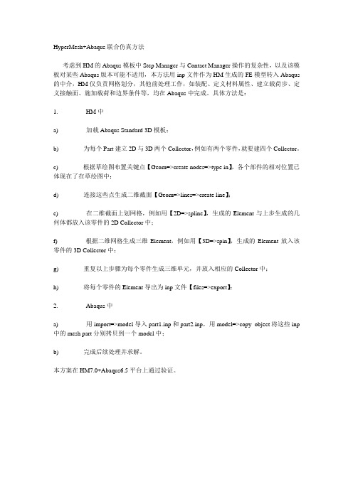
HyperMesh+Abaqus联合仿真方法考虑到HM的Abaqus模板中Step Manager与Contact Manager操作的复杂性,以及该模板对某些Abaqus版本可能不适用,本方法用inp文件作为HM生成的FE模型转入Abaqus 的中介,HM仅负责网格划分,其他前处理工作,如装配、定义材料属性、建立载荷步、定义接触面、施加载荷和边界条件等,均在Abaqus中完成。
具体方法是:1. HM中a) 加载Abaqus Standard 3D模板;b) 为每个Part建立2D与3D两个Collector,例如有两个零件,就要建四个Collector。
c) 根据草绘图布置关键点【Geom=>create nodes=>type in】,各个部件的相对位置已体现在了在草绘图中;d) 连接这些点生成二维截面【Geom=>lines=>create line】;e) 在二维截面上划网格,例如用【2D=>spline】,生成的Element与上步生成的几何体都放入该零件的2D Collector中;f) 根据二维网格生成三维Element,例如用【3D=>spin】,生成的Element放入该零件的3D Collector中;g) 重复以上步骤为每个零件生成三维单元,并放入相应的Collector中;h) 将每个零件的Element导出为inp文件【files=>export】;2. Abaqus中a) 用import=>model导入part1.inp和part2.inp,用model=>copy object将这些inp 中的mesh part分别拷贝到一个model中;b) 完成后续处理并求解。
本方案在HM7.0+Abaqus6.5平台上通过验证。
(完整word版)利用Hypermesh对AbaqusSPH计算的建模方法
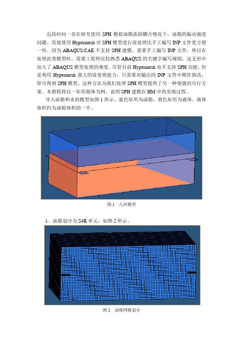
近段时间一直在研究使用SPH模拟油箱流固耦合情况下,油箱的振动强度问题。
发现使用Hypermesh对SPH模型进行前处理比手工编写INP文件更方便一些。
因为ABAQUS/CAE不支持SPH建模,需要手工编写INP文件,所以在处理此类模型时,需要工程师比较熟悉ABAQUS的关键字编写规则,这无形中加大了ABAQUS模型处理的难度。
尽管目前Hypermesh也不支持SPH功能,但是利用Hypermesh强大的前处理能力,只需要对输出的INP文件中稍作修改,即可得到SPH模型。
这种方法为我们处理SPH模型提供了另一种便捷的可行方案。
本教程将以一矩形箱体为例,说明SPH建模在HM中的实现过程。
导入油箱和水的模型如图1所示。
蓝色矩形为油箱,黄色矩形为液体。
液体体积约为油箱体积的一半。
图1 几何模型1、油箱划分为S4R单元,如图2所示。
图2 油箱网格划分2、液体划分为实体单元,如图3所示。
图3 液体网格划分3、生成MASS单元(1)创建新component,命名为water,如图4所示。
图4 component创建面板(2)利用图3液体网格的节点,生成MASS单元,确认其放置在名为water 的component中,如图5~图7所示图5 mass面板图6 生成mass单元图7 放置在water中的MASS单元4、创建材料和属性(1)油箱材料为steel,属性为shell section,厚度为1.0mm。
(2)为water创建材料状态方程,并将材料赋予随后创建的实体截面属性。
图8 进入创建材料面板图9 勾选密度项图10 勾选关键字项图11 液体的材料属性参数图12 为液体创建实体截面属性4、创建相关的接触和分析步后,隐藏图3所示的液体实体单元,导出INP文件,如图13、14所示。
图13 隐藏water_C3D8R图14 以displayed 方式导出INP文件5、打开INP文件,将MASS更改为PC3D,保存,如图15所示。
HyperMesh+Abaqus联合仿真方法
HyperMesh+Abaqus联合仿真方法
考虑到HM的Abaqus模板中StepManager与ContactManager操作的复杂性,以及该模板对某些Abaqus版本可能不适用,本方法用inp文件作为HM 生成的FE模型转入Abaqus的中介,HM仅负责网格划分,其他前处理工作,如装配、定义材料属性、建立载荷步、定义接触面、施加载荷和边界条件等,均在Abaqus中完成。
具体方法是:
1.HM中
a)加载AbaqusStandard 3D模板;
b)为每个Part建立2D与3D两个Collector,例如有两个零件,就要建四个Collector。
c)根据草绘图布置关键点【Geom=>createnodes=>type in】,各个部件的相对位置已体现在了在草绘图中;
d)连接这些点生成二维截面【Geom=>lines=>createline】;
e)在二维截面上划网格,例如用【2D=>spline】,生成的Element与上步生成的几何体都放入该零件的2D Collector中;
f)根据二维网格生成三维Element,例如用【3D=>spin】,生成的Element放入该零件的3D Collector中;
g)重复以上步骤为每个零件生成三维单元,并放入相应的Collector中;
h)将每个零件的Element导出为inp文件【files=>export】;
2.Abaqus中
a)用import=>model导入part1.inp和part2.inp,用model=>copy object将这些inp中的mesh part分别拷贝到一个model中;
b)完成后续处理并求解。
内容整理自网络。
- 1、下载文档前请自行甄别文档内容的完整性,平台不提供额外的编辑、内容补充、找答案等附加服务。
- 2、"仅部分预览"的文档,不可在线预览部分如存在完整性等问题,可反馈申请退款(可完整预览的文档不适用该条件!)。
- 3、如文档侵犯您的权益,请联系客服反馈,我们会尽快为您处理(人工客服工作时间:9:00-18:30)。
6, 接触对的设置
F, 设置接触对
直接选择设好的接触属性和接触面
下面这些接触参数,常用的有adjust、smooth、tie、smallsliding. 如果对这些参数没有理解,可以先不选。
7, 输出设置
A,选择output block 命令
B,在file文件中输出点的位移及约束反力, 单元的应力应变 (U ,RF,SINV ,PE),特殊结果输出参数,参考Abaqus手册。
8, 设置载荷步
A,选择load steps 命令,设置第一个载荷步
B,载荷步的名字应该清楚的说明加载的情况 勾选载荷步包含的载荷(loadcols)及输出设置(outputlocks),点击update
6, 接触对的设置
E, 调整需要添加接触的单元法向相对, 然后添加接触单元
E_1 检查并调整接触网格的单元法向
E_1a
选择单元,显示法向
E_1b
选择法向一致的参考单元
E_1c
调整法向,法向指向接触面
6, 接触对的设置
E, 调整需要添加接触的单元法向相对, 然后添加接触单元 E_2 添加接触单元到主从接触面
2, 材料建立
A,选ity,输入材料密度。注意:单位制(吨t,毫米mm,牛N,兆帕MPa,秒S)
C,勾选Elastic,输入材料线性属性,弹性模量E,及泊松比NU
试验应力应变曲线值需要 转换成材料的真实应力-塑 性应变曲线。 转换公式参考相关资料。 下面的文件包含转换模板。
OP=MOD,表示保留上一步设置 OP=NEW,表示不保留上一步设置
程序默认值是OP=MOD
8, 设置载荷步
D,第二个载荷步的设置
跟第一个载荷步的设置一样,唯一需要理解的是Load_OP 参数的选择
下面的例子是第二步卸载unloading
程序默认延续第一步的输出设置 、边界条件、加载条件。 所以如果输出没有改变,就不用在第二步设置输出,也不用重新设置约束 条件,只需要改变加载条件
9, 检查模型
A,检查component厚度和重量是否正常
B,检查连接,使用F5-elment-by attached 。
看是否存在没有连接的component,如果有,这些没有连接的component是否已经约束,如果也 没有约束,模型就不会收敛,需要用弹簧单元弱连接到相邻的零件上。
C,检查加载及约束,先输出inp文件 。查找关键字*step,查看每个 step的 载荷、约束及输出是否正常,有没有漏选约束条件。
hypermesh与Abaqus联合仿真经典教程
1,检查网格,规范网格component命名 2,建立材料 3,建立component属性props,不同材料相同厚度要分开建立
(hypermesh8不需要单独建立props,直接在 component参数中写厚度,选材料)
4,零件连接 5,设置约束及加载 6,设置接触 7,设置输出参数 8,设置载荷步(load step) 9,检查模型 10,输出debug
C-2,Analysis Procedure 选择
静力分析选择Static, 然后勾选Dataline。 模态分析选择Frequency
初始步长
最小步长 最大步长
C-3,Load_OP 选择
Load_OP用来设置是否需要保留上一步 的边界条件(Boundary)或者是载荷(集 中载荷Cload 、面载荷Dload)
10, 输出DEBUG
ljtleon 第一版 2009年12月8日
1、 命名规范
任何名字都不能有特殊符号,尽量只包含字母、数字、中划线和下划线, 任何名字都不能用数字开头,只能用字母开头。 经常出错的是数字中的“点”号,用字母p代替。 Component 命名规范
零件名字或者编号_厚度_材料名字_顺序编号 (只用于前面都相同的情况) 名字太长时,可以简写。
4, 焊点,单元类型是1D/rigid/Beam
选择多点方式 连接焊点位置上下各一个单元的点,连接完成后,显示BEAM 单元类型
4, 焊点,一维单元类型转换1D/config edit
现在模型里面用的是单点连接,也行,但是单元类型spring不对,需要转换成Beam。 选择config edit命令
A,选择要转换的单元
B,选择新单元类型rigid
C,转换
5, 边界条件及载荷设置
A, 建立约束loadcol
B, 设置约束
C, 建立加载 loadcol ,加载力或者通过约束加强迫位移
不同的载荷及约束条件要放在不同的loadcol里,方便后续设load step时选用
加载集中力 强迫位移X 方向10mm
6, 接触对的设置
A,建立主接触面,注意命名,名字后面加上_M B,建立从接触面,注意命名,名字后面加上_S C,建立接触对,注意命名,名字后面加上_P,类型选 contact_pair D,建立接触属性
D_1 打开属性面板
6, 接触对的设置
D_2 建立接触属性,注意接触类型的选择
D_3 设置接触摩擦系数参数,先要勾选Friction, 在没有数值的情况下,可 以用0.2作为默认值,
C ,点击edit ,进入载荷步参数设置页面
8, 设置载荷步
C-1,step parameter 选择
一般选increment =500,设置总的迭代步数,默认是100, 有时候如果模型接触太多,可能100步不够。
另外可以勾选Nlgeom,如果模型本身包含了非线性的设 置(非线性材料,设置接触等),程序默认选择Nlgeom。
D,勾选Plastic,输入材料非线性属性:真实应力_塑性应变曲线
这里填入的是3点材料,包含 第一点,屈服应力。 第二点,极限应力应变。 第三点,延伸应力应变,应力比极限应力稍大一点,但是应 变很大,这样保持延伸应力应变曲线平直,模拟材料破坏。
3, 刚性网格的属性
只需要选择 A,刚性网格的参考点,(参考点可以设在加力点上) B,刚性网格的component 注意:刚性网格的单元类型要更新成R3D3、R3D4,普通单元类型是S3、S4。 命令是2D/elem types