将PSCAD中的数据导入MATLAB
关于matlab及pscad中abc2dq模块的使用
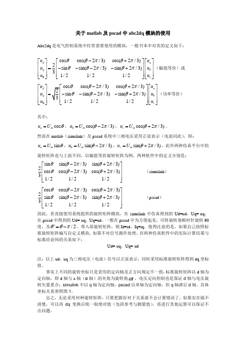
关于matlab 及pscad 中abc2dq 模块的使用Abc2dq 是电气控制系统中经常需要使用的模块,一般书本中对其的定义如下:0cos cos(2/3)cos(2/3)2sin sin(2/3)sin(2/3)31/21/21/2d a q b c u u u u u u θθπθπθθπθπ-+⎡⎤⎡⎤⎡⎤⎢⎥⎢⎥⎢⎥=----+⎢⎥⎢⎥⎢⎥⎢⎥⎢⎥⎢⎥⎣⎦⎣⎦⎣⎦(幅值等价)或0cos cos(2/3)cos(2/3)2sin sin(2/3)sin(2/3)31/21/21/2d a q b c u u u u u u θθπθπθθπθπ-+⎡⎤⎡⎤⎡⎤⎢⎥⎢⎥⎢⎥=----+⎢⎥⎢⎥⎢⎥⎢⎥⎢⎥⎢⎥⎣⎦⎣⎦⎣⎦(功率等价)其中:cos a m u U θ=,cos(2/3)b m u U θπ=-,cos(2/3)c m u U θπ=+。
然而在matlab (simulink )及pscad 系统中三相电压采用正弦表示(电流同此),即:sin a m u U θ=,sin(2/3)b m u U θπ=-,sin(2/3)c m u U θπ=+,此外两种仿真平台中的旋转矩阵也与上面不同,以幅值等价旋转矩阵为例,两种软件中的定义分别是:sin sin(2/3)sin(2/3)2cos cos(2/3)cos(2/3)31/21/21/2θθπθπθθπθπ-+⎡⎤⎢⎥-+⎢⎥⎢⎥⎣⎦ (simulink )cos cos(2/3)cos(2/3)2sin sin(2/3)sin(2/3)31/21/21/2θθπθπθθπθπ-+⎡⎤⎢⎥-+⎢⎥⎢⎥⎣⎦(pscad )因此,若直接使用系统提供的旋转矩阵模块,在simulink 中仿真得到的Ud=ud ,Uq=-uq ,在pscad 中得到的Ud=-uq ,Uq=ud 。
一般在pscad 中为方便起见,可将旋转角顺时针旋转90度,及'/2θθπ=-,带入原旋转矩阵,则Id=id ,Iq=iq 。
CAD文件的数据导入和导出技巧
CAD文件的数据导入和导出技巧以CAD文件的数据导入和导出技巧为题,以下是一篇1500字左右的高质量文章。
CAD文件是计算机辅助设计的常用文件格式,广泛应用于工程设计、建筑设计、电子设计等领域。
在设计过程中,常常需要将CAD文件导入到其他软件中进行进一步的处理,或者将其他软件中的数据导入到CAD软件中进行设计。
本文将介绍一些CAD文件的数据导入和导出技巧,帮助读者更好地应用CAD软件。
一、CAD文件的数据导入1. 导入常见文件格式CAD软件通常支持导入多种常见文件格式,如DXF、DWG、STEP、IGES等。
在导入时,需要注意选择正确的文件格式,并根据需要设置导入选项,如单位、文件精度等。
此外,还可以根据文件内容的不同选择合适的导入模式,如导入构件、导入点等。
2. 提前准备工作在将CAD文件导入到其他软件中之前,有时需要进行一些提前准备工作。
例如,如果导入的CAD文件中有字体或材质文件,在导入前应确认其在其他软件中是否可用,需要事先安装字体或导入材质文件。
此外,还应对CAD文件进行简化处理,删除不必要的元素,以减小导入的数据量。
3. 校验导入结果导入CAD文件后,应仔细校验导入结果,确保导入的数据与原始CAD文件保持一致。
可以逐个比对导入结果中的元素,如线条、曲线、面片等,确认其位置、形状、属性等是否正确。
如发现问题,可以尝试重新导入或调整导入选项,以获得更好的导入结果。
二、CAD文件的数据导出1. 导出常见文件格式与导入相类似,CAD软件也支持导出多种常见文件格式。
在导出时,同样需要选择正确的文件格式,并根据需要设置导出选项,如单位、文件精度等。
此外,还可以选择导出的CAD元素,如线条、曲线、面片等,以满足导出文件的需求。
2. 导出前数据清理在将CAD文件导出到其他软件中之前,应进行一些数据清理工作。
首先,应删除不需要导出的元素,减小导出文件的数据量。
其次,应检查导出文件中的线段、曲线是否光滑,面片是否封闭,确保导出的数据符合其他软件的要求。
MATLAB导入CAD数据
|—用AutoCAD绘制平面公式曲线(如渐开线、心形线)、空间公式曲线(如螺旋线)以及公式曲面(如马鞍形曲面)是比较困难的,一般情况下,需要用AutoCAD开发程序编程,但多数程序比较复杂,尤其是公式曲面的绘制程序,需要多层嵌套循环,复杂且运行效率低。
快速且精确地绘制各种公式曲线、曲面恰恰是MATLAB勺长项,但是MATLAB^制的图形却不能直接用于机械零件设计。
其中非常关键的一点,就是MATLAB绘制的曲线、曲面分别是由有限个点连接而成的折线和空间网格构成的,而在AutoCAD中绘制的曲线、曲面也是如此。
因此,只需要把在MATLAB^绘制的公式曲线、曲面上所有的点坐标数据都提取出来,若能让AutoCAD正确识别,那么我们就可以在AutoCAD中精确地绘制这些曲线、曲面了。
本文介绍了一种快速、精确地绘制各种公式曲线、曲面的方法,即在AutoCAD中通过调用经过Excel处理的MATLAB数据实现。
二、AutoCAD和MATLAB勺特点MATLAB!非常优秀的科学计算、信号处理以及图形显示软件,它有自身的语言,与其他高级语言相比,MATLAB供了一个人机交互的数学环境,并以矩阵作为基本的数据结构,可大大节省编程时间。
另外,MATLA环仅语法规则简单,容易掌握,调试方便,还可以存储中间结果,这使得MATLAB既可以快捷、精确地绘制各种公式曲线、曲面,又可以很方便地提取中间数据。
在工业设计领域,AutoCAD不仅被广泛应用于平面绘图,也可以用于三维建模,但在曲线、曲面造型方面不是很理想。
它是开放型的人机交互系统,有多种语言接口,与外界的数据交换很灵活,这些特点使得它与MATLAB勺结合成为可能。
三、结合MATLAB在AutoCAD中绘制曲线、曲面的原理及方法1. 原理MATLAB^的矩阵数据虽然很容易提取,但由于它不是AutoCAD能识别的格式,因此不能直接被AutoCAD调用,需要先用Excel对从MATLAB中提取的数据进行编辑,转换成Aut oCAD可以识别的格式,才能在AutoCAD中绘出曲线、曲面。
PSCAD模块库功能教程(包含与matlab接口)
本组件主要用来将选择好的仿真时间步长分派给数据信号线或组件的输入。 它的输 出会随着工程设定的仿真时间步长的变化而自动调整。
9. Time Signal Variable(时间信号变量)
本组今年主要用来将选择好的仿真时间分派给数据信号线或组件的输入。 它的输出 会随着工程设定的仿真时间步长的变化而自动调整。
11. Total Number of Multiple Runs (多路运行的总数)
本组件专用于 PSCAD 的 “Multiple Run” 特性, 给出多路运行的总数, “Multiple Run” 特性可以在工程属性窗口中旋转“可用”或“不可用”。此值可用于“Multiple Run”研 究的组件和控制系统的直接输入。 此组件可以和 “Current Run Number” 组件一起使用。
PSCAD 中不同类型的数据介绍
1. Real Constant(实常数)
本组件主要用来给数据线或者组件输入分配一个实数型常数。
2. Integer Constant(整数型常数)
本组件主要用来给数据线或者组件输入分配一个整数型常数。
3. Logical Constant(逻辑型常数)
本组件主要用来给数据线或者组件输入分配一个逻辑型常数。.TRUE.和.FALSE.可 通过选择 True 和 False 直接指定。其它的选项包括:
2 = 1.414213562373095
3 = 1.732050807568877 1/ 2 = 0.707106781186548 1/ 3 = 0.577350269189626
1/3 = 0.333333333333333 2/3 = 0.666666666666667
5. Type Conversion(类型转换)
CAD中的数据导入与引用技巧与实例
CAD中的数据导入与引用技巧与实例CAD软件是设计领域中广泛使用的工具,它能够帮助用户创建和编辑各种图形,而数据导入和引用是CAD软件中常用的功能。
本文将介绍CAD中的数据导入和引用的技巧,并通过实例演示其操作方法。
一、数据导入技巧1. 使用插入命令导入外部文件:CAD软件可以插入多种不同格式的文件,如图像、PDF、Excel、Word等。
只需在绘图空间中使用“插入”命令,选择要导入的文件即可。
插入后的文件会以一个单独的对象显示在绘图中,可以随意移动和缩放。
2. 从其他CAD文件中导入:如果需要将另一个CAD文件中的图形导入到当前绘图中,可以使用“插入”命令,并选择要导入的CAD文件。
导入后的图形将作为一个块对象显示在绘图中,可以随意移动和缩放。
3. 导入外部图形作为参考:在一些情况下,我们可能只需要将外部图形作为参考,在绘图中进行修改或测量。
这时可以使用“Xref”命令将外部图形导入到当前绘图中,作为一个外部参考。
可以选择是否锁定和显示该外部参考,并可以通过更改外部参考的路径来更新图形。
二、数据引用技巧1. 使用块引用:块是CAD中的一种组合对象,可以包含多个图形元素。
通过创建块对象并在多个地方引用,可以节省大量的绘图时间。
使用“创建块”命令将选定的图形元素组合为一个块对象,并为该块对象命名。
然后使用“块引用”命令将该块对象引用到绘图中的其他位置,可以通过更改块对象的定义来同时修改所有引用。
2. 使用外部图形引用:如果需要在当前绘图中引用其他CAD文件中的图形,可以使用“Xref”命令。
选择要引用的CAD文件并设置相关选项(如路径、缩放比例等),确定后图形将作为一个外部引用显示在当前绘图中,可以随意移动和缩放。
与块引用不同,外部引用不可编辑,但可以通过更改外部引用的路径来更新图形。
3. 使用图像引用:有时我们可能需要在CAD绘图中引用图片,如地图、照片等。
可以使用“插入”命令选择要引用的图像文件,并设置相关选项(如缩放比例、插入点等)。
CAD中的数据导入和导出方法

CAD中的数据导入和导出方法在使用CAD软件时,有时我们需要将数据从其他软件导入到CAD中或将CAD中的数据导出到其他软件中。
这些操作对于数据交换和协作非常重要。
在本篇文章中,我们将讨论CAD中的数据导入和导出方法。
首先,我们来讨论从其他软件导入数据到CAD中的方法。
CAD软件通常支持导入各种格式的数据,例如DXF、DWG、IGES、STEP等。
要实现从其他软件导入数据,我们可以打开CAD软件并选择文件菜单中的“导入”选项。
然后,我们需要选择要导入的文件格式,并浏览到相应的文件路径。
最后,单击导入按钮即可将数据导入到CAD中。
在导入过程中,可能需要进行一些配置和调整以确保数据正确解析和转换。
一旦导入完成,我们就可以在CAD中查看和编辑导入的数据了。
除了导入数据到CAD中外,我们有时还需要将CAD中的数据导出到其他软件中。
同样地,CAD软件也支持导出各种格式的数据。
要实现从CAD导出数据,我们可以选择文件菜单中的“导出”选项。
然后,我们需要选择要导出的文件格式,并为导出文件指定路径和名称。
最后,单击导出按钮即可将CAD中的数据导出到指定的文件中。
导出过程中可能需要进行一些配置和调整,以确保导出的数据格式和内容符合我们的需求。
一旦导出完成,我们就可以将数据在其他软件中打开和使用了。
在CAD中,除了导入和导出整个文件的数据,我们还可以选择性地导入和导出特定的图形元素和图层。
例如,当我们从其他软件导入数据时,可以选择只导入某些特定图层的内容,从而减少导入的复杂性和数据量。
同样地,在导出数据时,我们也可以选择只导出某些图层或图形元素,以满足特定需求。
这种选择性导入和导出的功能在协作和数据交换中非常有用。
此外,CAD软件通常还支持数据格式的转换和转换。
例如,在CAD软件中,我们可以将DWG格式的文件转换为DXF格式,或将DWG/DXF格式的文件转换为IGES或STEP格式。
这些转换功能可以帮助我们在不同的CAD软件之间实现数据的无缝转换和交流。
用Scopeview处理pscad波形数据得到Matlab数据格式
步骤
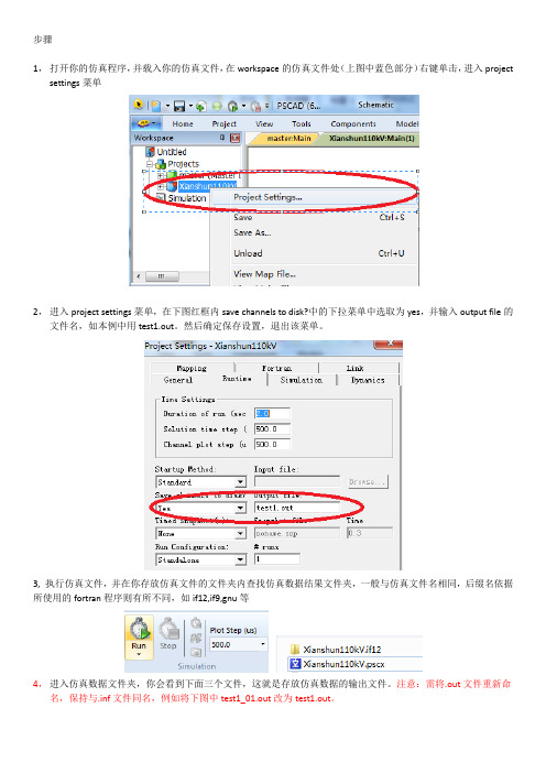
1,打开你的仿真程序,并载入你的仿真文件,在workspace的仿真文件处(上图中蓝色部分)右键单击,进入project settings菜单
2,进入project settings菜单,在下图红框内save channels to disk?中的下拉菜单中选取为yes,并输入output file的文件名,如本例中用test1.out。
然后确定保存设置,退出该菜单。
3, 执行仿真文件,并在你存放仿真文件的文件夹内查找仿真数据结果文件夹,一般与仿真文件名相同,后缀名依据所使用的fortran程序则有所不同,如if12,if9,gnu等
4,进入仿真数据文件夹,你会看到下面三个文件,这就是存放仿真数据的输出文件。
注意:需将.out文件重新命名,保持与.inf文件同名,例如将下图中test1_01.out改为test1.out。
5,打开scopeview数据处理软件,会出现两个窗口,其中1号窗口是波形显示窗口,2号窗口是信号选择窗口。
在2号窗口中单击3号方框内的打开文件按钮。
5,将出现下面数据源选择窗口,将文件类型选为pscad files,然后进入第3步中的数据文件夹中,找到第4步中的test1.inf文件,选取并单击Load按钮。
6,出现类似下面的窗口,选取你所需要的信号,如本图中选取了两个actloss和IH1.,然后单击红框内的按钮。
输出结果如下图所示。
6,如要保存为其他数据格式,如Matlab数据,则按照下图,先单击1中的按钮,然后在2处输入保存文件名,最后单击export按钮,本例中输出到123.mat文件。
7,双击mat文件可看到如下matlab软件窗口,可以看到actloss和IH1所有数据均已经保存。
Matlab数据导入方法
Matlab数据导入方法在编写一个程序时,经常需要从外部读入数据,或者将程序运行的结果保存为文件。
MATLAB使用多种格式打开和保存数据。
本章将要介绍 MATLAB中文件的读写和数据的导入导出。
13.1 数据基本操作本节介绍基本的数据操作,包括工作区的保存、导入和文件打开。
13.1.1 文件的存储MATLAB支持工作区的保存。
用户可以将工作区或工作区中的变量以文件的形式保存,以备在需要时再次导入。
保存工作区可以通过菜单进行,也可以通过命令窗口进行。
1. 保存整个工作区选择File菜单中的Save Workspace As…命令,或者单击工作区浏览器工具栏中的Save,可以将工作区中的变量保存为MAT文件。
2. 保存工作区中的变量在工作区浏览器中,右击需要保存的变量名,选择Save A s…,将该变量保存为MAT文件。
3. 利用save命令保存该命令可以保存工作区,或工作区中任何指定文件。
该命令的调用格式如下:● save:将工作区中的所有变量保存在当前工作区中的文件中,文件名为matlab.mat,MAT文件可以通过load函数再次导入工作区,MAT函数可以被不同的机器导入,甚至可以通过其他的程序调用。
● save('filename'):将工作区中的所有变量保存为文件,文件名由filename 指定。
如果filename中包含路径,则将文件保存在相应目录下,否则默认路径为当前路径。
● save('filename', 'var1', 'var2', ...):保存指定的变量在 filename 指定的文件中。
● save('filename', '-struct', 's'):保存结构体s中全部域作为单独的变量。
● save('filename', '-struct', 's', 'f1', 'f2', ...):保存结构体s中的指定变量。
将CAD的史都华平台转换到Matlab中(Translating a CAD Stewart Platform)
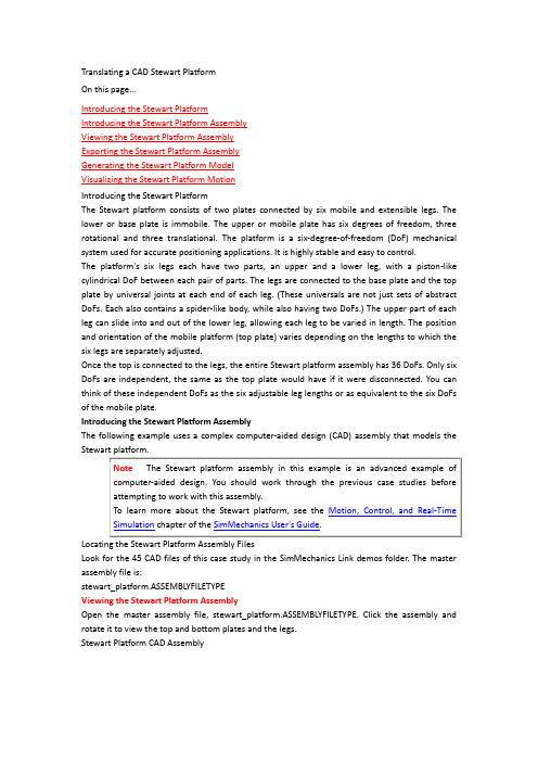
Translating a CAD Stewart PlatformOn this page…Introducing the Stewart PlatformIntroducing the Stewart Platform AssemblyViewing the Stewart Platform AssemblyExporting the Stewart Platform AssemblyGenerating the Stewart Platform ModelVisualizing the Stewart Platform MotionIntroducing the Stewart PlatformThe Stewart platform consists of two plates connected by six mobile and extensible legs. The lower or base plate is immobile. The upper or mobile plate has six degrees of freedom, three rotational and three translational. The platform is a six-degree-of-freedom (DoF) mechanical system used for accurate positioning applications. It is highly stable and easy to control.The platform's six legs each have two parts, an upper and a lower leg, with a piston-like cylindrical DoF between each pair of parts. The legs are connected to the base plate and the top plate by universal joints at each end of each leg. (These universals are not just sets of abstract DoFs. Each also contains a spider-like body, while also having two DoFs.) The upper part of each leg can slide into and out of the lower leg, allowing each leg to be varied in length. The position and orientation of the mobile platform (top plate) varies depending on the lengths to which the six legs are separately adjusted.Once the top is connected to the legs, the entire Stewart platform assembly has 36 DoFs. Only six DoFs are independent, the same as the top plate would have if it were disconnected. You can think of these independent DoFs as the six adjustable leg lengths or as equivalent to the six DoFs of the mobile plate.Introducing the Stewart Platform AssemblyThe following example uses a complex computer-aided design (CAD) assembly that models theLocating the Stewart Platform Assembly FilesLook for the 45 CAD files of this case study in the SimMechanics Link demos folder. The master assembly file is:stewart_platform.ASSEMBLYFILETYPEViewing the Stewart Platform AssemblyOpen the master assembly file, stewart_platform.ASSEMBLYFILETYPE. Click the assembly and rotate it to view the top and bottom plates and the legs.Stewart Platform CAD AssemblyThe CAD hierarchy for the Stewart platform contains assemblies for the top and base plates, as well as assemblies for the six legs. All the constraints on the assembly parts are grouped into one group, containing 30 constraints. There are 448 component parts and 38 subassemblies, which you can open individually to examine the separate parts.The base plate is about 24 centimeters (cm) in diameter; the top plate about 16.5 cm. When centered and oriented flat, the top plate is about 20 cm above the base. The assembly models the platform material as aluminum (about 2.7 grams per cubic cm).Exporting the Stewart Platform AssemblyApply any changes you want to the assembly configuration or settings. If you change the assembly or any subassemblies, you need to rebuild the assembly before exporting it to XML. Using the SimMechanics Link interface to your CAD platform, export the assembly into Physical Modeling XML. Because the assembly is so complex, the export process takes longer than it does for simpler assemblies. As the export proceeds, various parts and subassemblies are highlighted. When the highlighting stops, the export is finished.The exported model appears as stewart_platform.xml in your working CAD folder.Generating the Stewart Platform ModelMove or copy the stewart_platform.xml file into your working MATLAB folder.To generate a new Simulink model, enter mech_import('stewart_platform') at the MATLAB command line, and wait for the model generation stewart_platform to finish.Inspecting the Generated Model and Counting Its DoFsThe complete Stewart platform model contains seven subsystems.Stewart Platform Model: Base, Legs, and Top PlateThe subsystems correspond to the subassemblies of the original CAD assembly — the base plate and the six platform legs.The base plate subassembly BaseRingAssembly-1 contains six subassemblies, modeling a base swivel bearing for each leg.The six leg subassemblies, ActuatorAssm, model the upper and lower halves of each leg and represent part of their DoFs.For each leg, there are six DoFs. Two pairs of revolutes associated with each leg represent the two universal joints connecting each leg to the top and base plates, respectively. Each of these universals has two DoFs.At the top level, there are two revolutes, one attached to either end of a leg subassembly,connecting each leg to the base and top plates, respectively.Within each leg subassembly, there are two other revolutes, each one connecting the leg to the top and base plates, respectively.One of the revolutes inside the leg subassembly pairs with one of the revolutes outside the leg assembly to make up a two-DoF universal. These pairs occur twice on each leg, one connecting the leg to the top plate, the other connecting the leg to the base plate.Within each leg subassembly, there is one prismatic, representing the leg's freedom to expand or contract along its shaft.Within each swivel bearing subassembly, itself located within the base ring assembly, is another revolute representing each leg's freedom to rotate about its shaft.Each leg has six DoFs. However, the constraints imposed by attaching each leg to fixed points on the base and top plates, respectively, reduce these to one independent DoF for each leg — the freedom to expand or contract along its shaft.The rotational DoFs associated with the universals at the attachment points are completely dependent on the leg's prismatic DoF.The rotational DoFs associated with the cylindricals in each leg are completely dependent on the universals at the top and bottom of each leg.Deleting Unnecessary Bodies and JointsThe generated model contains a large number of redundant Root Weld and zero-mass Root Part blocks. You can delete these and not affect the model's dynamics, as long as you take care to reconnect the remaining bodies properly after deleting each Weld.Adding Actuators and SensorsIf you want the motion of the platform to be controlled by something other than gravity, you need to add the appropriate Actuators to the model. To quantify the model's motion, you need to make precise measurements with Sensors. You can drive the actuators with external control signals to model an open-loop controller for the Stewart platform. If you introduce feedback from the sensors to the actuators, you can model a closed-loop controller.weight. You can verify this by running and visualizing your Stewart platform model.From the Simulation menu, select Configuration Parameters. The Configuration Parameters dialog opens. Choose the SimMechanics node.Select Display machines after updating diagram and Show animation during simulation. Click Apply or OK.From the Edit menu, select Update Diagram. The SimMechanics visualization window opens with the SimMechanics controls. The window displays the Stewart platform in its initial position. Start the simulation by clicking the Start button in the toolbar of either the visualization window or the model window.The mobile plate falls under its own weight and reaches the base plate in about 0.2 seconds. Because there is nothing to stop the legs or the top plate, the platform continues to collapse: the mobile plate falls below the base plate, and the upper and lower parts of each leg come apart. This visualization of the Stewart platform uses custom body visualization with the STL body geometry files exported from the original CAD assembly.SimMechanics Visualization of the CAD-Based Stewart Platform (Custom Body Geometries)Viewing a Stewart Platform AnimationIf you are connected to the Internet, have an AVI-compatible media streaming application installed on your system, and want to play a recorded animation of this system:Click the following link. When the download dialog opens, choose Save to file and specify a file name and location on your system.Click OK to save the AVI file to your system.Once the downloading is complete, start the AVI animation on your system.If you do not have an AVI-compatible application, consider using the MATLAB VideoReader class and its read method instead.This is a compressed AVI recording, which requires that you have the Indeo 5 video codec installed to decompress and play.Download animationThe animation shows the Stewart platform moving through a predefined trajectory, as simulated by the mech_stewart_trajectory demo. For clarity, the animation displays the convex hulls, a surface for the top plate, and lines for the legs. The animation steps through the predefined SimMechanics viewpoints to show different perspectives on the moving platform.。
CAD数据导入与导出技巧与其他软件的无缝交互
CAD数据导入与导出技巧与其他软件的无缝交互1.选择正确的文件格式:不同的CAD软件支持不同的文件格式,如DWG、DXF、STL、IGES等。
在导入或导出CAD数据之前,确保选择正确的文件格式,以确保数据的准确性和完整性。
2.导入和导出选项的优化:CAD软件通常提供了许多导入和导出选项,可以调整导入和导出的精度、比例、层次结构等。
根据需要,对这些选项进行优化,以获得最佳的导入和导出结果。
3.使用中间文件格式:如果两个CAD软件不直接支持相同的文件格式,可以使用中间文件格式进行数据传输,如将DWG文件导出为DXF文件,然后将DXF文件导入到另一个CAD软件中。
尽量避免使用不受支持的文件格式进行导入和导出,以防止数据损坏和丢失。
4. 使用插件和转换工具:许多CAD软件提供了插件和转换工具,可以帮助实现CAD数据的无缝交互。
例如,AutoCAD提供了多个插件和工具,可以将CAD数据导入和导出到其他软件,如Revit、Inventor等。
使用这些插件和工具可以极大地简化数据传输和共享的过程。
5.共享CAD数据:除了导入和导出CAD数据之外,还可以考虑使用云存储和协作平台来共享CAD数据。
通过将CAD数据上传到云端,可以方便地与其他团队成员进行共享和协作,无需进行繁琐的导入和导出操作。
7.准备工作:在导入和导出CAD数据之前,进行必要的准备工作非常重要。
检查数据的完整性和准确性,并确保数据的单位和比例尺与目标软件环境相匹配。
清理和修复CAD数据中存在的任何错误和问题,以确保无缝交互。
总的来说,CAD数据的导入和导出是CAD软件中非常重要的功能之一、通过选择正确的文件格式、优化导入和导出选项、使用插件和转换工具、共享CAD数据、更新和同步数据以及进行必要的准备工作,可以实现CAD数据与其他软件之间的无缝交互,并确保数据的准确性和完整性。
matlab中的数据导入和导出
Matlab文件和数据的导入与导出Matlab文件和数据的导入与导出在编写一个程序时,经常需要从外部读入数据,或者将程序运行的结果保存为文件。
MATLAB使用多种格式打开和保存数据。
本章将要介绍MATLAB中文件的读写和数据的导入导出。
13.1 数据基本操作本节介绍基本的数据操作,包括工作区的保存、导入和文件打开。
13.1.1 文件的存储MATLAB支持工作区的保存。
用户可以将工作区或工作区中的变量以文件的形式保存,以备在需要时再次导入。
保存工作区可以通过菜单进行,也可以通过命令窗口进行。
1. 保存整个工作区选择File菜单中的Save Workspace As…命令,或者单击工作区浏览器工具栏中的Save,可以将工作区中的变量保存为MAT文件。
2. 保存工作区中的变量在工作区浏览器中,右击需要保存的变量名,选择Save As…,将该变量保存为MAT文件。
3. 利用save命令保存该命令可以保存工作区,或工作区中任何指定文件。
该命令的调用格式如下:● save:将工作区中的所有变量保存在当前工作区中的文件中,文件名为matlab.mat,MAT文件可以通过load函数再次导入工作区,MAT函数可以被不同的机器导入,甚至可以通过其他的程序调用。
● save('filename'):将工作区中的所有变量保存为文件,文件名由filename指定。
如果filename中包含路径,则将文件保存在相应目录下,否则默认路径为当前路径。
● save('filename', 'var1', 'var2', ...):保存指定的变量在filename 指定的文件中。
● save('filename', '-struct', 's'):保存结构体s中全部域作为单独的变量。
● save('filename', '-struct', 's', 'f1', 'f2', ...):保存结构体s中的指定变量。
利用Matlab对Excel数据表参数进行频谱分析(FFT)的方法
方法
1.打开matlab ,导入pscad生成的.out格式的数据文件。
2.创建一个simulink仿真模型,调出“powergui”和示波器“scope”。
点击进入scope,在‘Configuration Propeties’的Logging中,选中log data to workspace,创建变量名(自定义,例如Current)和保存形式(设为Structure With Time)。
保存simulink文件,并仿真一次。
3.仿真之后,就会在工作区生成一个变量ScopeData。
在命令行窗口输入:
ScopeData.time = a; %将a向量赋给Current时间坐标轴
ScopeData.signals.values = b; %将b向量赋给Current信号值坐标
power_fftscope %调用Powergui FFT Analysis Tool 4.弹出FFT的GUI窗口,在Available signals项下,选择要分析的信号name(即
Current),GUI会绘制出信号波形和频谱图,点击相应按钮,可以设置需要进行FFT分析的信号起始时间、周期数等,非常直观。
实质上,这种方法是利用了Powergui分析simulink示波器输出信号的FFT工具。
将AutoCAD图形导入常用软件
一、在Word文档中插入AutoCAD图形Word绘图功能有限,一旦遇到较复杂的图形,只能“望图兴叹”。
AutoCAD是专业绘图软件,功能强大,很适合绘制比较复杂的图形,用AutoCAD绘制好图形,然后插入Word 制作就能解决问题。
插入方法:①用AutoCAD提供的Export功能先将AutocAD图形以BMP或WMF等格式输出,然后插入Word文档②把AutoCAD图形拷贝到剪贴板,再在Word文档中粘贴。
需要注意的是,由于AutoCAD 默认背景颜色为黑色,而Word背景颜色为白色,所以事先把AutoCAD图形背景颜色改成白色,使用菜单命令“工具→系统配置”,在弹出的对话框中选中Display标签,单击color按钮,弹出一对话框,在其中将屏幕作图区的颜色改为白色(即R=G=B=255)后,按下确定按钮,注意此时屏幕作图区的底色变为白色。
另外,AutoCAD图形插入Word文档后,往往空边过大,效果不理想。
利用Word图片工具栏上的裁剪功能进行修整,空边过大问题即可解决。
这个方法既可用于Word也可用以微软Office系列的其它软件,如PowerPint、Excel等二、将AutoCAD导入FlashFlash中有很多“绘图”工具,而且能做出令人心跳的动画,但如果需要输入更复杂一些的图片,如机械装配图、零件图与建筑效果等图片,Flash就无能为力了。
这时我们可以插入AutoCAD提供的图片,在Flash中插入AutoCAD图形的方法如下:<br/><br/><img src=/Upload/2005-12/03702t01.jpg><br/>首先在AutoCAD中将画好的图形保存为*.dxf类型的文件(如图)。
然后在Flash中单击[文件]→[导入]菜单。
在弹出的“导入”对话框中选择文件类型为“AutoCAD DXF (*.dxf)”,输入文件名,单击[打开]按钮。
将PSCAD中的数据导入MATLAB
如何将PSCAD/EMTDC中的数据导入MATLAB中呢?以接地极线路单线接地故障(将模型命名为WLDanjiedi01)为例进行详细的介绍:1、模型建立完毕,右击选择“Project Settings”出现如下界面将”Save channels to disk?”选择为“Yes”,并在后面的“Output file”进行输出文件的命名,如例文件名命名为“WLDanjiedi01.out”(最好与模型名称一致),将模型保存至XX位置。
2、模型仿真完毕,在XX位置会生成一个名为“WLDanjiedi01.emt”的文件夹,文件夹中后缀为“WLDanjiedi01-01.out到WLDanjiedi01-06.out”的文件储存着仿真所得到的数据;名为“WLDanjiedi01.inf”的文件是所有数据的说明,如果需要在MATLAB中进行编程处理数据,则要根据此文件中的说明在MATLAB中进行变量的定义。
3、在MATLAB中的工作窗口如下,单击“Import data”找到“WLDanjiedi01.emt”目录,界面如下下拉文件类型(T)选择“All Files(*.*)”出现如下界面选择“WLDanjiedi01-01.out到WLDanjiedi01-06.out”中所需要的即可,例如导入“WLDanjiedi01-01.out”,选中后点击打开,经过一定时间会出现如下界面选择“Next”,接着选择“Finish”即可完成数据的导入,此时MATLAB中的工作窗口如下,出现了“WLDanjiedi01-01”文件夹。
选中“WLDanjiedi01-01”,界面变成如下,单击“Plot(WLDanjiedi01-01)”会生成此文件夹所包含数据的波形图。
双击“WLDanjiedi01-01”出现如下界面随便选中某一列然后点击上方的“Plot(WLDanjiedi01-01)”即可生成此列所表示的数据波形图。
matlab建模数据的导入与导出

五Hale Waihona Puke 数据导出• save filename varlist 文件格式为mat,只能用load filename 导入 • dlmwrite(„filename‟,m):writes matrix m into filename using the “,” as the delimiter. 可用 dlmread(„filename‟) 或csvread(„filename‟) 读取 • csvwrite(filename,m) writes matrix m into filename as comma separated values. 结果与dlmwrite相同
七、图形的复制与保存
• 图形窗口->edit->copy figure-> word文档->粘贴
努力不一定成功 放弃一定是失败
处理函数 数值文件(一般分隔):dlmread, dlmwrite ,load ,save 文本文件(逗号分隔) :textread, csvread, csvwrite 二进制文件:fopen, fread, fwrite, fclose 格式化的文本输入/输出:fscanf, fprintf 图像数据的读写:imread, imwrite,imshow
其中names、 types 、 answer 均为cell数据类型。如 names{1} 对应‘Sally‟ answer{2}对应‘No‟。 x, y 均为double型 数组
• • • •
2009年全国数模赛B题数据的 导入
题目: 第一步:现将数据复制到记事本中: 第二步:编写程序,读取数据 第三部:数据处理与分析
• 学好计算机的唯一途径是
• 你的编程能力与你在计算机上练习编程 所投入的时间成
使PSpice输出数据文件可以导入到MATLAB中绘制图形
8
图 1 - 2 ice 仿真数据的 Matlab 可视化
将 MATLAB 中的图形数据与 no.8.out 文件中的数据一一对照 两组数据完全一致 知 ps2m1.m 能正确读入文本文件中包含的按列纪录的数据
故可
例二 本例说明如何将一个.Probe 数据存为 文本文件 在将文件中的数据和它们的 名称读入 MATLAB 进而可以推广到一般
PDF created with pdfFactory Pro trial version
图 1 - 1 Pspice 仿真数据的 PROBE 可视化
编写 ps2m1.m 文件 其中读入数据部与绘图部分见附录三 仿真后生成的 no.8.out 文件应与 ps2m1.m 文件保存在同目录内 运行 ps2m1.m 即可自 动将 no.8.out 文件中的数据读入到 MATLAB 的当前工作区间 ps2m.m 图形界面如下 在图中 pspice 输出文件名 下面的编辑文本框内输入 out 文件名 本例即 no.8.out 便得到重新绘制元件电流 电压在 i(t) - v(t) 平面的轨迹 见图 1-2
The Data Transfer from Pspice to MATLAB
Wu hao Ning yuanzhong Liang ying
Abstract Many works in the area of transient simulation has shown how a emulator such as PSpice can be interfaced to an control analysis package such as MATLAB to get viewdata. The paper describes how such interfaces can be made using the MATLAB programming. The platform as a typical platform will solve the problem that PSpice software sometimes can not draw the data to a picture. It can make us find the rule from numerous data very expediently, so we can analyze the outcome of the simulation. And it also can be used in the field of education. Keywords Transient Simulation Emulator PSpice MATLAB Viewdata
- 1、下载文档前请自行甄别文档内容的完整性,平台不提供额外的编辑、内容补充、找答案等附加服务。
- 2、"仅部分预览"的文档,不可在线预览部分如存在完整性等问题,可反馈申请退款(可完整预览的文档不适用该条件!)。
- 3、如文档侵犯您的权益,请联系客服反馈,我们会尽快为您处理(人工客服工作时间:9:00-18:30)。
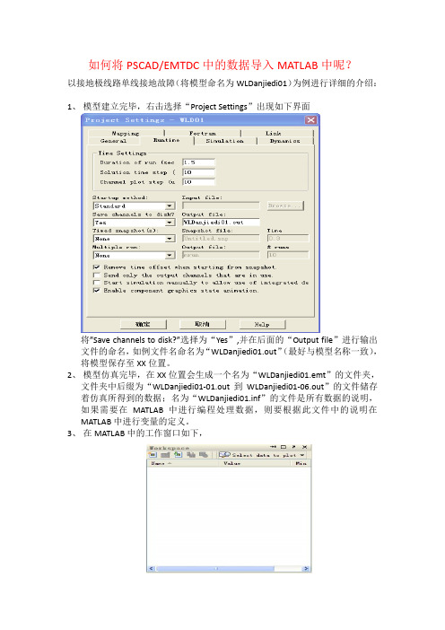
如何将PSCAD/EMTDC中的数据导入MATLAB中呢?
以接地极线路单线接地故障(将模型命名为WLDanjiedi01)为例进行详细的介绍:1、模型建立完毕,右击选择“Project Settings”出现如下界面
将”Save channels to disk?”选择为“Yes”,并在后面的“Output file”进行输出文件的命名,如例文件名命名为“WLDanjiedi01.out”(最好与模型名称一致),将模型保存至XX位置。
2、模型仿真完毕,在XX位置会生成一个名为“WLDanjiedi01.emt”的文件夹,
文件夹中后缀为“WLDanjiedi01-01.out到WLDanjiedi01-06.out”的文件储存着仿真所得到的数据;名为“WLDanjiedi01.inf”的文件是所有数据的说明,如果需要在MATLAB中进行编程处理数据,则要根据此文件中的说明在MATLAB中进行变量的定义。
3、在MATLAB中的工作窗口如下,
单击“Import data”找到“WLDanjiedi01.emt”目录,界面如下
下拉文件类型(T)选择“All Files(*.*)”出现如下界面
选择“WLDanjiedi01-01.out到WLDanjiedi01-06.out”中所需要的即可,例如导入“WLDanjiedi01-01.out”,选中后点击打开,经过一定时间会出现如下界面
选择“Next”,接着选择“Finish”即可完成数据的导入,此时MATLAB中的工作窗口如下,出现了“WLDanjiedi01-01”文件夹。
选中“WLDanjiedi01-01”,界面变成如下,单击“Plot(WLDanjiedi01-01)”会生成此文件夹所包含数据的波形图。
双击“WLDanjiedi01-01”出现如下界面
随便选中某一列然后点击上方的“Plot(WLDanjiedi01-01)”即可生成此列所表示的数据波形图。