克鲁格曼国际经济学课后答案英语版
克鲁格曼《国际经济学》第八版课后答案(英文)-Ch18
Chapter 18The International Monetary System, 1870–1973Chapter OrganizationMacroeconomic Policy Goals in an Open EconomyInternal Balance: Full Employment and Price-Level StabilityExternal Balance: The Optimal Level of the Current Account International Macroeconomic Policy under the Gold Standard, 1870–1914 Origins of the Gold StandardExternal Balance under the Gold StandardThe Price-Specie-Flow MechanismThe Gold Standard “Rules of the Game”: Myth and RealityBox: Hume v. the MercantilistsInternal Balance under the Gold StandardCase Study: The Political Economy of Exchange Rate Regimes:Conflict over America’s Monetary Standard During the 1890s The Interwar Years, 1918–1939The Fleeting Return to GoldInternational Economic DisintegrationCase Study: The International Gold Standard and the Great DepressionThe Bretton Woods System and the International Monetary Fund Goals and Structure of the IMFConvertibility and the Expansion of Private Capital FlowsSpeculative Capital Flows and CrisesAnalyzing Policy Options under the Bretton Woods System Maintaining Internal BalanceMaintaining External BalanceExpenditure-Changing and Expenditure-Switching PoliciesThe External-Balance Problem of the United StatesCase Study: The Decline and Fall of the Bretton Woods System Worldwide Inflation and the Transition to Floating Rates SummaryChapter OverviewThis is the first of five international monetary policy chapters. These chapters complement the preceding theory chapters in several ways. They provide the historical and institutional background students require to place their theoretical knowledge in a useful context. The chapters also allow students, through study of historical and current events, to sharpen their grasp of the theoretical models and to develop the intuition those models can provide. (Application of the theory to events of current interest will hopefully motivate students to return to earlier chapters and master points that may have been missed on the first pass.)Chapter 18 chronicles the evolution of the international monetary system from the gold standard of1870–1914, through the interwar years, and up to and including the post-World War II Bretton Woods regime that ended in March 1973. The central focus of the chapter is the manner in which each system addressed, or failed to address, the requirements of internal and external balance for its participants.A country is in internal balance when its resources are fully employed and there is price level stability. External balance implies an optimal time path of the current account subject to its being balanced over the long run. Other factors have been important in the definition of external balance at various times, and these are discussed in the text. The basic definition of external balance as an appropriate current-account level, however, seems to capture a goal that most policy-makers share regardless of the particular circumstances.The price-specie-flow mechanism described by David Hume shows how the gold standard could ensure convergence to external balance. You may want to present the following model of the price-specie-flow mechanism. This model is based upon three equations: 1. The balance sheet of the central bank. At the most simple level, this is justgold holdings equals the money supply: G M.2. The quantity theory. With velocity and output assumed constant and bothnormalized to 1, this yields the simple equation M P.3. A balance of payments equation where the current account is a function of thereal exchange rate and there are no private capital flows: CA f(E P*/P)These equations can be combined in a figure like the one below. The 45 line represents the quantity theory, and the vertical line is the price level where the real exchange rate results in a balanced current account. The economy moves along the 45 line back towards the equilibrium Point 0 whenever it is out of equilibrium. For example, the loss of four-fifths of a country’s gold would put that country at Point a with lower prices and a lower money supply. The resulting real exchange rate depreciation causes a current account surplus which restores money balances as the country proceeds up the 45 line froma to 0.FigureThe automatic adjustment process described by the price-specie-flow mechanism is expedited by following “rules of the game” under which governments contract the domestic source components oftheir monetary bases when gold reserves are falling (corresponding to a current-account deficit) and expand when gold reserves are rising (the surplus case).In practice, there was little incentive for countries with expanding gold reserves to follow the “rules of the game.” This increased the contractionary burden shouldered by countries with persistent current account deficits. The gold standard also subjugated internal balance to the demands of external balance. Research suggests price-level stability and high employment were attained less consistently under the gold standard than in the post-1945 period.The interwar years were marked by severe economic instability. The monetization of war debt and of reparation payments led to episodes of hyperinflation in Europe. Anill-fated attempt to return to thepre-war gold parity for the pound led to stagnation in Britain. Competitive devaluations and protectionism were pursued in a futile effort to stimulate domestic economic growth during the Great Depression.These beggar-thy-neighbor policies provoked foreign retaliation and led to the disintegration of the world economy. As one of the case studies shows, strict adherence to the Gold Standard appears to have hurt many countries during the Great Depression.Determined to avoid repeating the mistakes of the interwar years, Allied economic policy-makers metat Bretton Woods in 1944 to forge a new international monetary system for the postwar world. The exchange-rate regime that emerged from this conference had at its center the . dollar. All other currencies had fixed exchange rates against the dollar, which itself had a fixed value in terms of gold.An International Monetary Fund was set up to oversee the system and facilitate its functioning by lending to countries with temporary balance of payments problems.A formal discussion of internal and external balance introduces the concepts of expenditure-switching and expenditure-changing policies. The Bretton Woods system, with its emphasis on infrequent adjustmentof fixed parities, restricted the use of expenditure-switching policies. Increases in U.S. monetary growth to finance fiscal expenditures after the mid-1960s led to a loss of confidence in the dollar and the termination of the dollar’s convertibility into gold. The analysis presented in the text demonstrateshow the Bretton Woods system forced countries to “import” inflation from the United States and shows that the breakdown of the system occurred when countries were no longer willing to accept this burden.Answers to Textbook Problems1. a. Since it takes considerable investment to develop uranium mines, you wouldwant a larger current account deficit to allow your country to finance some of the investment with foreign savings.b. A permanent increase in the world price of copper would cause a short-termcurrent account deficit if the price rise leads you to invest more in coppermining. If there are no investment effects, you would not change yourexternal balance target because it would be optimal simply to spend youradditional income.c. A temporary increase in the world price of copper would cause a currentaccount surplus. You would want to smooth out your country’s consumption bysaving some of its temporarily higher income.d. A temporary rise in the world price of oil would cause a current accountdeficit if you were an importer of oil, but a surplus if you were an exporter of oil.2. Because the marginal propensity to consume out of income is less than 1, atransfer of income from B to A increases savings in A and decreases savings in B.Therefore, A has a current account surplus and B has a corresponding deficit.This corresponds to a balance of payments disequilibrium in Hume’s world, which must be financed by gold flows from B to A. These gold flows increase A’s money supply and decrease B’s money supply, pushing up prices in A and depressingprices in B. These price changes cease once balance of payments equilibrium has been restored.3. Changes in parities reflected both initial misalignments and balance of paymentscrises. Attempts to return to the parities of the prewar period after the war ignored the changes in underlying economic fundamentals that the war caused. This made some exchange rates less than fully credible and encouraged balance ofpayments crises. Central bank commitments to the gold parities were also less than credible after the wartime suspension of the gold standard, and as a result of the increasing concern of governments with internal economic conditions.4. A monetary contraction, under the gold standard, will lead to an increase in thegold holdings of the contracting country’s central bank if other countries do not pursue a similar policy. All countries cannot succeed in doing thissimultaneously since the total stock of gold reserves is fixed in the short run.Under a reserve currency system, however, a monetary contraction causes anincipient rise in the domestic interest rate, which attracts foreign capital. The central bank must accommodate the inflow of foreign capital to preserve theexchange rate parity. There is thus an increase in the central bank’s holdings of foreign reserves equal to the fall in its holdings of domestic assets. There is no obstacle to a simultaneous increase in reserves by all central banksbecause central banks acquire more claims on the reserve currency country while their citizens end up with correspondingly greater liabilities.5. The increase in domestic prices makes home exports less attractive and causes acurrent account deficit. This diminishes the money supply and causescontractionary pressures in the economywhich serve to mitigate and ultimately reverse wage demands and price increases.6. A “demand determined” increase in dollar reserve holdings would not affect theworld supply of money as central banks merely attempt to trade their holdings of domestic assets for dollar rese rves. A “supply determined” increase in reserve holdings, however, would result from expansionary monetary policy in the United States (the reserve center). At least at the end of the Bretton Woods era the increase in world dollar reserves arose in part because of an expansionarymonetary policyin the United States rather than a desire by other central banks to increasetheir holdings of dollar assets. Only the “supply determined” increase indollar reserves is relevant for analyzing the relationship between world holdings of dollar reserves by central banks and inflation.7. An increase in the world interest rate leads to a fall in a central bank’sholdings of foreign reserves as domestic residents trade in their cash forforeign bonds. This leads to a d ecline in the home country’s money supply. The central bank of a “small” country cannot offset these effects sinceit cannot alter the world interest rate. An attempt to sterilize the reserve loss through open market purchases would fail unless bonds are imperfect substitutes.8. Capital account restrictions insulate the domestic interest rate from the worldinterest rate. Monetary policy, as well as fiscal policy, can be used to achieve internal balance. Because there are no offsetting capital flows, monetary policy, as well as fiscal policy, can be used to achieve internal balance. The costs of capital controls include the inefficiency which is introduced when the domestic interest rate differs from the world rate and the high costs of enforcing the controls.9. Yes, it does seem that the external balance problem of a deficit country is moresevere. While the macroeconomic imbalance may be equally problematic in the long run regardless of whether it is a deficit or surplus, large external deficits involve the risk that the market will fix the problem quickly by ceasing to fund the external deficit. In this case, there may have to be rapid adjustment that could be disruptive. Surplus countries are rarely forced into rapid adjustments, making the problems less risky.10. An inflow attack is different from capital flight, but many parallels exist. Inan “outflow” attack, speculators sell the home currency and drain the central bank of its foreign assets. The central bank could always defend if it so chooses (they can raise interest rates to improbably high levels), but if it is unwilling to cripple the economy with tight monetary policy, it must relent. An “inflow”attack is similar in that the central bank can always maintain the peg, it is just that the consequences of doing so may be more unpalatable than breaking the peg. If money flows in, the central bank must buy foreign assets to keep thecurrency from appreciating. If the central bank cannot sterilize all the inflows (eventually they may run out of domestic assets to sell to sterilize thetransactions where they are buying foreign assets), it will have to either let the currency appreciate or let the money supply rise. If it is unwilling to allow and increase in inflation due to a rising money supply, breaking the peg may be preferable.11. a. We know that China has a very large current account surplus, placing them highabove the XX line. They also have moderate inflationary pressures (describedas “gathering” in the question, implying they are not yet very strong). This suggests that China is above the II line, but not too far above it. It wouldbe placed in Zone 1 (see below).b. China needs to appreciate the exchange rate to move down on the graph towardsbalance. (Shown on the graph with the dashed line down)c. China would need to expand government spending to move to the right and hitthe overall balance point. Such a policy would help cushion the negative aggregate demand pressurethat the appreciation might generate.。
克鲁格曼《国际经济学》第八版课后答案(英文)-Ch08

Chapter 8The Instruments of Trade PolicyChapter OrganizationBasic Tariff AnalysisSupply, Demand, and Trade in a Single IndustryEffects of a TariffMeasuring the Amount of ProtectionCosts and Benefits of a TariffConsumer and Producer SurplusMeasuring the Costs and BenefitsOther Instruments of Trade PolicyExport Subsidies: TheoryCase Study: Europe’s Common Agricultural PolicyImport Quotas: TheoryCase Study: An Import Quota in Practice: U.S. SugarVoluntary Export RestraintsCase Study: A Voluntary Export Restraint in Practice: Japanese Autos Local Content RequirementsBox: American Buses, Made in HungaryOther Trade Policy InstrumentsThe Effects of Trade Policy: A SummarySummaryAppendix I: Tariff Analysis in General EquilibriumA Tariff in a Small CountryA Tariff in a Large CountryAppendix II: Tariffs and Import Quotas in the Presence of Monopoly The Model with Free TradeThe Model with a TariffThe Model with an Import QuotaComparing a Tariff with a QuotaChapter 8 The Instruments of Trade Policy 33Chapter OverviewThis chapter and the next three focus on international trade policy. Students will have heard various arguments for and against restrictive trade practices in the media. Some of these arguments are sound and some are clearly not grounded in fact. This chapter provides a framework for analyzing the economic effects of trade policies by describing the tools of trade policy and analyzing their effects on consumers and producers in domestic and foreign countries. Case studies discuss actual episodes of restrictive trade practices. An instructor might try to underscore the relevance of these issues by having students scan newspapers and magazines for other timely examples of protectionism at work.The analysis presented here takes a partial equilibrium view, focusing on demand and supply in one market, rather than the general equilibrium approach followed in previous chapters. Import demand and export supply curves are derived from domestic and foreign demand and supply curves. There are a number of trade policy instruments analyzed in this chapter using these tools. Some of the important instruments of trade policy include specific tariffs, defined as taxes levied as a fixed charge for each unit of a good imported; ad valorem tariffs, levied as a fraction of the value of the imported good; export subsidies, which are payments given to a firm or industry that ships a good abroad; import quotas, which are direct restrictions on the quantity of some good that may be imported; voluntary export restraints, which are quotas on trading that are imposed by the exporting country instead of the importing country; and local content requirements, which are regulations that require that some specified fraction of a good is produced domestically.The import supply and export demand analysis demonstrates that the imposition of a tariff drives a wedge between prices in domestic and foreign markets, and increases prices in the country imposing the tariff and lowers the price in the other country by less than the amount of the tariff. This contrasts with most textbook presentations which make the small country assumption that the domestic internal price equals the world price times one plus the tariff rate. The actual protection provided by a tariff willnot equal the tariff rate if imported intermediate goods are used in the production of the protected good. The proper measurement, the effective rate of protection, is described in the text and calculated for a sample problem.The analysis of the costs and benefits of trade restrictions require tools of welfare analysis. The text explains the essential tools of consumer and producer surplus. Consumer surplus on each unit sold is defined as the difference between the actual price and the amount that consumers would have been willing to pay for the product. Geometrically, consumer surplus is equal to the area under the demand curve and above the price of the good. Producer surplus is the difference between the minimum amount for which a producer is willing to sell his product and the price which he actually receives. Geometrically, producer surplus is equal to the area above the supply curve and below the price line. These tools are fundamental to the student’s understanding of the implications of trade polici es and should be developed carefully. The costs of a tariff include distortionary efficiency losses in both consumption and production. A tariff provides gains from terms of trade improvement when and if it lowers the foreign export price. Summing the areas in a diagram of internal demand and supply provides a method for analyzing the net loss or gain from a tariff.Other instruments of trade policy can be analyzed with this method. An export subsidy operates in exactly the reverse fashion of an import tariff. An import quota has similar effects as an import tariff upon prices and quantities, but revenues, in the form of quota rents, accrue to foreign producers of the protected good. Voluntary export restraints are a form of quotas in which import licenses are held by foreign governments. Local content requirements raise the price of imports and domestic goods and do not result in either government revenue or quota rents.34 Krugman/Obstfeld •International Economics: Theory and Policy, Eighth EditionThroughout the chapter the analysis of different trade restrictions are illustrated by drawing upon specific episodes. Europe’s common agricultural policy provides and example of export subsidies in action. The case study corresponding to quotas describes trade restrictions on U.S. sugar imports. Voluntary export restraints are discussed in the context of Japanese auto sales to the United States. The oil import quota in the United States in the 1960’s provides an example of a local content scheme.There are two appendices to this chapter. Appendix I uses a general equilibrium framework to analyze the impact of a tariff, departing from the partial equilibrium approach taken in the chapter. When a small country imposes a tariff, it shifts production away from its exported good and toward the imported good. Consumption shifts toward the domestically produced goods. Both the volume of trade and welfare of the country decline. A large country imposing a tariff can improve its terms of trade by an amount potentially large enough to offset the production and consumption distortions. For a large country, a tariff may be welfare improving.Appendix II discusses tariffs and import quotas in the presence of a domestic monopoly. Free trade eliminates the monopoly power of a domestic producer and the monopolist mimics the actions of a firm in a perfectly competitive market, setting output such that marginal cost equals world price. A tariff raises domestic price. The monopolist, still facing a perfectly elastic demand curve, sets output such that marginal cost equals internal price. A monopolist faces a downward sloping demand curve under a quota.A quota is not equivalent to a tariff in this case. Domestic production is lower and internal price higher when a particular level of imports is obtained through the imposition of a quota rather than a tariff.Answers to Textbook Problems1. The import demand equation, MD, is found by subtracting the home supply equation from the homedemand equation. This results in MD= 80 - 40 ⨯P. Without trade, domestic prices and quantities adjust such that import demand is zero. Thus, the price in the absence of trade is 2.2. a. Foreign’s export supply curve, XS, is XS=-40 + 40⨯P. In the absence of trade, the price is 1.b. When trade occurs, export supply is equal to import demand, XS=MD. Thus, using theequations from Problems 1 and 2a, P= 1.50, and the volume of trade is 20.3. a. The new MD curve is 80 - 40 ⨯ (P+ t) where t is the specific tariff rate, equal to 0.5. (Note: Insolving these problems, you should be careful about whether a specific tariff or ad valorem tariff is imposed. With an ad valorem tariff, the MD equation would be expressed as MD= 80 - 40 ⨯(1 + t)P.) The equation for the export supply curve by the foreign country is unchanged. Solving,we find that the world price is $1.25, and thus the internal price at home is $1.75. The volume of trade has been reduced to 10, and the total demand for wheat at home has fallen to 65 (from thefree trade level of 70). The total demand for wheat in Foreign has gone up from 50 to 55.b. andc. The welfare of the home country is best studied using the combined numerical andgraphical solutions presented below in Figure 8.1.Figure 8.1Chapter 8 The Instruments of Trade Policy 35where the areas in the figure are:a.55(1.75 - 1.50) -0.5(55 - 50)(1.75 - 1.50) = 13.125b. 0.5(55 - 50)(1.75 - 1.50) = 0.625c. (65 - 55)(1.75 - 1.50) = 2.50d. 0.5(70 - 65)(1.75 - 1.50) = 0.625e. (65 - 55)(1.50 - 1.25) = 2.50Consumer surplus change: -(a+ b+ c+ d) =-16.875. Producer surplus change: a= 13.125.Government revenue change: c+ e= 5. Efficiency losses b+ d are exceeded by terms of tradegain e. (Note: In the calculations for the a, b, and d areas, a figure of 0.5 shows up. This isbecause we are measuring the area of a triangle, which is one-half of the area of the rectangledefined by the product of the horizontal and vertical sides.)4. Using the same solution methodology as in Problem 3, when the home country is very small relativeto the foreign country, its effects on the terms of trade are expected to be much less. The smallcountry is much more likely to be hurt by its imposition of a tariff. Indeed, this intuition is shown in this problem. The free trade equilibrium is now at the price $1.09 and the trade volume is now$36.40.With the imposition of a tariff of 0.5 by Home, the new world price is $1.045, the internal home price is $1.545, home demand is 69.10 units, home supply is 50.90, and the volume of trade is 18.20.When Home is relatively small, the effect of a tariff on world price is smaller than when Home is relatively large. When Foreign and Home were closer in size, a tariff of 0.5 by home lowered world price by 25 percent, whereas in this case the same tariff lowers world price by about 5 percent. The internal Home price is now closer to the free trade price plus t than when Home was relatively large.In this case, the government revenues from the tariff equal 9.10, the consumer surplus loss is 33.51, and the producer surplus gain is 21.089. The distortionary losses associated with the tariff (areas b+ d) sum to 4.14 and the terms of trade gain (e) is 0.819. Clearly, in this small country example, the distortionary losses from the tariff swamp the terms of trade gains. The general lesson is the smaller the economy, the larger the losses from a tariff since the terms of trade gains are smaller.5. ERP = (200 ⨯ 1.50 - 200)/100 = 100%6. The effective rate of protection takes into consideration the costs of imported intermediate goods.Here, 55% of the cost can be imported, suggesting with no distortion, home value added would be 45%. A 15% increase in the price of ethanol, though, means home value added could be as high as 60%. Effective rate of protection = (V t-V w)/V w, where V t is the value added in the presence of trade policies, and V w is the value added without trade distortions. In this case, we have (60 - 45)/45 = 33% effective rate of protection.7. We first use the foreign export supply and domestic import demand curves to determine the newworld price. The foreign supply of exports curve, with a foreign subsidy of 50 percent per unit,becomes XS=-40 + 40(1 + 0.5) ⨯P. The equilibrium world price is 1.2 and the internal foreign price is 1.8. The volume of trade is 32. The foreign demand and supply curves are used to determine the costs and benefits of the subsidy. Construct a diagram similar to that in the text and calculate the area of the various polygons. The government must provide (1.8 - 1.2)⨯ 32 = 19.2 units of output to support the subsidy. Foreign producers surplus rises due to the subsidy by the amount of 15.3 units of output. Foreign consumers surplus falls due to the higher price by 7.5 units of the good. Thus, the net loss to Foreign due to the subsidy is 7.5 + 19.2 - 15.3 = 11.4 units of output. Home consumers and producers face an internal price of 1.2 as a result of the subsidy. Home consumers surplus rises by 70 ⨯ 0.3 + 0.5 (6⨯ 0.3) = 21.9, while Home producers surplus falls by 44 ⨯ 0.3 + 0.5(6 ⨯ 0.3) =14.1, for a net gain of 7.8 units of output.36 Krugman/Obstfeld •International Economics: Theory and Policy, Eighth Edition8. a. False, unemployment has more to do with labor market issues and the business cycle than withtariff policy.b. False, the opposite is true because tariffs by large countries can actually reduce world priceswhich helps offset their effects on consumers.c. This kind of policy might reduce automobile production and Mexico, but also would increase theprice of automobiles in the United States, and would result in the same welfare loss associatedwith any quota.9. At a price of $10 per bag of peanuts, Acirema imports 200 bags of peanuts. A quota limiting theimport of peanuts to 50 bags has the following effects:a. The price of peanuts rises to $20 per bag.b. The quota rents are ($20 - $10) ⨯ 50 = $500.c. The consumption distortion loss is 0.5 ⨯ 100 bags ⨯ $10 per bag = $500.d. The production distortion loss is 0.5 ⨯ 50 bags ⨯ $10 per bag = $250.10. The reason is largely that the benefits of these policies accrue to a small group of people and thecosts are spread out over many people. Thus, those that benefit care far more deeply about these policies. These typical political economy problems associated with trade policy are probably even more troublesome in agriculture, where there are long standing cultural reasons for farmers andfarming communities to want to hold onto their way of life, making the interests even moreentrenched than they would normally be.11. It would improve the income distribution within the economy since wages in manufacturing wouldincrease, and real incomes for others in the economy would decrease due to higher prices formanufactured goods. This is true only under the assumption that manufacturing wages are lower than all others in the economy. If they were higher than others in the economy, the tariff policies would worsen the income distribution.。
克鲁格曼《国际经济学》第八版课后答案(英文)-Ch02.doc
Chapter 2World Trade: An Overview⏹Chapter OrganizationWho Trades with Whom?Size Matters: the Gravity ModelThe Logic of the Gravity ModelUsing the Gravity Model: Looking for AnomaliesImpediments to Trade: Distance, Barriers, and BordersThe Changing Pattern of World TradeHas the World Gotten SmallerWhat Do We Trade?Service OutsourcingDo Old Rules Still Apply?Summary⏹Key ThemesBefore entering into a series of theoretical models that explain why countries trade across borders and the benefits of this trade (Chapters 3–11), Chapter 2 considers the pattern of world trade which we observe today. The core idea of the chapter is the empirical model known as the gravity model. The gravity model is based on the observations that: (1) countries tend to trade with other nearby economies and (2) countries’ trade is proportional to their size. The model is called the gravity model as it is similar in form to the physics equation that describes the pull of one body on another as proportional to their size and distance.The basic form of the gravity equation is T ij=A⨯Y i⨯Y j/D ij. The logic supporting this equation is that large countries have large incomes to spend on imports and produce a large quantity of goods to sell as exports. This means that the larger either trade partner, the larger the volume of trade between them. At the same time, the distance between two trade partners can substitute for the transport costs that they face as well as proxy for more intangible aspects of a trading relationship such as the ease of contact for firms. This model can be used to estimate the predicted trade between two countries and look for anomalies in trade patterns. The text shows an example where the gravity model can be used to demonstrate the importance of national borders in determining trade flows. According to many estimates, the border between the U.S. and Canada has the impact on trade equivalent to roughly 2000 miles of distance. Other factors, such as tariffs, trade agreements, and common language can all affect trade and can be incorporated into the gravity model.The chapter also considers the way trade has evolved over time. While people often feel that the modern era has seen unprecedented globalization, in fact, there is precedent. From the end of the 19th century to World War I, the economies of different countries were quite connected. Trade as a share of GDP was higher in 1910 than 1960, and only recently have trade levels surpassed the pre World War trade. The nature of trade has change though. The majority of trade is in manufactured goods with agriculture and mineral products (and oil) making up less than 20% of world trade. Even developing countries now export primarily manufactures. In contrast, a century ago, more trade was in primary products as nations tended to trade for things that literally could not be grown or found at home. Today, the reasons for trade are more varied and the products we trade are ever changing (for example, the rise in trade of things like call centers). Th e chapter concludes by focusing on one particular expansion of what is “tradable”—the increase in services trade. Modern information technology has greatly expanded what can be traded as the person staffing a call center, doing your accounting, or reading your X-ray can literally be half-way around the world. While still relatively rare, the potential for a large increase in service outsourcing is an important part of how trade will evolve in the coming decades. The next few chapters will explain the theory of why nations trade.Answers to Textbook Problems1. We saw that not only is GDP important in explaining how much two countries trade, but also,distance is crucial. Given its remoteness, Australia faces relatively high costs of transporting imports and exports, thereby reducing the attractiveness of trade. Since Canada has a border with a largeeconomy (the U.S.) and Australia is not near any other major economy, it makes sense that Canada would be more open and Australia more self-reliant.2. Mexico is quite close to the U.S., but it is far from the European Union (EU). So it makes sense thatit trades largely with the U.S. Brazil is far from both, so its trade is split between the two. Mexico trades more than Brazil in part because it is so close to a major economy (the U.S.) and in partbecause it is a member of a free trade agreement with a large economy (NAFTA). Brazil is farther away from any large economy and is in a free trade agreement with relatively small countries.3. No, if every country’s GDP were to double, world trade would not quadruple. One way to see thisusing the example from Table 2-2 would simply be to quadruple all the trade flows in 2-2 and also double the GDP in 2-1. We would see that the first line of Table 2-2 would be—, 6.4, 1.6, 1.6. If that were true, Country A would have exported $8 trillion which is equal to its entire GDP. Likewise, it would have imported $8 trillion, meaning it had zero spending on its own goods (highly unlikely). If instead we filled in Table 2-2 as before, by multiplying the appropriate shares of the world economy times a country’s GDP, we would see the first line of Table 2-2 reads—, 3.2, 0.8, 0.8. In this case, 60% of Country A’s GDP is exported, the same as before. The logic is that while the world G DP has doubled, increasing the likelihood of international trade, the local economy has doubled, increasing the likelihood of domestic trade. The gravity equation still holds. If you fill in the entire table, you will see that where before the equation was 0.1 ⨯ GDP i⨯ GDP j, it now is 0.05 ⨯ GDP i⨯ GDP j. The coefficient on each GDP is still one, but the overall constant has changed.4. As the share of world GDP which belongs to East Asian economies grows, then in every traderelationship which involves an East Asian economy, the size of the East Asian economy has grown.This makes the trade relationships with East Asian countries larger over time. The logic is similar for why the countries trade more with one another. Previously, they were quite small economies, meaning that their markets were too small to import a substantial amount. As they became morewealthy and the consumption demands of their populace rose, they were each able to importmore. Thus, while they previously had focused their exports to other rich nations, over time, they became part of the rich nation club and thus were targets for one another’s exports. Again, using the gravity model, when South Korea and Taiwan were both small, the product of their GDPs was quite small, meaning despite their proximity, there was little trade between them. Now that they have both grown considerably, their GDPs predict a considerable amount of trade.5. As the chapter discusses, a century ago, much of world trade was in commodities that in many wayswere climate or geography determined. Thus, the UK imported goods that it could not make itself.This meant importing things like cotton or rubber from countries in the Western Hemisphere or Asia.As the UK’s climate and natural resource endowments were fairly similar to those in the rest of Europe, it had less of a need to import from other European countries. In the aftermath of the IndustrialRevolution, where manufacturing trade accelerated and has continued to expand with improvements in transportation and communications, it is not surprising that the UK would turn more to the nearby and large economies in Europe for much of its trade. This is a direct prediction of the gravity model.。
克鲁格曼《国际经济学》第八版课后答案(英文)-Ch05
Chapter 5The Standard Trade ModelChapter OrganizationA Standard Model of a Trading EconomyProduction Possibilities and Relative SupplyRelative Prices and DemandThe Welfare Effect of Changes in the Terms of TradeDetermining Relative PricesEconomic Growth: A Shift of the RS CurveGrowth and the Production Possibility FrontierRelative Supply and the Terms of TradeInternational Effects of GrowthCase Study: Has the Growth of Newly Industrializing Countries Hurt Advanced Nations? International Transfers of Income: Shifting the RD CurveThe Transfer ProblemEffects of a Transfer on the Terms of TradePresumptions about the Terms of Trade Effects of TransfersCase Study: The Transfer Problem and the Asian CrisisTariffs and Export Subsidies: Simultaneous Shifts in RS and RDRelative Demand and Supply Effects of a TariffEffects of an Export SubsidyImplications of Terms of Trade Effects: Who Gains and Who Loses?SummaryAppendix: Representing International Equilibrium with Offer CurvesDeriving a Country’s Offer CurveInternational EquilibriumChapter 5 The Standard Trade Model 17Chapter OverviewPrevious chapters have highlighted specific sources of comparative advantage which give rise to international trade. This chapter presents a general model which admits previous models as special cases. This “standard trade model” is the workhorse of international trade theory and can be used to address a wide range of issues. Some of these issues, such as the welfare and distributional effects of economic growth, transfers between nations, and tariffs and subsidies on traded goods are considered in this chapter. The standard trade model is based upon four relationships. First, an economy will produce at the point where the production possibilities curve is tangent to the relative price line (called the isovalue line). Second, indifference curves describe the tastes of an economy, and the consumption point for that economy is found at the tangency of the budget line and the highest indifference curve. These two relationships yield the familiar general equilibrium trade diagram for a small economy (one which takes as given the terms of trade), where the consumption point and production point are the tangencies of the isovalue line with the highest indifference curve and the production possibilities frontier, respectively.You may want to work with this standard diagram to demonstrate a number of basic points. First, an autarkic economy must produce what it consumes, which determines the equilibrium price ratio; and second, opening an economy to trade shifts the price ratio line and unambiguously increases welfare. Third, an improvement in the terms of trade increases welfare in the economy. Fourth, it is straightforward to move from a small country analysis to a two country analysis by introducing a structure of world relative demand and supply curves which determine relative prices.These relationships can be used in conjunction with the Rybczynski and the Stolper-Samuelson Theorems from the previous chapter to address a range of issues. For example, you can consider whether the dramatic economic growth of countries like Japan and Korea has helped or hurt the United States as a whole, and also identify the classes of individuals within the United States who have been hurt by the particular growth biases of these countries. In teaching these points, it might be interesting and useful to relate them to current events. For example, you can lead a class discussion of the implications for the United States of the provision of forms of technical and economic assistance to the emerging economies around the world or the ways in which a world recession can lead to a fall in demand for U.S. export goods.The example provided in the text considers the popular arguments in the media that growth in Japan or Korea hurts the United States. The analysis presented in this chapter demonstrates that the bias of growth is important in determining welfare effects rather than the country in which growth occurs. The existence of biased growth, and the possibility of immiserizing growth is discussed. The Relative Supply (RS) and Relative Demand (RD) curves illustrate the effect of biased growth on the terms of trade. The new terms of trade line can be used with the general equilibrium analysis to find the welfare effects of growth. A general principle which emerges is that a country which experiences export-biased growth will have a deterioration in its terms of trade, while a country which experiences import-biased growth has an improvement in its terms of trade. A case study points out that growth in the rest of the world has made other countries more like the United States. This import-biased growth has worsened the terms of trade for the United States. The second issue addressed in the context of the standard trade model is the effect of international transfers. The salient point here is the direction, if any, in which the relative demand curve shifts in response to the redistribution of income from a transfer. A transfer worsens the donor’s ter ms of trade if it has a higher marginal propensity to consume its export good than the recipient. The presence of non-traded goods tends to reinforce the deterioration of terms of trade for the donor country. The case study attendant to this issue involves the deterioration of many Asian countries’ terms of trade due to the large capital withdrawals at the end of the 1990s.18 Krugman/Obstfeld •International Economics: Theory and Policy, Eighth EditionThe third area to which the standard trade model is applied are the effects of tariffs and export subsidies on welfare and terms of trade. The analysis proceeds by recognizing that tariffs or subsidies shift both the relative supply and relative demand curves. A tariff on imports improves the terms of trade, expressed in external prices, while a subsidy on exports worsens terms of trade. The size of the effect depends upon the size of the country in the world. Tariffs and subsidies also impose distortionary costs upon the economy. Thus, if a country is large enough, there may be an optimum, non-zero tariff. Export subsidies, however, only impose costs upon an economy. Intranationally, tariffs aid import-competing sectors and hurt export sectors while subsidies have the opposite effect. An appendix presents offer curve diagrams and explains this mode of analysis.Answers to Textbook Problems1.Note how welfare in both countries increases as the two countries move from productionpatterns governed by domestic prices (dashed line) to production patterns governed by worldprices (straight line).2.3. An increase in the terms of trade increases welfare when the PPF is right-angled. The production pointis the corner of the PPF. The consumption point is the tangency of the relative price line and the highest indifference curve. An improvement in the terms of trade rotates the relative price line about its intercept with the PPF rectangle (since there is no substitution of immobile factors, the production point stays fixed). The economy can then reach a higher indifference curve. Intuitively, although there is no supply response, the economy receives more for the exports it supplies and pays less for the imports it purchases.Chapter 5 The Standard Trade Model 19 4. The difference from the standard diagram is that the indifference curves are right angles rather thansmooth curves. Here, a terms of trade increase enables an economy to move to a higher indifference curve. The income expansion path for this economy is a ray from the origin. A terms of tradeimprovement moves the consumption point further out along the ray.5. The terms of trade of Japan, a manufactures (M) exporter and a raw materials (R) importer, is the worldrelative price of manufactures in terms of raw materials (p M/p R). The terms of trade change can be determined by the shifts in the world relative supply and demand (manufactures relative to raw materials) curves. Note that in the following answers, world relative supply (RS) and relative demand (RD) are always M relative to R. We consider all countries to be large, such that changes affect the world relative price.a. Oil supply disruption from the Middle East decreases the supply of raw materials, which increasesthe world relative supply. The world relative supply curve shifts out, decreasing the world relative price of manufactured goods and deteriorating Japan’s terms of t rade.b. Korea’s increased automobile production increases the supply of manufactures, which increasesthe world RS. The world relative supply curve shifts out, decreasing the world relative price ofmanufactured goods and deteriorating Japan’s terms of tr ade.c. U.S. development of a substitute for fossil fuel decreases the demand for raw materials. Thisincreases world RD, and the world relative demand curve shifts out, increasing the world relative price of manufactured goods and improving Japan’s terms of trade. This occurs even if no fusion reactors are installed in Japan since world demand for raw materials falls.d. A harvest failure in Russia decreases the supply of raw materials, which increases the world RS.The world relative supply curve shifts o ut. Also, Russia’s demand for manufactures decreases,which reduces world demand so that the world relative demand curve shifts in. These forcesdecrease the world relative price of manufactured goods and deteriorate Japan’s terms of trade.e. A reduction in Japan’s tariff on raw materials will raise its internal relative price of manufactures.This price change will increase Japan’s RS and decrease Japan’s RD, which increases the worldRS and decreases the world RD (i.e., world RS shifts out and world RD shifts in). The worldrelative price of manufactures declines and Japan’s terms of trade deteriorate.6. The declining price of services relative to manufactured goods shifts the isovalue line clockwise sothat relatively fewer services and more manufactured goods are produced in the United States, thus reducing U.S. welfare.20 Krugman/Obstfeld •International Economics: Theory and Policy, Eighth Edition7. These results acknowledge the biased growth which occurs when there is an increase in one factor ofproduction. An increase in the capital stock of either country favors production of Good X, while an increase in the labor supply favors production of Good Y. Also, recognize the Heckscher-Ohlin result that an economy will export that good which uses intensively the factor which that economy has in relative abundance. Country A exports Good X to Country B and imports Good Y from Country B.The possibility of immiserizing growth makes the welfare effects of a terms of trade improvement due to export-biased growth ambiguous. Import-biased growth unambiguously improves welfare for the growing country.a. A’s terms of trade worsen, A’s welfare may increase or, less likely, decrease, and B’s welfareincreases.b. A’s terms of trade improve, A’s welfare increases and B’s welfare decreases.c. B’s terms of trade improve, B’s welfare increases and A’s welfare decreases.d. B’s terms of trade worsen, B’s welfare may increase or, less likely, decrease, and A’s welfareincreases.8. Immiserizing growth occurs when the welfare deteriorating effects of a worsening in an economy’sterms of trade swamp the welfare improving effects of growth. For this to occur, an economy must undergo very biased growth, and the economy must be a large enough actor in the world economy such that its actions spill over to adversely alter the terms of trade to a large degree. This combination of events is unlikely to occur in practice.9. India opening should be good for the U.S. if it reduces the relative price of goods that China sends tothe U.S. and hence increases the relative price of goods that the U.S. exports. Obviously, any sector in the U.S. hurt by trade with China would be hurt again by India, but on net, the U.S. wins. Note that here we are making different assumptions about what India produces and what is tradable than we are in Question #6. Here we are assuming India exports products the U.S. currently imports and China currently exports. China will lose by having the relative price of its export good driven down by the increased production in India.10. Aid which must be spent on exports increases the demand for those export goods and raises their pricerelative to other goods. There will be a terms of trade deterioration for the recipient country. This can be viewed as a polar case of the effect of a transfer on the terms of trade. Here, the marginal propensity to consume the export good by the recipient country is 1. The donor benefits from a terms of trade improvement. As with immiserizing growth, it is theoretically possible that a transfer actuallyworsens the welfare of the recipient.11. When a country subsidizes its exports, the world relative supply and relative demand schedules shiftsuch that the terms of trade for the country worsen. A countervailing import tariff in a second country exacerbates this effect, moving the terms of trade even further against the first country. The firstcountry is worse off both because of the deterioration of the terms of trade and the distortionsintroduced by the new internal relative prices. The second country definitely gains from the firstcountry’s export su bsidy, and may gain further from its own tariff. If the second country retaliated with an export subsidy, then this would offset the initial improvement in the terms of trade; the“retaliatory” export subsidy definitely helps the first country and hurts th e second.。
克鲁格曼《国际经济学》(国际金融部分)课后习题答案(英文版)第一章
克鲁格曼《国际经济学》(国际金融部分)课后习题答案(英文版)第一章CHAPTER 1INTRODUCTIONChapter OrganizationWhat is International Economics About?The Gains from TradeThe Pattern of TradeProtectionismThe Balance of PaymentsExchange-Rate DeterminationInternational Policy CoordinationThe International Capital MarketInternational Economics: Trade and MoneyCHAPTER OVERVIEWThe intent of this chapter is to provide both an overview of the subject matter of international economics and to provide a guide to the organization of the text. It is relatively easy for an instructor to motivate the study of international trade and finance. The front pages of newspapers, the covers of magazines, and the lead reports of television news broadcasts herald the interdependence of the U.S. economy with the rest of the world. This interdependence may also be recognized by students through their purchases of imports of all sorts of goods, their personal observations of the effects of dislocations due to international competition, and their experience through travel abroad.The study of the theory of international economics generates an understanding of many key events that shape our domesticand international environment. In recent history, these events include the causes and consequences of the large current account deficits of the United States; the dramatic appreciation of the dollar during the first half of the 1980s followed by its rapid depreciation in the second half of the 1980s; the Latin American debt crisis of the 1980s and the Mexico crisis in late 1994; and the increased pressures for industry protection against foreign competition broadly voiced in the late 1980s and more vocally espoused in the first half of the 1990s. Most recently, the financial crisis that began in East Asia in 1997 andspread to many countries around the globe and the Economic and Monetary Union in Europe have highlighted the way in which various national economies are linked and how important it is for us to understand these connections. At the same time, protests at global economic meetings have highlighted opposition to globalization. The text material will enable students to understand the economic context in which such events occur.Chapter 1 of the text presents data demonstrating the growth in trade and increasing importance of international economics. This chapter also highlights and briefly discusses seven themes which arise throughout the book. These themes include: 1) the gains from trade;2) the pattern of trade; 3) protectionism; 4), the balance of payments; 5) exchange rate determination; 6) international policy coordination; and 7) the international capital market. Students will recognize that many of the central policy debates occurring today come under the rubric of one of these themes. Indeed, it is often a fruitful heuristic to use current events to illustrate the force of the key themes and arguments which are presentedthroughout the text.。
国际经济学(克鲁格曼)教材答案
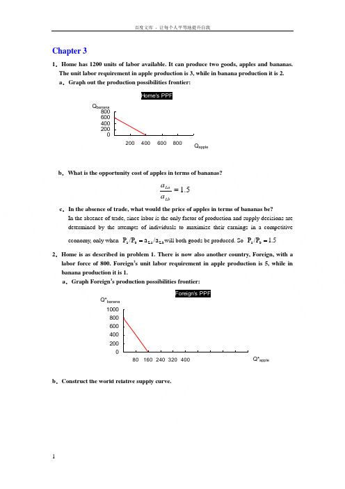
Chapter 31.Home has 1200 units of labor available. It can produce two goods, apples and bananas. The unit labor requirement in apple production is 3, while in banana production it is 2. a .Graph out the production possibilities frontier:b .What is the opportunity cost of apples in terms of bananas?5.1=LbLa a a c .In the absence of trade, what would the price of apples in terms of bananas be?In the absence of trade, since labor is the only factor of production and supply decisions aredetermined by the attempts of individuals to maximize their earnings in a competitive economy, only when Lb La b a /a a /P P =will both goods be produced. So 1.5 /P P b a =2.Home is as described in problem 1. There is now also another country, Foreign, with alabor force of 800. Foreign ’s unit labor requirement in apple production is 5, while in banana production it is 1.a .Graph Foreign ’s production possibilities frontier:b .Construct the world relative supply curve.Home's PPF 0200400600800200400600800Q apple Q banana Foreign's PPF0200400600800100080160240320400Q*apple Q*banana3.Now suppose world relative demand takes the following form: Demand for apples/demandfor bananas = price of bananas/price of apples.a .Graph the relative demand curve along with the relative supply curve:a b b a /P P /D D =∵When the market achieves its equilibrium, we have 1b a )(D D -**=++=ba b b a a P P Q Q Q Q ∴RD is a hyperbola xy 1=b .What is the equilibrium relative price of apples?The equilibrium relative price of apples is determined by the intersection of the RD and RScurves.RD: yx 1= RS: 5]5,5.1[5.1],5.0(5.0)5.0,0[=∈=⎪⎩⎪⎨⎧+∞∈=∈y y y x x x ∴25.0==y x∴2/=b P a P e ec .Describe the pattern of trade.∵b a b e a e b a P P P P P P ///>>**∴In this two-country world, Home will specialize in the apple production, export apples and import bananas. Foreign will specialize in the banana production, export bananas and import apples.d .Show that both Home and Foreign gain from trade.International trade allows Home and Foreign to consume anywhere within the coloredlines, which lie outside the countries ’ production possibility frontiers. And the indirect method, specializing in producing only one production then trade with other country, is a more efficient method than direct production. In the absence of trade, Home could gain three bananas by foregoing two apples, and Foreign could gain by one foregoing five bananas. Trade allows each country to trade two bananas for one apple. Home could then gain four bananas by foregoing two apples while Foreign could gain one apple by foregoing only two bananas. So both Home and Foreign gain from trade.4.Suppose that instead of 1200 workers, Home had 2400. Find the equilibrium relative price. What can you say about the efficiency of world production and the division of the gains from trade between Home and Foreign in this case?RD: yx 1= RS: 5]5,5.1[5.1],1(1)1,0[=∈=⎪⎩⎪⎨⎧+∞∈=∈y y y x x x ∴5.132==y x ∴5.1/=b P a P e eIn this case, Foreign will specialize in the banana production, export bananas and import apples. But Home will produce bananas and apples at the same time. And the opportunity cost of bananas in terms of apples for Home remains the same. So Home neither gains nor loses but Foreign gains from trade.5.Suppose that Home has 2400 workers, but they are only half as production in both industries as we have been assuming, Construct the world relative supply curve and determine the equilibrium relative price. How do the gains from trade compare with those in the case described in problem 4?In this case, the labor is doubled while the productivity of labor is halved, so the "effective labor"remains the same. So the answer is similar to that in 3. And both Home and Foreign can gain from trade. But Foreign gains lesser compare with that in the case 4.6.”Korean workers earn only $ an hour; if we allow Korea to export as much as it likes to the United States, our workers will be forced down to the same level. You can’t import a $5 shirt without importing the $ wage that goes with it.” Discuss.In fact, relative wage rate is determined by comparative productivity and the relative demand for goods. Korea’s low wage reflects the fact that Korea is less productive than the United States in most industries. Actually, trade with a less productive, low wage country can raise the welfare and standard of living of countries with high productivity, such as United States. Sothis pauper labor argument is wrong.7.Japanese labor productivity is roughly the same as that of the United States in the manufacturing sector (higher in some industries, lower in others), while the United States, is still considerably more productive in the service sector. But most services are non-traded. Some analysts have argued that this poses a problem for the United States, because our comparative advantage lies in things we cannot sell on world markets. What is wrong with this argument?The competitive advantage of any industry depends on both the relative productivities of the industries and the relative wages across industries. So there are four aspects should be taken into account before we reach conclusion: both the industries and service sectors of Japan and U.S., not just the two service sectors. So this statement does not bade on the reasonable logic. 8.Anyone who has visited Japan knows it is an incredibly expensive place; although Japanese workers earn about the same as their . counterparts, the purchasing power of their incomes is about one-third less. Extend your discussing from question 7 to explain this observation. (Hint: Think about wages and the implied prices of non-trade goods.) The relative higher purchasing power of U.S. is sustained and maintained by its considerably higher productivity in services. Because most of those services are non-traded, Japanese could not benefit from those lower service costs. And U.S. does not have to face a lower international price of services. So the purchasing power of Japanese is just one-third of their U.S. counterparts.9.How does the fact that many goods are non-traded affect the extent of possible gains from trade?Actually the gains from trade depended on the proportion of non-traded goods. The gains will increase as the proportion of non-traded goods decrease.10.We have focused on the case of trade involving only two countries. Suppose that there are many countries capable of producing two goods, and that each country has only one factor of production, labor. What could we say about the pattern of production and in this case? (Hint: Try constructing the world relative supply curve.)Any countries to the left of the intersection of the relative demand and relative supply curves export the good in which they have a comparative advantage relative to any country to the right of the intersection. If the intersection occurs in a horizontal portion then the country with that price ratio produces both goods.Chapter 41. In the United States where land is cheap, the ratio of land to labor used in cattle rising ishigher than that of land used in wheat growing. But in more crowded countries, where land is expensive and labor is cheap, it is common to raise cows by using less land and more labor than Americans use to grow wheat. Can we still say that raising cattle is land intensive compared with farming wheat? Why or why not?The definition of cattle growing as land intensive depends on the ratio of land to labor used inproduction, not on the ratio of land or labor to output. The ratio of land to labor in cattle exceeds the ratio in wheat in the United States, implying cattle is land intensive in the United States. Cattle is land intensive in other countries too if the ratio of land to labor in cattle production exceeds the ratio in wheat production in that country. The comparison between another country and the United States is less relevant for answering the question.2. Suppose that at current factor prices cloth is produced using 20 hours of labor for eachacre of land, and food is produced using only 5 hours of labor per acre of land.a. Suppose that the economy ’s total resources are 600 hours of labor and 60 acres ofland. Using a diagram determine the allocation of resources.5TF LF /TF LF /QF)(TF / /QF)(LF aTF / aLF 20TC LC /TC LC /QC)(TC / /QC)(LC aTC / aLC =⇒===⇒==We can solve this algebraically since L=LC+LF=600 and T=TC+TF=60. The solution is LC=400, TC=20, LF=200 and TF=40.b. Now suppose that the labor supply increase first to 800, then 1000, then 1200 hours. Using a diagram like Figure4-6, trace out the changing allocation of resources. Labor Land ClothFoodLCLF TCTFtion).specializa (complete 0.LF 0,TF 1200,LC 60,TC :1200L 66.67LF 13.33,TF 933.33,LC 46.67,TC :1000L 133.33LF 26.67,TF 666.67,LC 33.33,TC :800L ===============c. What would happen if the labor supply were to increase even further?At constant factor prices, some labor would be unused, so factor prices would have tochange, or there would be unemployment.3. “The world ’s poorest countries cannot find anything to export. There is no resource thatis abundant — certainly not capital or land, and in small poor nations not even labor is abundant.” Discuss.The gains from trade depend on comparative rather than absolute advantage. As to poor countries, what matters is not the absolute abundance of factors, but their relative abundance. Poor countries have an abundance of labor relative to capital when compared to more developed countries.4. The U.S. labor movement — which mostly represents blue-collar workers rather thanprofessionals and highly educated workers — has traditionally favored limits on imports form less-affluent countries. Is this a shortsighted policy of a rational one in view of the interests of union members? How does the answer depend on the model of trade?In the Ricardo ’s model, labor gains from trade through an increase in its purchasing power. This result does not support labor union demands for limits on imports from less affluent countries.In the Immobile Factors model labor may gain or lose from trade. Purchasing power in terms of one good will rise, but in terms of the other good it will decline.The Heckscher-Ohlin model directly discusses distribution by considering the effects of trade on the owners of factors of production. In the context of this model, unskilled U.S. labor loses from trade since this group represents the relatively scarce factors in this country. The results from the Heckscher-Ohlin model support labor union demands for import limits. 5. There is substantial inequality of wage levels between regions within the United States. Labor Land Cloth Food0l 800 0l 1000 0l 1200For example, wages of manufacturing workers in equivalent jobs are about 20 percent lower in the Southeast than they are in the Far West. Which of the explanations of failure of factor price equalization might account for this? How is this case different from the divergence of wages between the United States and Mexico (which is geographically closer to both the . Southeast and the Far West than the Southeast and Far West are to each other)?When we employ factor price equalization, we should pay attention to its conditions: both countries/regions produce both goods; both countries have the same technology of production, and the absence of barriers to trade. Inequality of wage levels between regions within the United States may caused by some or all of these reasons.Actually, the barriers to trade always exist in the real world due to transportation costs. And the trade between U.S. and Mexico, by contrast, is subject to legal limits; together with cultural differences that inhibit the flow of technology, this may explain why the difference in wage rates is so much larger.6.Explain why the Leontief paradox and the more recent Bowen, Leamer, andSveikauskas results reported in the text contradict the factor-proportions theory.The factor proportions theory states that countries export those goods whose production is intensive in factors with which they are abundantly endowed. One would expect the United States, which has a high capital/labor ratio relative to the rest of the world, to export capital-intensive goods if the Heckscher-Ohlin theory holds. Leontief found that the United States exported labor-intensive goods. Bowen, Leamer and Sveikauskas found that the correlation between factor endowment and trade patterns is weak for the world as a whole.The data do not support the predictions of the theory that countries' exports and imports reflect the relative endowments of factors.7.In the discussion of empirical results on the Heckscher-Ohlin model, we noted thatrecent work suggests that the efficiency of factors of production seems to differ internationally. Explain how this would affect the concept of factor price equalization.If the efficiency of the factors of production differs internationally, the lessons of the Heckscher-Ohlin theory would be applied to “effective factors” which adjust for the differences in technology or worker skills or land quality (for example). The adjusted model has been found to be more successful than the unadjusted model at explaining the pattern of trade between countries. Factor-price equalization concepts would apply to the effective factors. A worker with more skills or in a country with better technology could be considered to be equal to two workers in another country. Thus, the single person would be two effective units of labor. Thus, the one high-skilled worker could earn twice what lower skilled workers do and the price of one effective unit of labor would still be equalized.chapter 81. The import demand equation, MD, is found by subtracting the home supply equation from the home demand equation. This results in MD = 80 - 40 x P. Without trade, domestic prices and quantities adjust such that import demand is zero. Thus, the price in the absence of trade is2.2. a. Foreign's export supply curve, XS, is XS = -40 + 40 x P. In the absence of trade, the price is 1.b. When trade occurs export supply is equal to import demand, XS = MD. Thus, using theequations from problems 1 and 2a, P = , and the volume of trade is 20.3. a. The new MD curve is 80 - 40 x (P+t) where t is the specific tariff rate, equal to . (Note: in solving these problems you should be careful about whether a specific tariff or ad valorem tariff is imposed. With an ad valorem tariff, the MD equation would be expressed as MD =80-40 x (1+t)P). The equation for the export supply curve by the foreign country is unchanged. Solving, we find that the world price is $, and thus the internal price at home is $. The volume of trade has been reduced to 10, and the total demand for wheat at home has fallen to 65 (from the free trade level of70). The total demand for wheat in Foreign has gone up from 50 to 55.b. andc. The welfare of the home country is best studied using the combined numerical andgraphical solutions presented below in Figure 8-1. Home SupplyHome Demanda b c d e P T =1.7550556070QuantityPrice P W =1.50P T*=1.25where the areas in the figure are:a: 55 (55-50) .5(55-50) (65-55) .5(70-65) (65-55) surplus change: -(a+b+c+d)=. Producer surplus change: a=. Government revenue change: c+e=5. Efficiency losses b+d are exceeded by terms of trade gain e. [Note: in the calculations for the a, b, and d areas a figure of .5 shows up. This is because we are measuring the area of a triangle, which is one-half of the area of the rectangle defined by the product of the horizontal and vertical sides.]4. Using the same solution methodology as in problem 3, when the home country is very small relative to the foreign country, its effects on the terms of trade are expected to be much less. The small country is much more likely to be hurt by its imposition of a tariff. Indeed, this intuition is shown in this problem. The free trade equilibrium is now at the price $ and the trade volume is now $.With the imposition of a tariff of by Home, the new world price is $, the internal home price is $, home demand is units, home supply is and the volume of trade is . When Home is relatively small, the effect of a tariff on world price is smaller than when Home is relatively large. When Foreign and Home were closer in size, a tariff of .5 by home lowered world price by 25 percent, whereas in this case the same tariff lowers world price by about 5 percent. The internal Home price is now closer to the free trade price plus t than when Home was relatively large. In this case, the government revenues from the tariff equal , the consumer surplus loss is , and the producer surplus gain is . The distortionary losses associated with the tariff (areas b+d) sum to and the terms of trade gain (e) is . Clearly, in this small country example the distortionary losses from the tariff swamp the terms of trade gains. The general lesson is the smaller the economy,the larger the losses from a tariff since the terms of trade gains are smaller.5. The effective rate of protection takes into consideration the costs of imported intermediate goods. In this example, half of the cost of an aircraft represents components purchased from other countries. Without the subsidy the aircraft would cost $60 million. The European value added to the aircraft is $30 million. The subsidy cuts the cost of the value added to purchasers of the airplane to $20 million. Thus, the effective rate of protection is (30 - 20)/20 = 50%.6. We first use the foreign export supply and domestic import demand curves to determine the new world price. The foreign supply of exports curve, with a foreign subsidy of 50 percent per unit, becomes XS = -40 + 40(1+ x P. The equilibrium world price is and the internal foreign price is . The volume of trade is 32. The foreign demand and supply curves are used to determine the costs and benefits of the subsidy. Construct a diagram similar to that in the text and calculate the area of the various polygons. The government must provide - x 32 = units of output to support the subsidy. Foreign producers surplus rises due to the subsidy by the amount of units of output. Foreign consumers surplus falls due to the higher price by units of the good. Thus, the net loss to Foreign due to the subsidy is + - = units of output. Home consumers and producers face an internal price of as a result of the subsidy. Home consumers surplus rises by 70 x .3 + .5 (6= while Home producers surplus falls by 44 x .3 + .5(6 x .3) = , for a net gain of units of output.7. At a price of $10 per bag of peanuts, Acirema imports 200 bags of peanuts. A quota limiting the import of peanuts to 50 bags has the following effects:a. The price of peanuts rises to $20 per bag.b. The quota rents are ($20 - $10) x 50 = $500.c. The consumption distortion loss is .5 x 100 bags x $10 per bag = $500.d. The production distortion loss is .5 x50 bags x$10 per bag = $250.。
克鲁格曼国际经济学课后答案英语版
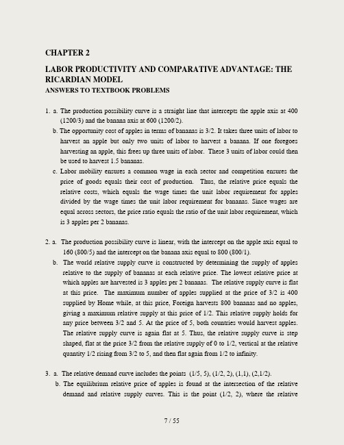
CHAPTER 2LABOR PRODUCTIVITY AND COMPARATIVE ADVANTAGE: THE RICARDIAN MODELANSWERS TO TEXTBOOK PROBLEMS1. a. The production possibility curve is a straight line that intercepts the apple axis at 400(1200/3) and the banana axis at 600 (1200/2).b. The opportunity cost of apples in terms of bananas is 3/2. It takes three units of labor toharvest an apple but only two units of labor to harvest a banana. If one foregoes harvesting an apple, this frees up three units of labor. These 3 units of labor could then be used to harvest 1.5 bananas.c. Labor mobility ensures a common wage in each sector and competition ensures theprice of goods equals their cost of production. Thus, the relative price equals the relative costs, which equals the wage times the unit labor requirement for apples divided by the wage times the unit labor requirement for bananas. Since wages are equal across sectors, the price ratio equals the ratio of the unit labor requirement, which is 3 apples per 2 bananas.2. a. The production possibility curve is linear, with the intercept on the apple axis equal to160 (800/5) and the intercept on the banana axis equal to 800 (800/1).b. The world relative supply curve is constructed by determining the supply of applesrelative to the supply of bananas at each relative price. The lowest relative price at which apples are harvested is 3 apples per 2 bananas. The relative supply curve is flat at this price. The maximum number of apples supplied at the price of 3/2 is 400 supplied by Home while, at this price, Foreign harvests 800 bananas and no apples, giving a maximum relative supply at this price of 1/2. This relative supply holds for any price between 3/2 and 5. At the price of 5, both countries would harvest apples.The relative supply curve is again flat at 5. Thus, the relative supply curve is step shaped, flat at the price 3/2 from the relative supply of 0 to 1/2, vertical at the relative quantity 1/2 rising from 3/2 to 5, and then flat again from 1/2 to infinity.3. a. The relative demand curve includes the points (1/5, 5), (1/2, 2), (1,1), (2,1/2).b. The equilibrium relative price of apples is found at the intersection of the relativedemand and relative supply curves. This is the point (1/2, 2), where the relativedemand curve intersects the vertical section of the relative supply curve. Thus the equilibrium relative price is 2.c. Home produces only apples, Foreign produces only bananas, and each country tradessome of its product for the product of the other country.d. In the absence of trade, Home could gain three bananas by foregoing two apples, andForeign could gain by one apple foregoing five bananas. Trade allows each country to trade two bananas for one apple. Home could then gain four bananas by foregoing two apples while Foreign could gain one apple by foregoing only two bananas. Each country is better off with trade.4. The increase in the number of workers at Home shifts out the relative supply schedulesuch that the corner points are at (1, 3/2) and (1, 5) instead of (1/2, 3/2) and (1/2, 5).The intersection of the relative demand and relative supply curves is now in the lower horizontal section, at the point (2/3, 3/2). In this case, Foreign still gains from trade but the opportunity cost of bananas in terms of apples for Home is the same whether or not there is trade, so Home neither gains nor loses from trade.5. This answer is identical to that in 3. The amount of "effective labor" has not changedsince the doubling of the labor force is accompanied by a halving of the productivity of labor.6. This statement is just an example of the pauper labor argument discussed in the chapter.The point is that relative wage rates do not come out of thin air; they are determined by comparative productivity and the relative demand for goods. The box in the chapter provides data which shows the strong connection between wages and productivity.Korea's low wage presumably reflects the fact that Korea is less productive than the United States in most industries. As the test example illustrated, a highly productive country that trades with a less productive, low-wage country will raise, not lower, its standard of living.7. The problem with this argument is that it does not use all the information needed fordetermining comparative advantage in production: this calculation involves the four unit labor requirements (for both the industry and service sectors, not just the two for the service sector). It is not enough to compare only service's unit labor requirements.If a ls< a ls*, Home labor is more efficient than foreign labor in services. While thisdemonstrates that the United States has an absolute advantage in services, this is neithera necessary nor a sufficient condition for determining comparative advantage. For thisdetermination, the industry ratios are also required. The competitive advantage of any industry depends on both the relative productivities of the industries and the relative wages across industries.8. While Japanese workers may earn the equivalent wages of U.S. workers, the purchasingpower of their income is one-third less. This implies that although w=w* (more or less), p<p* (since 3p=p*). Since the United States is considerably more productive in services, service prices are relatively low. This benefits and enhances U.S. purchasing power. However, many of these services cannot be transported and hence, are not traded. This implies that the Japanese may not benefit from the lower U.S. services costs, and do not face an international price which is lower than their domestic price.Likewise, the price of services in United States does not increase with the opening of trade since these services are non-traded. Consequently, U.S. purchasing power is higher than that of Japan due to its lower prices on non-traded goods.9. Gains from trade still exist in the presence of nontraded goods. The gains from tradedecline as the share of nontraded goods increases. In other words, the higher the portion of goods which do not enter international marketplace, the lower the potential gains from trade. If transport costs were high enough so that no goods were traded then, obviously, there would be no gains from trade.10. The world relative supply curve in this case consists of a step function, with as many"steps" (horizontal portions) as there are countries with different unit labor requirement ratios. Any countries to the left of the intersection of the relative demand and relative supply curves export the good in which they have a comparative advantage relative to any country to the right of the intersection. If the intersection occurs in a horizontal portion then the country with that price ratio produces both goods.CHAPTER 3SPECIFIC FACTORS AND INCOME DISTRIBUTIONANSWERS TO TEXTBOOK PROBLEMS1. Texas and Louisiana are states with large oil-producing sectors. The real wage of oil-producing factors of production in terms of other goods falls when the price of oil falls relative to the price of other goods. This was the source of economic decline in these states in 1986.2. To analyze the economy's production possibility frontier, consider how the output mixchanges as labor is shifted between the two sectors.a. The production functions for goods 1 and 2 are standard plots with quantities on the vertical axis, labor on the horizontal axis, and Q 1= Q 1(K 1,L 1) with slope equal to the MPL 1, and on another graph, Q 2= Q 2(K 2,L 2) with slope equal to the MPL 2.Q 1L 2 L 1PF 1 slope= -1 slope= -1/2100PF 2 PPF Q 1100 100Figure 3-1b. To graph the production possibilities frontier, combine the production function diagrams with the economy's allocation of labor in a four quadrant diagram. The economy's PPF is in the upper right hand corner, as is illustrated in the four quadrant diagram above. The PPF is curved due to declining marginal product of labor in each good.3. a. To solve this problem, one can graph the demand curve for labor in sector 1,represented by (w=MPL 1=demand for L 1) and the demand curve for labor in sector 2, represented by (w=MPL 2=demand for L 2) . Since the total supply of labor is given by the horizontal axis, the labor allocation between the sectors is approximately L 1=27 and L 2=73. The wage rate is approximately $0.98.Lw p 2xMPL 2p 1xMPL 1027100L 1L 2$1.00Figure 3-2b. Use the same type of graph as in problem 2b to show that sectoral output is Q 1=44 and Q 2=90. (This involves combining the production function diagrams with the economy's allocation of labor in a four quadrant diagram. The economy's PPF is in the upper right hand corner, as illustrated in the text.)c. Use a graph of labor demands, as in part a, to show that the intersection of the demand curves for labor occurs at a wage rate approximately equal to $0.74. The relative decline in the price of good 2 caused labor to be reallocated: labor is drawn out of production of good 2 and enters production of good 1 (L 1=62, L 2=38). This also leadsto an output adjustment, whereby production of good 2 falls to 68 units and production of good 1 rises to 76 units.d. With the relative price change from p 2/p 1=2 to p 2/p 1=1, the price of good 2 has fallen by 50 percent, while the price of good 1 has stayed the same. Wages have fallen, but by less than the fall in p 2 (wages fell approximately 25 percent). Thus, the real wage relative to p 2 actually rises while to real wage relative to p 1 falls. Hence, to determine the welfare consequences for workers, information is needed about their consumption shares of good 1 and good 2.4.The box diagram presented below is a useful tool for showing the effects of increasing the supply of the mobile factor of production, labor.a. For an economy producing two goods, X and Y, with labor demands reflected by their marginal revenue product curves, there is an initial wage of w 1 and an initial labor allocation of L x =O x A and L y =O y A. When the supply of labor increases, the right boundary of this diagram is pushed out to O y '. The demand for labor in sector Y is pulled rightward with the boundary. The new intersection of the labor demand curves shows that labor expands in both sectors, and therefore output of both X and Y also expand. The relative expansion of output is ambiguous. Wages paid to workers fall.O x A B 12 w 1P x MPL xw 2P y MPL y O y O y’Figure 3-3b. From the shape of the MPL curves, it is clear that labor will continue to exhibit diminishing returns. Using a four quadrant diagram, you can demonstrate that the new production possibility frontier is more concave and steeper (flatter) at the ends. Usingthe numerical example, L1increases to 90 from 62 and L2 increases to 50 from 38. Wages decline from $0.74 to $0.60. This new allocation of labor yields a new output mix of approximately Q1=85and Q2=77.CHAPTER 4RESOURCES AND TRADE: THE HECKSCHER-OHLIN MODEL ANSWERS TO TEXTBOOK PROBLEMS1. The definition of cattle growing as land intensive depends on the ratio of land to laborused in production, not on the ratio of land or labor to output. The ratio of land to labor in cattle exceeds the ratio in wheat in the United States, implying cattle is land intensive in the United States. Cattle is land intensive in other countries too if the ratio of land to labor in cattle production exceeds the ratio in wheat production in that country. Comparisons between another country and the United States is less relevant for this purpose.2. a. The box diagram has 600 as the length of two sides (representing labor) and 60 as thelength of the other two sides (representing land). There will be a ray from each of the two corners representing the origins. To find the slopes of these rays we use the information from the question concerning the ratios of the production coefficients.The question states that a LC / a TC = 20 and a LF / a TF = 5.Since a LC / a TC = (L C /Q C) / (T C /Q C) =L C /T C we have L C =20T C. Using the samereasoning, a LF / a TF = (L F /Q F) / (T F /Q F) =L F /T F and since this ratio equals 5, we have L F =5T F. We can solve this algebraically since L=L C+L F=600 and T=T C+T F=60.The solution is L C=400, T C=20, L F=200 and T F=40.b. The dimensions of the box change with each increase in available labor but the slopesof the rays from the origins remain the same. The solutions in the different cases are as follows.L=800: T C=33.33, L C=666.67, T F=26.67, L F=133.33L=1000: T C=46.67, L C=933.33, T F=13.33, L F=66.67L=1200: T C=60, L C=1200, T F=0, L F=0. (complete specialization).c. At constant factor prices, some labor would be unused, so factor prices would have tochange, or there would be unemployment.3. This question is similar to an issue discussed in Chapter 2. What matters is not theabsolute abundance of factors, but their relative abundance. Poor countries have an abundance of labor relative to capital when compared to more developed countries.4. In the Ricardian model, labor gains from trade through an increase in its purchasingpower. This result does not support labor union demands for limits on imports from less affluent countries. Labor may gain or lose from trade in the context of the Immobile Factors model. Purchasing power in terms of one good will rise, but in terms of the other good it will decline. The Heckscher-Ohlin model directly addresses distribution by considering the effects of trade on the owners of factors of production.In the context of this model, unskilled U.S. labor loses from trade since this group represents the relatively scarce factors in this country. The results from the Heckscher-Ohlin model support labor union demands for import limits.5. Conditions necessary for factor price equalization include both countries (or regions)produce both goods, both countries have the same technology of production, and the absence of barriers to trade. The difference between wages different regions of the United States may reflect all of these reasons; however, the barriers to trade are purely "natural" barriers due to transportation costs. U.S. trade with Mexico, by contrast, is also subject to legal limits; together with cultural differences that inhibit the flow of technology, this may explain why the difference in wage rates is so much larger.6. The factor proportions theory states that countries export those goods whoseproduction is intensive in factors with which they are abundantly endowed. One would expect the United States, which has a high capital/labor ratio relative to the rest of the world, to export capital-intensive goods if the Heckscher-Ohlin theory holds. Leontief found that the United States exported labor-intensive goods. Bowen, Leamer and Sveikauskas found for the world as a whole the correlation between factor endowment and trade patterns to be tenuous. The data do not support the predictions of the theory that countries' exports and imports reflect the relative endowments of factors.7. If the efficiency of the factors of production differ internationally, the lessons of theHeckscher-Ohlin theory would be applied to “effective factors” which adjust for the differences in technology or worker skills or land quality (for example). The adjusted model has been found to be more successful than the unadjusted model at explaining the pattern of trade between countries. Factor-price equalization concepts would applyto the effective factors. A worker with more skills or in a country with better technology could be considered to be equal to two workers in another country. Thus, the single person would be two effective units of labor. Thus, the one high-skilled worker could earn twice what lower skilled workers do and the price of one effective unit of labor would still be equalized.CHAPTER 5THE STANDARD TRADE MODELANSWERS TO TEXTBOOK PROBLEMS1. An increase in the terms of trade increases welfare when the PPF is right-angled. Theproduction point is the corner of the PPF. The consumption point is the tangency of the relative price line and the highest indifference curve. An improvement in the terms of trade rotates the relative price line about its intercept with the PPF rectangle (since there is no substitution of immobile factors, the production point stays fixed). The economy can then reach a higher indifference curve. Intuitively, although there is no supply response, the economy receives more for the exports it supplies and pays less for the imports it purchases.2. The difference from the standard diagram is that the indifference curves are rightangles rather than smooth curves. Here, a terms of trade increase enables an economy to move to a higher indifference curve. The income expansion path for this economy is a ray from the origin. A terms of trade improvement moves the consumption point further out along the ray.3. The terms of trade of Japan, a manufactures (M) exporter and a raw materials (R)importer, is the world relative price of manufactures in terms of raw materials (p M/p R).The terms of trade change can be determined by the shifts in the world relative supply and demand (manufactures relative to raw materials) curves. Note that in the following answers, world relative supply (RS) and relative demand (RD) are always M relative to R. We consider all countries to be large, such that changes affect the world relative price.a. Oil supply disruption from the Middle East decreases the supply of raw materials,which increases the world relative supply. The world relative supply curve shifts out, decreasing the world relative price of manufactured goods and deteriorating Japan's terms of trade.b. Korea’s increased automobile production increases the supply of manufactures, whichincreases the world RS. The world relative supply curve shifts out, decreasing the world relative price of manufactured goods and deteriorating Japan's terms of trade.c. U.S. development of a substitute for fossil fuel decreases the demand for raw materials.This increases world RD and the world relative demand curve shifts out, increasing theworld relative price of manufactured goods and improving Japan's terms of trade. This occurs even if no fusion reactors are installed in Japan since world demand for raw materials falls.d. A harvest failure in Russia decreases the supply of raw materials, which increases theworld RS. The world relativ e supply curve shifts out. Also, Russia’s demand for manufactures decreases, which reduces world demand so that the world relative demand curve shifts in. These forces decrease the world relative price of manufactured goods and deteriorate Japan's terms of trade.e. A reduction in Japan’s tariff on raw materials will raise its internal relative price ofmanufactures. This price change will increase Japan’s RS and decrease Japan’s RD, which increases the world RS and decreases the world RD (i.e., world RS shifts out and world RD shifts in). The world relative price of manufactures declines and Japan’s terms of trade deteriorate.4. These results acknowledge the biased growth which occurs when there is an increasein one factor of production. An increase in the capital stock of either country favors production of good X while an increase in the labor supply favors production of good Y. Also, recognize the Heckscher-Ohlin result that an economy will export that good which uses intensively the factor which hat economy has in relative abundance.Country A exports good X to country B and imports good Y from country B. The possibility of immiserizing growth makes the welfare effects of a terms of trade improvement due to export-biased growth ambiguous. Import-biased growth unambiguously improves welfare for the growing country.a. A's terms of trade worsen, A's welfare may increase or, less likely, decrease, and B'swelfare increases.b. A's terms of trade improve, A's welfare increases and B's welfare decreases.c. B's terms of trade improve, B's welfare increases and A's welfare decreases.d. B's terms of trade worsen, B's welfare may increase or, less likely, decrease, and A'swelfare increases.5. Immiserizing growth occurs when the welfare deteriorating effects of a worsening inan economy's terms of trade swamp the welfare improving effects of growth. For this to occur, an economy must undergo very biased growth and the economy must be a large enough actor in the world economy such that its actions spill over to adversely alter the terms of trade to a large degree. This combination of events is unlikely to occur in practice.6. Aid which must be spent on exports increases the demand for those export goods andraises their price relative to other goods. There will be a terms of trade deterioration for the recipient country. This can be viewed as a polar case of the effect of a transfer on the terms of trade. Here, the marginal propensity to consume the export good by the recipient country is 1. The donor benefits from a terms of trade improvement. As with immiserizing growth, it is theoretically possible that a transfer actually worsens the welfare of the recipient.7. Given the difference in technological development between most Eastern Europeancountries and the United States and Japan, the effects on Western European prices will depend, in the short run, on transfer problem issues and, in the long run, on the likely biases in Eastern Europe's growth. The transfer problem point is concerned with the consumption demands of countries which receive available international credit supplies. If loans to developing countries shift from availability to Latin American countries, which have a relatively high propensity to consume U.S. goods, to availability to Eastern European countries, which have a lower propensity to consume U.S. goods and a higher propensity to consume German goods, the price of German exports will rise relative to the price of U.S. exports. This would lead to an improvement in the terms of trade of Germany and a worsening of the terms of trade of the United States. Note, however, that in the long term, the analysis of terms of trade effects should also consider whether the biases in economic growth in Eastern Europe will be in sectors of the economy more closely aligned with the export industries of Germany or of the United States. The greater the similarity of the export-oriented industrial push in Eastern European with the existing industries in Germany, the greater the supply side reversal of the favorable German terms of trade movement which had arisen from the demand side forces of the transfer problem.8. When a country subsidizes its exports, the world relative supply and relative demandschedules shift such that the terms of trade for the country worsen. A countervailing import tariff in a second country exacerbates this effect, moving the terms of trade even further against the first country. The first country is worse off both because of the deterioration of the terms of trade and the distortions introduced by the new internal relative prices. The second country definitely gains from the first country's export subsidy, and may gain further from its own tariff. If the second country retaliated with an export subsidy then this would offset the initial improvement in theterms of trade; the "retaliatory" export subsidy definitely helps the first country and hurts the second.CHAPTER 6ECONOMIES OF SCALE, IMPERFECT COMPETITION, AND INTERNATIONAL TRADEANSWERS TO TEXTBOOK PROBLEMS1. Cases a and d reflect external economies of scale since concentration of the productionof an industry in a few locations reduces the industry's costs even when the scale of operation of individual firms remains small. External economies need not lead to imperfect competition. The benefits of geographical concentration may include a greater variety of specialized services to support industry operations and larger labor markets or thicker input markets. Cases b and c reflect internal economies of scale and occur at the level of the individual firm. The larger the output of a product by a particular firm, the lower its average costs. This leads to imperfect competition as in petrochemicals, aircraft, and autos.2. The profit maximizing output level of a monopolist occurs where marginal revenueequals marginal cost. Unlike the case of perfectly competitive markets, under monopoly marginal revenue is not equal to price. Marginal revenue is always less than price under imperfectly competitive markets because to sell an extra unit of output the firm must lower the price of all units, not just the marginal one.3. By concentrating the production of each good with economies of scale in one countryrather than spreading the production over several countries, the world economy will use the same amount of labor to produce more output. In the monopolistic competition model, such a concentration of labor benefits the host country, which can also capture some monopoly rents, while it may hurt the rest of the world which could then face higher prices on its consumption goods. In the external economies case, such monopolistic pricing behavior is less likely since imperfectly competitive markets are less likely.4. Although this problem is a bit tricky and the numbers don't work out nicely, a solutiondoes exist. The first step in finding the solution is to determine the equilibrium number of firms in the industry. The equilibrium number of firms is that number, n, at whichprice equals average cost. We know that AC=F/X + c , where F represents fixed costs of production, X represents the level of sales by each firm, and c represents marginal costs. We also know that P=c+ (1/bn), where P and b represent price and the demand parameter. Also, if all firms follow the same pricing rule, then X=S/n where S equals total industry sales. So, set price equal to average cost, cancel out the c's and replace X by S/n. Rearranging what is left yields the formula n2=S/Fb. Substitute in S=900,000+ 1,600,000+ 3,750,000 =6,250,000, F=750,000,000 and b=1/30,000. The numerical answer is that n=15.8 firms. However, since you will never see .8 firms, there will be15 firms that enter the market, not 16 firms since the last firm knows that it can notmake positive profits. The rest of the solution is straight-forward. Using X=S/n, output per firm is 41,666 units. Using the price equation, and the fact that c=5,000, yields an equilibrium price of $7,000.5. a. The relatively few locations for production suggest external economies of scale inproduction. If these operations are large, there may also be large internal economies of scale in production.b. Since economies of scale are significant in airplane production, it tends to be done by asmall number of (imperfectly competitive) firms at a limited number of locations. One such location is Seattle, where Boeing produces.c. Since external economies of scale are significant in semiconductor production,semiconductor industries tend to be concentrated in certain geographic locations. If, for some historical reason, a semiconductor is established in a specific location, the export of semiconductors by that country is due to economies of scale and not comparative advantage.d. "True" scotch whiskey can only come from Scotland. The production of scotchwhiskey requires a technique known to skilled distillers who are concentrated in the region. Also, soil and climactic conditions are favorable for grains used in local scotch production. This reflects comparative advantage.e. France has a particular blend of climactic conditions and land that is difficult toreproduce elsewhere. This generates a comparative advantage in wine production.6. The Japanese producers are price discriminating across United States and Japanesemarkets, so that the goods sold in the United States are much cheaper than those sold in Japan. It may be profitable for other Japanese to purchase these goods in the United States, incur any tariffs and transportation costs, and resell the goods in Japan. Clearly, the price differential across markets must be non-trivial for this to be profitable.。
克鲁格曼 国际经济学第10版 英文答案 国际贸易部分krugman_intlecon10_im_12_GE
Chapter 12Controversies in Trade Policy⏹Chapter OrganizationSophisticated Arguments for Activist Trade PolicyTechnology and ExternalitiesImperfect Competition and Strategic Trade PolicyBox: A Warning from Intel’s FounderCase Study: When the Chips Were UpGlobalization and Low-Wage LaborThe Anti-Globalization MovementTrade and Wages RevisitedLabor Standards and Trade NegotiationsEnvironmental and Cultural IssuesThe WTO and National IndependenceCase Study: A Tragedy in BangladeshGlobalization and the EnvironmentGlobalization, Growth, and PollutionThe Problem of “Pollution Havens”The Carbon Tariff DisputeSummary⏹Chapter OverviewAlthough the text has shown why, in general, free trade is a good policy, this chapter considers two controversies in trade policy that challenge free trade. The first regards strategic trade policy. Proponents of activist government trade intervention argue that certain industries are desirable and may be underfunded by markets or dominated by imperfect competition and warrant some government intervention. The second controversy regards the recent debate over the effects of globalization on workers, the environment, and sovereignty. While the anti-globalization arguments often lack sound structure, their visceral nature demonstrates that the spread of trade is extremely troubling to some groups.As seen in the previous chapters, activist trade policy may be justified if there are market failures. One important type of market failure involves externalities present in high-technology industries due to their knowledge creation. Existence of externalities associated with research and development and high technology make the private return to investing in these activities less than their social return. This means© 2015 Pearson Education, Inc.64 Krugman/Obstfeld/Melitz •International Economics: Theory & Policy, Tenth Editionthat the private sector will tend to invest less in high-technology sectors than is socially optimal. Although there may be some case for intervention, the difficulties in targeting the correct industry and understanding the quantitative size of the externality make effective intervention complicated. To address this market failure of insufficient knowledge creation, the first best policy may be to directly support research and development in all industries. Still, although it is a judgment call, the technology spillover case for industrial policy probably has better footing in solid economics than any other argument.Another set of market failures arises when imperfect competition exists. Strategic trade policy by a government can work to deter investment and production by foreign firms and raise the profits of domestic firms.An example is provided in the text that illustrates the case where the increase in profits following the imposition of a subsidy can actually exceed the cost of a subsidy to an imperfectly competitive industryif domestic firms can capture profits from foreign firms. Although this is a valid theoretical argument for strategic policy, it is nonetheless open to criticism in choosing the industries that should be subsidized and the levels of subsidies to these industries. These criticisms are associated with the practical aspects of insufficient information and the threat of foreign retaliation. The case study on the attempts to promote the semiconductor chips industry shows that neither excess returns nor knowledge spillovers necessarily materialize even in industries that seem perfect for activist trade policy.The next section of the chapter examines the anti-globalization movement. In particular, it examines the concerns over low wages in poor countries. Standard analysis suggests that trade should help poor countries and, in particular, help the abundant factor (labor) in those countries. Protests in Seattle, which shut down WTO negotiations, and subsequent demonstrations at other meetings showed, though, that protestors either did not understand or did not agree with this analysis.The concern over low wages in poor countries is a revision of arguments in Chapter 2. Analysis in the current chapter shows again that trade should help the purchasing power of all workers and that if anyone is hurt, it is the workers in labor-scarce countries. The low wages in export sectors of poor countriesare higher than they would be without the export-oriented manufacturing, and although the situation of these workers may be more visible than before, that does not make it worse. Practically, the policy issue is whether or not labor standards should be part of trade pacts. Although such standards may act in ways similar to a domestic minimum wage, developing countries fear that such standards would be used as a protectionist tool. A case study on the 2013 collapse of a garment factory in Bangladesh highlights this tension. The Bangladeshi garment industry would not be globally competitive if it had to raise labor standards to rich country standards. Bangladeshi garment workers, though very poorly paid by rich country standards, earn more than workers in non-export sectors. A potential solution would be for consumers in rich countries to pay more for goods certified to have been produced under improved labor standards, thereby giving producers in poor countries both the means and the incentive to improve labor standards,Anti-globalization protestors were by no means united in their cause. There were also strong concerns that export manufacturing in developing countries was bad for the environment. Again, the issue is whether these concerns should be addressed by tying environmental standards into trade negotiations, and the open question is whether this can be done without destroying the export industries in developing countries. Globalization raises questions of cultural independence and national sovereignty. Specifically, many countries are disturbed by the WTO’s ability to overturn laws that do not seem to be trade restrictions but which nonetheless have trade impacts. This point highlights the difficulty of advancing trade liberalization when the clear impediments to trade—tariffs or quotas—have been removed, yet national policies regarding industry promotion or labor and environmental standards still need to be reformed.© 2015 Pearson Education LimitedThe final section of the chapter examines the link between trade and the environment. In general, production and consumption can cause environmental damage. Yet, as a country’s GDP per capita grows, the environmental damage done first grows and then eventually declines as the country gets rich enough to begin to protect the environment. As trade has lifted incomes of some countries, it may have been bad for the environment—but largely by making poor countries richer, an otherwise good thing. In theory, there could be a concern about “pollution havens,” that is countries with low environmental standards that attract “dirty” industries. There is relatively little evidence of this ph enomenon thus far. Furthermore, the pollution in these locations tends to be localized and is therefore better left to national rather than international policy. The chapter concludes with a discussion of the cap and trade system for greenhouse gases (an example of transboundary pollution) currently being debated in the U.S. Congress. Part of this policy aimed at reducing carbon emissions is an imposition of a “carbon tariff” on imports from countries that do not have their own carbon taxes. Proponents argue that such tariffs are necessary to prevent production from shifting to pollution havens and to reduce the overall level of carbon emissions, while opponents argue that these tariffs are simply more protectionism masquerading as environmental regulation.Answers to Textbook Problems1. The main disadvantage is that strategic trade policy can lead to both “rent-seeking” and beggar-thy-neighbor policies, which can increase one country’s welfare at the other country’s expense. Such policies can lead to a trade war in which every country is worse off, even though one country could become better off in the absence of retaliation. This is the danger in enacting strategic trade policy: It often provokes retaliation, which, in the long run, can make everyone worse off. Furthermore, it can be difficult to identify both which industries to subsidize and how much to subsidize them. Failure to correctly identify these factors can lead to a net loss from a subsidy.2. Globalization has many pros and cons, well-illustrated in famous controversies—like the onestimulated by Joseph Stiglitz’s book, Globalization and Its Discontents. Initiatives like the Doha Development Agenda try to address some of them and find solutions acceptable to every country. 3. The results of basic research may be appropriated by a wider range of firms and industries thanthe results of research applied to specific industrial applications. The benefits to the United States of Japanese basic research would exceed the benefits from Japanese research targeted to specific problems in Japanese industries. A specific application may benefit just one firm in Japan, perhaps simply subsidizing an activity that the market is capable of funding. General research will provide benefits that spill across borders to many firms and may be countering a market failure, externalities present in the advancement of general knowledge.4. The reason why strategic trade policies attract retaliation from other countries is because they presentthe same problems that are faced when considering the use of a tariff to improve the terms of trade.Strategic policies are, in essence, a type of beggar-thy-neighbor policies that increase one country’s welfare at other countries’ expense. A good example is represented by export quot as on scarcemineral ores—like the one adopted by China for Rare Earth Elements (REE) exports since 2006—that have already provoked filing a complaint to the WTO by the US, the EU, and Japan.。
克鲁格曼《国际经济学》第八版课后答案(英文)-Ch08
Chapter 8The Instruments of Trade PolicyChapter OrganizationBasic Tariff AnalysisSupply, Demand, and Trade in a Single IndustryEffects of a TariffMeasuring the Amount of ProtectionCosts and Benefits of a TariffConsumer and Producer SurplusMeasuring the Costs and BenefitsOther Instruments of Trade PolicyExport Subsidies: TheoryCase Study: Europe’s Common Agricultural PolicyImport Quotas: TheoryCase Study: An Import Quota in Practice: U.S. SugarVoluntary Export RestraintsCase Study: A Voluntary Export Restraint in Practice: Japanese Autos Local Content RequirementsBox: American Buses, Made in HungaryOther Trade Policy InstrumentsThe Effects of Trade Policy: A SummarySummaryAppendix I: Tariff Analysis in General EquilibriumA Tariff in a Small CountryA Tariff in a Large CountryAppendix II: Tariffs and Import Quotas in the Presence of Monopoly The Model with Free TradeThe Model with a TariffThe Model with an Import QuotaComparing a Tariff with a QuotaChapter 8 The Instruments of Trade Policy 33Chapter OverviewThis chapter and the next three focus on international trade policy. Students will have heard various arguments for and against restrictive trade practices in the media. Some of these arguments are sound and some are clearly not grounded in fact. This chapter provides a framework for analyzing the economic effects of trade policies by describing the tools of trade policy and analyzing their effects on consumers and producers in domestic and foreign countries. Case studies discuss actual episodes of restrictive trade practices. An instructor might try to underscore the relevance of these issues by having students scan newspapers and magazines for other timely examples of protectionism at work.The analysis presented here takes a partial equilibrium view, focusing on demand and supply in one market, rather than the general equilibrium approach followed in previous chapters. Import demand and export supply curves are derived from domestic and foreign demand and supply curves. There are a number of trade policy instruments analyzed in this chapter using these tools. Some of the important instruments of trade policy include specific tariffs, defined as taxes levied as a fixed charge for each unit of a good imported; ad valorem tariffs, levied as a fraction of the value of the imported good; export subsidies, which are payments given to a firm or industry that ships a good abroad; import quotas, which are direct restrictions on the quantity of some good that may be imported; voluntary export restraints, which are quotas on trading that are imposed by the exporting country instead of the importing country; and local content requirements, which are regulations that require that some specified fraction of a good is produced domestically.The import supply and export demand analysis demonstrates that the imposition of a tariff drives a wedge between prices in domestic and foreign markets, and increases prices in the country imposing the tariff and lowers the price in the other country by less than the amount of the tariff. This contrasts with most textbook presentations which make the small country assumption that the domestic internal price equals the world price times one plus the tariff rate. The actual protection provided by a tariff willnot equal the tariff rate if imported intermediate goods are used in the production of the protected good. The proper measurement, the effective rate of protection, is described in the text and calculated for a sample problem.The analysis of the costs and benefits of trade restrictions require tools of welfare analysis. The text explains the essential tools of consumer and producer surplus. Consumer surplus on each unit sold is defined as the difference between the actual price and the amount that consumers would have been willing to pay for the product. Geometrically, consumer surplus is equal to the area under the demand curve and above the price of the good. Producer surplus is the difference between the minimum amount for which a producer is willing to sell his product and the price which he actually receives. Geometrically, producer surplus is equal to the area above the supply curve and below the price line. These tools are fundamental to the student’s understanding of the implications of trade polici es and should be developed carefully. The costs of a tariff include distortionary efficiency losses in both consumption and production. A tariff provides gains from terms of trade improvement when and if it lowers the foreign export price. Summing the areas in a diagram of internal demand and supply provides a method for analyzing the net loss or gain from a tariff.Other instruments of trade policy can be analyzed with this method. An export subsidy operates in exactly the reverse fashion of an import tariff. An import quota has similar effects as an import tariff upon prices and quantities, but revenues, in the form of quota rents, accrue to foreign producers of the protected good. Voluntary export restraints are a form of quotas in which import licenses are held by foreign governments. Local content requirements raise the price of imports and domestic goods and do not result in either government revenue or quota rents.34 Krugman/Obstfeld •International Economics: Theory and Policy, Eighth EditionThroughout the chapter the analysis of different trade restrictions are illustrated by drawing upon specific episodes. Europe’s common agricultural policy provides and example of export subsidies in action. The case study corresponding to quotas describes trade restrictions on U.S. sugar imports. Voluntary export restraints are discussed in the context of Japanese auto sales to the United States. The oil import quota in the United States in the 1960’s provides an example of a local content scheme.There are two appendices to this chapter. Appendix I uses a general equilibrium framework to analyze the impact of a tariff, departing from the partial equilibrium approach taken in the chapter. When a small country imposes a tariff, it shifts production away from its exported good and toward the imported good. Consumption shifts toward the domestically produced goods. Both the volume of trade and welfare of the country decline. A large country imposing a tariff can improve its terms of trade by an amount potentially large enough to offset the production and consumption distortions. For a large country, a tariff may be welfare improving.Appendix II discusses tariffs and import quotas in the presence of a domestic monopoly. Free trade eliminates the monopoly power of a domestic producer and the monopolist mimics the actions of a firm in a perfectly competitive market, setting output such that marginal cost equals world price. A tariff raises domestic price. The monopolist, still facing a perfectly elastic demand curve, sets output such that marginal cost equals internal price. A monopolist faces a downward sloping demand curve under a quota.A quota is not equivalent to a tariff in this case. Domestic production is lower and internal price higher when a particular level of imports is obtained through the imposition of a quota rather than a tariff.Answers to Textbook Problems1. The import demand equation, MD, is found by subtracting the home supply equation from the homedemand equation. This results in MD= 80 - 40 ⨯P. Without trade, domestic prices and quantities adjust such that import demand is zero. Thus, the price in the absence of trade is 2.2. a. Foreign’s export supply curve, XS, is XS=-40 + 40⨯P. In the absence of trade, the price is 1.b. When trade occurs, export supply is equal to import demand, XS=MD. Thus, using theequations from Problems 1 and 2a, P= 1.50, and the volume of trade is 20.3. a. The new MD curve is 80 - 40 ⨯ (P+ t) where t is the specific tariff rate, equal to 0.5. (Note: Insolving these problems, you should be careful about whether a specific tariff or ad valorem tariff is imposed. With an ad valorem tariff, the MD equation would be expressed as MD= 80 - 40 ⨯(1 + t)P.) The equation for the export supply curve by the foreign country is unchanged. Solving,we find that the world price is $1.25, and thus the internal price at home is $1.75. The volume of trade has been reduced to 10, and the total demand for wheat at home has fallen to 65 (from thefree trade level of 70). The total demand for wheat in Foreign has gone up from 50 to 55.b. andc. The welfare of the home country is best studied using the combined numerical andgraphical solutions presented below in Figure 8.1.Figure 8.1Chapter 8 The Instruments of Trade Policy 35where the areas in the figure are:a.55(1.75 - 1.50) -0.5(55 - 50)(1.75 - 1.50) = 13.125b. 0.5(55 - 50)(1.75 - 1.50) = 0.625c. (65 - 55)(1.75 - 1.50) = 2.50d. 0.5(70 - 65)(1.75 - 1.50) = 0.625e. (65 - 55)(1.50 - 1.25) = 2.50Consumer surplus change: -(a+ b+ c+ d) =-16.875. Producer surplus change: a= 13.125.Government revenue change: c+ e= 5. Efficiency losses b+ d are exceeded by terms of tradegain e. (Note: In the calculations for the a, b, and d areas, a figure of 0.5 shows up. This isbecause we are measuring the area of a triangle, which is one-half of the area of the rectangledefined by the product of the horizontal and vertical sides.)4. Using the same solution methodology as in Problem 3, when the home country is very small relativeto the foreign country, its effects on the terms of trade are expected to be much less. The smallcountry is much more likely to be hurt by its imposition of a tariff. Indeed, this intuition is shown in this problem. The free trade equilibrium is now at the price $1.09 and the trade volume is now$36.40.With the imposition of a tariff of 0.5 by Home, the new world price is $1.045, the internal home price is $1.545, home demand is 69.10 units, home supply is 50.90, and the volume of trade is 18.20.When Home is relatively small, the effect of a tariff on world price is smaller than when Home is relatively large. When Foreign and Home were closer in size, a tariff of 0.5 by home lowered world price by 25 percent, whereas in this case the same tariff lowers world price by about 5 percent. The internal Home price is now closer to the free trade price plus t than when Home was relatively large.In this case, the government revenues from the tariff equal 9.10, the consumer surplus loss is 33.51, and the producer surplus gain is 21.089. The distortionary losses associated with the tariff (areas b+ d) sum to 4.14 and the terms of trade gain (e) is 0.819. Clearly, in this small country example, the distortionary losses from the tariff swamp the terms of trade gains. The general lesson is the smaller the economy, the larger the losses from a tariff since the terms of trade gains are smaller.5. ERP = (200 ⨯ 1.50 - 200)/100 = 100%6. The effective rate of protection takes into consideration the costs of imported intermediate goods.Here, 55% of the cost can be imported, suggesting with no distortion, home value added would be 45%. A 15% increase in the price of ethanol, though, means home value added could be as high as 60%. Effective rate of protection = (V t-V w)/V w, where V t is the value added in the presence of trade policies, and V w is the value added without trade distortions. In this case, we have (60 - 45)/45 = 33% effective rate of protection.7. We first use the foreign export supply and domestic import demand curves to determine the newworld price. The foreign supply of exports curve, with a foreign subsidy of 50 percent per unit,becomes XS=-40 + 40(1 + 0.5) ⨯P. The equilibrium world price is 1.2 and the internal foreign price is 1.8. The volume of trade is 32. The foreign demand and supply curves are used to determine the costs and benefits of the subsidy. Construct a diagram similar to that in the text and calculate the area of the various polygons. The government must provide (1.8 - 1.2)⨯ 32 = 19.2 units of output to support the subsidy. Foreign producers surplus rises due to the subsidy by the amount of 15.3 units of output. Foreign consumers surplus falls due to the higher price by 7.5 units of the good. Thus, the net loss to Foreign due to the subsidy is 7.5 + 19.2 - 15.3 = 11.4 units of output. Home consumers and producers face an internal price of 1.2 as a result of the subsidy. Home consumers surplus rises by 70 ⨯ 0.3 + 0.5 (6⨯ 0.3) = 21.9, while Home producers surplus falls by 44 ⨯ 0.3 + 0.5(6 ⨯ 0.3) =14.1, for a net gain of 7.8 units of output.36 Krugman/Obstfeld •International Economics: Theory and Policy, Eighth Edition8. a. False, unemployment has more to do with labor market issues and the business cycle than withtariff policy.b. False, the opposite is true because tariffs by large countries can actually reduce world priceswhich helps offset their effects on consumers.c. This kind of policy might reduce automobile production and Mexico, but also would increase theprice of automobiles in the United States, and would result in the same welfare loss associatedwith any quota.9. At a price of $10 per bag of peanuts, Acirema imports 200 bags of peanuts. A quota limiting theimport of peanuts to 50 bags has the following effects:a. The price of peanuts rises to $20 per bag.b. The quota rents are ($20 - $10) ⨯ 50 = $500.c. The consumption distortion loss is 0.5 ⨯ 100 bags ⨯ $10 per bag = $500.d. The production distortion loss is 0.5 ⨯ 50 bags ⨯ $10 per bag = $250.10. The reason is largely that the benefits of these policies accrue to a small group of people and thecosts are spread out over many people. Thus, those that benefit care far more deeply about these policies. These typical political economy problems associated with trade policy are probably even more troublesome in agriculture, where there are long standing cultural reasons for farmers andfarming communities to want to hold onto their way of life, making the interests even moreentrenched than they would normally be.11. It would improve the income distribution within the economy since wages in manufacturing wouldincrease, and real incomes for others in the economy would decrease due to higher prices formanufactured goods. This is true only under the assumption that manufacturing wages are lower than all others in the economy. If they were higher than others in the economy, the tariff policies would worsen the income distribution.。
克鲁格曼 国际经济学第10版 英文答案 国际金融部分krugman_intlecon10_im_14_GE
Chapter 14 (3)Exchange Rates and the Foreign Exchange Market: An Asset ApproachChapter OrganizationExchange Rates and International TransactionsDomestic and Foreign PricesExchange Rates and Relative PricesThe Foreign Exchange MarketThe ActorsBox: Exchange Rates, Auto Prices, and Currency WarsCharacteristics of the MarketSpot Rates and Forward RatesForeign Exchange SwapsFutures and OptionsThe Demand for Foreign Currency AssetsAssets and Asset ReturnsBox: Nondeliverable Forward Exchange Trading in AsiaRisk and LiquidityInterest RatesExchange Rates and Asset ReturnsA Simple RuleReturn, Risk, and Liquidity in the Foreign Exchange MarketEquilibrium in the Foreign Exchange MarketInterest Parity: The Basic Equilibrium ConditionHow Changes in the Current Exchange Rate Affect Expected ReturnsThe Equilibrium Exchange RateInterest Rates, Expectations, and EquilibriumThe Effect of Changing Interest Rates on the Current Exchange RateThe Effect of Changing Expectations on the Current Exchange RateCase Study: What Explains the Carry Trade?SummaryAPPENDIX TO CHAPTER 14 (3): Forward Exchange Rates and Covered Interest Parity© 2015 Pearson Education LimitedChapter OverviewThe purpose of this chapter is to show the importance of the exchange rate in translating foreign prices into domestic values as well as to begin the presentation of exchange rate determination. Central to the treatment of exchange rate determination is the insight that exchange rates are determined in the same way a s other asset prices. The chapter begins by describing how the relative prices of different countries’ goods are affected by exchange rate changes. This discussion illustrates the central importance of exchange rates for cross-border economic linkages. The determination of the level of the exchange rate is modeled in the context of the exchange rate’s role as the relative price of foreign and domestic currencies, using the uncovered interest parity relationship.The euro is used often in examples. Some students may not be familiar with the currency or aware of which countries use it; a brief discussion may be warranted. A full treatment of EMU and the theories surrounding currency unification appears in Chapter 20(9).The description of the foreign exchange market stresses the involvement of large organizations (commercial banks, corporations, nonbank financial institutions, and central banks) and the highly integrated natureof the market. The nature of the foreign exchange market ensures that arbitrage occurs quickly so that common rates are offered worldwide. A comparison of the trading volume in foreign exchange markets to that in other markets is useful to underscore how quickly price arbitrage occurs and equilibrium is restored. Forward foreign exchange trading, foreign exchange futures contracts, and foreign exchange options play an important part in currency market activity. The use of these financial instruments to eliminate short-run exchange rate risk is described.The explanation of exchange rate determination in this chapter emphasizes the modern view that exchange rates move to equilibrate asset markets. The foreign exchange demand and supply curves that introduce exchange rate determination in most undergraduate texts are not found here. Instead, there is a discussion of asset pricing and the determination of expected rates of return on assets denominated in different currencies.Students may already be familiar with the distinction between real and nominal returns. The text demonstrates that nominal returns are sufficient for comparing the attractiveness of different assets. There is a brief description of the role played by risk and liquidity in asset demand, but these considerations are not pursued in this chapter. (The role of risk is taken up again in Chapter 18[7].)Substantial space is devoted to the topic of comparing expected returns on assets denominated in domestic and foreign currency. The text identifies two parts of the expected return on a foreign currency asset (measured in domestic currency terms): the interest payment and the change in the value of the foreign currency relative to the domestic currency over the period in which the asset is held. The expected return on a foreign asset is calculated as a function of the current exchange rate for given expected values of the future exchange rate and the foreign interest rate.The absence of risk and liquidity considerations implies that the expected returns on all assets traded in the foreign exchange market must be equal. It is thus a short step from calculations of expected returns on foreign assets to the interest parity condition. The foreign exchange market is shown to be in equilibrium only when the interest parity condition holds. Thus, for given interest rates and given expectations about future exchange rates, interest parity determines the current equilibrium exchange rate. The interest parity diagram introduced here is instrumental in later chapters in which a more general model is presented. Because a command of this interest parity diagram is an important building block for future work, we recommend drills that employ this diagram.The result that a dollar appreciation makes foreign currency assets more attractive may appear counterintuitive to students—why does a stronger dollar reduce the expected return on dollar assets? The key to explaining this point is that, under the static expectations and constant interest rates assumptions, a dollar appreciation today implies a greater future dollar depreciation; so, an American investor can expect to gain not only theChapter 14Exchange Rates and the Foreign Exchange Market: An Asset Approach 77© 2015 Pearson Education Limitedforeign interest payment but also the extra return due to the dollar’s additional future depreciation. The following diagram illustrates this point. In this diagram, the exchange rate at time t + 1 is expected to be equal to E . If the exchange rate at time t is also E , then expected depreciation is 0. If, however, the exchange rate depreciates at time t to E ', then it must appreciate to reach E at time t + 1. If the exchange rate appreciates today to E ", then it must depreciate to reach E at time t + 1. Thus, under static expectations, a depreciation today implies an expected appreciation and vice versa.Figure 14(3)-1This pedagogical tool can be employed to provide some further intuition behind the interest parityrelationship. Suppose that the domestic and foreign interest rates are equal. Interest parity then requires that the expected depreciation is equal to zero and that the exchange rate today and next period is equal to E . If the domestic interest rate rises, people will want to hold more domestic currency deposits. The resulting increased demand for domestic currency drives up the price of domestic currency, causing the exchange rate to appreciate. How long will this continue? The answer is that the appreciation of the domestic currency continues until the expected depreciation that is a consequence of the domestic currency’s appreciation today just offsets the interest differential.The text presents exercises on the effects of changes in interest rates and of changes in expectations of the future exchange rate. These exercises can help develop students’ intuition. For example, the initial result of a rise in U.S. interest rates is a higher demand for dollar-denominated assets and thus an increase in the price of the dollar. This dollar appreciation is large enough that the subsequent expected dollar depreciation just equalizes the expected return on foreign currency assets (measured in dollar terms) and the higher dollar interest rate.The chapter concludes with a case study looking at a situation in which interest rate parity may not hold: the carry trade. In a carry trade, investors borrow money in low-interest currencies and buy high-interest-rate currencies, often earning profits over long periods of time. However, this transaction carries an element of risk as the high-interest-rate currency may experience an abrupt crash in value. The case study discusses a popular carry trade in which investors borrowed low-interest-rate Japanese yen to purchase high-interest-rate Australian dollars. Investors earned high returns until 2008, when the Australian dollar abruptly crashed, losing 40 percent of its value. This was an especially large loss as the crash occurred amidst a financial crisis in which liquidity was highly valued. Thus, when we factor in this additional risk of the carry trade, interest rate parity may still hold.The Appendix describes the covered interest parity relationship and applies it to explain the determination of forward rates under risk neutrality as well as the high correlation between movements in spot and forward rates.Answers to Textbook Problems1. At an exchange rate of 1.05 $ per euro, a 5 euro bratwurst costs 1.05$/euro ⨯ 5 euros = $5.25. Thus,the bratwurst in Munich is $1.25 more expensive than the hot dog in Boston. The relative price is $5.25/$4 = 1.31. A bratwurst costs 1.31 hot dogs. If the dollar depreciates to 1.25$/euro, the bratwurst now costs 1.25$/euro ⨯ 5 euros = $6.25, for a relative price of $6.25/$4 = 1.56. You have to give up1.56 hot dogs to buy a bratwurst. Hot dogs have become relatively cheaper than bratwurst after thedepreciation of the dollar.2. If it were cheaper to buy Israeli shekels with Swiss francs that were purchased with dollars than todirectly buy shekels with dollars, then people would act upon this arbitrage opportunity. The demand for Swiss francs from people who hold dollars would rise, causing the Swiss franc to rise in value against the dollar. The Swiss franc would appreciate against the dollar until the price of a shekel would be exactly the same whether it was purchased directly with dollars or indirectly through Swiss francs.3. Take for example the exchange rate between the Argentine peso, the US dollar, the euro, and theBritish pound. One dollar is worth 5.3015 pesos, while a euro is worth 7.0089 pesos. To rule out triangular arbitrage, we need to see how many pesos you would get if you first bought euros with your dollars (at an exchange rate of 0.7564 euros per dollar), then used these euros to buy pesos. In other words, we need to compute E D = E EUR/USD × E ARG/EUR = 0.7564× 7.0089 = 5.3015 pesos per dollar. This is almost exactly (with rounding) equal to the direct rate of pesos per dollar.Following the same procedure for the British pound yields a similar result.We need to say that triangular arbitrage is “approximately” ruled out for several reasons. First,rounding error means that there may be some small discrepancies between the direct and indirect exchange rates we calculate. Second, transactions costs on trading currencies will prevent complete arbitrage from occurring. That said, the massive volume of currencies traded make these transactions costs relatively small, leading to “near” perfect arbitrage.4. A depreciation of Chinese yuan makes the import more expensive. Since the demand for oil isinelastic, China needs to import oil from the oil exporting countries. This leads to spending more on oil when the exchange rate falls in value. This can cause the balance of payment to worsen in the short run. Hence, a depreciation of domestic currency may or may not have a favourable impact on the balance of payment in the short run.5. The dollar rates of return are as follows:a. ($250,000 - $200,000)/$200,000 = 0.25.b. ($275 - $255)/$255 = 0.08.c. There are two parts to this return. One is the loss involved due to the appreciation of the dollar;the dollar appreciation is ($1.38 - $1.50)/$1.50 =-0.08. The other part of the return is the interest paid by the London bank on the deposit, 10 percent. (The size of the deposit is immaterial to thecalculation of the rate of return.) In terms of dollars, the realized return on the London depositis thus 2 percent per year.。
克鲁格曼国际经济学答案.pdf
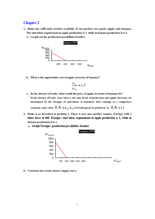
Chapter 21.Home has 1200 units of labor available. It can produce two goods, apples and bananas. The unit labor requirement in apple production is 3, while in banana production it is 2. a .Graph out the production possibilities frontier:b .What is the opportunity cost of apples in terms of bananas?5.1=LbLa a a c .In the absence of trade, what would the price of apples in terms of bananas be?In the absence of trade, since labor is the only factor of production and supply decisions aredetermined by the attempts of individuals to maximize their earnings in a competitive economy, only when Lb La b a /a a /P P =will both goods be produced. So 1.5 /P P b a =2.Home is as described in problem 1. There is now also another country, Foreign, with alabor force of 800. Foreign’s unit labor requirement in apple production is 5, while in banana production it is 1.a .Graph Foreign’s production possibilities frontier:b .3.Now suppose world relative demand takes the following form: Demand for apples/demandfor bananas = price of bananas/price of apples.a .Graph the relative demand curve along with the relative supply curve:a b b a /P P /D D =∵When the market achieves its equilibrium, we have 1b a )(D D −**=++=ba b b a a P P Q Q Q Q ∴RD is a hyperbola xy 1=b .What is the equilibrium relative price of apples?The equilibrium relative price of apples is determined by the intersection of the RD and RScurves.RD: yx 1= RS: 5]5,5.1[5.1],5.0(5.0)5.0,0[=∈=⎪⎩⎪⎨⎧+∞∈=∈y y y x x x ∴25.0==y x∴2/=b P a P e ec .Describe the pattern of trade.∵b a b e a e b a P P P P P P ///>>**∴In this two-country world, Home will specialize in the apple production, export applesand import bananas. Foreign will specialize in the banana production, export bananas and import apples.d .Show that both Home and Foreign gain from trade.International trade allows Home and Foreign to consume anywhere within the coloredlines, which lie outside the countries’ production possibility frontiers. And the indirect method, specializing in producing only one production then trade with other country, is a more efficient method than direct production. In the absence of trade, Home could gain three bananas by foregoing two apples, and Foreign could gain by one foregoing five bananas. Trade allows each country to trade two bananas for one apple. Home could then gain four bananas by foregoing two apples while Foreign could gain one apple by foregoing only two bananas. So both Home and Foreign gain from trade.4.Suppose that instead of 1200 workers, Home had 2400. Find the equilibrium relative price. What can you say about the efficiency of world production and the division of the gains from trade between Home and Foreign in this case? RD: yx 1= RS: 5]5,5.1[5.1],1(1)1,0[=∈=⎪⎩⎪⎨⎧+∞∈=∈y y y x x x ∴5.132==y x∴5.1/=b P a P e eIn this case, Foreign will specialize in the banana production, export bananas and import apples. But Home will produce bananas and apples at the same time. And the opportunity cost of bananas in terms of apples for Home remains the same. So Home neither gains nor loses but Foreign gains from trade.5.Suppose that Home has 2400 workers, but they are only half as production in both industries as we have been assuming, Construct the world relative supply curve and determine the equilibrium relative price. How do the gains from trade compare with those in the case described in problem 4?In this case, the labor is doubled while the productivity of labor is halved, so the "effective labor"remains the same. So the answer is similar to that in 3. And both Home and Foreign can gain from trade. But Foreign gains lesser compare with that in the case 4.6.”Korean workers earn only $2.50 an hour; if we allow Korea to export as m uch as it likes to the United States, our workers will be forced down to the same level. You can’t import a $5 shirt without importing the $2.50 wage that goes with it.” Discuss.In fact, relative wage rate is determined by comparative productivity and the relative demand for goods. Korea’s low wage reflects the fact that Korea is less productive than the United States in most industries. Actually, trade with a less productive, low wage country can raise the welfare and standard of living of countries with high productivity, such as United States. Sothis pauper labor argument is wrong.7.Japanese labor productivity is roughly the same as that of the United States in the manufacturing sector (higher in some industries, lower in others), while the United States, is still considerably more productive in the service sector. But most services are non-traded. Some analysts have argued that this poses a problem for the United States, because our comparative advantage lies in things we cannot sell on world markets. What is wrong with this argument?The competitive advantage of any industry depends on both the relative productivities of the industries and the relative wages across industries. So there are four aspects should be taken into account before we reach conclusion: both the industries and service sectors of Japan and U.S., not just the two service sectors. So this statement does not bade on the reasonable logic. 8.Anyone who has visited Japan knows it is an incredibly expensive place; although Japanese workers earn about the same as their U.S. counterparts, the purchasing power of their incomes is about one-third less. Extend your discussing from question 7 to explain this observation. (Hint: Think about wages and the implied prices of non-trade goods.) The relative higher purchasing power of U.S. is sustained and maintained by its considerably higher productivity in services. Because most of those services are non-traded, Japanese could not benefit from those lower service costs. And U.S. does not have to face a lower international price of services. So the purchasing power of Japanese is just one-third of their U.S. counterparts.9.How does the fact that many goods are non-traded affect the extent of possible gains from trade?Actually the gains from trade depended on the proportion of non-traded goods. The gains will increase as the proportion of non-traded goods decrease.10.We have focused on the case of trade involving only two countries. Suppose that there are many countries capable of producing two goods, and that each country has only one factor of production, labor. What could we say about the pattern of production and in this case? (Hint: Try constructing the world relative supply curve.)Any countries to the left of the intersection of the relative demand and relative supply curves export the good in which they have a comparative advantage relative to any country to the right of the intersection. If the intersection occurs in a horizontal portion then the country with that price ratio produces both goods.。
《国际经济学》克鲁格曼(第六版)习题答案imsect3
OVERVIEW OF SECTION III: EXCHANGE RATES AND OPEN ECONOMY MACROECONOMICSSection III of the textbook is comprised of six chapters:Chapter 12 National Income Accounting and the Balance of PaymentsChapter 13 Exchange Rates and the Foreign Exchange Market: An Asset Approach Chapter 14 Money, Interest Rates, and Exchange RatesChapter 15 Price Levels and the Exchange Rate in the Long RunChapter 16 Output and the Exchange Rate in the Short RunChapter 17 Fixed Exchange Rates and Foreign Exchange InterventionSECTION III OVERVIEWThe presentation of international finance theory proceeds by building up an integrated model of exchange rate and output determination. Successive chapters in Part III construct this model step by step so students acquire a firm understanding of each component as well as the manner in which these components fit together. The resulting model presents a single unifying framework admitting the entire range of exchange rate regimes from pure float to managed float to fixed rates. The model may be used to analyze both comparative static and dynamic time path results arising from temporary or permanent policy or exogenous shocks in an open economy.The primacy given to asset markets in the model is reflected in the discussion of national income and balance of payments accounting in the first chapter of this section. Chapter 12 begins with a discussion of the focus of international finance. The discussion then proceeds to national income accounting in an open economy. The chapter points out, in the discussion on the balance of payments account, that current account transactions must be financed by financial account flows from either central bank or noncentral bank transactions. A case study uses national income accounting identities to consider the link between government budget deficits and the current account.Observed behavior of the exchange rate favors modeling it as an asset price rather than as a goods price. Thus, the core relationship for short-run exchange-rate determination in the model developed in Part III is uncovered interest parity. Chapter 13 presents a model inwhich the exchange rate adjusts to equate expected returns on interest-bearing assets denominated in different currencies given expectations about exchange rates, and the domestic and foreign interest rate. This first building block of the model lays the foundation for subsequent chapters that explore the determination of domestic interest rates and output, the basis for expectations of future exchange rates and richer specifications of the foreign-exchange market that include risk. An appendix to this chapter explains the determination of forward exchange rates.Chapter 14 introduces the domestic money market, linking monetary factors to short-run exchange-rate determination through the domestic interest rate. The chapter begins with a discussion of the determination of the domestic interest rate. Interest parity links the domestic interest rate to the exchange rate, a relationship captured in a two-quadrant diagram. Comparative statics employing this diagram demonstrate the effects of monetary expansion and contraction on the exchange rate in the short run. Dynamic considerations are introduced through an appeal to the long run neutrality of money that identifies a long-run steady-state value toward which the exchange rate evolves. The dynamic time path of the model exhibits overshooting of the exchange-rate in response to monetary changes.Chapter 15 develops a model of the long run exchange rate. The long-run exchange rate plays a role in a complete short-run macroeconomic model since one variable in that model is the expected future exchange rate. The chapter begins with a discussion of the law of one price and purchasing power parity. A model of the exchange rate in the long-run based upon purchasing power parity is developed. A review of the empirical evidence, however, casts doubt on this model. The chapter then goes on to develop a general model of exchange rates in the long run in which the neutrality of monetary shocks emerges as a special case. In contrast, shocks to the output market or changes in fiscal policy alter the long run real exchange rate. This chapter also discusses the real interest parity relationship that links the real interest rate differential to the expected change in the real exchange rate. An appendix examines the relationship of the interest rate and exchange rate under a flexible-price monetary approach.Chapter 16 presents a macroeconomic model of output and exchange-rate determination in the short run. The chapter introduces aggregate demand in a setting of short-run price stickiness to construct a model of the goods market. The exchange-rate analysis presented in previous chapters provides a model of the asset market. The resulting model is, in spirit, very close to the classic Mundell-Fleming model. This model is used to examine the effects of avariety of policies. The analysis allows a distinction to be drawn between permanent and temporary policy shifts through the pedagogic device that permanent policy shifts alter long-run expectations while temporary policy shifts do not. This distinction highlights the importance of exchange-rate expectations on macroeconomic outcomes. A case study of U.S. fiscal and monetary policy between 1979 and 1983 utilizes the model to explain notable historical events. The chapter concludes with a discussion of the links between exchange rate and import price movements which focuses on the J-curve and exchange-rate pass-through. An appendix to the chapter compares the IS-LM model to the model developed in this chapter. A second appendix considers intertemporal trade and consumption demand. A third appendix discusses the Marshall-Lerner condition and estimates of trade elasticities.The final chapter of this section discusses intervention by the central bank and the relationship of this policy to the money supply. This analysis is blended with the previous chapter's short-run macroeconomic model to analyze policy under fixed rates. The balance sheet of the central bank is used to keep track of the effects of foreign exchange intervention on the money supply. The model developed in previous chapters is extended by relaxing the interest parity condition and allowing exchange-rate risk to influence agents' decisions. This allows a discussion of sterilized intervention. Another topic discussed in this chapter is capital flight and balance of payments crises with an introduction to different models of how a balance of payments or currency crisis can occur. The analysis also is extended to a two-country framework to discuss alternative systems for fixing the exchange-rate as a prelude to Part IV. An appendix to Chapter 17 develops a model of the foreign-exchange market in which risk factors make domestic-currency and foreign-currency assets imperfect substitutes.A second appendix explores the monetary approach to the balance of payments. The third appendix discusses the timing of a balance of payments crisis.。
克鲁格曼国际经济学答案(英文)
Overview of Section IInternational Trade TheorySection I of the text is comprised of six chapters: Chapter 2 Labor Productivity and Comparative Advantage: The Ricardian Model Chapter 3 Specific Factors and Income Distribution Chapter 4 Resources and Trade: The Heckscher-Ohlin Model Chapter 5 The Standard Trade Model Chapter 6 Economies of Scale, Imperfect Competition, and International Trade Chapter 7 International Factor Movements T Section I Overview Section I of the text presents the theory of international trade. The intent of this section is to explore the motives for and implications of patterns of trade between countries. The presentation proceeds by introducing successively more general models of trade, where the generality is provided by increasing the number of factors used in production, by increasing the mobility of factors of production across sectors of the economy, by introducing more general technologies applied to production, and by examining different types of market structure. Throughout Section I, policy concerns and current issues are used to emphasize the relevance of the theory of international trade for interpreting and understanding our economy. Chapter 2 gives a brief overview of world trade. In particular, it discusses what we know about the quantities and pattern of world trade today. The chapter uses the empirical relationship known as the gravity model as a framework to describe trade. This framework describes trade as a function of the size of the economies involved and their distance. It can then be used to see where countries are trading more or less than expected. The chapter also notes the growth in world trade over the previous decades and uses the previous era of globalization (pre-WWI) as context for today’s experience. Chapter 3 introduces you to international trade theory through a framework known as the Ricardian model of trade. This model addresses the issue of why two countries would want to trade with each other. This model shows how mutually-beneficial trade arises when there are two countries, each with one factor of production which can be applied toward producing each of two goods. Key concepts are introduced, such as the production possibilities frontier, comparative advantage versus absolute advantage, gains from trade, relative prices, and relative wages across countries. 4 Krugman/Obstfeld • International Economics: Theory and Policy, Seventh Edition Chapter 4 introduces what is known as the classic Heckscher-Ohlin model of international trade. Using this framework, you can work through the effects of trade on wages, prices and output. Many important and intuitive results are derived in this chapter including: the Rybczynski Theorem, the Stolper-Samuelson Theorem, and the Factor Price Equalization Theorem. Implications of the Heckscher-Ohlin model for the pattern of trade among countries are discussed, as are the failures of empirical evidence to confirm the predictions of the theory. The chapter also introduces questions of political economy in trade. One important reason for this addition to the model is to consider the effects of trade on income distribution. This approach shows that while nations generally gain from international trade, it is quite possible that specific groups within these nations could be harmed by this trade. This discussion, and related questions about protectionism versus globalization, becomes broader and even more interesting as you work through the models and different assumptions of subsequent chapters. Chapter 5 presents a general model of international trade which admits the models of the previous chapters as special cases. This “standard trade model” is depicted graphically by a general equilibrium trade model as applied to a small open economy. Relative demand and relative supply curves are used to analyze a variety of policy issues, such as the effects of economic growth, the transfer problem, and the effects of trade tariffs and production subsidies. The appendix to the chapter develops offer curve analysis. While an extremely useful tool, the standard model of trade fails to account for some important aspects of international trade. Specifically, while the factor proportions Heckscher-Ohlin theories explain some trade flows between countries, recent research in international economics has placed an increasing emphasis on economies of scale in production and imperfect competition among firms. Chapter 6 presents models of international trade that reflect these developments. The chapter begins by reviewing the concept of monopolistic competition among firms, and then showing the gains from trade which arise in such imperfectly competitive markets. Next, internal and external economies of scale in production and comparative advantage are discussed. The chapter continues with a discussion of the importance of intra-industry trade, dumping, and external economies of production. The subject matter of this chapter is important since it shows how gains from trade arise in ways that are not suggested by the standard, more traditional models of international trade. The subject matter also is enlightening given the increased emphasis on intra-industry trade in industrialized countries. Chapter 7 focuses on international factor mobility. This departs from previous chapters which assumed that the factors of production available for production within a country could not leave a country’s borders. Reasons for and the effects of international factor mobility are discussed in the context of a one-factor (labor) production and trade model. The analysis of the international mobility of labor motivates a further discussion of international mobility of capital. The international mobility of capital takes the form of international borrowing and lending. This facilitates the discussion of inter-temporal production choices and foreign direct investment behavior. 。
克鲁格曼《国际经济学》第八版课后答案(英文)-Ch06
克鲁格曼《国际经济学》第八版课后答案(英文)-Ch06Chapter 6Economies of Scale, Imperfect Competition, and International TradeChapter OrganizationEconomies of Scale and International Trade: An OverviewEconomies of Scale and Market StructureThe Theory of Imperfect CompetitionMonopoly: A Brief ReviewMonopolistic CompetitionLimitations of the Monopolistic Competition ModelMonopolistic Competition and TradeThe Effects of Increased Market SizeGains from an Integrated Market: A Numerical ExampleEconomies of Scale and Comparative AdvantageThe Significance of Intraindustry TradeWhy Intraindustry Trade MattersCase Study: Intraindustry Trade in Action: The North American Auto Pact DumpingThe Economics of DumpingCase Study: Anti-Dumping as ProtectionReciprocal DumpingThe Theory of External EconomiesSpecialized SuppliersLabor Market PoolingKnowledge SpilloversExternal Economies and Increasing Returns22 Krugman/Obstfeld ?International Economics: Theory and Policy, Eighth EditionExternal Economies and International TradeExternal Economies and the Pattern of TradeTrade and Welfare with External EconomiesBox: Tinseltown EconomicsDynamic Increasing ReturnsEconomic Geography and Interregional TradeSummaryAppendix: Determining Marginal RevenueChapter OverviewIn previous chapters, trade between nations was motivated by their differences in factor productivity or relative factor endowments. The type of trade which occurred, for example of food for manufactures, is based on comparative advantage and is called interindustry trade. This chapter introduces trade based on economies of scale in production. Such trade in similar productions is called intraindustry trade, and describes, for example, the trading of one type of manufactured good for another type of manufactured good. It is shown that trade can occur when there are no technological or endowment differences, but when there are economies of scale or increasing returns in production.Economies of scale can either take the form of (1) external economies, whereby the cost per unit depends on the size of the industry but not necessarily on the size of the firm; or as (2) internal economies, whereby the production cost per unit of output depends on the size of the individual firm but not necessarily on the size of the industry. Internal economies of scale give rise to imperfectly competitive markets, unlike the perfectly competitive market structures that were assumed to exist in earlier chapters. This motivatesthe review of models of imperfect competition, including monopoly and monopolistic competition. The instructor should spend some time making certain that students understand the equilibrium concepts of these models since they are important for the justification of intraindustry trade.In markets described by monopolistic competition, there are a number of firms in an industry, each of which produces a differentiated product. Demand for its good depends on the number of other similar products available and their prices. This type of model is useful for illustrating that trade improves the trade-off between scale and variety available to a country. In an industry described by monopolistic competition, a larger market—such as that which arises through international trade—lowers average price (by increasing production and lowering average costs) and makes available for consumption a greater range of goods. While an integrated market also supports the existence of a larger number of firms in an industry, the model presented in the text does not make predictions about where these industries will be located.It is also interesting to compare the distributional effects of trade when motivated by comparative advantage with those when trade is motivated by increasing returns to scale in production. When countries are similar in their factor endowments, and when scale economies and product differentiation are important, the income distributional effects of trade will be small. You should make clear to the students the sharp contrast between the predictions of the models of monopolistic competition and the specific factors and Heckscher-Ohlin theories of international trade. Without clarification, some students may find the contrasting predictionsof these models confusing.Another important issue related to imperfectly competitive markets is the practice of price discrimination, namely charging different customers different prices. One particularly controversial form of price discrimination is dumping, whereby a firm charges lower prices for exported goods than for goods sold domestically. This can occur only when domestic and foreign markets are segmented. The economicsChapter 6 Economies of Scale, Imperfect Competition, and International Trade 23 of dumping are illustrated in the text using the example of an industry which contains a single monopolistic firm selling in the domestic and foreign market. Reverse dumping can also occur, whereby a producer sells a product at lower prices in the domestic market than in the foreign market. While there is no good economic justification for the view that dumping is harmful, it is often viewed as an unfair trade practice.The other type of economies of scale, external economies, has very different economic implicationsthan internal economies. Since external economies of scale occur at the industry level rather than the firm level, it is possible for there to be many small competitors in an industry, in contrast to the structure which develops under internal economies of scale. Under external economies, trade may not be beneficial to all countries and there may be some justification for protectionism. Dynamic scale economies, which arise when unit production costs fall with cumulative production over time, rather than with current levels of production, also provide a potential justification for protectionism. External economies of scale can also be important for explaining interregional trade (trade within a country). While some industries need to belocated near a particular factor (e.g., a natural resource), for others, the factors (e.g., skilled labor) are fairly mobile. Historical accidents may help explain the patterns then. This study of the patterns of economic interactions across space—either within or across countries—is known as economic geography.Answers to Textbook Problems1. Cases a and d reflect external economies of scale since concentration of the production of an industryin a few locations reduces the industry’s costs even when the scale of operation of individual firms remains small. External economies need not lead to imperfect competition. The benefits of geographical concentration may include a greater variety of specialized services to support industry operations and larger labor markets or thicker input markets. Cases b and c reflect internal economies of scale and occur at the level of the individual firm. The larger the output of a product by a particular firm, the lower its average costs. This leads to imperfect competition as in petrochemicals, aircraft, and autos.2. The profit maximizing output level of a monopolist occurs where marginal revenue equals marginalcost. Unlike the case of perfectly competitive markets, under monopoly marginal revenue is not equal to price. Marginal revenue is always less than price under imperfectly competitive markets because to sell an extra unit of output, the firm must lower the price of all units, not just the marginal one.3. By concentrating the production of each good with economies of scale in one country rather thanspreading the production over several countries, the world economy will use the same amount of labor to produce more output. In the monopolistic competition model, such aconcentration of labor benefits the host country, which can also capture some monopoly rents, while it may hurt the rest of the world which could then face higher prices on its consumption goods. In the external economies case, such monopolistic pricing behavior is less likely since imperfectly competitive markets are less likely.4. Although this problem is a bit tricky and the numbers don’t work out nicely, a solution does exist.The first step in finding the solution is to determine the equilibrium number of firms in the industry.The equilibrium number of firms is that number, n, at which price equals average cost. We know that AC= F/X+c, where F represents fixed costs of production, X represents the level of sales by each firm, and c represents marginal costs. We also know that P= c+ (1/bn), where P and b represent price and the demand parameter. Also, if all firms follow the same pricing rule, then X= S/n where S equals total industry sales. So, set price equal to average cost, cancel out the c’s and replace X by S/n.Rearranging what is left yields the formula n2= S/Fb. Substitute in S= 900,000 + 1,600,000 +3,750,000 = 6,250,000, F= 750,000,000 and b= 1/30,000. The numerical answer is that n= 15.8 firms.However, since you will never see 0.8 firms, there will be 15 firms that enter the market, not 16 firms since the last firm knows that it can not make positive profits. The rest of the solution is straight-forward. Using X= S/n, output per firm is 41,666 units. Using the price equation, and the fact that c= 5,000, yields an equilibrium price of $7,000.24 Krugman/Obstfeld ?International Economics: Theory andPolicy, Eighth Edition5. a. 17,000 + 150/n= 5,000,000,000n/S+ 17,000. With S US= 300 million, the number of automakersequals three. With S E= 533 million, the number of automakers equals four.b. P US= 17,000 + 150/3, P US= $17,050. P E= 17,000 + 150/4, P US= $17,037.50.c. 17,000 + 150/n= 5,000,000,000n/S+ 17,000. With S US+E= 833 million, the number of totalautomakers now equals five. This helps to explain some of the consolidation that has happenedin the industry since trade has become more free in recent decades, e.g., Ford acquiring Jaguar,Daimler-Benz acquiring Chrysler, etc.d. Prices fall in the United States as well as Europe to $17,030. Also, variety increases in bothmarkets: in the United States, consumers were able to choose between three brands before freetrade; now they can choose between five. In Europe, consumers were able to choose betweenfour brands before free trade; now they can also choose between five brands.6. This is an open-ended question. Looking at the answer to Question 11 can provide some hints. Twoother examples would be: Biotechnology and Aircraft design. Biotechnology is an industry in which innovation fuels new products, but it is also one where learning how to successfully take an idea and create a profitable product is a skill set that may require some practice. Aircraft design requires both innovations to create new planes that are safer and or more cost efficient, butit is also an industry where new planes are often subtle alterations of previous models and where detailed experience with one model may be a huge help in creating a new one.7. a. The relatively few locations for production suggest external economies of scale in production.If these operations are large, there may also be large internal economies of scale in production.b. Since economies of scale are significant in airplane production, it tends to be done by a smallnumber of (imperfectly competitive) firms at a limited number of locations. One such locationis Seattle, where Boeing produces airplanes.c. Since external economies of scale are significant in semiconductor production, semiconductorindustries tend to be concentrated in certain geographic locations. If, for some historical reason, a semiconductor is established in a specific location, the export of semiconductors by that countryis due to economies of scale and not comparative advantage.d. “True” scotch whiskey can only come from Scotland. The production of scotch whiskey requiresa technique known to skilled distillers who are concentrated in the region. Also, soil and climacticconditions are favorable for grains used in local scotch production. This reflects comparativeadvantage.e. France has a particular blend of climactic conditions and land that is difficult to reproduceelsewhere. This generates a comparative advantage in wine production.8. The Japanese producers are price discriminating across United States and Japanese markets, so thatthe goods sold in the United States are much cheaper than those sold in Japan. It may be profitable for other Japanese to purchase these goods in the United States, incur any tariffs and transportation costs, and resell the goods in Japan. Clearly, the price differential across markets must be non-trivial for this to be profitable.Chapter 6 Economies of Scale, Imperfect Competition, and International Trade 25 9. a. Suppose two countries that can produce a good are subject to forward-falling supply curves and are identical countries with identical curves. If one country starts out as a producer of a good,i.e., it has a head start even as a matter of historical accident, then all production will occur in thatparticular country and it will export to the rest of the world.b. Consumers in both countries will pay a lower price for this good when external economies aremaximized through trade and all production is located in a single market. In the present example, no single country has a natural cost advantage or is worse off than it would be under autarky. 10. External economies are important for firms as technology changes rapidly and as the “cutting edge”moves quickly with frequent innovations. As this process slows, manufacturing becomes moreroutine and there is less advantage conferred by external economies. Instead, firms look for low cost production locations. Since external economies are no longer important, firms find little advantage in being clustered, and it is likely that locations other than the high-wage original locations are chosen.11. a. i. Very likely due to the need to have a common pool of labor with such skills.ii. Somewhat likely due to the need for continual innovation and learning.b. i. Unlikely since it is difficult to see how the costs of a single firm would fall if other firms arepresent in the asphalt industry.ii. Unlikely because they are industries in which technology is more stable than in other industries such as software services or cancer research.c. i. Highly likely because having a great number of support firms and an available pool of skilledlabor in filmmaking are critical to film production.ii. Highly likely because film making is an industry in which learning is important.d. i. Somewhat likely in that it may be advantageous to have other researchers nearby.ii. Highly likely because such research builds on itself through a learning-by-doing process.e. i. Unlikely because it is difficult to see how the existence of another timber firm with lowercosts to another timber firm.ii. Unlikely due to the relatively stable technology involved in timber harvesting.。
《国际经济学》克鲁格曼(第六版)习题答案imsect2
OVERVIEW OF SECTION II: INTERNATIONAL TRADE POLICYSection II of the text is comprised of four chapters:Chapter 8 The Instruments of Trade PolicyChapter 9 The Political Economy of Trade PolicyChapter 10 Trade Policy in Developing CountriesChapter 11 Strategic Trade Policies in Advanced CountriesSECTION II OVERVIEWTrade policy issues figure prominently in current political debates and public policy discussions. The first two chapters of this section of the text are concerned with the instruments of trade policy and the arguments for free trade and managed trade. The second two chapters consider these concepts in the context of specific sets of countries that face common problems. Throughout, the use of case studies provides the student with real world examples that clearly illustrate the theoretical arguments.Chapter 8 discusses various instruments of trade policy including tariffs, quotas, voluntary export restraints, and local content requirements. The effects of these policies on prices and trade volumes are determined in the context of a partial equilibrium framework. The chapter reviews the analytical tools of consumer and producer surplus, and uses these tools to consider the welfare effects of various protectionist measures. The specific incidents of trade restrictions presented as case studies include import quotas on sugar entering United States markets, voluntary export restraints on Japanese autos, and oil import quotas.Chapter 9 presents the set of ideas known as the political economy of trade theory. These ideas enable you to understand why certain trade restrictions exist, despite the force of general economic arguments which suggest that they reduce aggregate welfare. Possible motivations for trade restrictions are identified as those which increase national welfare, such as the optimum tariff, and those which foster either income redistribution or the preservation of status quo. While sometimes politically popular, these motivations for trade restrictions ignore the possibility of retaliation and usually fail tests based upon basic welfare analysis. Trade agreements of the 1990s are discussed, including the Uruguay Round, and distinctionsare made between Free Trade Areas and Customs Unions as well as between trade creation and trade diversion.Chapter 10 considers the possible uses of trade policies to promote the growth of developing economies. The chapter reviews the relative successes of different development strategies. It examines arguments for and the results of import-substituting industrialization. The phenomenon of economic dualism, referring to the coexistence of capital intensive industrial sectors and low-wage traditional sectors, and of uneven development are considered. The chapter concludes with a discussion of export led growth and the experience of the high performing Asian economies.Chapter 11 considers recent controversies in trade policy. The first part of the chapter considers the notion of strategic trade policy, which first arose in the 1990s. Strategic trade policy refers to the use of trade (and other) tools for channeling resources to sectors targeted for growth by industrial country governments. The chapter presents some commonly voiced arguments for intervention in particular sectors of the economy, and then shows how these arguments are critically flawed. The second part of the chapter introduces more sophisticated arguments for strategic trade policy. The most persuasive of these is the existence of some form of market failure. The second part of the chapter considers the impact of rising trade on workers in developing countries, and more broadly, the debate over globalization. This debate has been argued in academia and policy circles, but also on the streets of Seattle, Genoa, and other cities hosting global economic summits.。
国际经济学克鲁格曼教材答案完整版

国际经济学克鲁格曼教材答案HUA system office room 【HUA16H-TTMS2A-HUAS8Q8-HUAH1688】Problems and Answers to Chapter 2Q1: Canada and Australia are (mainly) English-speaking countries with populations that are not too different in size (Canada’s is 60 percent larger). But Canadian trade is twice as large, relative to GDP, as Australia’s. Why should this be the case加拿大和澳大利亚都是英语国家,两国的人口规模也相当(加拿大多60%),但是相对各自的GDP而言,加拿大的贸易额是澳大利亚的两倍,为什么如此?A1:According to Gravity Model, GDP is not the only factor to explain the volume oftrade between two countries, because distance is also an important factor. Consideringthe distance, the transportation cost of Australia is relatively higher than that ofCanada, so the attractiveness of trade is reduced. However, Canada is close to theUSA which is a large economy while Australia is not close to any large economy,making Canada more open while Australia is more autarky.GDP 不是解释两国贸易量的唯一重要因素,距离也是至关重要的因素之一。
- 1、下载文档前请自行甄别文档内容的完整性,平台不提供额外的编辑、内容补充、找答案等附加服务。
- 2、"仅部分预览"的文档,不可在线预览部分如存在完整性等问题,可反馈申请退款(可完整预览的文档不适用该条件!)。
- 3、如文档侵犯您的权益,请联系客服反馈,我们会尽快为您处理(人工客服工作时间:9:00-18:30)。
3. a. The relative demand curve includes the points (1/5, 5), (1/2, 2), (1,1), (2,1/2).
b. The equilibrium relative price of apples is found at the intersection of the relative demand and relative supply curves. This is the point (1/2, 2), where the relative demand curve intersects the vertical section of the relative supply curve. Thus the equilibrium relative price is 2.
2. a. The production possibility curve is linear, with the intercept on the apple axis equal to 160 (800/5) and the intercept on the banana axis equal to 800 (800/1).
b. The opportunity cost of apples in terms of bananas is 3/2. It takes three units of labor to harvest an apple but only two units of labor to harvest a banana. If one foregoes harvesting an apple, this frees up three units of labor. These 3 units of labor could then be used to harvest bananas.
c. Labor mobility ensures a common wage in each sector and competition ensures the price of goods equals their cost of production. Thus, the relative price equals the relative costs, which equals the wage times the unit labor requirement for apples divided by the wage times the unit labor requirement for bananas. Since wages are equal across sectors, the price ratio equals the ratio of the unit labor requirement, which is 3 apples per 2 bananas.
b. The world relative supply curve is constructed by determining the supply of apples relative to the supply of bananas at each relative price. The lowest relative price at which apples are harvested is 3 apples per 2 bananas. The relative supply curve is flat at this price. The maximum number of apples supplied at the price of 3/2 is 400 supplied by Home while, at this price, Foreign harvests 800 bananas and no apples, giving a maximum relative supply at this price of 1/2. This relative supply holds for any price between 3/2 and 5. At the price of 5, both countries would harvest apples. The relative supply curve is again flat at 5. Thus, the relative supply curve is step shaped, flat at the price 3/2 from the relative supply of 0 to 1/2, vertical at the relative quantity 1/2 rising from 3/2 to 5, and then flat again from 1/2 to infinity.
克鲁格曼国际经济学课后答案英vity and Comparative Advantage: The Ricardian Model
Answers to Textbook Problems
1.a. The production possibility curve is a straight line that intercepts the apple axis at 400 (1200/3) and the banana axis at 600 (1200/2).