汽车侧向动力学
汽车二自由度动力学模型

汽车二自由度动力学模型
汽车二自由度动力学模型是一种用于描述汽车运动的简化模型。
它考虑了两个自由度,通常是车辆的纵向(前进方向)和侧向(横向)运动。
在这个模型中,车辆被视为一个质量集中的刚体,通过两个自由度来描述其运动状态。
这两个自由度通常是车辆的速度(纵向)和横摆角速度(侧向)。
汽车二自由度动力学模型的建立基于一些基本的物理原理,如牛顿第二定律、动量守恒定律和刚体动力学。
通过对这些原理的应用,可以得到描述车辆运动的微分方程。
这些方程通常包括车辆的加速度、驱动力或制动力、转向力矩以及车辆的惯性参数等。
通过求解这些微分方程,可以预测车辆在不同工况下的运动响应,例如加速、制动、转弯等。
汽车二自由度动力学模型在车辆动力学研究、驾驶模拟器、自动驾驶系统等领域有广泛应用。
它可以帮助工程师和研究人员了解车辆的基本运动特性,评估车辆的操控稳定性、行驶安全性等方面的性能。
然而,需要注意的是,二自由度模型是一种简化的模型,它忽略了许多实际情况中的复杂因素,如悬挂系统、轮胎特性、空气动力学等。
在实际应用中,可能需要使用更复杂的多自由度模型或考虑更多的因素来更准确地描述汽车的运动。
总的来说,汽车二自由度动力学模型提供了一个简单而有用的工具,用于初步研究和理解汽车的运动行为,但在具体应用中,需要根据实际需求进行适当的修正和扩展。
如果你对汽车动力学模型有更深入的问题或需要进一步的讨论,我将很愿意提供帮助。
第四章汽车转向操纵系统动力学
m0 h c b1 b0
式中 m0 mIz ;
h [mD Iz A];
c mB (AD B2 ) ;
(4 16)
b1 mLa K1;
b0 LK1K 2
回主目录
如果令 r ,则式(4-16)可写成
m0r hr cr b1 b0
(4 17)
这是一个强迫振动的二阶微分方程,可进一步改写为
K
此时
max ch 2L
回主目录
此最大值为轴距L相等的中性转向汽车横摆角
速转代度向轿增量车益增把的加特一时征半,车,即速此设K增时计大为,c6h特5称~征为1车0特0速k征m车/ hch速之。降间当低。不,足当
3. K<0 此时式(4-9)中的分母小于1,横摆角速度增益
比中性转向时大,随着车速的增加,曲线将
回主目录
在国外把这一比值称为静态储备系数S·M(Static
Margin), S M La La K 2 La (4 13)
L
K1 K 2 L
当中性转向作用点
C
与质心重合时,
n
La
L'a
S M 0 中性转向( a1 a2 )
当质心在中性转向作用点之前, La L'a
S M 0 不足转向( a1 a2 )
先将式(4-5)、(4-6)改写成下式 :
A BB DK1aK m1(Iz)
式中 A K1 K 2
B (La Ka1 Lb Ka2 )
D (La 2 K1 Lb 2 K 2 )
(4 14)
(4 15)
回主目录
由式(4-15)得
( I z
D
K1
)
B
代人式(4-14)中消去 ,最后可整理成的微分方程:
汽车理论:汽车侧向动力学

同济大学,汽车学院 左曙光教授教案
前轮角阶跃作用下的汽车稳态响应
汽车侧向动力学两自由度模型: ωr ⎧ & − k 1δ = m (υ + u ω r ) ⎪ ( k 1 + k 2 ) β + ( L1 k 1 − L 2 k 2 )
⎪ u ⎨ ⎪ ( L k − L k ) β + ( L2 k − L2 k ) ω r − L k δ = I ω &r 1 1 2 2 1 1 2 2 1 1 z ⎪ u ⎩
K =0
ωr ⎞ u ⎟ = δ ⎠S L
ωr =
u ωr ⎞ = ⎟ 横摆角速度增益: δ ⎠S L 汽车作与速度无关的圆周运动
u 横摆角速度: ωr = ⋅ δ L
u ⋅δ L u ωr = R
R=
δ
L
(与速度无关)
同济大学,汽车学院 左曙光教授教案
前轮角阶跃作用下的汽车稳态响应
ωr ⎞ u/L u/L = = ⎟ δ ⎠ S 1 + m ( L1 − L2 )u 2 1 + Ku 2 2
实验工况:车速 22.35m/s;侧向加速度 0.4g
同济大学,汽车学院 左曙光教授教案
前轮角阶跃作用下的汽车稳态响应
u/L ωr ⎞ u/L = ⎟ = δ ⎠ S 1 + m ( L1 − L2 )u 2 1 + Ku 2 2 L k2 k1
稳态横摆角速度 益或转向灵敏度
稳态响应的三种类型: 1、中性转向
同济大学,汽车学院 左曙光教授教案
汽车轮Байду номын сангаас的侧偏特性(复习)
当侧偏角不超过4~5度时,侧偏角和 侧偏力成线性关系,汽车正常行驶 驶时,侧向加速度不超过0.4g,侧 偏角不超过4~5度。
汽车理论:汽车侧向动力学

=
−(δ
−ξ)
=
β
+
L1ωr
u
−δ
α2
= υ − L2ωr
u
=
β
−
L2ωr
u
前轮和后轮侧偏力:
FY1 = k1α1
FY 2 = k2α 2
同济大学,汽车学院 左曙光教授教案
汽车线性两自由度模型
⎧ ⎨ ⎩
k 1α
L1k
1+
1α 1
k 2α
−L
2=m
2 k 2α 2
(u =
ω
I
r+
z ω& r
υ&
)
将
ωr δ
⎟⎞ ⎠S
=
u/L 1+ Ku2
δ = (1+ K ) ⋅u2 ⋅ L 保持半径不变 R
δ
K >0
K =0
K <0
现代轿车, 侧向加速度0.3g时,K ≈ 0.0024s2 m2 侧向加速度0.5g时,K ≈ 0.0026s2 m2
同济大学,汽车学院 左曙光教授教案
几个表征稳态响应的参数
1、前后轮侧偏角之差 (α1 −α2 )
uch =
−1 K
当 uch =
− 1 时 (临界车速 ), K
ωr δ
⎟⎞ ⎠K <0
=
∞
K ↑, uch ↓ 过多转向越大
u → uch时, 很小的δ 也会ωr (∞), 产生急转、 侧滑和翻车
同济大学,汽车学院 左曙光教授教案
前轮角阶跃作用下的汽车稳态响应
稳态响应的三种类型:不足转向、中性转向、过度转向
实验工况:车速 22.35m/s;侧向加速度 0.4g
三轴汽车前后轮转向时的侧向动力学控制
中 图分 类普 6 U4
文献标识鹂 ; A
A p ie M o e — l wi g Co t o o o r W h e te ig Ve i l da t d lFol r o n nrl fF u — e lS e r n h c e
维普资讯
第 2 1卷 第 1期
2 02年 0
1 月
ME HA c c NI A
擂 c 。 G HLY N。
Ju 22 V. N 1 aa 0 n】 0 or 1y 2
文 童 编 号 :0 88 2 ( 0 20 — 0 90 1 0 —7 8 2 0 ) 10 6 —3
O r n n e twh e sa d o t rdit r a c a y o e i t d r n .Th d l o] wig v ra l tu — ff o ta d r s e l n u e s u b n e v r v ra] e a ge mi e mo e— L n a ibe s r c f o
GUAN — ln QU u z e Z Xiq a g, Qi h n, HANG i n wu Ja — ( a h i io o g Un v r iy, h n h i2 0 3 ) Sh ng a a t n ie st S a g a 1 0 0 J
Ab t a t Th p i [se n o t o sr c : e o tma t e i gc n r lawso e rwh es f rt r e a l e il n c mplx t p c lp t r t id r l fr a e l o h e — x ev hc eo o e y ia a h ae sude h d n t e c r an v h ce mod lo l s d—o p c n r 1 a h e ti e il e fco e lo o t o .T h t e i g r s n e fv hil r m p o e h o g e se rn epo s s 0 e c ea ei r v d t r u h
04第四章 汽车转向系统动力学

4.3.2 驾驶员对转向盘的操纵作用与汽 车运动稳定性
现实中的k h 只能取兼顾二者的 适当值。 具体表现在,驾驶员在操纵汽车高速行使 时,既不是紧握乃至完全固定转向盘从而 使k h 很大,也不是完全从转向盘撒手而使 k h为0,而是以适当的力度轻轻握住转向 盘,从而获得合适的k h 。可以说,驾驶员 轻轻搭在转向盘上的 手、腕的作用是使汽 车运动更趋稳定。
(4-9)
(4-10)
式中:前轮转向角、前后轮各侧偏角以及各侧偏力 如图4-6a所示;
m,Iz——汽车质量、绕质心C的转动惯量;
lf、lr——质心C至前、后轴的距离。
又参照图4-6b,可以分别确定各车轮侧偏角为:
f 1 tan f 1
f 2 tan f 2
V l f r V d f r 2
lf d Ih 2k f ( r ) Th 2 dt V
(4-2)’’
当 时:
d 2 mV 2(k f kr ) m V (l f k f lr kr )r 2k f 0(4-30) dt V
dr 2(l f k f lr kr ) I Z dt
(4-19)
dr 2(l ek f l k ) 2(l f ek f lr kr ) I Z r 2l f ek f dt V
2 f 2 f r
比较式(4-19)、(4-20)与 (4-15)、(4-16)可知,前者实际上 相当于是用e kf 和a分别代替后者的kf 和 .
r
(4-61)
车速80km/h,1g=9.8m/s2 图4-18 与前轮转角成比例的后轮转向对汽车侧向加速度响应的影响
汽车高等动力学讲解
汽车高等动力学讲解-CAL-FENGHAI.-(YICAI)-Company One1侧偏力:汽车在行驶过程中,由于路面的侧向倾斜、侧向风、或者曲线行驶时的离心力等的作用,车轮中心沿Y轴方向将作用有侧向力F y,相应地在地面上产生地面侧向反作用力F Y,F Y即侧偏力。
侧偏现象:当车轮有侧向弹性时,即使F Y没有达到附着极限,车轮行驶方向也将偏离车轮平面cc,这就是轮胎的侧偏现象。
侧偏角:车轮与地面接触印迹的中心线与车轮平面错开一定距离,而且不再与车轮平面平行,车轮印迹中心线跟车轮平面的夹角即为侧偏角。
高宽比:以百分数表示的轮胎断面高H与轮胎断面宽B 之比 H/B×100% 叫高宽比.附着椭圆:它确定了在一定附着条件下切向力与侧偏力合力的极限值。
转向灵敏度:汽车等速行驶时,在前轮角阶跃输入下进入的稳态响应就是等速圆周行驶。
常用输出与输入的比值,如稳态的横摆角速度与前轮转角之比来评价稳态响应,这个比值称为稳态横摆角速度增益,也就是转向灵敏度。
(即稳态的横摆角速度与前轮转角之比)稳定性因数:稳定性因数单位为s2/m2,是表征汽车稳态响应的一个重要参数。
侧倾轴线:车厢相对于地面转动时的瞬时轴线称为车厢侧倾轴线。
侧倾中心:车厢侧倾轴线通过车厢在前,后轴处横断面上的瞬时转动中心,这两个瞬时中心称为侧倾中心。
悬架的侧倾角刚度:悬架的侧倾角刚度是指侧倾时(车轮保持在地面上),单位车厢转角下,悬架系统给车厢总的弹性恢复力偶矩。
转向盘力特性:转向盘力随汽车运动状况而变化的规律称为转向盘力特性。
切向反作用力控制的三种类型:总切向反作用力控制,前后轮间切向力分配比例的控制,内外侧车轮间切向力分配的控制。
侧翻阈值:汽车开始侧翻时所受的侧向加速度称为侧翻阈值。
汽车的平顺性:汽车的平顺性主要是保持汽车在行驶过程中产生的振动和冲击环境对乘员舒适性的影响在一定界限之内,主要根据乘员的主观感觉的舒适性来评价。
1.汽车的操纵稳定性:是指在驾驶者不感到过分紧张、疲劳的情况下,汽车能遵循驾驶者通过转向系统及转向车轮给定的方向行驶,且当遭遇外界干扰时,汽车能抵抗干扰而保持稳定行驶的能力。
汽车侧向速度计算公式
汽车侧向速度计算公式
汽车侧向速度的计算公式通常涉及到车辆的侧向位移和所经历的时间。
侧向速度(V_lateral)可以定义为车辆在单位时间内沿侧向方向(垂直于车辆前进方向)移动的距离。
公式如下:
V_lateral = ΔD_lateral / Δt
其中:
•ΔD_lateral 是车辆在侧向方向上的位移量,即车辆从一个点到另一个点在侧向方向上移动的距离。
•Δt 是所经历的时间,即测量位移所花费的时间段。
这个公式提供了一个基本的框架来计算侧向速度。
然而,在实际情况中,侧向速度的计算可能会更加复杂,因为它可能受到多种因素的影响,如车辆的转向角、轮胎的侧偏角、路面条件等。
这些因素可能需要通过更高级的物理模型或车辆动力学模型来考虑。
请注意,这个公式假设侧向位移和时间都是准确测量的,并且忽略了任何可能影响侧向速度的外部因素。
在实际应用中,可能需要使用更精确的测量设备和更复杂的模型来获得更准确的侧向速度估计。
侧滑动力学
侧滑动力学
侧滑动力学是指在车辆运动中,车辆在行驶过程中发生侧向运动的力学现象和相关的研究。
侧滑通常发生在车辆转弯或执行其他横向运动时,这时车辆的轮胎与行驶方向不一致,产生了侧向力,导致车辆出现横向的侧滑运动。
以下是侧滑动力学中一些重要的概念和因素:
1.侧滑角(Side Slip Angle):侧滑角是指车辆行驶方向与车辆速度方向之间的夹角。
当车辆转弯时,由于轮胎的滑移,车轮的方向与车辆速度方向产生差异,形成侧滑角。
2.侧向力(Lateral Force):侧向力是车辆在侧向运动中产生的力。
它是由轮胎与地面之间的相互作用引起的,通常与侧滑角成正比。
3.横摆稳定性:横摆稳定性描述了车辆在横向运动中的稳定性。
一个稳定的车辆在转弯过程中更容易保持方向稳定,而不容易出现过度的侧滑。
4.侧滑角的控制:车辆动力学控制系统通常包括侧滑角的控制。
通过使用车辆稳定性系统、防抱死制动系统(ABS)和电子稳定控制系统(ESC)等技术,可以减少侧滑并提高车辆的稳定性。
5.轮胎特性:轮胎是影响侧滑动力学的重要因素。
轮胎的抓地力、橡胶硬度、胎纹设计等因素都会影响车辆在侧向运动中的性能。
侧滑动力学的研究对于改善车辆的操控性能、提高驾驶安全性以及优化车辆稳定性具有重要意义。
在汽车工程领域,工程师通过模拟和测试来了解车辆的侧滑动力学特性,并设计相应的控制系统以提高车辆的性能和安全性。
汽车高等动力学分析解析
侧偏力:汽车在行驶过程中,由于路面的侧向倾斜、侧向风、或者曲线行驶时的离心力等的作用,车轮中心沿Y轴方向将作用有侧向力F y,相应地在地面上产生地面侧向反作用力F Y,F Y即侧偏力。
侧偏现象:当车轮有侧向弹性时,即使F Y没有达到附着极限,车轮行驶方向也将偏离车轮平面cc,这就是轮胎的侧偏现象。
侧偏角:车轮与地面接触印迹的中心线与车轮平面错开一定距离,而且不再与车轮平面平行,车轮印迹中心线跟车轮平面的夹角即为侧偏角。
高宽比:以百分数表示的轮胎断面高H与轮胎断面宽B 之比 H/B×100% 叫高宽比.附着椭圆:它确定了在一定附着条件下切向力与侧偏力合力的极限值。
转向灵敏度:汽车等速行驶时,在前轮角阶跃输入下进入的稳态响应就是等速圆周行驶。
常用输出与输入的比值,如稳态的横摆角速度与前轮转角之比来评价稳态响应,这个比值称为稳态横摆角速度增益,也就是转向灵敏度。
(即稳态的横摆角速度与前轮转角之比)稳定性因数:稳定性因数单位为s2/m2,是表征汽车稳态响应的一个重要参数。
侧倾轴线:车厢相对于地面转动时的瞬时轴线称为车厢侧倾轴线。
侧倾中心:车厢侧倾轴线通过车厢在前,后轴处横断面上的瞬时转动中心,这两个瞬时中心称为侧倾中心。
悬架的侧倾角刚度:悬架的侧倾角刚度是指侧倾时(车轮保持在地面上),单位车厢转角下,悬架系统给车厢总的弹性恢复力偶矩。
转向盘力特性:转向盘力随汽车运动状况而变化的规律称为转向盘力特性。
切向反作用力控制的三种类型:总切向反作用力控制,前后轮间切向力分配比例的控制,内外侧车轮间切向力分配的控制。
侧翻阈值:汽车开始侧翻时所受的侧向加速度称为侧翻阈值。
汽车的平顺性:汽车的平顺性主要是保持汽车在行驶过程中产生的振动和冲击环境对乘员舒适性的影响在一定界限之内,主要根据乘员的主观感觉的舒适性来评价。
1.汽车的操纵稳定性:是指在驾驶者不感到过分紧张、疲劳的情况下,汽车能遵循驾驶者通过转向系统及转向车轮给定的方向行驶,且当遭遇外界干扰时,汽车能抵抗干扰而保持稳定行驶的能力。
汽车侧向动力学

“高速汽车行驶的生命线”(汽车主动安全的主要内容)
同济大学,汽车学院 左曙光教授教案
汽车操纵稳定性的内容
• 操纵稳定性中,常把汽车作为一个控制系统,求汽车曲线行 驶的时域响应与频域响应。
路面条件 交通状况
汽车理论
汽车侧向动力学 (汽车的操纵稳定性)
2011年11月
同济大学,汽车学院 左曙光教授教案
汽车操纵稳定性的含义
定义:
在驾驶员不感觉过分紧张、疲劳的条件下,汽车能按照驾驶 员通过转向系及转向车轮给定的方向行驶,且当受到外界干扰
时,汽车能抵抗干扰而保持稳定行驶的能力。
1、操纵性:汽车能确切地按驾驶员通过方向盘给定的转向 指令行驶的能力。反映汽车实际行驶轨迹与驾驶员主观意图在 时间及空间上吻合程度。
r
S
u/L 1 Ku2
u L
对转向灵敏度公式取极值(求导为零):
uch
1 K
同济大学,汽车学院 左曙光教授教案
前轮角阶跃作用下的汽车稳态响应
稳态响应的三种类型:
稳态横摆角速度 增益或转向灵敏 度
3、过多转向
r
S
1
uL K u
2
在转向盘角一定时,若要增加车速并 维持转向半径不变,则原有的转向盘 角显得过大,需要减小转向盘转角。
r横摆角速度( yaw)
w垂直速度
p侧倾角速度(roll )
u前进速度
q俯仰角速度( pitch) 侧向速度
同济大学,汽车学院 左曙光教授教案
汽车操纵稳定性的内容及评价参量
基本内容
评价参量
转向盘角阶跃输入下的稳态响 稳态横摆角速度增益—转向灵敏度﹑前﹑后轮侧偏
汽车转向系统动力学(五.六)
- 汽车转向系统动力学
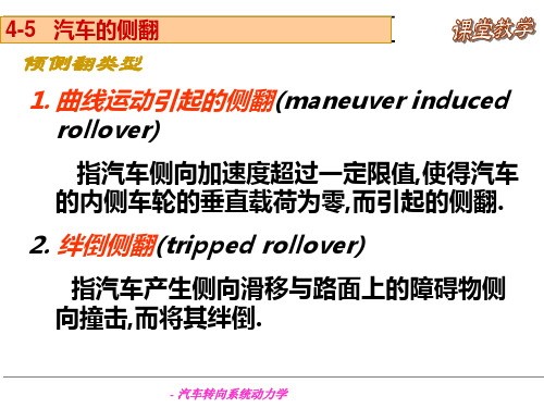
4-5 汽车的侧翻
刚性汽车的准静态侧翻
ay 1 F zi B g 2 m g hg
1 时,若要使 F zi 2 mg
当
ay 0
则有
ay g
v
2
g
高速公路拐弯处的坡道角就是根据此原理设计的.
- 汽车转向系统动力学
4-5 汽车的侧翻
- 汽车转向系统动力学
4-6 提高操纵稳定性的电子控制系统
各个车轮制动力控制的效果
施加小制动力时,可以利 用单个车轮进行控制。右 图是对每个车轮单独施加 500N制动力时转向半径随 时间变化的曲线。可以看 出,在后内轮施加制动力 的效果最好。
- 汽车转向系统动力学
4-6 提高操纵稳定性的电子控制系统
Fy1· x2· y2· a+F B-F b=0
Fx2减小不足转向量
- 汽车转向系统动力学
4-6 提高操纵稳定性的电子控制系统
直接横摆力矩控制(Direct Yaw Moment Control)
(改变内外侧车轮驱动力分配比例提高极限工况下弯道行驶能力)
a:一般行驶 b:有横摆力矩作用,加速行驶,Fy1减小
- 汽车转向系统动力学
D: driving force distribution B: braking force distribution R: roll stiffness distribution
汽车四轮转向四自由度动力学模型
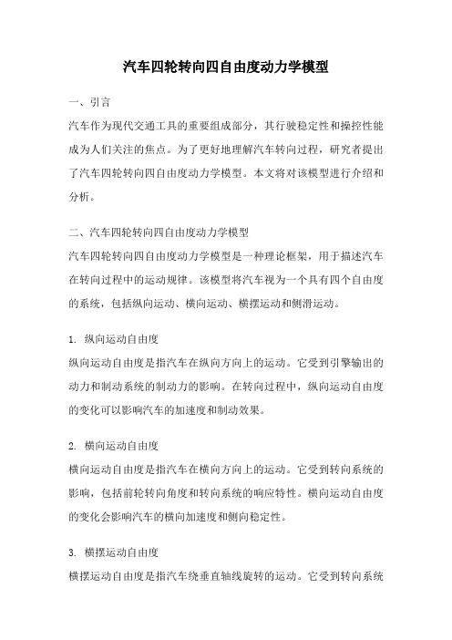
汽车四轮转向四自由度动力学模型一、引言汽车作为现代交通工具的重要组成部分,其行驶稳定性和操控性能成为人们关注的焦点。
为了更好地理解汽车转向过程,研究者提出了汽车四轮转向四自由度动力学模型。
本文将对该模型进行介绍和分析。
二、汽车四轮转向四自由度动力学模型汽车四轮转向四自由度动力学模型是一种理论框架,用于描述汽车在转向过程中的运动规律。
该模型将汽车视为一个具有四个自由度的系统,包括纵向运动、横向运动、横摆运动和侧滑运动。
1. 纵向运动自由度纵向运动自由度是指汽车在纵向方向上的运动。
它受到引擎输出的动力和制动系统的制动力的影响。
在转向过程中,纵向运动自由度的变化可以影响汽车的加速度和制动效果。
2. 横向运动自由度横向运动自由度是指汽车在横向方向上的运动。
它受到转向系统的影响,包括前轮转向角度和转向系统的响应特性。
横向运动自由度的变化会影响汽车的横向加速度和侧向稳定性。
3. 横摆运动自由度横摆运动自由度是指汽车绕垂直轴线旋转的运动。
它受到转向系统和车身结构的影响,包括转向系统的转向角速度和车身的转动惯量。
横摆运动自由度的变化会影响汽车的横摆角度和横摆稳定性。
4. 侧滑运动自由度侧滑运动自由度是指汽车的轮胎与地面之间的相对滑动。
它受到横向运动和横摆运动的影响,包括车轮滑动角度和侧向力的变化。
侧滑运动自由度的变化会影响汽车的侧向力和侧滑稳定性。
三、应用与研究进展汽车四轮转向四自由度动力学模型在汽车工程领域具有广泛的应用价值。
它可以用于汽车设计和操控性能评估,帮助工程师改进汽车的转向系统和悬挂系统,提高汽车的稳定性和操控性能。
研究者们在汽车四轮转向四自由度动力学模型的基础上进行了许多深入的研究。
他们通过理论模拟和实验验证,对汽车转向过程中的动力学特性进行了深入分析,为汽车操控性能的提升提供了重要的理论支持。
随着自动驾驶技术的发展,汽车四轮转向四自由度动力学模型也得到了进一步的应用。
研究者们通过建立更加精确的模型,优化汽车的自动驾驶算法,提高汽车的驾驶安全性和舒适性。
汽车动力学基础 第七章 汽车侧倾动力学

当汽车承受侧向力时,车身便相对地发生侧向倾斜,使法向力在左、右轮 间重新分配,影响着弹性轮胎的侧偏特性,还引起前轮定位参数发生变化以及 侧倾转向,从而影响汽车稳态及瞬间转向特性等。
过大的车身侧倾会使车辆发生绕其纵轴旋转90o以上的侧翻,造成严重的交 通事故。
车侧倾动力学主要内容包括侧倾中心、车轮侧倾外倾、侧倾转向、侧倾动 力学模型、汽车侧翻运动及抗侧倾性评价指标等。目前,汽车侧倾动力学在客 车、货车等高质心商用车研究和开发中受到更多重视。
ks
m
2
n
整个悬架的线刚度
Kl
2ks
m n
2
Δφr Δst
Δss
Cs Gs
m n
FZ
7.2.2 悬架的侧倾角刚度
悬架的侧倾角刚度:在单位车身侧倾转 角下(车轮保持在地面上),悬架系统
Kl
B 2
d
施加给车身总的弹性恢复力偶矩。
dT
K d
Kl
车身发生小侧倾角dφ时
dT
2
K
' l
B 2
d
B 2
7.1 侧倾几何学 7.1.1 侧倾中心
车身在前、后轴处横断面上的瞬时转动中心。
O24
Om
vd
E
F
D
G
vg
单横臂独立悬架侧倾中心
O23
O12
2
3
O13
1 4
O14
O34
四连杆机构的相对运动瞬心
7.1 侧倾几何学 7.1.1 侧倾中心 :车身在前、后轴处横断面上的瞬时转动中心。
vd
Ol
Om
vd
Ol
FYγl FYαl
汽车横向动力学模型推导过程
汽车横向动力学模型推导过程
汽车横向动力学模型是研究汽车在行驶过程中的侧向运动特性的数学模型。
它通过描述车辆的侧向运动方程,来分析车辆在转弯、横向加速等情况下的行驶性能。
下面将从车辆的侧向力、横向加速度和车辆的稳定性等方面,来介绍汽车横向动力学模型的推导过程。
一、车辆的侧向力
车辆在转弯或横向加速时,轮胎与地面之间会产生侧向力。
侧向力可以分为横向力和法向力两个分量。
横向力是垂直于车辆的运动方向的力,它使车辆产生侧向加速度;法向力是垂直于地面的力,它支撑着车辆的重力。
二、横向加速度
横向加速度是描述车辆在横向运动时的加速度大小,它与车辆的侧向力和车辆的质量有关。
根据牛顿第二定律,车辆的横向加速度等于车辆的侧向力除以车辆的质量。
三、车辆的稳定性
车辆的稳定性是指车辆在转弯或横向加速时保持平衡的能力。
车辆的稳定性与车辆的质心高度、轴距、重心位置等因素有关。
当车辆的质心高度较低、轴距较大、重心位置较低时,车辆的稳定性较好。
四、车辆的横向动力学模型
汽车横向动力学模型是基于上述车辆的侧向力、横向加速度和车辆
的稳定性等因素建立起来的数学模型。
它可以描述车辆在转弯或横向加速时的运动特性。
汽车横向动力学模型是通过分析车辆的侧向力、横向加速度和车辆的稳定性等因素,来推导出车辆在转弯或横向加速时的运动特性的数学模型。
这个模型可以帮助我们更好地理解车辆的横向运动特性,为汽车设计和操控提供参考。
基于观测器的汽车侧向动力学控制
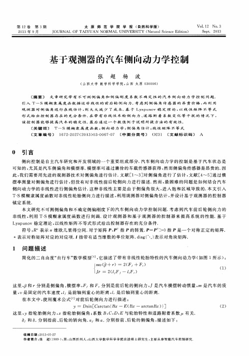
( 1 )
这里 , 和 r分 别是 侧偏 角 、 横 摆率 , F, 和F 分 别是前 后 轮 的侧 向力 , J是 汽车横 摆转 动惯 量 , m 是 汽 车 的质
量, 是 固定 的汽车速 度 , z , 是前 轴到 重心 的距 离 , l 是 后轴 到重 心 的距 离. 在本 文 中 , 使 用魔术 公 式l _ 7 对 前后 轮侧 向力 进行 描述 :
[ 关 键词 ] T — S模 糊 隶 属 度 函 数 ; 侧 向动 力学 ; 侧 偏 角估计 ; 线 性 矩 阵 不 等 式 ( 文章编 号] 1 6 7 2 — 2 0 2 7 ( 2 0 1 3 ) 0 3 — 0 0 6 7 — 0 7 [ 中图分类 号] o2 3 1 [ 文 献标识 码] A
T — S模糊 隶属 度 函数对 非线 性轮 胎侧 向力 进行 描述 , 利用 观测 器对 侧偏 角估计 , 并 设计基 于观测 器 的控 制 器 镇 定 系统. 本 文研 究不 可测 侧偏 角 和不确 定侧 偏 刚度下 的汽 车侧 向动力 学 控制 问题. 考虑 到 汽 车前 后 轮 侧 向力 的 非 线性 , 利用 T — S模 糊隶 属度 函数 进行 刻 画. 设 计 观 测 器 和 基 于 观测 器 的控 制 器 来 提 高 系 统 的 性 能.的二 自由度“ 自行 车 ” 数 学 模 型 , 它 描 述 了带 有 非 线 性 轮 胎 特 性 的 汽 车 侧 向 动 力 学 ( 如 图 1所 示 ) :
』 m Y ) /  ̄ - { - r 一2 F , + F r )
【 产一 2 ( 1 s Fs— L F, )
S e p t .2 0 1 3
2 0 1 3年 9月
基 于观 测 器 的 汽 车侧 向动 力学 控 制
车辆动力学 侧偏刚度
车辆动力学侧偏刚度车辆动力学是研究车辆在行驶过程中的各种运动特性及其影响的学科。
其中侧偏刚度是车辆动力学中的一个重要概念,表示车辆在侧向偏转时悬架系统提供的抵抗力量。
本文将重点介绍车辆侧偏刚度的定义、影响因素及其对车辆运动的影响。
侧偏刚度是指车辆在侧向偏转时所产生的回复力量。
具体来说,当车辆进行侧向偏转时,车身会产生惯性力,使得车辆向一侧运动。
此时,悬架系统会向另一侧提供抵抗力量,以尽可能减小侧偏偏离角度,使车辆恢复到基准线上。
侧偏刚度就是悬架系统提供的抵抗力量与车身偏离基准线的角度之比。
单位为N/度或N/m。
影响车辆侧偏刚度的因素有很多,其中包括悬架系统的结构、轮胎的性能和结构、车身稳定性和空气动力学等。
在设计悬架系统时,需要考虑悬架弹性元件的刚度、减振器的阻尼特性和力量的传递路径等因素,以提高车辆侧偏刚度。
此外,轮胎的侧向刚度和侧向摩擦系数也会对侧偏刚度产生影响。
车身的稳定性和空气动力学特性会影响车辆稳定性和空气力学功效,从而影响车辆侧偏刚度。
侧偏刚度对车辆运动特性的影响主要表现在车辆侧倾、侧滑和侧倾角的控制上。
较高的侧偏刚度可以提高车辆的稳定性和操控性能,降低车辆的侧倾和侧滑,从而使车辆更好地适应复杂的路况。
此外,侧偏刚度也是影响车辆通过弯道的速度的一个重要因素。
较高的侧偏刚度可以提高车辆在弯道中的稳定性和操控性能,从而使车辆在弯道中以更高的速度通过,并保证车辆的安全性。
总之,车辆侧偏刚度是影响车辆稳定性和操控性能的重要因素,它可以通过改善悬架系统、提高轮胎性能和结构、优化车身稳定性和空气动力学等措施来提高。
掌握侧偏刚度的概念、影响因素及其对车辆运动的影响有利于我们更好地了解车辆动力学,并作出更科学合理的汽车设计和悬架系统优化方案。
侧向动力学-四轮车辆
侧向动力学3第八章侧向动力学——四轮车辆1研究内容z车厢侧倾z轮荷变化z车轮外倾变化及附加转向效应2车厢侧倾车厢侧倾轴线1.1)侧倾中心:z侧倾轴线通过前、后轴处横断面上的瞬时转动中心;z其位置由悬架导向机构决定,常用图解法确定。
)侧倾轴线车厢相对于地面转动时的瞬时轴线2)侧倾轴线:车厢相对于地面转动时的瞬时轴线;z侧倾轴线是前后侧倾中心的连线。
3确定侧倾中心1)单横臂独立悬架车厢的侧倾中心Om42)双横臂独立悬架的侧倾中心倾O lO r D GO m52定义:单位车厢侧倾转角下,悬架系统给车厢总的弹性恢2.悬架的侧倾角刚度复力偶矩:1)悬架的线刚度悬架的线刚度定义:车轮保持在地面上而车厢作垂直运动时,单位车厢位移下,悬架系统给车厢的总弹性恢复力:6(1)非独立悬架(2)独立悬架恢复力弹性元件导向杆系约束反力789考虑对操纵稳定性和平顺性的影响。
2)侧倾后悬挂质量重力引起的侧倾力矩M Φr Ⅱ12r s s Φr ΠΦh G e G M ≈=3)独立悬架中非悬挂质量的离心力引起的侧倾力矩MΦrⅢ以轮胎接地点为矩:车身与悬架导向机构间的作用力133)独立悬架中非悬挂质量的离心力引起的侧倾力矩MΦrⅢ连接点作用力对车身的力矩14¾悬架总侧倾刚度等于前、后悬架及横向稳定杆的侧倾角刚度之和。
15侧滑极限z条件:侧向力超过侧向附着力z侧翻极限应该在侧滑极限之后,因为侧滑比侧翻容易控制。
16侧翻极限z条件:重力G与离心力mv2/ρ的合力作用线超过外侧车轮着地点以下是有无弹簧的车辆侧翻极限比较:z侧翻极限应该在侧滑极限之后,因为侧滑比侧翻容易控制。
17侧倾时左右轮荷变化1.侧倾时左右轮荷变化¾工字形车架代表车厢,悬挂。
质量为Ms18侧倾时左右轮荷变化1.侧倾时左右轮荷变化工字形车架分别通过前后¾工字形车架分别通过前、后悬架的侧倾中心m01和m02与前后轴相铰接。
19侧倾时左右轮荷变化11.侧倾时左右轮荷变化¾工字形车架通过前后悬架的弹性元件分别与前、后轴相连接。
- 1、下载文档前请自行甄别文档内容的完整性,平台不提供额外的编辑、内容补充、找答案等附加服务。
- 2、"仅部分预览"的文档,不可在线预览部分如存在完整性等问题,可反馈申请退款(可完整预览的文档不适用该条件!)。
- 3、如文档侵犯您的权益,请联系客服反馈,我们会尽快为您处理(人工客服工作时间:9:00-18:30)。
Lateral DynamicsRecommended to read:• Gillespie, Chapter 6• Bosch, 5th ed: pp 350-361 (4th ed: 342-353)Z: verticalInteractionwith x directionOther coursesX: Longitudinal Y: lateralSubsystem characteristicsSteady state handlingTransient handling1. over & under steering2. stability2. lane change1. Lateral tire slip 1 bicycle model no stateslateral tire slip2. bicycle modelwith two states 1. Ackermanngeometry- side wind2. transient cornering 1 Low speed turning. 1 high speed turning. - driver models- closed-loop with drivers in the loop3. influences from load distribution.General questionsSketch your view of the open- and closed-loop system, i.e. without and with the driver. Use a control system block diagram or similarOpen-loop vs closed loop studies of lateral dynamics. Closed-loop studies involve the driver response to feedback in the system. See text in Gillespie, p195, Bosch 5th ed p 354 (4th ed p 346).This course will only treat open-loop vehicle dynamics. How can we upgrade to closed-loop? For example: driver models, simulators or experimentsQuestions on low speed turningDraw a top view of a 4 wheeled vehicle during a turning manoeuvre. How should the wheel steering angles be related to each other for perfect rolling at low speeds?Ackermann steering geometry Array Deviations from Ackerman geometry affect tire wear and steering system forcessignificantly but less influence on directional response.Consider a rigid truck with 1 steered front axle and 2 non-steered rear axles. How do we predict the turning centre?Assume: low speed, small steering angles, low traction.We still cannot assume that each wheel is moving as it is directed. A lateral slip iscreated at all axles. The turning centre is then not only dependent of geometry, but also forces. The difference in the 3 axle vehicle compared to the two axle vehicle is that we now have 3 unknown forces but only 2 relevant equilibrium equations. In other words, the system is not statically determinateApprox. for small angles:Equilibrium: Fyf+Fyr1=Fyr2 and Fyf*lf+Fyr2*lr=0 Compatibility: (αr1+αr2)*lf/lr+αr1=δf -αf Constitutive relations: F yf =C αf *αfF yr1=C αr1*αr1F yr2=C αr2*αr2C α = cornering stiffness [N/rad]Together,3 eqs and 3 unknowns (the three slip angles) can be obtained for the figure below. Note that we assume a lateral force vector at each axle by choosing a slip angle:C αf *αf - C αr1*αr1 + C αr2*αr2 = 0 (Sum of forces in Y direction) C αf *αf *lf - C αr2*αr2*lr= 0 (sum of moments about r1) (αr1+αr2)*lf/lr + αr1 = δf - αf (compatibility)Steady state cornering at high speedIn a steady state curve at high speed, centripetal forces are needed to keep the vehicle on the curved track. Where do we find them? How large must these be? How are they developed in practice?Same C α at all axlesTest, e.g. prescribe steering angle. Calculate slip angles:VfThe centripetal force = F c=m*R*Ω2= m*Vx2/R. It has to be balanced by the wheel/road lateral contact forces:Equilibrium: Fyf+Fyr = F c = m*Vx2/R and Fyf*b-Fyr*c=0(Why not Fyf*b-Fyr*c=I*dΩ/dt ??? )Constitutive equations: F yf=Cαf*αf and F yr=Cαr*αrCompatibility: tan(δ−αf)=(b*Ω+Vy)/Vx and tan(αr)=(c*Ω-Vy)/Vxeliminating Vy for small angles and using Vx=R*Ω: δ−αf+αr=L/RTogether, eliminate slip angles:Fyf=(lr/L)*m*Vx2/R and Fyr=(lf/L)*m*Vx2/Rδ−F yf/Cαf+F yr/Cαr=L/REliminate lateral forces:d = L/R +[(lr/L)/Caf - (lf/L)/Car] * m*Vx2/Rwhich also can be expressed as: δ = L/R + [Wf/Cαf - Wr/Cαr] *Vx2/(g*R)(Wf and Wr are vertical weight load at each axle, respectively.)Wf/Cαf - Wr/Cαr is called understeer gradient or coefficient, denoted K or K us and simplifies to: d = L/R + K *Vx2/(g*R)A more general definition of understeer gradient:Note that this relation between δ , R and Vx is only first order theory. (Why?) Study a 2 axle vehicle in a low speed turn. How do we find the steering angle needed to negotiate a turn at a given constant radius? How do the following quantities vary with steering angle and longitudinal speed:•yaw velocity or yaw rate, i.e. time derivative of heading angle•lateral accelerationFor a low speed turn:Needed steering angle: δ = L / R (not dependent of speed)Yaw rate: Ω = Vx / R = Vx * δ / L (prop. to speed and steering angle)Lateral acceleration: ay = Vx2 / R = Vx2 * δ / L (prop. to speed and steering angle) Since steering angle is the control input, it is natural to define “gains”, i.e. division by δ:Yaw rate gain = Ω/δ =Vx/LLateral acceleration gain: ay/δ = Vx2/LFor a high speed turn:δ = L/R + K *Vx2/(g*R)Yaw rate gain = Ω/δ =(Vx/R) / δ=Vx/(L + K *Vx2/g)Lateral acceleration gain: ay/δ = (Vx2/R) / δ= Vx2/(L + K *Vx2/g)These can be plotted vs Vx:What happens at Critical speed? Vehicle turns in an unstable way, even with steering angle=0.What happens at Characteristic speed? Nothing special, except that twice the steeringangle is needed, compared to low speed or neutral steering..How is the velocity of the centre of gravity directed for low and high speeds?See the differences and similarities between side slip angle for a vehicle and for a single wheel. Bosch calls side slip angle “floating angle”.Some (e.g., motor sport journalists) use the word under/oversteer for positive/negative vehicle side slip angle.Transient corneringNOTE: Transient cornering is not included in Gillespie. This part in the course is defined by the answer in this part of lecture notes. For more details than given on lectures, please see e.g. Wong.To find the equations for a vehicle in transient cornering, we have to start from 3 scalar equations of motion or dynamic equilibrium. Sketch these equations.vm*dV I*d NOTE: It will m*dv/dt (2D vector equation)We like to express them without introducing the heading angle, since we thenwould need an extra integration when solving (to keep track of heading angle). In conclusion, we would like to use “vehicle fixed coordinates”.But the torque equation is straight forward:m*dV y /dt=Fyr+Fxf*sin(δ)+Fyf*cos(δ)x /dt=Fxr+Fxf*cos(δ)-Fyf*sin(δ)Ω/dt= -Fyr*c+Fxf*sin(δ)*b+Fyf*cos(δ)*bv is a vector. Let F also be vectors.NOT be correct if we only consider each component of v (Vx and Vy)separately, like this:=ΣF equation )I*d Ω/dt = ΣMz (1D scalar would like to express all equations as scalarequations . We would alsoMotion of a body on a plane surface:If we consider a rigid body (like a car) travelling on the road, we can analyse the motion of a reference frame attached to the vehicle.The body fixed to the x,y axes start with an orientation θ relative to the Global (earth fixed)system. The body has velocities V x and V y in the x,y system. Relative to the x,y system the point P has velocities:Ω−=y Vx vxΩ+=x Vy vyat time t t δ+, the velocities for P are:)()(Ω+Ω−+=′δδy Vx Vx x v )()(Ω+Ω++=′δδx Vy Vy y vSince the velocities have rotated by the angle δθ, the transformation of the velocities for P at time t t δ+to the original orientation:Time t+YTime tδ t)cos()sin()sin()cos(δθδθδθδθy v x v y v y v x v x v t t ′+′=′′−′=′where subscript “t” refers to coordinate system at time tThe difference of velocities for P in the time interval will then bevyy v vy vx x v vx −′=−′=δδSubstituting the values above:[][]()[][]()Ω+−Ω+Ω+++Ω+Ω−+=Ω−−Ω+Ω++−Ω+Ω−+=x Vy x Vy Vy y Vx Vx vy y Vx x Vy Vy y Vx Vx vx )cos()()()sin()()()sin()()()cos()()(δθδδδθδδδδθδδδθδδδIf consider that t δis very small, then )cos(δθ=1 and )sin(δθ=δθ and divide by t δtVy t x t y t y t Vx t Vx t vy t x t x t Vy t Vy t y t Vx t vx δδδδδδθδδδδδθδδδδδδδθδδδθδδθδδδθδδδδδδ+Ω+Ω−ΩΩ−+Ω=Ω−Ω−−−Ω−=()()()(if we let t=0 and let the global and local coordinate systems align at t=0 we can write dtd t ()()=δδ. We can also defineΩ=tδδθand ignore the second order terms ()()δδ⋅:22Ω−Ω+Ω+=Ω−Ω−Ω−=y dtd x Vx dt dVy ay x dtd y Vy dt dVx axAnd at the center of x,y system x=0, y=0:Ω+=Ω−=Vx dtdVyay Vy dtdVxaxNow, it will be correct if:m*a x = m*(dVx/dt - Vy*Ω) = Fxr + Fxf*cos(δ) - Fyf*sin(δ) m*a y = m*(dVy/dt + Vx*Ω)=Fyr + Fxf*sin(δ) + Fyf*cos(δ) I*d Ω/dt = - Fyr*c + Fxf*sin(δ)*b + Fyf*cos(δ)*bTry to understand the difference between (ax,ay) and (dVx/dt,dVy/dt).[The quantities (ax,ay) are accelerations, while (dVx/dt,dVy/dt) are “changes in velocities”. The driver will have the instantaneous feel of mass forces according to (ax,ay) but he will get the visual input over time according to (dVx/dt,dVy/dt).][Example: If going in a curve with constant longitudinal speed with driver in vehicle centre of gravity: The driver feel only “ax=0 and ay=centrifugal force=radius*Ω*Ω“ in his contact with the seat. However, he sees no changes in the velocity with which outside objects move, i.e. “dVx/dt=0 and dVy/dt=ay-Vx*Ω=radius*Ω*Ω-radius*Ω*Ω=0“.]Constitutive equations: F yf=Cαf*αf and F yr=Cαr*αrCompatibility: tan(δ−αf)=(b*Ω+V y)/V x and tan(αr)=(c*Ω-V y)/V xEliminate lateral forces yields:m*(dV x/dt - V y*Ω) = F xr + F xf*cos(δ) - Cαf*αf*sin(δ)m*(dV y/dt + V x*Ω) = Cαr*αr + F xf x*sin(δ) + Cαf*αf*cos(δ)I*dΩ/dt = -Cαr*αr*c + Fxf*sin(δ)*b + Cαf*αf*cos(δ)*bEliminate slip angles yields (a 3 state non linear dynamic model):m*(dV x/dt - V y*Ω) = Fxr + Fxf*cos(δ) - Cαf*[δ−atan((b*Ω+V y)/V x)]*sin(δ)m*(dV y/dt + V x*Ω) = Cαr*atan((c*Ω-V y)/V x) + Fxf*sin(δ) + Cαf*[δ−atan((b*Ω+V y)/V x)]*cos(δ) I*dΩ/dt = -Cαr*atan((c*Ω-V y)/V x)*c + Fxf*sin(δ)*b + Cαf*[δ−atan((b*Ω+V y)/V x)]*cos(δ)*b For small angles and dV x/dt=0 (V x=constant) and small longitudinal forces at steered axle (here Fxf =0), we get the 2 state linear dynamic model:m*dV y/dt +[(Cαf+Cαr)/V x]*V y + [m*V x+(Cαf*b-Cαr*c)/V x]*Ω=Cαf*δI*dΩ/dt +[(Cαf*b-Cαr*c)/V x]*V y + [(Cαf*b2+Cαr*c2)/V x]*Ω =Cαf*b*δThis can be expressed as:What can we use this for?- transient response (analytic solutions)- eigenvalue analysis (stability conditions)If we are using numerical simulation, there is no reason to assume small angles. Response on ramp in steering angle:• True transients (step or ramp in steering angle, one sinusoidal, etc.) (analysed in time domain) • Oscillating stationary conditions (analysed i frequency domain, transfer functions etc., cf. methods in the vertical art of the course).Examples of variants? Trailer (problem #2), articulated, 6x2/2-truck, all-axle-steering, ...ExampleShow that critical speed for a vehicle is sqrt(-L*g/K), using the differentialequation system valid for transient response. Assume some numerical vehicle parameters. Which is the mode for instability (eigenvector, expressed in lateral speed and yaw speed)?How to find global coordinates? dX/dt=Vx*cos ψ - Vy*sin dY/dt=Vy*cos ψ + Vx*sin X (global,Y (global,earth fixed) earth fixed)heading angle, Vx VyΩSolution sketch (using Matlab notation):» [m I g L l Cf/1000 Cr/1000] = 1000 1000 9.8 3 1.5 100000 80000(These are the assume vehicle parameters in SI units)» K=m*g/2*(1/Cf-1/Cr) = -0.0122 (understeer coefficient)» A=[m 0;0 I] =1000 00 1000 (mass matrix)» Vx=sqrt(-L*g/K)= 48.9898 (critical speed according to formula)» B=-[(Cf+Cr)/Vx m*Vx+(Cf*l-Cr*l)/Vx ;(Cf*l-Cr*l)/Vx (Cf*l*l+Cr*l*l)/Vx];» C=inv(A)*B; [V,D]=eig(C)0.9973 0.9864-0.0739 0.1644D = (diagonal elements are eigenvalues)0.0000 00 -11.9413Note that the first eigenvalue is zero, which means border between stability and instability. This is the proof!The eigenvector is first column of V, i.e. Vy=0.9973 and Ωz=-0.0739 (amplitudes):ExampleVehicles that have lost their balance might sometimes be stabilized through one-sided brake interventions on individual wheels (ESP systems). Which wheels and how much does one have to brake in the following situation?Vx=30 m/s, cornering radius=100 m.Before time=0: Cf=Cr=100000 /radAt time=0, the vehicle loses its road grip on the front axle, which can be modelled as a sudden reduction of cornering stiffness to 50000 N/rad.Assume realistic (and rather simplifying!) vehicle parameters.Solution (very brief and principal):Assume turning to the right, i.e. right side is inner side. Use the differential equation system for transient vehicle response, but add a term for braking m*dV y /dt + [(C αf +C αr )/V x ]*V y + [m*V x +(C αf *b-C αr *c)/V x ]*Ω=C αf *δ I*d Ω/dt + [(C αf *b-C αr *c)/V x ]*V y + [(C αf *b 2+C αr *c 2)/V x ]*Ω =C αf *b*δ ++ Mzwhere Mz=Fr*B/2, Fr=brake forces at the two right wheels, B=track width For t<0: Solve the eqs with dV y /dt = d Ω/dt = Mz=0 and Cf=Cr=100000 and Ω=Vx/radius=30/100 rad/s. This gives values of δ and Vy.For t=0: Insert the resulting values for δ and Vy into the same equation system but with Cf=50000 and do not constrain Mz to zero. Instead calculate Mz, which gives a certain brake force on the two right wheels, Fr.Check whether Fr is possible or not (compare with available friction, µ*normal force). If possible, put most of Fr on the rear wheel since front axle probably has the largest risk to drift outwards in the curve.Longitudinal & lateral load distribution during corneringWhen accelerating, the rear axle will have more vertical load. Explore what happens with the cornering characteristics for each axle. Look at Gillespie, fig 6.3. ...C Part of: Gillespie, fig 6.3o r n e r i n g s t i f f n e s sVertical loadSo, the cornering stiffness will increase at the rear axle and decrease at front axle, due to the longitudinal vertical load distribution during acceleration. This means lesstendency for the rear to drift outwards in a curve (and increased tendency for front axle) when accelerating.The opposite reasoning applies for braking (negative acceleration.)So, longitudinal distribution of vertical loads influence handling properties.NOTE: A larger influence is often found from the combined longitudinal and lateral slip which occurs due to the traction force needed to accelerate.In a curve, the outer wheels will have more vertical load. Explore what happens with the lateral force on an axle, for a given slip angle, if vertical load is distributed differently toSo, lateral distribution of vertical loads influence handling properties.How to calculate the vertical load on inner and outer side wheels, respectively, when the vehicle goes in a curve?First consider the loads on the vehicle body and axle:Force in Springs)(x x Ks Fi ∆+=, )(x x Ks Fo ∆−= where x is the static displacement of the springand Dx is the change in spring length due to body rollSum moments about chassis CGM sx x Ks s x x Ks =∆−−∆+2)(2)(2φs x =∆M K sKs ==φφ2where K φ is the roll stiffness for the axleMoment applied from body to axle=K φ φIf we take the sum of the moments about point A:ΣM A =00222=++−φφK hr RV m t Fzi t FzoThis simplifies to:02)(2=+=−φφK hr RV m t Fzi Fzo022)(2=+=−tK t hr R V m Fzi Fzo φφwe can define the term ∆Fz as∆Fz= (Fzo-Fzi)/2where ∆Fz is where the change of vertical load for each tire on the axleHow can we account for the whole vehicle? If we assume that the chassis is rigid, we can assume that it rotates around the roll centers for each axle. This is shown in the figure below:Roll moment about x axis M φ = {mV 2/R h 1 cos(φ) + mg h 1 sin(φ)} cos(ε)for small angles• M φ = mV 2/R h 1 + mg h 1 φ– Let W=mg• M φ = W h 1 (V 2/Rg+ φ)• If we know M φ = M φf+ M φr• M φ = (K φf +K φr )φthen:(K φf +K φr )φ= W h 1 (V 2/Rg+ φ)(K φf +K φr - W h 1 ) φ= W h 1 V 2/Rg)(121Wh K K Rg VWh r f −+=φφφThis is the roll angle based on the forward speed and curve radius.From previous expression for one axle2∆Fz= 2mV 2/R hr/t + 2K φ φ/twhere hr is the roll axis height. For front axle, Substitute the value the following into the previous equation.For front axle: mV 2/R=Wf/gV 2/RThis results in the relationship: )(11212Wh K K Rg V Wh t K t h Rg V W F r f f f f Zf −+⋅+⋅=∆φφφSimilarly for rear axle:)(11212Wh K K Rg V Wh t K t h Rg V W F r f r r r Zr −+⋅+⋅=∆φφφThese equations allow the exact load on each tire to be calculated. Then the cornering stiffness can be calculated if a functional relationship is known between the cornering stiffness C α and Fz.How is vertical load distributed between front/rear, if we know distribution inner/outer?It depends on roll stiffness at front and rear. Using an extreme example, without any roll stiffness at rear, all lateral distribution is taken by the front axle. .In a more general case:Mxf=kf*φ Mxr=kr*φ , where kf and kr are roll stiffness and φ=roll angle.Eliminating roll angle tells us that Mxf=kf/(kf+kr)*Mx and Mxr=kr/(kf+kr)*Mx, i.e. the roll moment is distributed proportional to the roll stiffness between front and rear axle. We can express each Fz in m*g, ay, geometry and kf/kr. This is treated in Gillespie, page 211-213.How would the diagrams in Gillespie, fig 6.5-6.6 change if we include lateral load distribution in the theory?It results in a new function =func(Vx), (eq 6-48 combined with 6-33 and 6-34). It could be used to plot new diagrams like Gillespie, fig 6.5-6.6:Equations to plot these curves are found in Gillespie, pp 214-217. Gillespie uses the non linear constitutive equation: Fy=Cα*α where Cα=a*Fz-b*Fz2 .What more effects can change the steady state cornering characteristics for a vehicle at high speeds?See Gillespie, pp 209-226: E.g. Roll steer and tractive (or braking!) forces. Braking in a curve is a crucial situation. Here one analyses both road grip, but also combined dive and roll (so called warp motion).Try to think of some empirical ways to measure the curves in diagrams in Gillespie, fig 6.5-6.6.See Gillespie, pp 27-230:Constant radius• Constant speed• Constant steer angle (not mentioned in Gillespie)How to calculate the vertical load on front and rear axles, respectively, when the vehicle accelerates?In general: ΣFz=mg and ΣFz,rear=mg/2+(h/L)*m*ax, where L=wheel base and h=centre of gravity height. ax=longitudinal acceleration. Still valid for braking because ax is then negative.Component CharacteristicsPlot a curve for constant side slip angle, e.g. 4 degrees, in the plane of longitudinal force and lateral force. Do the same for a constant slip, e.g. 4%. Use Gillespie, fig 10.22 as input.See Gillespie Fig 10.23Summary•low speed turning: slip only if non-Ackermann geometry•steady state cornering at high speeds: always slip, due to centrifugal acceleration of the mass, m*v2/R•transient handling at constant speed: always slip, due to all inertia forces, both translational mass and rotational moment of inertia•transient handling with traction/braking: not really treated, except that the system of differential equations was derived (before linearization, when Fx anddVx/dt was still included)•load distribution, left/right, front/rea r: We treated influences by steady state cornering at high speeds. Especially effects from roll moment distribution.Recommended exercise on your own: Gillespie, example problem 1, p 231. (If you try todetermine “static margin”, you would have to study Gillespie, pp 208-209 by yourself.)。