Arbin软件使用简介
深度小兵封装工具使用解析

深度小兵封装工具使用解析大家好,关于系统的封装网上的教程已是多如牛毛,其中也不乏一些经典的之作.但对于工具的使用我想每个熟悉封装的人来说也是各有各的习惯.现本人就自己平时的操作做一些笔录分享出来,也算是对自己所掌握的进行一次总结吧.下载地址:/d/b6fb6e3b661bb2e0b2fe84d6dff78100b136ef0f02c44400 注:本章只谈及工具的使用,系统之前的减肥与优化方面自己搞定.正文:工具的主界面中虽然也提供了关于系统各硬件的卸载项和更改项,但鉴于封装出的作品稳定性和成功率还是建议各位手动进行吧,这也是目前许多封装教程中所推崇的一种做法,其实工具界面中的提示页并非多余,以前好像提到过这也是一种重要的提示项目.在此还是有必要说明:卸载驱动时,提示你是否重启,切记不要点击"是". "系统设备"这一项不需要进行设置操作!第一:先运行小兵封装工具,会自动在系统盘创建SYSPREP 文件夹,并自动生成所需的微软部署工具以及自动应答文件这个考虑的很周到,比自由天空等一些封装工具要方便一些.其中NEWPREP.INI 就是该封装工具所生成的配置文件,系统部署以及所调用的一些工具都要写入该文件里.接着将准备好调用的工具放入SYSPREP 这个文件夹里.注:该文件夹下的所有文件将在系统部署后自动删除,所以对于登陆系统后所要调用可修改注册名和作品单位或者你保持默认得了 这个是计算机名,星号标示随机产生,不过一般都是通过封装工具使其以系统安装的日期来自动命名.,在此可保持不变.的工具,要记得放在系统盘中的其他位置.点击高级选项,进入封装主界面中,分别调用系统在部署的每个阶段中所需要的各类工具.在这里我需要说明的是,不同的封装工具所集成的项目也是大同小异的,唯有细节上注意就行了.为了便于大家的理解,我再次简单的说明一下:PCNAME--------根据时间给计算机命名的,这个最好在系统部署前调用.DRIVERS这个是调用了自由天空的驱动包和自带的驱动选择工具关于注册后运行的程序一般是为了封装出的系统体积在预算的范围之内事先进行了极限压缩.而在系统部署后解压的.一般是系统盘中安装程序所在的目录:Program files以及其他体积较大的安装程序,如OFFICE.我为了节省时间,所以随意的调用了些工具和打包好的常用绿色工具.大家见谅啊,关键是工具的使用.呵呵.SRSFINISHER这个是多余磁盘控制器驱动服务的清理工具,是调用自由天空的.虽然小兵的也可以,但是没有可视化界面,自己觉得不爽!首次进系统的这几个项目中:AUTOSC这个工具是为了自动设定分辨率的,小兵的工具中没有集成这个,哎,还是可以了,没有太完美的东西吗!你说呢???呵呵显示系统隐藏文件这个是批处理文件,为右键添加了此功能.很方便,但是需要注意的是尽量在系统登录后调用,因为在此之前封装工具可能给清理了.删除驱动这个工具就不用多说了吧,目的也是为了删除驱动包自解压后用过的文件,有提示,你也可以保留的.最后不要忘记再系统的SYSTEM32文件夹中放入一张自己喜欢的图片啊.一定是SETUP名和JPG格式的!!!!!!好了,最后再次检查无误后就可以回到主界面点击封装了..封装过后,我们再看看其中的配置文件.这仅仅是其中的一部分,小兵的封装工具中许多功能都没有显示出来,其实我们均可在其中的配置文件中加以更改就可以了.关于更多配置文件的详细解析,大家可以查看我所打包的在其他网站上发的忒子.谢谢关于DLLCACHE的文件备份如果你事先已经清除了,那么就没有必要进行此操作了.最后还原一些系统原有的设置,进入PE系统在进行一次垃圾的清理,比如WINDOWS下的.LOG文件的清理.进行GHOST -Z9最大压缩备份后,就可以了.关于容量问题,以后讨论.本章主要介绍的是小兵封装工具的使用,封装中所牵扯到的其他问题,比如如何使用7Z 极限压缩打包后自释放到指定的目录里,如何优化等将在以后的章节中为大家详细讲解.希望大家多提意见,我会不断的完善.。
Arbin软件使用简介
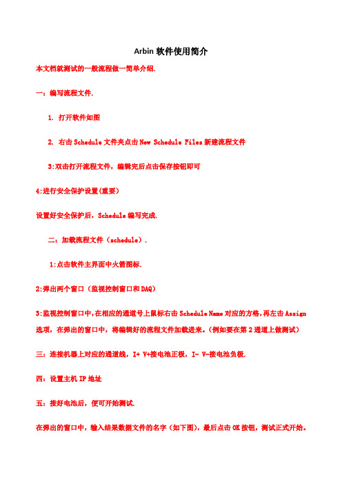
Arbin软件使用简介本文档就测试的一般流程做一简单介绍.一:编写流程文件.1.打开软件如图2.右击Schedule文件夹点击New Schedule Files新建流程文件3:双击打开流程文件,编辑完后点击保存按钮即可4:进行安全保护设置(重要)设置好安全保护后,Schedule编写完成.二:加载流程文件(schedule).1:点击软件主界面中火箭图标.2:弹出两个窗口(监视控制窗口和DAQ)3:监视控制窗口中,在相应的通道号上鼠标右击Schedule Name对应的方格,再左击Assign 选项,在弹出的窗口中,将编辑好的流程文件加载进来。
(例如要在第2通道上做测试)三:连接机器上对应的通道线,I+ V+接电池正极,I- V-接电池负极.四:设置主机IP地址五:接好电池后,便可开始测试.在弹出的窗口中,输入结果数据文件的名字(如下图),最后点击OK按钮,测试正式开始。
如果测试运行中,想要暂停测试,可以点击工具栏上的按钮。
暂停测试后,如果想恢复测试,那么点击按钮,在弹出的窗口中,点击OK按钮确认即可恢复测试.六:data watcher(查看数据)1:打开data watcher 2实时更新图形:3:设置坐标量程点击data实时显单击Chartsetting:Enable Zoom4:保存当前图形对当前图拍照截七:导出Excel表格1:单击Launch Excel单击Launch 2:单击Add-Ins3:单击Import Data 4:选择数据源和表格形式单击单击Import选择文设置输出路输出表5:表格导出完成控制类型介绍.1.搁置 rest.例搁置30秒(DV_Time≥1表示1秒钟采一个点):2.恒流充电或放电 Current(A)(正表示充电,负表示放电).例 1A充电至1A 放电至3.恒压 Voltage(V) (一般接在恒流之后使用)例恒压截止电流为.4.倍率充电或放电 C-Rate (正为充电,负为放电)例在第1通道做1Ah电池5倍率充电至测试做倍率测试,首先要在batch文件设置被测电池的容量.双击Batch Files 文件夹下面的文件,在对应的通道Capacity(Ah)填入被测电池容量.倍率测试其实可以直接用恒流来做,转化为相应的恒流即可.如1Ah的电池用5倍率充电,相当于用恒流1×5=5A 充电.5.恒功率充电或放电Power(W). (正为充电,负为放电).例 50W恒功率将电池充电至.50W恒功率将电池放电至.6.恒负载放电 Load(Ohm)例电池对10欧姆恒负载放电至7.设置循环 Set Variable(s)例第1步至第3步循环50次8.电流斜坡 Current Ramp(A) (注意斜率可正可负)例起始为1A,斜率为的电流斜坡对电池充电15秒.例秒时间,电流从1A上升到73A.这种情况的话,我们要自行计算它的斜率.dI/sec=(73-1)/=40有两种设定方法(推荐使用第2种,控制更稳定):9.电压斜坡 Voltage Ramp(V) (注意电压一般只为正)与电流斜坡基本一致,不再赘述.10.电流阶梯Current Staircase(A)例阶梯电流初始为1A,每3S增加2A,对电池充电15S.11.电压阶梯 Voltage Staircase(V)与电流阶梯基本一致,不再赘述.12.直流内阻 Intrenal Resistance例用振幅为5,脉宽为10ms的脉冲测内阻.如果将上述schedule中的Offset:0改为 Offset:3,则图像相对于X轴整体上移3个单位,如下图:13.恒流恒压 CCCV 和CCCP(建议使用CCCV)例恒流1A充至恒压,截止电流为.CCCP设置与CCCV一致,不再赘述.截止条件介绍.1.当前步运行时间 PV_CHAN_Step_Time例搁置15秒,就是说,该步以时间作为截止条件.2.当前电流值 PV_CHAN_Current (一般用于恒压作为截止条件)如恒压,截止电流为.3.当前电压值 PV_CHAN_Voltage(即当前电池电压)例 1A充电至或1A放电至4.当前测试时间 PV_CHAN_Test_Time (用得较少)从测试开始计时. 必须每步都添加此条件.例测试运行30分钟就停止,不管当前在运行那一步.(例子为充电,搁置,放电3步)注意Goto Step 项选的是End Test.点击下图中下拉菜单中的More,将有更多的截止条件.因为大都是不常用的,不一一介绍,如果需要用到,可电话或E-mail联系我们.采点条件介绍.1.按时间间隔采点 DV_Time例搁置15秒,每隔1秒采一个点.2.按电流的变化量采点 DV_Current例恒压,截止电流为,每1秒采一个点,另外,电流每增加或减少采一个点.3.按电压的变化量采点 DV_Voltage例恒流1A充至,每1秒采一个点,另外,电压每升高或降低采一个点.特别注意:在编写Schedule的时候,很多控制类型都要选择电流量程(Current Range)。
neusar使用手册
neusar使用手册
Neusar是一个功能强大的软件,它提供了许多功能和工具,以帮助用户更高效地管理和分析数据。
以下是Neusar的使用手册,包括安装、基本功能和高级功能的介绍。
1. 安装Neusar.
下载Neusar安装程序并双击运行。
按照安装向导的指示完成安装过程。
安装完成后,打开Neusar软件。
2. 基本功能。
数据导入,Neusar支持导入各种格式的数据,如CSV、Excel等。
用户可以通过简单的操作将数据导入到Neusar中。
数据管理,Neusar提供了数据筛选、排序、删除等功能,帮助用户更好地管理数据。
数据分析,Neusar内置了各种数据分析工具,用户可以通过这些工具进行数据分析和可视化。
3. 高级功能。
数据建模,Neusar支持数据建模和预测分析,用户可以利用这些功能进行复杂的数据分析。
数据挖掘,Neusar提供了数据挖掘工具,帮助用户发现数据中的隐藏模式和规律。
自定义功能,Neusar还支持用户自定义功能和脚本编程,用户可以根据自己的需求扩展Neusar的功能。
总结,Neusar是一款功能丰富的数据管理和分析软件,它提供了丰富的功能和工具,帮助用户更高效地进行数据管理和分析。
通过本使用手册的介绍,用户可以快速上手Neusar,并充分利用其强大的功能。
希望以上内容能够帮助你更好地了解Neusar软件的使用方法。
Arlequin操作说明解析
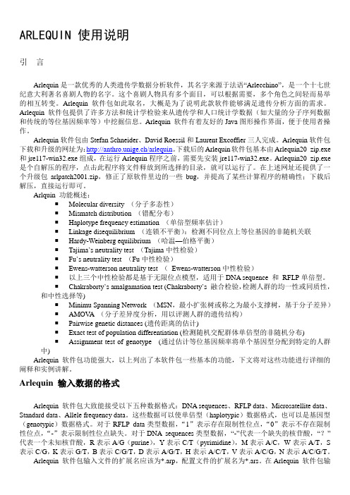
ARLEQUIN 使用说明引言Arlequin是一款优秀的人类遗传学数据分析软件,其名字来源于法语“Arlecchino”,是一个十七世纪意大利著名喜剧人物的名字。
这个喜剧人物具有多个面目,可以根据需要,多个角色之间轻而易举的相互转变。
Arlequin软件包如此取名,大概是为了说明此款软件能够满足遗传分析方面的需求。
Arlequin软件包提供了许多方法和统计学检验来从遗传学和人口统计学数据(如大量的分子序列数据和传统的等位基因频率等)中挖掘信息。
Arlequin 软件有着友好的Java图形操作界面,便于使用者操作。
Arlequin软件包由Stefan Schneider、David Roessil和Laurent Excoffier三人完成。
Arlequin软件包下载和升级的网址为:http://anthro.unige.ch/arlequin。
下载后的Arlequin软件包基本由Arlequin20_zip.exe 和jre117-win32.exe组成,在运行Arlequin程序之前,需要先安装jre117-win32.exe。
Arlequin20_zip.exe 是个自解压的程序,点击此程序将文件释放到所选择的目录,就可以运行了。
在上述网址还提供了一个升级包arlpatch2001.zip,修正了原软件里边的一些bug,并提高了某些计算程序的精确性;下载后解压,直接运行即可。
Arlquin 功能概述:Molecular diversity (分子多态性)Mismatch distribution (错配分布)Haplotype frequency estimation (单倍型频率估计)Linkage disequilibrium (连锁不平衡):检测不同位点上等位基因的非随机关联Hardy-Weinberg equilibrium (哈温—伯格平衡)Tajima`s neutrality test (Tajima中性检验)Fu`s neutrality test (Fu中性检验)Ewens-watterson neutrality test (Ewens-watterson中性检验)以上三个中性检验都是基于无限位点模型,适用于DNA sequence 和RFLP单倍型。
anaplan 手册

ANAPLAN是一个动态的规划平台,旨在帮助企业进行计划、预测和决策。
以下是ANAPLAN的一些关键特点和功能:
1.实时数据集成:ANAPLAN可以与各种数据源进行集成,包括数据库、CRM系
统和其他企业应用程序。
这使得用户可以轻松地获取最新的数据并进行计划和预测。
2.灵活性:ANAPLAN具有高度的灵活性,可以适应各种业务需求和行业。
用户
可以根据自己的需求定制数据模型、仪表盘和预测模型。
3.可视化工具:ANAPLAN提供一系列可视化工具,使用户能够直观地查看和分
析数据。
这有助于用户更好地理解数据并做出更好的决策。
4.协作功能:ANAPLAN支持多人协作,使团队成员可以共同制定计划和决策。
此外,ANAPLAN还提供了版本控制功能,确保数据的一致性和准确性。
5.定制化报告:用户可以根据自己的需求定制报告,以便更好地了解业务状
况、趋势和预测结果。
报告可以导出为多种格式,方便与其他团队成员共
享。
总的来说,ANAPLAN是一个强大的规划平台,可以帮助企业更好地进行计划、预测和决策。
通过实时数据集成、可视化工具、协作功能和定制化报告等功能,ANAPLAN可以帮助企业提高业务效率和准确性。
摩尔分析软件手册说明书

Software Manual MO.Affinity AnalysisContents1.System Requirements2.Term Definitions3.General Layout4.Saving and Exporting Data5.Analysis Setup in the Home Screen6.Data Selection7.Dose Response Fitpare ResultsThe MO.Affinity Analysis software allows straightforward analysis and evaluation of MicroScale Thermophoresis data. It allows quantification of binding parameters such as dissociation constants (K d) or EC50 values and easy comparison of results e.g. for one target protein binding to different compounds.The MO.Affinity Analysis software guides the user through all important steps from data selection to evaluation by using a clearly organized submenu layout in the task bar. Creating an analysis file will retain the chosen settings for data analysis. Additionally, the software allows inspection and exporting of both raw and processed data at any step during data analysis.This manual explains the main functions integrated in the MO.Affinity Analysis software.1. S ystem RequirementsIf the necessary licenses have been purchased, MO.Affinity Analysis software can be installed on computers meeting the following requirements:Operating system: Windows 7/10 Professional 64 bitCPU: Intel Core i5 or betterRAM: 8 GB or moreHard disk: 20 GB or more free disk space availableDisplay resolution: 1600 x 900 or betterSoftware: Microsoft .NET 4.5.1 framework (included in installer ofMO.Affinity Analysis software)Operating system language: English or GermanAn external computer mouse is necessary to access all software features.2. T erm DefinitionsTarget: The fluorescent molecule. The concentration of the target molecule is constant throughout a dilution series.Ligand: Non-fluorescent binding partner. The ligand concentration is varied by serial dilution.MST Trace: MST fluorescence signal overtime. A typical MST trace contains an initialdetection of the sample fluorescence (bydefault recorded for 3-5 seconds), followed byactivation of the MST power to induce thetemperature gradient and subsequentdetection of thermophoretic changes influorescence (by default recorded for 20-30 seconds). Finally, MST power isdeactivated and back diffusion of fluorescentmolecules is monitored (recorded for a shortperiod only).MST Run: A run includes a series of MST traces,typically of a fluorescent target molecule versus aserial dilution of a ligand.Merge Set: A series of replicates of MST runs, withidentical MST power, LED/excitation power as wellas target concentrations. Data within one Merge Setwill be averaged and error bars will be calculatedand displayed. Note that the ligand concentrationsdo not necessarily have to be identical and can varybetween merged MST runs.Analysis Set: A complete dataset consisting of a number of Merge Sets or single MST runs, for parallel analysis and direct comparison. Dose response curves of runs and Merge Sets in Analysis Sets can be compared in the same charts with the MO.Affinity Analysis software. All runs contained in one Analysis Set are analyzed with the same evaluation parameters.Analysis (file): A single Analysis Set, or a collection of Analysis Sets. The analysis can be saved at any time. An analysis file can be used to integrate a larger number of MST experiments for a comprehensive and systematic data analysis.Raw Data: All fluorescence data recorded by the Monolith instrument: MST traces, capillary scans and shapes, initial fluorescence values and bleaching rates. All raw data can be viewed in the Raw Data Inspection tool (see Figure 1 and section 3, point 6).Please note that the capillary scan displayed is the scan recorded before the MST measurement, not afterwards (applicable to MST measurements performed with MO.Control software).Figure 1: MST Raw Data Inspection: (A) Properties, (B) MST Traces, (C) Capillary Scan, (D) Capillary Shape, (E) Initial Fluorescence, (F) Bleaching Rate. Please note that the capillary scan displayed is the scan recorded before the MST measurement, not afterwards (applicable to MST measurements performed with MO.Control software).3. G eneral LayoutAll major functions of the MO.Affinity Analysis software are organized in the task bar:Four tabs guide the user through the process of MST data analysis:1. Home2. Data Selection3. Dose Response Fit4. Compare ResultsIt is recommended to complete all four steps in this order to ensure proper documentation and analysis of MST experiments. Movement between tabs during the analysis process is possible, e.g. to add additional files, edit names of Analysis sets, etc.Additional buttons in the task bar are:5. Quick saving of the analysis file.6. Raw Data Inspection is available at any time during the analysis process by selecting theRaw Data Inspection button on the top right of the window. This will open a separate window which displays all experiment-associated settings and meta-data, as well as detailed charts of raw MST traces, capillary scans, overlays of capillary shapes, initial fluorescence values and bleaching rates. Selected runs and traces will be highlighted in both, the MO.Affinity Analysis main window as well as in the Raw Data Inspection window. For detailed views of Raw Data Inspection options, see Figure 1.7. Alerts will be displayed on the top right of the main window. Alerts include experimentalinconsistencies as well as warnings about potential inconsistencies during data processing and fitting.Context-related supporting information, such as term definitions and equations, can be found when clicking the buttons located on each page.Anything you do in the software can be undone by pressing Ctrl + Z.4. S aving and Exporting DataThe MO.Affinity Analysis software allows for saving the current analysis at any time, using the drop-down menu in the top left (click ), the quick save button in the task bar or navigation back to the Home tab.Moreover, chart and tabular data can be exported where indicated using the export buttons (click ), which are located in the Dose Response Fit and Compare Results submenus as well as in the Raw Data Inspection section. Available image formats for export are .svg, .pdf and .png. Notethat .svg and .pdf contain vector graphics which can be processed by graphic editing software. Tabular data are saved in .xlsx or .csv format. Results can also be saved as a condensed report in .pdf format on the Dose Response Fit and Compare Results screens.5. A nalysis Setup in the Home ScreenIn the Home screen, create a new MST analysis or load a preexisting analysis file. Analysis files are saved in the .nta format. Changes in an analysis can be saved at any time.When creating a new analysis, enter an analysis name and optionally add comments, e.g. purpose of the analysis, assay conditions etc. Recently opened analysis files are listed chronologically. Start adding raw data to your analysis here, or in the next tab Data Selection.6. D ata SelectionSee Figure 2 for a summary of the options you have for Data Selection.To add MST runs to the analysis, use the drag-and-drop function for .ntp, .ntdb or .moc files, or use the load function to browse folders and select single or multiple files. MST runs of the selected file will appear in the Data Selection window as thumbnails of normalized MST Traces with a description of name, experiment settings and date. By changing the View option in the top panel, you can alter the presentation of the MST data thumbnails to Dose Response, Capillary Shape or Initial Fluorescence.Before data analysis is performed, choose the type of analysis. Toanalyze binding by MST, click on the MST button in the Choose AnalysisType panel. In cases of ligand-induced fluorescence changes where thefluorescence values of each capillary are used to determine bindingconstants, click the Initial Fluorescence button.Note: Use the Initial Fluorescence analysis if there is a ligand-concentration dependent change in sample fluorescence >±20 %. Referto the User Starting Guide or the MO.Control software for moreinformation.Note:The data points presented in the “Dose Response” thumbnail viewcorrespond to the F norm values determined after the MST powerdependent time intervals (see section 7).For further analysis and determination of binding parameters, MST runs are combined into Analysis Sets. Clicking the “Auto-Append” button will create a single Analysis Set which contains all loaded MST runs as independent single runs. Alternatively, MST runs can be added by clicking the symbol on the bottom right of each MST run thumbnail. This automatically creates a new Merge Set.To add replicate runs to a Merge Set, drag-and-drop them there directly. Merged runs will be displayed with average values and error bars in the Dose Response Fit screen. The software allows the merging of runs if the runs were collected using the same- LED/excitation power- MST power- Capillary type- Acquisition mode (fluorescence channel) and optics module (optics contained in a Monolith NT.Automated vs optics contained in a Monolith NT.115/NT.115Pico/belFree)Figure 2: Create Analysis and Merge Sets from MST runs in the Data Selection menu.Depending on the software used to perform the measurement, not all of these criteria may be saved in the file. As a result, it may not be possible to merge data collected with different software. When the user tries to add an incompatible run to a Merge Set, the software will reject the run and display an incompatibility message. To create a custom number of different Merge and Analysis Sets, drag-and-drop the MST run thumbnails.Hint: Analysis Sets and Merge Sets can also be rearranged by simple dragging and dropping.Please note that names of Merge and Analysis Set can be edited for better description and documentation by clicking the pen symbol on the respective flyout. The flyout appears upon mouse-over in the respective Analysis Set field (see screenshot below). Also, after an Analysis Set was created the analysis mode can still be switched between MST- and initial fluorescence analysis by selecting the respective button. Another button allows to switch to the expert mode for analysis (see next section for more details). Once Analysis Sets are created, binding data can be quantified.7. D ose Response FitThe Dose Response fit window allows for fitting MST data to obtain either dissociation constants (K d s, using the law of mass action) or EC50 values (using the Hill equation). In the window, normalized MST traces as well as corresponding dose response plots of the selected MST data are shown. Figure 3 summarizes the data analysis and fitting workflow.By selecting either an Analysis Set or a Merge Set on the left, the respective MST traces and their dose response plots are displayed. By default, F norm-values in the dose response plot are calculated from the ratio of normalized fluorescence F0/F1, where F0corresponds to the normalized fluorescence prior to MST activation. F1is by default determined after an optimal MST power-dependent time interval which yields the best signal-to-noise ratio.Use the mouse or the arrow keys to navigate through the analysis tree in the left panel. The right arrow key expands an Analysis Set or Merge Set, while the left arrow key collapses it.Data fitting is performed instantly after selecting the respective fit routine (K d Model or Hill Model). Fitting requires initial values, which are determined automatically by the software (shown as Guess values in the fit model). Known parameters, such as target concentration, need to be fixed by checking the Fix checkbox. In some cases it may be required to guide the fitting algorithm by manually entering initial Guess values.Note: The Hill fit should only be used if theinteraction involves a cooperative bindingmode. A 1:1 interaction should always be fittedusing the K d Model.After a fit is performed, a range of statisticalparameters is automatically calculated anddisplayed. For definitions, fit equations andmore information, click the button.Replicates within one Merge Set are displayedas average values and error bars representingthe standard deviation. Fits are applied to theaverage values. In order to get an errorestimation on the resulting K d, fit the replicatesindividually and use this data to performstatistics.For in-depth data evaluation and fit refinement, single runs and MST traces can be highlighted either by selection on the left, or by clicking on the respective MST trace or data point in the graphs. After highlighting, outliers can be excluded from the fit (either greyed out or invisible ).Figure 3: Analysis of binding constants and EC50-values.For a more in-depth evaluation of MST data, activate the Raw Data Inspection . Here, effects such as sample aggregation, adsorption to capillary walls or fluorescence intensity variations in the titration series can be easily identified. Please see the MO.Control software for more information on sample quality and assay optimization.When preparing Merge Sets for presentation that containnon-binding negative control interactions, move themouse cursor over the name of the Merge Set. A flyoutwill appear with a chain link symbol. Clicking this symbolinitializes all enabled fit parameters as nonbinder, whichmeans a horizontal line will be drawn through the pointsat their average value. This allows the comparison ofnonbinders with binders in the Compare Results view. Torevoke non-binder status, navigate to the data fittingsection of the respective run and untick all unneededcheckboxes.As an alternative to using the default analysis settings, the positions of F1 and F0 can be manually adjusted after enabling the Expert Mode for the Analysis Set (see Figure 4). Using this mode, the F1 and F0 cursors can be placed anywhere along the MST timetraces. The Expert Mode should only be used if the default analysis procedure did not yield satisfying results.Figure 4: Activation of the Expert Mode and visualization of different cursor settings.Similarly, when working with an Initial Fluorescence Analysis Set, the Expert Mode can be enabled to analyze ligand-dependent photobleaching effects (bleaching rate). Please contact your NanoTemper Technologies Support for more information.Chart visuals: Chart colors can be changed in the Data Selection, Dose Response Fit and Compare Results sections. All charts in the Dose Response Fit and Compare Results sections can be zoomed and adjusted for optimal visualization. Use the Zoom Extent button to adjust all data in the chart to the chart size. Zooming in-and-out of the chart is performed by scrolling the mouse wheel. Horizontal or vertical zooming can be performed by pressing shift or control on the keyboard while scrolling, respectively. Click and hold the mouse wheel and move the mouse to drag the chart (see Figure 5).Figure 5: Mouse control of chart visualization.8. C ompare ResultsThe Compare Results tab allows for a side-by-side comparison of MST runs and Merge Sets within an Analysis Set. In this tab, data and fitting results can also be exported in tabular and graphic format, including all binding data and the algorithms used. By selecting an Analysis Set on the left, all included data are plotted in the same chart. Selection of a Merge Set or a single MST run will highlight the selected experiments and grey-out the remaining experiments in the Analysis Set.Dropdown menus to change the Fit Model (K d or Hill) and display type (F norm, ∆F norm, Fraction Bound) are located on the top of the dose response chart. While the Fraction Bound normalization is best suited for a direct comparison of binding affinities, the ∆F norm normalization provides additional information about amplitude size and direction (please contact your NanoTemper Technologies Customer Support for more information). Both charts and chart raw data can be exported as an image file (.svg, .png or .pdf) or text file (.csv or .xlsx) for further use and external analysis.In addition to the visualization options, the Compare Results menu also includes a table summarizing number of averaged experiments (n), fit parameters, affinities and fit quality.Finally, the Generate Full Report button summarizes all charts and tables into one single PDF. Click the Generate Full Report button in the Dose Response Fit view to obtain a report even with unfitted data.ContactNanoTemper Technologies GmbHFloessergasse 481369 MunichGermanyPhone: +49 (0)89 4522895 0Fax: +49 (0)89 4522895 60***********************MicroScale Thermophoresis™ is a trademark.NanoTemper® and Monolith® are registered trademarks.NanoTemper® and Monolith® are registered in the U.S. Patentand Trademark Office.V10_2018-03-14。
Arlequin操作说明
Arlequin操作说明Arlequin操作说明1、引言1.1 系统概述1.2 目的1.3 预期读者1.4 文档范围2、系统要求2.1 软件需求2.2 硬件需求2.3 支持的操作系统3、安装Arlequin3.1 Arlequin3.2 安装过程3.3 配置选项4、创建新项目4.1 新建项目4.2 项目设置4.3 导入数据4.4 数据编辑5、运行分析5.1 选择分析类型 5.2 参数设置5.3 运行分析5.4 分析结果查看6、高级功能6.1 自定义分析6.2 脚本扩展6.3 数据处理和转换6.4 命令行模式7、常见问题解答7.1 安装问题7.2 数据导入问题7.3 分析结果解读8、附录8.1 附件一、Arlequin用户手册8.2 附件二、示例数据集8.3 附件三、数据规格说明注释:1、Arlequin:Arlequin是一种用于不同人群间基因样本分析的软件。
2、引言部分概述了本文档的目的、预期读者和范围。
3、系统要求部分列出了安装和运行Arlequin所需的软件、硬件和操作系统要求。
4、安装Arlequin部分提供了和安装软件的详细步骤。
5、创建新项目部分包括了新建项目、设置和导入数据的过程。
6、运行分析部分详细介绍了选择分析类型、设置参数、运行和查看分析结果的步骤。
7、高级功能部分提供了自定义分析、脚本扩展、数据处理和命令行模式的说明。
8、常见问题解答部分解答了一些用户经常遇到的问题。
9、附录部分提供了Arlequin用户手册、示例数据集和数据规格说明的附件。
附件:1、Arlequin用户手册:提供了更详细的Arlequin使用说明。
2、示例数据集:包含了用于演示各种分析功能的数据集。
3、数据规格说明:对Arlequin支持的数据规格进行了详细描述。
法律名词及注释:无。
medini analysis工具使用方法

medini analysis工具使用方法从头到尾地解释如何使用Medini Analysis工具。
[Medini Analysis]是一种功能强大的工具,可用于系统工程和软件开发。
它提供了一种集成的方式来建模、分析和验证系统,同时支持多种不同的建模语言和标准。
本文将介绍如何使用Medini Analysis工具,以便读者能够充分利用其功能和特性。
第一步:安装Medini Analysis要使用Medini Analysis工具,首先需要将其安装到计算机上。
用户可以从Medini Analysis官方网站上下载安装程序,并按照提示进行安装。
安装过程相对简单,只需几个步骤即可完成。
在安装完成后,用户可以启动Medini Analysis,并开始使用它的功能。
第二步:创建新项目在启动Medini Analysis后,用户可以选择创建一个新项目。
用户需要提供项目的名称和描述,并选择使用的建模语言和标准。
Medini Analysis支持多种建模语言,如UML、SysML和AUTOSAR,用户可以根据实际需要进行选择。
创建新项目后,用户可以开始向其中添加模型和设计。
第三步:建模和设计在新项目中,用户可以使用Medini Analysis提供的建模工具来创建系统模型和设计。
用户可以使用图形界面进行建模,也可以通过输入代码的方式来进行设计。
Medini Analysis支持多种建模工具和技术,用户可以根据自己的熟悉程度和需求进行选择。
建模和设计完成后,用户可以对模型进行分析和验证。
第四步:分析和验证Medini Analysis提供了丰富的分析和验证功能,用户可以使用这些功能来对系统模型进行分析和验证。
用户可以对模型进行静态分析,在设计阶段捕获潜在的问题和错误。
用户还可以对模型进行动态仿真,验证系统的行为和性能。
此外,Medini Analysis还支持模型检查和形式化验证,用户可以通过这些功能来验证系统的正确性和安全性。
Arlequin操作说明

ARLEQUIN 使用说明引言Arlequin是一款优秀的人类遗传学数据分析软件,其名字来源于法语“Arlecchino”,是一个十七世纪意大利著名喜剧人物的名字。
这个喜剧人物具有多个面目,可以根据需要,多个角色之间轻而易举的相互转变。
Arlequin软件包如此取名,大概是为了说明此款软件能够满足遗传分析方面的需求。
Arlequin软件包提供了许多方法和统计学检验来从遗传学和人口统计学数据(如大量的分子序列数据和传统的等位基因频率等)中挖掘信息。
Arlequin 软件有着友好的Java图形操作界面,便于使用者操作。
Arlequin软件包由Stefan Schneider、David Roessil和Laurent Excoffier三人完成。
Arlequin软件包下载和升级的网址为:http://anthro.unige.ch/arlequin。
下载后的Arlequin软件包基本由Arlequin20_zip.exe 和jre117-win32.exe组成,在运行Arlequin程序之前,需要先安装jre117-win32.exe。
Arlequin20_zip.exe 是个自解压的程序,点击此程序将文件释放到所选择的目录,就可以运行了。
在上述网址还提供了一个升级包arlpatch2001.zip,修正了原软件里边的一些bug,并提高了某些计算程序的精确性;下载后解压,直接运行即可。
Arlquin 功能概述:Molecular diversity (分子多态性)Mismatch distribution (错配分布)Haplotype frequency estimation (单倍型频率估计)Linkage disequilibrium (连锁不平衡):检测不同位点上等位基因的非随机关联Hardy-Weinberg equilibrium (哈温—伯格平衡)Tajima`s neutrality test (Tajima中性检验)Fu`s neutrality test (Fu中性检验)Ewens-watterson neutrality test (Ewens-watterson中性检验)以上三个中性检验都是基于无限位点模型,适用于DNA sequence 和RFLP单倍型。
polarr用法

polarr用法
Polarr是一款图像编辑应用程序,提供了广泛的编辑工具和功能,使用户可以对照片进行高级编辑和滤镜效果的应用。
Polarr的使用方法如下:
1. 下载和安装:在支持的设备上下载和安装Polarr应用程序。
2. 打开应用程序:打开Polarr应用程序后,您可以选择从设备相册导入照片,或使用摄像头拍摄新的照片。
3. 图像调整:在编辑选项卡中,您可以进行各种图像调整,如曝光度,对比度,色调,饱和度等。
您可以使用滑块或直接输入数值来调整参数。
4. 滤镜效果:Polarr提供了多种滤镜效果,您可以从预设列表中选择适合您照片的滤镜,并应用到图像中。
您还可以调整滤镜的强度和效果,以满足您的需求。
5. 高级编辑工具:除了基本的图像调整和滤镜效果外,Polarr 还提供了许多高级编辑工具,如曲线,色彩融合,去雾等。
这些工具允许您更精细地调整图像的特定部分,并创建个性化的效果。
6. 保存和分享:完成编辑后,您可以保存图像到设备相册,也可以直接分享到社交媒体平台或通过电子邮件发送给其他人。
通过这些简单的步骤,您可以使用Polarr进行照片编辑和增强,并创建出令人印象深刻的图像效果。
Aberlink 3D 软件教程
Aberlink 3D软件教程Rev. Dec 12, 2007Aberlink 3D 软件教程1.0 简介本教程旨在让使用者熟悉Aberlink 3D软件,并能利用软件所提供的功能进行工件的检测。
该教程从测量的基本概念讲起,包括机台归零、测针校正以及教学模型的检测,因此教学过程可分为几个部分,方便操作者理解和掌握。
2.0 开机&机台归零每次开机都需要执行机台归零,软件根据机台的零点确定探头的位置。
启动Aberlink 3D软件将会弹出如下提示:注意:如果测针不在行程的底端或者你无法支撑测针的重量,请不要点击“Yes”。
这是因为只有在机器行程的底端,力才是处在完全平衡的状态的。
如果当测针在行程的顶部时点击“Yes”,气浮开始漂浮,而测针则会由于自身的重力而脱落。
点击“Yes”后会弹出如下提示:点击“Yes”驱动系统将会启动,然后会出现如下窗体:当点击“OK“,机器会自动寻找参考点。
参考点的具体位置可能会随着机器的不同而不同,机器究竟向哪个方向移动去寻找参考点都是有软件设置决定的。
所以一定要确保测针是位于参考点正确的方向上。
Aberlink 3D的缺省设置是机器测量空间的右、后、上角。
因此机台归零的起始点可以位于测量空间的任何位置,但是不要距离零点太近。
归零过程结束后,窗体会自动隐藏。
3.0 测针校正软件无法探测机台目前究竟是用的是什么型号的测针以及测针的位置和方向,因此在开始测量之前一定要对测针进行校正。
校正之前,先将测针移动到校正球正上方约25mm的位置上。
3.1 使用旋转测针自动旋转测针标有A、B值,表示两个方向的旋转角度。
如果测针校正按钮显示的是星形测针标志(表示不可旋转测头)点击按钮左下角的测针图标:按钮的外观将会变为如下所示:点击A和B任何一个,将会出现测针数据窗口:窗口中的方格表示测针所能旋转到的各个角度。
A轴表示的竖直方向(0表示测针垂直向下)。
注意到所有的90度都显示为灰色。
editbin使用方法
editbin使用方法摘要:一、editbin简介二、editbin的使用方法1.安装和配置2.基本功能操作a.打开文件b.保存文件c.剪切、复制、粘贴功能d.查找和替换e.撤销和恢复操作3.进阶功能介绍a.批量处理文件b.脚本编写c.插件使用4.常见问题与解决方案5.总结与建议正文:editbin是一款实用的文本编辑器,它功能强大,操作简便,广泛应用于各种编程语言和文本处理任务。
本文将详细介绍editbin的使用方法,帮助读者更好地掌握这款工具。
一、editbin简介editbin是一款开源的文本编辑器,支持多种编程语言,如C、C++、Java、Python等。
它具有丰富的功能和快捷键,可以极大地提高编程效率。
二、editbin的使用方法1.安装和配置在官方网站下载适用于你操作系统的editbin版本,然后按照提示进行安装。
安装完成后,启动editbin,按照个人习惯配置快捷键、编辑器主题等。
2.基本功能操作(1)打开文件:在editbin中,点击“文件”菜单,选择“打开”,然后选择需要编辑的文件。
(2)保存文件:在编辑完成后,点击“文件”菜单,选择“保存”或“另存为”,选择保存路径和文件名。
(3)剪切、复制、粘贴功能:在编辑过程中,可以按Ctrl+X、Ctrl+C、Ctrl+V进行剪切、复制和粘贴操作。
(4)查找和替换:点击“编辑”菜单,选择“查找”或“替换”,输入需要查找或替换的内容,然后点击“查找下一个”或“替换全部”。
(5)撤销和恢复操作:在editbin中,可以按Ctrl+Z撤销操作,按Ctrl+Y恢复操作。
3.进阶功能介绍(1)批量处理文件:editbin支持批量处理多个文件,你可以将多个文件拖拽到editbin中,然后同时编辑多个文件。
(2)脚本编写:editbin支持脚本编写,你可以编写脚本实现一些复杂的操作,如自动格式化代码、自动完成等功能。
(3)插件使用:editbin支持插件扩展,你可以在官方网站下载相关的插件,如语法高亮、代码折叠等,以提高编辑体验。
用于药物研发的分子对接软件的使用技巧

用于药物研发的分子对接软件的使用技巧随着药物研发领域的发展和进步,计算机辅助药物设计的重要性日益凸显。
分子对接技术被广泛应用于药物研发中,可以预测化合物与受体的结合模式,从而指导新药分子的设计和优化。
而为了更好地进行分子对接研究,研究人员常常会使用一些专业的分子对接软件。
本文将介绍一些常见的用于药物研发的分子对接软件的使用技巧。
1. VinaVina是一种广泛应用的免费分子对接软件,它能够高效地进行分子对接计算。
以下是一些使用Vina的技巧:- 安装和配置:首先,需要从官方网站或源代码库中下载Vina软件,并按照安装指南进行安装。
然后,配置软件的运行环境,包括指定受体和配体分子的文件路径,并设置其他参数如计算网格的大小等。
- 导入受体和配体:使用Vina进行分子对接前,需要将受体和配体的结构文件导入到软件中。
一般情况下,受体和配体的文件格式是pdb或pdbqt。
- 设置搜索空间:Vina需要设置一个搜索空间,用于指定受体结构中比较有可能发生配体结合的区域。
通过定义一个接受区域的坐标范围,可以限制对接计算的搜索空间大小,提高计算效率。
- 运行对接计算:配置完毕后,即可运行Vina进行分子对接计算。
在计算过程中,软件会通过评分函数对每个配体进行评估,并给出一个分数,用于描述配体与受体结合的亲和性。
2. AutodockAutodock是另一种广泛应用于药物研发领域的分子对接软件,它提供了一套完整的分子对接计算流程,并具备良好的可视化功能。
以下是一些使用Autodock的技巧:- 导入受体和配体:在使用Autodock进行分子对接前,需要先将受体和配体的pdb文件导入到软件中。
此外,还可以对受体和配体进行处理,如添加氢原子、给配体加电荷等。
- 设置搜索空间:与Vina类似,Autodock也需要设置一个搜索空间以缩小对接计算的范围。
可以通过手动指定参考原子的坐标范围,或者利用软件提供的自动搜索功能找到合适的搜索空间。
Arlequin操作说明解析
ARLEQUIN 使用说明引言Arlequin是一款优秀的人类遗传学数据分析软件,其名字来源于法语“Arlecchino”,是一个十七世纪意大利著名喜剧人物的名字。
这个喜剧人物具有多个面目,可以根据需要,多个角色之间轻而易举的相互转变。
Arlequin软件包如此取名,大概是为了说明此款软件能够满足遗传分析方面的需求。
Arlequin软件包提供了许多方法和统计学检验来从遗传学和人口统计学数据(如大量的分子序列数据和传统的等位基因频率等)中挖掘信息。
Arlequin 软件有着友好的Java图形操作界面,便于使用者操作。
Arlequin软件包由Stefan Schneider、David Roessil和Laurent Excoffier三人完成。
Arlequin软件包下载和升级的网址为:http://anthro.unige.ch/arlequin。
下载后的Arlequin软件包基本由Arlequin20_zip.exe 和jre117-win32.exe组成,在运行Arlequin程序之前,需要先安装jre117-win32.exe。
Arlequin20_zip.exe 是个自解压的程序,点击此程序将文件释放到所选择的目录,就可以运行了。
在上述网址还提供了一个升级包arlpatch2001.zip,修正了原软件里边的一些bug,并提高了某些计算程序的精确性;下载后解压,直接运行即可。
Arlquin 功能概述:Molecular diversity (分子多态性)Mismatch distribution (错配分布)Haplotype frequency estimation (单倍型频率估计)Linkage disequilibrium (连锁不平衡):检测不同位点上等位基因的非随机关联Hardy-Weinberg equilibrium (哈温—伯格平衡)Tajima`s neutrality test (Tajima中性检验)Fu`s neutrality test (Fu中性检验)Ewens-watterson neutrality test (Ewens-watterson中性检验)以上三个中性检验都是基于无限位点模型,适用于DNA sequence 和RFLP单倍型。
aerdata 操作手册800字左右

Aerdata操作手册第一节:概述1.1 什么是AerdataAerdata是一款专业的航空数据分析工具,旨在帮助航空公司、飞机租赁公司和飞机制造商等行业实现对飞机数据的有效管理和分析。
1.2 Aerdata的功能Aerdata包含了包括飞行数据、维护数据、安全数据等在内的多种数据管理和分析功能,能够帮助用户全面了解飞机运行情况,提高运营效率和飞行安全。
第二节:安装与使用2.1 一般要求为了顺利安装Aerdata,您需要确保您的电脑系统符合以下基本要求:- 操作系统:Windows 7或更高版本- 内存:4GB或以上- 存储空间:20GB以上2.2 安装步骤1) 下载Aerdata安装程序2) 运行安装程序并按照提示完成安装2.3 使用步骤1) 打开Aerdata软件2) 输入用户名和密码并登入3) 在主界面选择您需要进行的操作,如数据查看、数据分析等第三节:数据管理3.1 数据录入Aerdata支持多种数据的录入,包括飞行数据、维护记录、安全报告等。
用户可以通过手动录入或导入文件的方式将数据导入系统。
3.2 数据查看Aerdata提供了直观的数据查看界面,用户可以通过筛选和排序等功能快速找到所需数据,并且可以以多种图表形式展示数据,方便用户进行数据分析。
3.3 数据分析Aerdata提供了强大的数据分析功能,用户可以通过设置不同的参数和模型,来对飞机数据进行深入分析,例如飞行效率、维护成本等指标。
第四节:报表输出4.1 报表生成Aerdata支持用户自定义报表模板,并能够根据用户需要自动生成报表,包括飞行数据报告、维护记录报告等。
4.2 报表导出用户可以将生成的报表导出为Excel、PDF等格式,方便共享和存档。
第五节:数据安全5.1 数据备份与恢复Aerdata自带数据备份和恢复功能,用户可以定期对数据进行备份,以防数据丢失或损坏。
5.2 数据权限管理Aerdata支持用户权限管理,管理员可以根据需要设置不同用户的操作权限,保证数据安全。
- 1、下载文档前请自行甄别文档内容的完整性,平台不提供额外的编辑、内容补充、找答案等附加服务。
- 2、"仅部分预览"的文档,不可在线预览部分如存在完整性等问题,可反馈申请退款(可完整预览的文档不适用该条件!)。
- 3、如文档侵犯您的权益,请联系客服反馈,我们会尽快为您处理(人工客服工作时间:9:00-18:30)。
Arbin软件使用简介
本文档就测试的一般流程做一简单介绍.
一:编写流程文件.
1.打开软件如图
2.右击Schedule文件夹点击New Schedule Files新建流程文件
3:双击打开流程文件,编辑完后点击保存按钮即可4:进行安全保护设置(重要)
设置好安全保护后,Schedule编写完成.
二:加载流程文件(schedule).
1:点击软件主界面中火箭图标.
2:弹出两个窗口(监视控制窗口和DAQ)
3:监视控制窗口中,在相应的通道号上鼠标右击Schedule Name对应的方格,再左击Assign选项,在弹出的窗口中,将编辑好的流程文件加载进来。
(例如要在第2通道上做测试)
三:连接机器上对应的通道线,I+ V+接电池正极,I- V-接电池负极. 四:设置主机IP地址
五:接好电池后,便可开始测试.
在弹出的窗口中,输入结果数据文件的名字(如下图),最后点击OK按钮,测试正式开始。
如果测试运行中,想要暂停测试,可以点击工具栏上的按钮。
暂停测试后,如果想恢复测试,那么点击按钮,在弹出的窗口中,点击OK按钮确认即可恢复测试.
六:data watcher(查看数据)
1:打开data watcher 2实时更新图形:
3:设置坐标量程点击data wacther
实时显示
4:保存当前图形
七:导出Excel表格1:单击Launch Excel 对当前图拍照截图
单击Chart setting: Enable Zoom setting可以对图形进行放大或缩小。
单击X1 Axes可以对坐标轴的量程进行设置。
2:单击Add-Ins 3:单击Import Data 单击Launch Excel
单击Add-Ins
4:选择数据源和表格形式5:表格导出完成单击Import Data
选择文件
设置输出路径输出表格
控制类型介绍.
1.搁置rest.
例搁置30秒(DV_Time≥1表示1秒钟采一个点):
2.恒流充电或放电Current(A)(正表示充电,负表示放电).
例1A充电至4.2V
1A 放电至2.5V
3.恒压Voltage(V) (一般接在恒流之后使用)
例 4.2V恒压截止电流为0.05A.
4.倍率充电或放电C-Rate (正为充电,负为放电)
例在第1通道做1Ah电池5倍率充电至4.2V测试
做倍率测试,首先要在batch文件设置被测电池的容量.
双击Batch Files 文件夹下面的ArbinSys.bth文件,在对应的通道Capacity(Ah)填入被测电池容量.
倍率测试其实可以直接用恒流来做,转化为相应的恒流即可.
如1Ah的电池用5倍率充电,相当于用恒流1×5=5A 充电.
5.恒功率充电或放电Power(W). (正为充电,负为放电).
例50W恒功率将电池充电至4.2V.
50W恒功率将电池放电至2.5V.
6.恒负载放电Load(Ohm)
例电池对10欧姆恒负载放电至2.5V
7.设置循环Set Variable(s)
例第1步至第3步循环50次
8.电流斜坡Current Ramp(A) (注意斜率可正可负)
例起始为1A,斜率为0.5的电流斜坡对电池充电15秒. 例 1.8秒时间,电流从1A上升到73A.
这种情况的话,我们要自行计算它的斜率.
dI/sec=(73-1)/1.8=40
有两种设定方法(推荐使用第2种,控制更稳定):
9.电压斜坡Voltage Ramp(V) (注意电压一般只为正)
与电流斜坡基本一致,不再赘述.
10.电流阶梯Current Staircase(A)
例阶梯电流初始为1A,每3S增加2A,对电池充电15S.
11.电压阶梯Voltage Staircase(V)
与电流阶梯基本一致,不再赘述.
12.直流内阻Intrenal Resistance
例用振幅为5,脉宽为10ms的脉冲测内阻.
如果将上述schedule中的Offset:0改为Offset:3,则图像相对于X轴整体上移3个单位,如下图:
13.恒流恒压CCCV 和CCCP(建议使用CCCV)
例恒流1A充至4.2V 恒压,截止电流为0.05A.
CCCP设置与CCCV一致,不再赘述.
截止条件介绍.
1.当前步运行时间PV_CHAN_Step_Time
例搁置15秒,就是说,该步以时间作为截止条件.
2.当前电流值PV_CHAN_Current (一般用于恒压作为截止条件)
如恒压4.2V,截止电流为0.05A.
3.当前电压值PV_CHAN_Voltage(即当前电池电压)
例1A充电至4.2V
或1A放电至2.5V
4.当前测试时间PV_CHAN_Test_Time (用得较少)
从测试开始计时. 必须每步都添加此条件.
例测试运行30分钟就停止,不管当前在运行那一步.(例子为充电,搁置,放电3步)
注意Goto Step 项选的是End Test.
点击下图中下拉菜单中的More,将有更多的截止条件.
因为大都是不常用的,不一一介绍,如果需要用到,可电话或E-mail联系我们.
采点条件介绍.
1.按时间间隔采点DV_Time
例搁置15秒,每隔1秒采一个点.
2.按电流的变化量采点DV_Current
例恒压4.2V,截止电流为0.05A,每1秒采一个点,另外,电流每增加或减少0.1A采一个点.
3.按电压的变化量采点DV_Voltage
例恒流1A充至4.2V,每1秒采一个点,另外,电压每升高或降低0.1V采一个点.
特别注意:
在编写Schedule的时候,很多控制类型都要选择电流量程(Current Range)。
有些电流要经过计算才能知道大小,以选择合适的量程,这点需留意.
机器名牌上有电流3个档位的量程,如:
------------------------------------------------------------------------------------------------
Channel# 丨High 丨Medium 丨Low 丨Voltage
-------------------------------------------------------------------------------------------------
1-40 丨±10A 丨±1A 丨±10mA 丨0-5V
-------------------------------------- -----------------------------------------------------------
其中,高量程为±10A,即-10到﹢10A.
中量程为±1A,即-1到﹢1A.
低量程为±10mA,即-10mA到﹢10mA.
比如用1A充电,虽然可以选择高量程或中量程,但是尽可能的选择较低的量程,可以提高精度.。