Tutorial_1
FT41-Tutorial1-letter-Chinese - 副本
,滚动项目标签才可得到‘)图标在 Flotherm 中,所有的几何图形的彩色都是有特定含义的。
当只看到绿色边框而看不到任何几何体时,这表明所有几何体被压入 assembles(组件)中。
组件(Assemblies)会象目录存放文件一样可存放几何体。
此几何模型包括一个含有3个通风孔的机箱.如在项目管理器中所示,这些通风孔由一些打孔的板覆盖。
监控点置于箱子中心,它作为数字热电偶跟踪求解过程中的温度变化(或任何其它变量),要获取某特定位置上指定的物理量,这是更简便的方法。
(换到全屏视图模式。
使用鼠标将当前的命令模式从选择模式切换到操作模式当处于操作模式可打开调色板并实现对它的开要创建几何体,需要点击图标将其切换至选择模式(将‘手’转点击绘图板上部的图标,这样就只有视图: Snap to Grid : Snap to Object: Free Snap。
这时鼠标指针将变为十字此几何体不是固体,而是可透过空气的物体。
在这一模型中,我100W的热量直接扩散到指定的空间。
中选中这个几何体,点击图标前选中多个物体,则在对话框中将显示所有物这一模型就有了一个新的文件名。
现在开始计算。
点击求解图标求结果过程中会出现收敛曲线(Profiles)窗口,以便监控求解过程。
本次求解会在约75次迭代后收敛。
,打开。
由于平面图参数主现在,使用平移,缩放,旋转工具来操作图形,在操作模式变为图标。
或使用热键备注:当鼠标指针设在‘Selection mode’(选择模式)下时,您还可以通过使用键盘上的左右箭头键在模型中移动观察面。
Tutorial 1 Matlab 命令窗口的使用

Tutorial 1 Matlab 命令窗口的使用一、命令窗口的基本操作命令窗口(Command Window)位于MATLAB 操作桌面的右方,如图1所示,用于输入命令并显示除图形以外的所有执行结果,是MATLAB 的主要交互窗口。
命令窗口可以从MATLAB 操作桌面中分离出来,以方便单独显示和操作,也可以重新返回操作桌面中,其他窗口也有相同的操作。
分离命令窗口可选择菜单命令Desktop→Unlock Command Window,也可单击窗口右上角的按钮,还可以使用鼠标将命令窗口拖离操作桌面,分离的命令窗口如图2 所示。
如将命令窗口返回操作桌面,可选择命令窗口的菜单命令Desktop→Dock Command Window,或单击窗口右上角的按钮。
在MATLAB 命令窗口中可以看到有一个“>>”,该符号为命令提示符,表示MATLAB 正在处于准备状态。
在命令提示符后输入命令并按回车键后,MATLAB 就会解释执行所输入的命令,并在命令后面给出计算结果。
图1 Matlab默认操作窗口图2 分离的命令窗口二、命令窗口的使用一般来说,一个命令行输入一条命令,命令行以按回车键结束。
但一个命令行也可以输入若干条命令,各命令之间以逗号分隔;若前一命令后带有分号,则逗号可以省略。
例程如下。
输入并执行以下内容。
以上两个例子都是在一个命令行输入3 条命令,不同的是两条命令之间的分隔符不同,一个是逗号,一个是分号。
可以看出,一条命令后如果带一个分号,则该命令执行结果不显示。
再看一个例子。
在命令窗口中输入以下内容。
表示输入数组A 和B。
比较可以看出,在输入数组的时候,分号有换行的作用。
在MATLAB 中,同一个符号在不同的命令中有不同的作用,后面的章节会有详细介绍。
有时候会碰到这样的情况,一个命令行很长,一个物理行之内写不下,可以在第一个物理行之后加上3 个小黑点(…)并按回车键,然后接着下一个物理行继续写命令的其他部分。
tutorial_1 soluation

Hardware Macstuff Winstuff 200 100
Software 1000 1500
In this economy the firm whose opportunity cost of producing a good is lowest is said to have a comparative advantage (CA) in producing that good. The firm with an absolute advantage (AA) in producing a good produces that good with the least amount of resources. Opportunity cost of producing 1 unit of: Hardware Macstuff Winstuff 5 units of software 15 units of software Software 1/5 units of hardware 1/15 units of hardware
Question 3 There are two firms: Macstuff and Winstuff. Each firm can produce either software or hardware using their resources. With one unit of its own resources Macstuff can produce 200 units of hardware or 1000 units of software. With one unit of its own resources Winstuff can produce 100 units of hardware or 1500 units of software. Each firm has 10 units of resources to allocate to the production of software and hardware. Suppose Macstuff and Winstuff agree to specialise their production according to their comparative advantage in producing software and hardware, and to then exchange with each other. Identify the bounds on the terms at which they would agree to trade software for hardware? Express your answer in terms of the amount of hardware that would be ‘paid’ for software. Explain your answer.
PSCAD_tutorials_1_4
PSCAD BASIC TRAININGTutorials 1 – 4Getting Started and Basic FeaturesTutorial 1Getting familiar – creating cases and librariesT1.1 Create a new case by using either the Menu or Toolbar . A new case should appear in the Workspace settings entitled noname [psc]. Right-click on this Workspace settings entry and select Save As… and give the case a name.NOTE: Do not use any spaces in the name!Create a folder called c:……/PscadTraining/Tutorial_01. Save the case as case01.pscT1.2 Open the main page of your new case. Build a case to compute the product of two input signals.21X X Y ⋅=t Sin X ⋅⋅⋅=10051 52=XYou may use the wire mode to connect different components Wire Mode.T1.3 Plot the output Y. Name the plots. Use X-Y plot feature to plot Y vs. X1 and X1 vs. X2.T1.4 Unload the above case and create a new library by using either the Menu or Toolbar . A new library should appear in the Workspace settings entitled noname [psl]. Right-click on this Workspace setting sentry and select Save As… and give the library a name.Save the case as case01.psl in c:……/PscadTraining/Tutorial_01T1.5 Under the Component Definitions branch, Copy the Component Definition called Multiplier from the Master Library into your new library. Rename the definition [my_mul] and enter a new description. Create an Instance of this definition and paste it into the main page of the new library. You have now created a new Component Definition!T1.6 Unload case01.psc and reload it. Save it as case02.psc . Replace the multiplier with the new component that you just created. Run the case to verify results. Modify the new component so that the output Y is()212X X Y ⋅⋅=Run the case and observe results.T1.7 Unload all cases except the master library. Load case02.psc and try to run the case. Now load case02.psl and try to run case02.psc.Unload and reload case02.psc. Now run the case!Tutorial 2Getting Familiar with PSCAD: Plots, Graphs & Curves and single line diagramsT2.1 In your …Program Files/pscad/examples/tutorial directory, open the case project called simpleac.psc. Set the case Plot Step to 50 μs and run the case. Using the Zoom feature, zoom into the area where the fault occurs. Get familiar with keyboard shortcuts.Save the case as simpleac01.psc in c:……/PscadTraining/Tutorial_02T2.2 Invoke the cross hairs mode and follow the curves with the cross hairs. Monitor all phases A, B and C by switching between curves using the ‘space bar’. Turn cross hairs off, zoom out to the previous view and resize if necessary. Get familiar with the ‘graph properties’ ‘graph frame properties’ and keyboard short cuts.T2.3 Right-click on the top graph and select Graph Properties. Invoke the cross hairs and flip between curves. Experiment with grid lines, markers, colors and line thickness. Is it presently possible to have curves of different thickness on the same graph?T2.4 Plot the Phase A sending end and receiving end currents on the same graph.T2.5 Convert the circuit of the sending end to a single line format.Save the case as simpleac02.psc in c:……/PscadTraining/Tutorial_02T2.6 Convert the transmission line interface component in the receiving end to single line format. Use the’ breakout’ component to link single line drawings to three phase drawings.T2.7 Measure the line to ground voltage on the sending end. Use the ‘data tap’ to derive the three voltage signals from the voltmeter connected to the ‘single’ line. Plot the voltages.Rerun the case, starting from a S napshot file, taken at 0.2 s.Note that the timed fault logic and timed breaker logic settings are not changed in the simulation. However, the fault appears to be initiated at 0.05 s and not 0.25s as specified. Why? Can the time axis scale be changed to reflect the ‘actual’ time?Can the simulation time step be changed when the case is run from a snapshot file?T2.8 Resize the page and add sticky notes and experiment with curve settings. Make the page look ‘presentable’ in a report. Go to edit=> workspace settings and check out the available options.Tutorial 3Building a simple caseT3.1 Create a new case by using either the Menu or Toolbar. A new case should appear in the Workspace settings entitled noname [psc]. Right-click on this Workspace settings entry and select Save As… and give the case a name. NOTE: Do not use any spaces in the name!).Save the case as accircuit01.psc in c:……/PscadTraining/Tutorial_03T3.2 Open the main page of your new case. Construct the circuit as shown below using the methods discussed up until now.T3.3 Use the Three Phase Source model and externally control it using a Real Constant tag for frequency and a Slider to control L-G Peak Voltage. Create a Plot and monitor currents Ia, Ib and Ic flowing through the Three Phase Breaker. Set the Timed Breaker Logic for 1 operation and so that the breaker is initially closed and will open at 0.4 sec.Externally control the Three Phase Fault with a Dial. Initiate the fault at 0.1 sec., with duration of 0.2 sec. Run the case multiple times, each time trying a different Fault Type.Experiment with different fault and breaker times. What happens when the series inductors are all set to 0.5 H? Why?T3.4 Your supervisor asks you to monitor the fundamental +\-\0 sequence currents flowing through the breaker during each fault: Use the On-Line FFT component for this as shown to the right. Run the case again multiple times, each time trying a different Fault Type. Does zero sequence current flow for every type of fault?T3.5 Add a Three Phase RMS Voltage meter between the breaker and the fault branch. Set the Voltage for Per-Unitizing to the voltage specified in your source. Why is voltage ripple sometimes present? What happens when you adjust the Smoothing Time Constant of the RMS meter?Save the case as accircuit01.psc in c:……/PscadTraining/Tutorial_03T3.6 Construct a Sequence of Events, which performs exactly the same timed control logic you are using now for your breaker and fault. When you are finished, delete the Fault Logic and Timed Breaker Logic components and provide the required control signals from your Sequencer.Save the case as accircuit02.psc in c:……/PscadTraining/Tutorial_03T3.7 Create a page module and move the Three Phase Fault component, along with the Dial, inside of it. HINT: The sub-page will require 3 electrical nodes (X-Nodes) and one data input node.Save the case as accircuit03.psc in c:……/PscadTraining/Tutorial_03T3.8 Measure the Harmonic impedance of this system at different points. Use the ‘Harmonic Impedance’ meter and get the instructor to explain how it is used.Open the case as accircuit04.psc in c:……/PscadTraining/Tutorial_03. Run the case and see the output files created from the ‘Harmonic Impedance’ component.T3.9 EXTRA: Create a data signal to monitor the A Phase fault current by defining it as an “Internal Output Variable” in the Three Phase Fault Component dialog window. Add Output Channels and create a plot inside the Page Component to monitor the signal. Cut the entire Plot window and Paste it into the Main Page of the case and run it again. What happens?T3.10 EXTRA: Output the Phase A fault current through an Export Tag to the main page. HINT: You must modify the Page Component.Tutorial 4Series tuned filterT4.1 Create a new case by using either the Menu or Toolbar . A new case should appear in theWorkspace settings entitled noname [psc]. Right-click on this Workspace settings entry and select Save As… and give the case a name. NOTE: Do not use any spaces in the name!). Save the case as tunedfilt01.psc in c:……/PscadTraining/Tutorial_04T4.2 Open the main page of your new case. Construct the circuit as shown below using the methods discussed until now:T4.3 Add a File Reference to point to a file called signal.out in your course directory. To view the file, double-click the File Reference icon. Signal.out will be the input file for the File Read component. NOTE: The file signal.out is an output file created by PSCAD and is located on your course disk. The two columns of data represent time and signal magnitude, which has an AC fundamental frequency, along with 5th and 7th harmonics.T4.4 Use the File Read component to input an external signal to the Single Phase Source , as shown in the diagram above. Under File Name in the File Read dialog window, enter signal.out and change the number of columns to read to 2. Set the Single Phase Source to Ideal , DC and External Input . Set the default variable R, L and C values to 0.1 Ω, 0.07036 H and 100 μF respectively.T4.5 In the Project Settings dialog window set the simulation time to 0.15 sec and time and plot step to 50 μs. Run the case and plot the signals Vin and Vout as curves on the same graph. The series filter is tuned by default to pass only one frequency. What frequency does the signal Vout appear to be? HINT: Use markers- mode on the graphT4.6 Revert back to standard startup (that is, remove starting from a snapshot). Add the Multiple Run component and set it up to sequentially vary the capacitance of the capacitor from 10 μF to 100 μF (in 10 μF increments). Connect the Multiple run output to the capacitor as shown to the right. NOTE : Make sure the Multiple Run component is enabled!T4.7 Run the case and monitor Vin and Vout . What affect does the varying capacitance have on the output voltage?T4.8 Use the feature in Multiple Run to analyze Vin . Find the value of C that would give the minimum Vin .T4.9 EXTRA : Using components from the CSMF section of the Master Library to calculate the resonant frequency in Hz for each new value of capacitance C.CL 21f 0⋅⋅π⋅=T4.10 EXTRA : Check the impedance spectrum using the ‘Harmonic Impedance’ component.。
新核心大学英语听说教程1uni

Before listening to the audio, try to predict the type of answer that will be given, such as a fact, opinion, or explanation. This can help you focus on relevant information and filter out irrelevant details.
• Enhance speaking skills: Students will practice speaking in different contexts, including making presentations, participating in discussions, and giving speeches.
模仿发音
通过模仿英语母语者的发音,提高自己的口语 流利度和准确性。
口语表达
通过回答问题、复述故事、描述图片等方式, 训练口语表达能力。
口语交流
与英语母语者进行口语交流,提高实际应用能力。
Role playing and group discussions
Positioning key information and filtering irrelevant information
Identifying important details
While listening, identify important details that are relevant to the question or task. This may include specific information, names, dates, or numbers.
新编英语教程1unit1

04
提前阅读问题,了解需要回答 的内容和要求。
在听的过程中,注意捕捉关键 信息和细节,记录重要内容。
根据问题类型,选择合适的答 题方法,确保答案准确、完整
。
Listening skills sharing
预测答案
根据问题和听力材料的主题,预测可能的答案。
筛选无关信息
在听的过程中,快速筛选出与问题相关的信息,忽略无关内容。
04
reading comprehension
Reading article analysis
文章主题分析
文章结构分析
文章语言特点分析
文章逻辑关系分析
本篇文章主要探讨了英语学习 的技巧和方法,包括词汇、语 法、阅读和写作等方面的学习 建议。
文章采用了总分总的结构,先 总体介绍了英语学习的重要性 ,然后分别从词汇、语法、阅 读和写作四个方面进行了详细 阐述,最后总结了提高英语学 习的关键因素。
Analysis of Listening Materials
词汇量
评估听力材料中涉及的词 汇量,确定是否超出了学 生的词汇范围。
FT41-Tutorial1-letter-Chinese
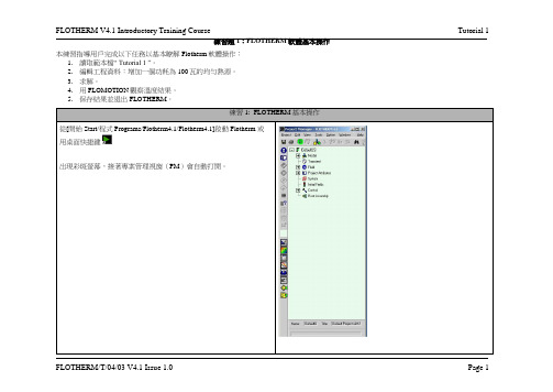
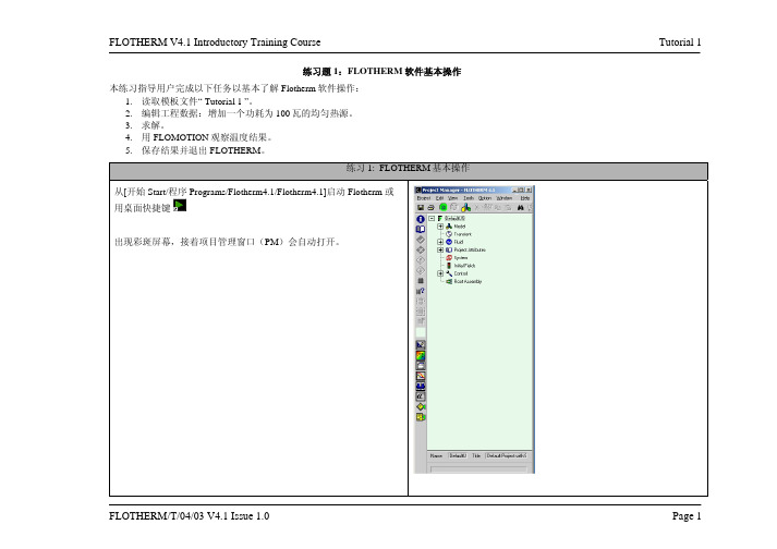
練習題1:FLOTHERM軟體基本操作本練習指導用戶完成以下任務以基本瞭解Flotherm軟體操作:
1.讀取範本檔“ Tutorial 1 ”。
2.編輯工程資料:增加一個功耗為100瓦的均勻熱源。
3.求解。
4.用FLOMOTION觀察溫度結果。
5.保存結果並退出FLOTHERM。
,滾動項目標籤才可得到‘
)圖示
此幾何模型包括一個含有3個通風孔的機箱.如在專案管理器中所示,這些通風孔由一些打孔的板覆蓋。
監控點置於箱子中心,它作為數字熱電偶跟蹤求解過程中的溫度變化(或任何其他變數),要獲取某特定位置上指定的物理量,這是更簡便的方法。
切換到操作模式 (
後,執行以下操作:
可打開調色板並實現對它的開
要創建幾何體,需要點擊圖示將其切換至選擇模式(將‘手’轉
(或使用熱鍵
視圖模式圖示
: Snap to Grid : Snap to Object: Free Snap 從繪圖板中的調色板中選擇幾何體。
這時滑鼠指標將變為十字
備註:您無需以科學計數法的形式輸入各項的值。
您還可以通過使用
此幾何體不是固體,而是可透過空氣的物體。
在這一模型中,我
100W的熱量直接擴散到指定的空間。
中選中這個幾何體,點擊圖示
備註:若在單擊圖示前選中多個物體,則在對話方塊中將顯示所有
現在開始計算。
點擊求解圖示
觀看結果,單擊視覺化圖示
中單擊建立視覺化平面圖標
:
將指標由圖示
變為圖示
或使用熱鍵
(選擇模式)。
简明英语测试教程第一章

简明英语测试教程第一章Simple English Test Tutorial Chapter 1This chapter serves as a concise guide to help learners prepare for their English language tests. The following sections will provide valuable tips and strategies for each section of the test, including listening, reading, writing, and speaking.Section 1: Listening SkillsDeveloping strong listening skills is crucial for success in any English language test. To enhance your listening abilities, consider the following techniques:1.1 Active ListeningEngage actively while listening to audio samples or conversations. Focus on understanding the key points, main ideas, and supporting details. Take notes if necessary to better retain the information.1.2 Practice ListeningListen to a wide range of English materials such as music, podcasts, and movies. Attempt to comprehend the context and meaning behind the words. Regular practice will sharpen your listening skills.Section 2: Reading SkillsThe reading section is designed to assess comprehension and vocabulary skills. To improve your performance in this section, take note of the following tips:2.1 Skimming and ScanningLearn to skim and scan passages quickly to identify the main ideas and locate specific information within the text. This technique helps save time during the test.2.2 Vocabulary ExpansionExpand your vocabulary by reading different genres and topics. Make a habit of using context clues to deduce the meaning of unfamiliar words. This practice will allow you to understand and answer questions more effectively.Section 3: Writing SkillsThe writing section evaluates your ability to express ideas, organize thoughts, and use correct grammar and vocabulary. Here are some suggestions to enhance your writing skills:3.1 Plan and StructureBefore starting your essay, take a few minutes to outline the main points and structure. This provides a clear direction for your writing and ensures a logical flow of ideas.3.2 Grammar and VocabularyReview essential grammar rules and practice using a variety of sentence structures. Expand your vocabulary by learning synonyms and idiomatic expressions to add depth to your writing.Section 4: Speaking SkillsThe speaking section assesses your ability to communicate fluently and coherently. To improve your speaking skills, incorporate the following strategies:4.1 Pronunciation and IntonationWork on correct pronunciation and intonation to enhance your overall fluency. Practice listening to and imitating native speakers as this will greatly improve your oral communication skills.4.2 Practice SpeakingEngage in conversations with native or proficient English speakers as much as possible. Join discussion groups, take part in speaking clubs, and utilize language exchange platforms to gain confidence and fluency.ConclusionMastering the English language requires consistent practice and dedication. By focusing on each section of the test - listening, reading, writing, and speaking - and utilizing the techniques provided in this tutorial, you can enhance your test performance and achieve success. Remember, regular practice and exposure to the language are key to progress and improvement.(Note: The given topic is "Simple English Test Tutorial Chapter 1". The format used is a tutorial-style format, providing tips and strategies for each section of the test.)。
G03W入门辅导-1(试用版)

G03W 的安装、初始化 和作业启动
2010试用版
G03 的主要计算功能
可用来预测气相和液相条件下,分子和化学反应的性质 :
• • • • • • • • • • •
分子的能量和结构 过渡态的能量和结构 振动频率 红外和拉曼光谱 热化学性质
外部的分子结构 3D浏览器
主窗口显示格式的初始化设置
点击“Display”按钮,弹出“Display Preferences”对话框。一般只须设置
输出字体,其余项目可用缺省设置
点击 “Output Font”按钮, “字体”建议选取“Courier New”
Courier New 是等宽 字体,可使输出数据 的显示整齐美观
挥效率和计算容量)
安装位置
建议将G03W安装于D或E盘。理由:保护程序文件及积累的输
入、输出和有用的中间文件。万一须格式化C:\ 盘时不致丢失
按此处置,在Windows系统重装后G03W也不必重装
软件安装:
启动Setup.exe,按屏幕提示输入软件的“Serial Number”并设 定安装路径,自动完成安装。
打开指定的 外部编辑器
用指定外部编辑器 浏览或编辑 当前作业输出文件
File 下拉菜单的命令
点击“File”打开下拉菜单
在线创建新作业 打开一个输入文件 修改旧的输入文件 程序的初始化设置
在Process拉菜单的命令
点击“Process”打开下拉菜单
启动批处理作业 暂停当前作业 当前Link后暂停 恢复运行当前作业 终止当前作业 本作业结束后 终止批处理 立即终止批处理
tutorial1matlab命令窗口的使用

Tutorial 1 Matlab 命令窗口的使用一、命令窗口的基本操作命令窗口(Command Window)位于MATLAB 操作桌面的右方,如图1所示,用于输入命令并显示除图形以外的所有执行结果,是MATLAB 的主要交互窗口。
命令窗口可以从MATLAB 操作桌面中分离出来,以方便单独显示和操作,也可以重新返回操作桌面中,其他窗口也有相同的操作。
分离命令窗口可选择菜单命令Desktop→Unlock Command Window,也可单击窗口右上角的按钮,还可以使用鼠标将命令窗口拖离操作桌面,分离的命令窗口如图2 所示。
如将命令窗口返回操作桌面,可选择命令窗口的菜单命令Desktop→Dock Command Window,或单击窗口右上角的按钮。
在MATLAB 命令窗口中可以看到有一个“>>”,该符号为命令提示符,表示MATLAB 正在处于准备状态。
在命令提示符后输入命令并按回车键后,MATLAB 就会解释执行所输入的命令,并在命令后面给出计算结果。
图1 Matlab默认操作窗口图2 分离的命令窗口二、命令窗口的使用一般来说,一个命令行输入一条命令,命令行以按回车键结束。
但一个命令行也可以输入若干条命令,各命令之间以逗号分隔;若前一命令后带有分号,则逗号可以省略。
例程如下。
输入并执行以下内容。
以上两个例子都是在一个命令行输入3 条命令,不同的是两条命令之间的分隔符不同,一个是逗号,一个是分号。
可以看出,一条命令后如果带一个分号,则该命令执行结果不显示。
再看一个例子。
在命令窗口中输入以下内容。
表示输入数组A 和B。
比较可以看出,在输入数组的时候,分号有换行的作用。
在MATLAB 中,同一个符号在不同的命令中有不同的作用,后面的章节会有详细介绍。
有时候会碰到这样的情况,一个命令行很长,一个物理行之内写不下,可以在第一个物理行之后加上3 个小黑点(…)并按回车键,然后接着下一个物理行继续写命令的其他部分。
OpenSim Tutorial1 for 30 and 31

OpenSim Tutorial #1Introduction to Musculoskeletal ModelingScott Delp, Allison Arnold, Samuel HamnerNeuromuscular Biomechanics LaboratoryStanford UniversityI.O BJECTIVESIntroduction to OpenSimModels of the musculoskeletal system enable one to study neuromuscular coordination, analyze athletic performance, and estimate musculoskeletal loads. OpenSim is open-source software that allows users to develop, analyze, and visualize models of the musculoskeletal system, and to generate dynamic simulations of movement [1]. In OpenSim, a musculoskeletal model consists of rigid body segments connected by joints. Muscles span these joints and generate forces and movement. Once a musculoskeletal model is created, OpenSim enables users to study the effects of musculoskeletal geometry, joint kinematics, and muscle-tendon properties on the forces and joint moments that the muscles can produce. With OpenSim, our goal is to provide a framework that allows the biomechanics community to create, share, and extend a library of models and dynamic simulation tools.PurposeThe purpose of this tutorial is to introduce users to OpenSim by demonstrating the utility of graphics-based musculoskeletal modeling and illustrating how muscle-tendon lengths and moment arms depend upon limb configuration. In this tutorial, you will:•Become familiar with OpenSim’s graphical user interface (GUI)•Discover some limitations of musculoskeletal models•Explore differences between “1-joint” (uni-articular) and “2-joint” (bi-articular) muscles •Use OpenSim to address an important clinical problemFormatEach section of the tutorial guides you through certain tools within OpenSim’s GUI and asks you to answer a few questions. The menu titles and option names you must select and any commands you must type to run OpenSim will appear in bold face. The questions can be answered based on information from OpenSim and basic knowledge of the human musculoskeletal system. As you complete each section of the tutorial, feel free to explore OpenSim and the lower extremity model further on your own. Depending on the amount of exploration you do, this tutorial will take about 1-2 hours to complete.Introduction to the OpenSim GUIThere are several key components of the OpenSim GUI that will be referred to throughout the tutorial. The table below will introduce you to these GUI components.GUI ComponentsTitleScreenshotToolbarMotion Text BoxMotion Slider / Video ControlsView WindowNavigator WindowCoordinates WindowProperties WindowII.M USCULOSKELETAL M ODEL OF THE L OWER E XTREMITYIn this section, you will load a model of the lower extremity [2] into OpenSim and make the model “walk.” The model represents an adult subject with an approximate height of 1.8 m and an approximate mass of 75 kg. The model consists of 13 rigid body segments and includes the lines of action of 86 muscles (43 per leg).Loading a ModelThe first model you will analyze is entitled Both Legs with Muscles. To load this musculoskeletal model into OpenSim:•Click the File menu and select Open Model.•Find the Models folder, which is located under your OpenSim installation directory, e.g., C:\OpenSim 3.0.Note: There are several different example models and motions in the Models folder. All of the model and motion files used in the remainder of the tutorial will be located in this Models folder.•Open the BothLegs folder, select the file BothLegs.osim, and click Open.After loading a model, its name will appear in the Navigator window. To see the Navigator window, which also provides specific information about the bodies, muscles, and joints in the model, click the Window menu and select Navigator. To expand a Navigator heading, click the plus icon to its left.Note: If already opened, you can also view the Navigator window by clicking its title bar.Viewing & Animating a ModelOpenSim allows you to orient the model using your mouse.R OTATE To rotate the view, click and hold the left mouse button and drag the mouse.T RANSLATE To translate the view, click and hold the center mouse button and drag the mouse. Z OOM To zoom, click and hold the right mouse button.To zoom in, drag the mouse down. To zoom out, drag the mouse up.In addition to your mouse, there are six orienting icons located along the right side of the View window. To view the model in the –X direction, click the icon. Similarly, click on the other icons to view along the other principal directions. To see the axes of the world reference frame, click the axes icon located on the right side of the View window.CoordinatesThe Coordinates window contains sliders that correspond to joint coordinates in the model. To see the Coordinates window, click the Window menu and select Coordinates. For the current model, the orientation of the pelvis corresponds to the orientation of the model.Note: If already opened, you can also view the Coordinates window by clicking its title bar.•The first three sliders correspond to rotations of the pelvis about the Z, X, and Y-axes of the “pelvis” reference frame. To rotate the pelvis about the Z-axis, drag the rZ slider.Similarly, to rotate the pelvis about the other two axes, drag the corresponding slider.Note: These rotations are different than rotating the model view.•The remaining sliders correspond to joint rotations and control a single degree of freedom.To rotate the joints, drag the sliders or type in a desired joint angle in the adjacent textbox.•To save a pose, or a specific set of joint coordinates, for later use in the tutorial:-Restore the default joint coordinates by clicking the Poses button and selecting Default.-Flex the right hip 45º by typing 45 into the r_hip_flexion textbox and pressing Enter.-Click the Poses button, select New, type r hip flex 45 in the textbox, and click OK.Loading a MotionTo animate the model, you need to load an associated motion file into OpenSim.•Click the File menu and select Load Motion. Ensure you are in the BothLegs directory, select the file BothLegsWalk.mot, and click Open. This motion file describes a normal gait.After loading a motion, its name will appear in the motion textbox,located on the toolbar. Additionally, a new branch will appear inthe Navigator titled Motions. Expand it to see all motions loadedfor a particular model, as shown.Motion SliderThe motion slider corresponds to the current motion file. To make the model “walk”, drag the motion slider. To animate the model, use the video control buttons, e.g., click play . There are also buttons to loop , pause , and control the speed of the animation.Questions1.Degrees of Freedome the Coordinate slider to view the degrees of freedom of the model. How manydegrees of freedom does the model have? List them.b.All models are approximations. Compare the degrees of freedom in the model to thedegrees of freedom in your lower limbs. Which motions have been simplified? Which motions have not been modeled at all?c.How many muscles are in the model? Is this greater than the number of degrees offreedom? What is the minimum number of muscles required to fully actuate the model?Hint: Full actuation of the knee, for example, means both knee flexion and knee extension.2.Muscle Pathsa.Muscle-tendon paths are represented in OpenSim by a series of points connected by linesegments. To see a list of all the muscles:•In the Navigator, expand the Forces, Muscles, and all headings.•To display a single muscle, right-click on a specific muscle name under the all group,e.g., GMED1, and select Display > Show Only from the popup menu.•To toggle the display of all muscles, double-click on the Muscles or all heading.Note: Double-clicking on a body, muscle group, or muscle heading in the Navigator toggles its display.In this model, the gluteus medius is represented by multiple lines of action (e.g., GMED1, GMED2, GMED3).Name two other muscles in the model that are represented with multiple lines of action.Why do you think these muscles are represented in this way?Hint: Other muscles with multiple lines of action use the same naming convention as the gluteus medius.b.For some muscles, two points, the muscle origin and insertion, are sufficient to describethe muscle path. For other muscles that wrap over bones or are constrained by retinacula, intermediate wrapping or via points must be defined. To view these wrapping points:•Zoom in on the right knee joint.•Hide all other muscles except the r knee extensors muscle group.•Fully flex the right knee using the r_knee_angle Coordinates slider.Notice that wrapping points are introduced in some of the knee extensors at certain knee angles, such that the muscles appear to wrap around the bones.Which knee extensor muscles have wrapping points? At what knee angle do they occur?3.Modeling LimitationsSome muscles in the lower limb model pass through the bones or deeper muscles at extreme ranges of motion. Zoom in on the right hip, and display only the GMAX3 muscle (r hip extensors group). Examine this muscle for the full range of hip flexion angles.Do you see any problems with GMAX3? In what ways are point-to-point representations of muscle paths a simplification of musculoskeletal geometry?III.J OINT A NGLES,M USCLE-TENDON L ENGTHS,&M OMENT A RMSIn this section, you will investigate how muscle-tendon lengths and moment arms depend onlimb configuration. Musculoskeletal geometry is very important to the function of muscles andto the development of quantitative musculoskeletal models. Muscle-tendon forces depend uponthe muscle-tendon length, and joint moments depend upon both muscle-tendon forces and moment arms. Therefore, accurate specification of musculoskeletal geometry is essential in developing an accurate model for predicting muscle-tendon forces and joint moments.Using the PlotterOpenSim’s Plotter allows you to plot muscle-tendon properties, such as length, moment arm, force, and joint moment. To generate a plot of fiber-length vs. knee angle for the rectus femorisand vastus intermedius muscles:•Return the model to its original pose by clicking Poses > Default in the Coordinates window.Note: Plots are created for the current configuration of the model. Your plots will be made for the default pose.•To open a new plot, click the Tools menu and select Plot. In the plotter window, click the Y-Quantity button and select fiber-length. This variable will appear on the y-axis.•After selecting an appropriate Y-Quantity, you must select the muscles for which you want to generate curves. Click on the Muscles button and a menu will appear.•To find muscles more quickly, you can filter the muscles by muscle group. Choose the model option and use the group drop down menu to select r knee extensors. The muscles list should now only show the muscles in the right knee extensors group.•Select rectus femoris and vastus intermedius from the list by clicking the checkboxeslabeled RF and VASINT.Note: You do not have to close the muscles window as long as the plotter window is open, and your selections are immediately updated in the Muscles textbox. This can be helpful when creating multiple curves on the same plot, which you will do in a few more steps.•Click X-Quantity and select r_knee_angle. This variable will appear on the x-axis.•To add a title to the plot, click the Properties button and type Fiber-Length vs. Knee Angleinto the textbox named Text under the Title tab. Explore the plot properties, and then click OK.•To add the curves to the plot, click Add.Note: The plots use the following SI units: meters (length), Newtons (force), Newton-meters (moment).•Do not close the plot window, as you will be adding more curves in the next section.Questions4.Muscle Fiber Length vs. Joint Anglea.Study the plot of muscle fiber length vs. knee angle. Do you think these curves wouldlook different if, for example, the right hip was flexed?b.You will now flex the right hip by recalling the pose you previously saved:•In the Coordinates window, click Poses and select your saved pose (r hip flex 45).•To add curves for 45º hip flexion using the same Quantities and Muscles, click Add.Note: To print or save a plot, right-click on the plot and select Print or Export Image.Compare the two sets of curves you have just plotted. How have the curves changed?Can you explain your findings? How can bi-articular muscles complicate analysis?5.Muscle Moment Arm vs. Joint AngleNow plot knee extension moment arm vs. knee angle for the same two muscles:•Return the model to its original position by clicking Poses >Default.•To delete the previous curves, select all the names from the Curves List and click Delete.Note: To select multiple curve names, hold down ctrl while selecting.•Click Y-Quantity, select moment arm, and r_knee_angle.•To add curves using the same Muscles and X-Quantity as previously selected, click Add.Note: If you hover the cursor over a curve, a tool tip will give the coordinates at that particular point.Study the plot of knee extension moment arm vs. knee angle for rectus femoris and vastus intermedius. At what knee angles do the moment arms peak? What are the peak moment arms?You may notice that the moment arm curves have a discontinuity. At what knee angle does the discontinuity occur? What do you think causes this?Hint: Look at Question 2.bOnce you have answered these questions, you can close the current plotter.Feel free to make more plots for other limb positions, muscles, and/or joints. When you are ready to continue with the tutorial, close the plotter window and close the Both Legs with Muscles model by clicking the File menu and selecting Close Model. Do not save the model settings to file.IV.A SSESSMENT OF H AMSTRINGS L ENGTH D URING C ROUCH G AITIn this final section of the tutorial, you will use OpenSim to investigate a possible cause of crouch gait, one of the most common walking abnormalities among individuals with cerebral palsy. It is characterized by excessive flexion of the knee during stance phase, which is often accompanied by exaggerated flexion and internal rotation of the hip. One hypothesized cause of crouch gait is short hamstrings, and orthopaedic surgeons will sometimes lengthen the hamstrings of such patients in an attempt to improve their posture and gait. However, other causes of excessive knee flexion are possible (e.g. weak ankle plantarflexors), and lengthening the hamstrings can compromise the strength of these muscles [3]. How can a surgeon determine whether a hamstring lengthening procedure is warranted?One possible way to judge whether a patient’s hamstrings are shorter than “normal” is to developa musculoskeletal model and compare the length of the hamstrings during the patient’s crouch gait cycle to the length of the hamstrings during a normal gait cycle. Suppose that an orthopaedic surgeon has brought you some kinematic data for a patient who walks with a crouch gait. The surgeon is contemplating whether to operate, and wants your opinion.File PreparationFollow these steps to load the crouch gait and normal gait files:•Load the model file SeparateLegs.osim. This model is located in the directory Models/SeparateLegs. Separate Legs with Muscles is similar to Both Legs with Muscles, except that it has separate left and right pelvis segments that connect to the sacrum.Note: All of the tutorial models and motions are relative to your OpenSim installation directory, e.g., C:\Program Files\OpenSim 3.0.•To rename a loaded model, right-click on the model name in the Navigator and select Rename from the popup menu. Type SepLegsCrouch into the textbox and click OK.Note: Renaming in this way does not affect the actual file name of the model.•Load the motion file crouch1.mot, which is in the same folder as the SeparateLegs model.This motion contains crouch gait data.•OpenSim has the ability to load multiple models simultaneously. To open a second model, load the SeparateLegs.osim file again.Note: If you do not see both models after loading, press the r key.•To rename the second model, right-click on the current model name and select Rename.Type SepLegsNormal into the textbox and click OK.Note: Throughout the rest of the tutorial, these two models will be referred to as crouch and normal.The second model you loaded automatically becomes the current model. Notice that the non-current model becomes translucent. Any action, such as loading a motion, will be applied only to the current model. You can change the position of the model in the viewer, by right-clicking on the model’s name and choosing Model Display Offset.•Making sure that the normal model is still current, load thesecond motion file normal.mot. This motion file containsnormal gait data.•OpenSim can synchronize multiple motions, allowing you toanimate multiple models simultaneously. To do this, expandthe Motions branch of each model in the Navigator, holddown ctrl (ctrl + command on a Mac), and select bothmotions names such that each name is highlighted. Right-click on either motion name, then select Sync. Motions fromthe popup menu, as shown.Questions6.Range of MotionTo animate the models and visually compare the crouch gait data to the normal gait data, click play. Notice that both motions are synchronized, as shown. Be sure to loop the animation, adjust the play speed, and rotate the models. What differences do you observe?Now quantitatively compare knee flexion angles over the crouch and normal gait cycles.•In a new plot, click Y-Quantity, select normal_gait(Deg.)…, and select r_knee_angle.Click OK.•Click X-Quantity and select normal_gait. Click OK.•Edit the text in the Curve Name textbox to read Normal Gait.•To add the curve of right knee angle vs. gait cycle, click Add.•Make the crouch model current by right-clicking on its name in the Navigator window and then select Make Current.•In the same plotter window, click Y-Quantity, select crouch1_gait(Deg.)…, and select r_knee_angle. Click OK.•Click X-Quantity and select crouch1_gait. Click OK.•In the Curve Name textbox edit the text to read Crouch Gait, then click Add.Can you identify the intervals at which heel strike, stance, toe off, and swing phase occur for a “normal” gait cycle?Sketch a plot of the curve, and label the intervals.What is the “normal” range of knee flexion during stance phase?How does this knee flexion curve for crouch gait compare to the normal gait data?7. Hamstrings LengthTo address the surgeon’s question, compare the hamstrings length over the crouch gait cycle tothe hamstrings length over the “normal” gait cycle.•To delete the previous curves, select all the names from the Curves List and click Delete.Note: To select multiple curve names, hold down ctrl while selecting.•Make the normal model current by right clicking on it in the Navigator window and then selecting Make Current•Click Y-Quantity and select muscle-tendon length.•Click on Muscles and select Hamstrings from the list. Click Close.Note: To quickly find the Hamstrings, type ham into the pattern textbox.•Click X-Quantity and select normal_gait(Deg.).•In the Curve Name textbox edit the text to read Normal Gait.•To add the curve of hamstrings length vs. gait cycle, click Add.•To make a similar curve for the crouch gait data, make the crouch model current. Then, click on Y-Quantity and re-select muscle-tendon length.•Click on Muscles and select Hamstrings.•Click X-Quantity and select crouch1_gait(Deg.).•In the Curve Name textbox, edit the name to read Crouch Gait, and then click Add.Study the curves. Based on the plot, what recommendation would you give the surgeon? Canyou think of any limitations of your analysis?8.Additional Crouch Gait Files (optional)The orthopaedic surgeon cares for three other patients who walk with a crouch gait. Repeat theabove analysis for motion files crouch2.mot, crouch3.mot, and crouch4.mot. Note that you can associate more than one motion with a model. Would your recommendations to the surgeon beany different for these patients? If you would like to learn more about this type of analysis,please read reference [3].References1.Delp, S.L., Anderson, F.C., Arnold, A.S., Loan, P., Habib, A., John, C.T., Guendelman, E., Thelen, D.G.OpenSim: Open-source software to create and analyze dynamic simulations of movement.IEEE Transactions on Biomedical Engineering, vol. 55, pp. 1940-1950, 2007.2.Delp, S.L., Loan, J.P., Hoy, M.G., Zajac, F.E., Topp E.L., Rosen, J.M. An interactive graphics-basedmodel of the lower extremity to study orthopaedic surgical procedures. IEEE Transactions on BiomedicalEngineering, vol. 37, pp. 757-767, 1990.3.Arnold, A.S., Liu, M., Ounpuu, S., Swartz, M., Delp, S.L., The role of estimating hamstrings lengths andvelocities in planning treatments for crouch gait, Gait and Posture, vol. 23, pp. 273-281, 2006.。
DotSpatial_Tutorial_1

Working with DotSpatial controlsTutorial (1)Purpose of this tutorial: Become familiar with the DotSpatial map control and its following functionalities: ZoomIn, ZoomOut, Zoom to Extent, Select, Measure, Pan, Info, and load data.This tutorial has 5 important steps.Step 1: Download the DotSpatial class libraryStep 2: Add the DotSpatial reference and change the compile option.Step 3: Add the DotSpatial Controls into the Visual Studio Toolbox.Step 4: Design the GUI. (GUI - Graphical User Interface)Step 5: Write the code for implementing the map operations.Step 1: Download the DotSpatial class library1. Download the DotSpatial class library (x86 Framework 4.0.zip) from the following URL.Step 2: Add the DotSpatial reference and change the compile option.2.1) Add the DotSpatial reference1. Right click over the project on the solution explorer and select the add reference from the context menu.2. Add the following 4 references from the downloaded folder. fig.5DotSpatial.Controls.dll, DotSpatial.Data.dll, DotSpatial.Data.Forms.dll, DotSpatial.Symbology.dllfig.5.2.2) Change the compile option from .Net FrameWork 4 Client Profile to .Net FrameWork 41. Right click over the project on the solution explorer and select the properties from the context menu.fig.6.Choose the Advanced Compile Options on the above window. fig.6fig.7. Select the .Net Framework 4 and save the project.fig.8 C#.net application change compile options.Step 3: Add the DotSpatial Controls into the Visual Studio Toolbox.3.1) Creating a new Tab on the ToolBox window and adding the DotSpatial class library.Create a new project in VB or C# and select the ToolBox on the standard menu bar. Right click on the ToolBox window and choose "Add Tab" from the context menu. Fig.1 Enter the new tab name as DotSpatial. On the DotSpatial tab right click and select the choose items from the context menu.fig.1.Click the Browse button on the Choose Tool Box Items window. fig.2.fig.2.Select the DotSpatial.Controls.dll from the downloaded folder. (fig.3)fig.3Make sure the AppManager is checked on the Choose Toolbox Items window. fig.4fig.4.Step 4: Design the GUI. (Graphical User Interface)Design the GUI as follows:Map Controlfig.9.Interface design considerations.1. Add 2 panel controls on the form.1.1) Name the first panel as pnlOperations and set the dock property as Top.1.2) Name the second panel as pnlMap and set the dock property as Fill.2. Drag the map control on to the pnlMap from the tool box, under the DotSpatial tab. Set the dock property of map to Fill.3. Add a group box on to the pnlOperations and name it as grbOperations.4. Create ten buttons inside the group box.4.1) Set the buttons properties as follows:4.2) Use shortcut keys for the button click event. Ex: Load Map button's short cut key is Shift + L. To implement this feature, on the properties window of the button select the Text property and use the & sign in front of any letter. In the load button case, Text property should be &L oad Map5. Add a title label above the group box. Name of the label should be lblTitle and the text property of the label is Basic Map Operations.Step 5: Write the code for implementing the map operations.1.Add the following namespaceVB'Required namespaceImports DotSpatial.ControlsC#//Required namespaceusing DotSpatial.Controls;2.Double click over the button on the form to get the selected button's click event code view.VBPrivate Sub btnLoad_Click(ByVal sender As System.Object, ByVal e As System.EventArgs) Handles btnLoad.Click'AddLayer() method is used to add a shapefile in to mapcontrolMap1.AddLayer()End SubPrivate Sub btnRemove_Click(ByVal sender As System.Object, ByVal e As System.EventArgs) Handles btnClear.Click'Clear() method is used to clear the shapelayers from mapcontrolyers.Clear()End SubPrivate Sub btnZoomIn_Click(ByVal sender As System.Object, ByVal e As System.EventArgs) Handles btnZoomIn.Click'ZoomIn method is used to ZoomIn the shape fileMap1.ZoomIn()End SubPrivate Sub btnZoomOut_Click(ByVal sender As System.Object, ByVal e As System.EventArgs) Handles btnZoomOut.Click'ZoomOut method is used to ZoomIn the shape fileMap1.ZoomOut()End SubPrivate Sub btnZoomToExtend_Click(ByVal sender As System.Object, ByVal e As System.EventArgs) Handles btnZoomToExtend.Click'ZoomToMaxExtent method is used to Extent the shape fileMap1.ZoomToMaxExtent()End SubPrivate Sub btnMeasure_Click(ByVal sender As System.Object, ByVal e As System.EventArgs) 'Measure function is used to measure the distance and areaMap1.FunctionMode = DotSpatial.Controls.FunctionMode.MeasureEnd SubPrivate Sub btnInfo_Click(ByVal sender As System.Object, ByVal e As System.EventArgs) Handles btnInfo.Click'Info function is used to get the information of the selected shapeMap1.FunctionMode = End SubPrivate Sub btnMeasure_Click_1(ByVal sender As System.Object, ByVal e As System.EventArgs) Handles btnMeasure.Click'Measure function is used to measure the distance and areaMap1.FunctionMode = FunctionMode.MeasureEnd SubPrivate Sub btnSelect_Click(ByVal sender As System.Object, ByVal e As System.EventArgs) Handles btnSelect.Click'Select function is used to select a shape on the shape fileMap1.FunctionMode = FunctionMode.SelectEnd SubPrivate Sub btnNone_Click(ByVal sender As System.Object, ByVal e As System.EventArgs) Handles btnNone.Click'None function is used to change the mouse cursor to defaultMap1.FunctionMode = FunctionMode.NoneEnd SubPrivate Sub btnPan_Click(ByVal sender As System.Object, ByVal e As System.EventArgs) Handles btnPan.Click'Pan function is used to pan the mapMap1.FunctionMode = FunctionMode.PanEnd SubC#private void btnLoad_Click(object sender, EventArgs e){//AddLayer method is used to add shape layersmap1.AddLayer();}private void btnClear_Click(object sender, EventArgs e){//ClearLayers method is used to remove all the layers from the mapcontrol map1.ClearLayers();}private void btnZoomIn_Click(object sender, EventArgs e){//ZoomIn method is used to ZoomIn the shape filemap1.ZoomIn();}private void btnZoomOut_Click(object sender, EventArgs e){//ZoomOut method is used to ZoomIn the shape filemap1.ZoomOut();}private void btnZoomToExtent_Click(object sender, EventArgs e){//ZoomToMaxExtent method is used to Extent the shape filemap1.ZoomToMaxExtent();}private void btnPan_Click(object sender, EventArgs e){//Pan function is used to pan the mapmap1.FunctionMode = FunctionMode.Pan;}private void btnInfo_Click(object sender, EventArgs e){//Info function is used to get the information of the selected shapemap1.FunctionMode = ;}private void btnMeasure_Click(object sender, EventArgs e){//Measure function is used to measure the distance and areamap1.FunctionMode = FunctionMode.Measure;}private void btnSelect_Click(object sender, EventArgs e){//Select function is used to select a shape on the shape filemap1.FunctionMode = FunctionMode.Select;}private void btnNone_Click(object sender, EventArgs e){//None function is used to change the mouse cursor to defaultmap1.FunctionMode = FunctionMode.None;}3. To display the tool tip message for the buttons, add the following code in the form load event. Double click over the form for getting the form load event code view.VBPrivate Sub Form1_Load(ByVal sender As System.Object, ByVal e As System.EventArgs) Handles MyBase.LoadDim btnToolTip As New ToolTip()btnToolTip.SetToolTip(btnLoad, "Shift + L")btnToolTip.SetToolTip(btnZoomIn, "Shift + I")btnToolTip.SetToolTip(btnZoomOut, "Shift + O")btnToolTip.SetToolTip(btnClear, "Shift + C")btnToolTip.SetToolTip(btnZoomToExtend, "Shift + E")btnToolTip.SetToolTip(btnPan, "Shift + P")btnToolTip.SetToolTip(btnInfo, "Shift + F")btnToolTip.SetToolTip(btnMeasure, "Shift + M")btnToolTip.SetToolTip(btnSelect, "Shift + S")btnToolTip.SetToolTip(btnNone, "Shift + N") End SubC#private void frmTutorial1_Load(object sender, EventArgs e){ToolTip btnToolTip = new ToolTip();btnToolTip.SetToolTip(btnLoad, "Shift + L");btnToolTip.SetToolTip(btnZoomIn, "Shift + I");btnToolTip.SetToolTip(btnZoomOut, "Shift + O");btnToolTip.SetToolTip(btnClear, "Shift + C");btnToolTip.SetToolTip(btnZoomToExtent, "Shift + E"); btnToolTip.SetToolTip(btnLoad, "Shift + L");btnToolTip.SetToolTip(btnInfo, "Shift + f");btnToolTip.SetToolTip(btnMeasure, "Shift + M");btnToolTip.SetToolTip(btnSelect, "Shift + S");btnToolTip.SetToolTip(btnNone, "Shift + N");btnToolTip.SetToolTip(btnPan, "Shift + N");}fig.10. Project Output for state shape file.。
FT41-Tutorial1-letter-Chinese
Tutorial 1
在 PM 中点击绘图板(DB)图标
。
绘图板 (DB)窗口占用右边屏幕,显示模型的四个视图. 重调尺寸并移 动 项目管理窗口 (PM)把它放在 DB 的左边,两个窗口同时可见。
在 Flotherm 中,所有的几何图形的彩色都是有特定含义的。当只看到 绿色边框而看不到任何几何体时,这表明所有几何体被压入 assembles (组件)中。组件(Assemblies)会象目录存放文件一样可存放几何 体。
或使用热键 F11 切换至视图选择模式。点住温度场 通过点击图标 平面(位于求解域中心)上的任意箭头并沿箭头轴向拖动鼠标。在平 面通过模型移动的过程中,软件会连续地更新并显示面板上的参数。 使用‘Legend’和‘Values’,察看温度结果。 点击 Legend Editor(色标编辑器)图标 将调出‘Legend Editor’对 话框。从 scalar(标量)下拉菜单中选择“Temperature(温度)”显 示温度色彩刻度。 单击“user(用户)”按钮激活滚轮(wheel), 这将允许你调整刻度表的范围。 完成后关闭对话框。 使用‘Values’观测值,用热键‘y’从正 Y 方向观测几何体。点击 ‘Value Dialog’观测值对话框图标 。 备注:当鼠标指针设在‘Selection mode’(选择模式) 下时,您还可 以通过使用键盘上的左右箭头键在模型中移动观察面。
Tutorial 1
出现彩斑屏幕,接着项目管理窗口(PM)会自动打开。
FLOTHERM/T/04/03 V4.1 Issue 1.0
Page 1
FLOTHERM V4.1 Introductory Training Course
练习 1: FLOTHERM 基本操作 在 PM 中点击[Project/New]并选择标签‘Tutorials’。注意:必须点 击图标 ,滚动项目标签才可得到‘Tutorials’标签。 选中项目文件“Tutorial 1”,点击‘OK’。
COSWORKS Tutorial 1

在这一章中将按部就班地为您演示线性静态分析功能。
⏹第1课: 一个托架体的分析⏹第2课: 一个装配曲柄的分析⏹第3课: 一个薄托架的分析(壳模型)⏹第4课: 一个I型梁的分析(壳模型)⏹第5课: 一个漏斗的分析(壳模型)⏹第6课: 一个燃料储存箱的分析(壳模型)⏹第7课: 在一个轴力作用下的滑轮分析⏹第8课: 一个带孔板的应力集中⏹第9课: 使用偏转载荷第1课: 一个托架体的分析在这课中,您将会学习到:⏹ 如何载入一个物体并建立一个静态分析项目, ⏹ 如何赋给物体材料,⏹ 如何插入约束并施加压力载荷, ⏹ 如何给物体划分网格, ⏹ 如何运行静态分析,⏹ 如何使用COSMOS/Works 菜单系统和新的工具栏 进行分析步骤并观看静态分析结果。
载入物体1 启动SolidWorks 。
2 点文件,打开。
打开的对话框出现。
3 改变目录到COSMOS/Works 的安装目录下的 ...\Examples 。
4 从文件列表中,选择物体(Part )文件 (*.prt;*.sldprt)。
5 双击 Tutor1.prt 文件,物体被打开。
✧ 如果您在 SolidWorks 菜单条中看不见COSMOS/Works 菜单,点工具,插件,然后点COSMOS/Works 复选框(checkbox )并点 OK 。
设定单位选择项:1 点工具,选择项。
系统选择项对话框打开。
2 在文件属性表上,点单位。
3 从线性单位菜单上选择毫米。
4 点 OK 。
✧ 我们推荐您使用“文件, 另存为” 在定义一个研究项目之前把物体存为一个不同的名字以便您再一次能使用最初的文件。
建立一个静态分析的研究项目COSMOS/Works 在分析的第一步是要建立一个研究项目。
您能使用COSMOS/Works 管理菜单系统来建立并管理研究项目。
我们将会使用COSMOS/Works 管理器来处理所有的与设计有关的分析项目。
启动COSMOS/Works 管理:在窗口的左下角点COSMOS/Works 管理图标。
VR-PVT SiC - Tutorial 1

Tutorial 1Study of Heat and Mass Transfer in a PVT Growth Setup2013STR GroupVirtual Reactor 6.5Introductory TrainingIn this introductory tutorial you will analyze the heat and mass-transport in a PVT growth setup at the start of the growth run. This will include the following stages:Specification of the growth system geometry Assigning materials from the materials databaseSpecification of the operating conditionsSpecification of the boundary conditionsRunning the calculationVisualization of the temperature distributionsIntroductionInsulationPyrometric windowReference Point of Temperature Measurement Crucible SiC Crystal Growth Chamber SiC Source CoilGas Domain inside Insulation Ambient DomainHeat Transfer in PVT Growth Setup -DescriptionSymmetry AxisHeat Transfer in PVT Growth Setup –RF ProblemThe operating and boundary conditions for RF-heating problem are as follows:Computational Domain: thewhole growth system with the coiland artificially specified AmbientAmbientdomain outside of the coilBoundary Conditions set on theperimeter of the Ambient domain:zero vector potential ofelectromagnetic fieldPower of Joule heat sourcesgenerated in all conductive media:total power is calculatedautomatically to fit the temperatureat the reference pointOutput: distribution of Joule heatsourcesHeat Transfer in PVT Growth Setup -DescriptionThe operating and boundary conditions for HeatTransfer computations are as follows:Computational Domain: thegrowth setup within the heatinsulationBoundary Conditions set on theperimeter of the insulation:Radiation Heat Exchange withambient temperature of 25 °COperating Conditions:Temperature at the reference point= 2200 °CHeat Transfer in PVT Growth Setup -DescriptionThe operating and boundary conditions for mass transport problem are as follows:Computational Domain: the growthcell inside the crucibleOperating Conditions: Temperaturedistribution on the cell perimeter isfound from solution of the Heat Transferproblem for the Temperature at thereference point of 2200 °CTotal Pressure is 3000 PaCarrier Gas: ArBoundary conditions are set on theperimeter of the growth cell:Chemical reactions on stoichiometricSiC surface (crystal)Chemical reactions on graphitesurface (crucible)Chemical reactions on graphitizedSiC surface (SiC source)Tutorial 1–Starting VR-PVT SiCStarting VR-PVT SiCOpen the VR-PVT SiC Graphical User Interface (GUI):Start > Programs > VR-PVT SiC 6.5 > VR-PVT SiC 6.5This starts a new VR-PVT SiC session.The first step is to draw the geometry of themodeled system.Select tab GeometryThe geometry can be specified in meters,millimeters, centimeters or inches. Go toOptions> Measurement Units and selectitem Millimeter (mm)in Length combobox.In the same section, set temperature units todegree Celsius.NB. This selection will be saved in Windows registryand used as default each time you start VR-PVT SiCon the particular computer.Drawing the geometry (slide 1 of 26)The boundaries (i.e. the contours of all blocks) can be specified using lines, polylines, rectangles, arcs and circles.Each point is defined by two coordinates: X and Y. In an axisymmetric problem, the symmetry axis is oriented along Y axis, so that X is radius and Y is the axial coordinates.VR-PVT SiC supports axisymmetric orplane 2D problems.Go to Options> Model Parametersand select item Axisymmetric in2D/Axisymmetric comboboxDrawing the geometry (slide 2 of 26)Point coordinates can be specified in two ways:Explicit entering the point coordinates at the stage of creating the lineClicking the mouse left mouse button at the new point for rough drawing with subsequent editing of the exact values of coordinates of the existing points ifnecessary.New points are aligned to the existing points, so the latter way usually allows easier geometry specification and will be used below.The Y-axis is shown in dash black line.For easy identification of the coordinateorigin, activate visualization of the Xaxis as well by checking View> X AxisThe coordinates of the point undercursor are shown on the top panelabove the graphics window.Coordinates of selected existing pointsare shown in the Point Editor on toppanelDrawing the geometry (slide 3 of 26) First, draw the external contour of thegrowth setup.Press buttonCreate RectangleDrawing the geometry (slide 4 of 26) Rectangle specification panel will openat the left-hand side of the windowButtons andat the bottom of this panel switchbetween Keyboard(explicitspecification of the coordinates) andMouse(clicking on the drawing) mode.The Mouse mode is selected bydefault.1) Click at the point (0;0) to set the left-bottom corner of the rectangle. Doingit, you may place the cursor to the leftof the Y axis. Then the coordinateunder the cursor, which is negative, willbe automatically adjusted to X= 0.2) Release the mouse button, move thecursor to the right and to the top andclick it to specify the right-top cornerDrawing the geometry (slide 5 of 26) After both corners are specified, arectangle consisting of 4 black lines willbe created.Press Close button quit the AddRectangle modeNow assign the exact values of therectangle coordinates.1) Click on the left-bottom point of therectangle. Its current coordinates willappear in two text fields of the PointEditor.Drawing the geometry (slide 6 of 26) 2) Click inside the left text field andenter “0”. It assigns x = 0mm.3) Click inside the right and enter “0”again. It assigns y = 0mm.Now assign exact values of the othercorners:4) Top-left point: x = 0, y = 340mm5) Bottom-right point: x = 75mm, y = 06) Top-right point: x = 75mm, y = 340mmDrawing the geometry (slide 7 of 26) After modification of the coordinates,rescale the image to fit the drawinginside the graphics window by selectingView > All item.Now you have the external contour ofthe growth setup maximized in thegraphics window, inside which youmay draw the other block boundaries.Drawing the geometry (slide 8 of 26) Press button Create Rectangleagain to create the external cruciblecontour.As you did before, specify itspreliminary corner positions by clickingat their approximate locations with themouse.Drawing the geometry (slide 9 of 26) While clicking the bottom-left point,place the cursor to the left of the Y axisso that the coordinates areautomatically adjusted to X= 0 exactly.After the second corner is clicked,rectangle is created. The left side of itlies exactly on top of the alreadyexisting line.To avoid duplicated and intersectingboundaries, the earlier created leftboundary must be split. It is doneautomatically right after creating thenew rectangle.So, just after clicking the top-rightcorner you will be prompted to split theboundaries. Click Yes.Drawing the geometry (slide 10 of 26) Now, draw the other elements of thegeometry:Rectangle of SIC Source inside thecrucibleDrawing the geometry (slide 11 of 26) Now, draw the other elements of thegeometry:Rectangle of Growth Cell on top of theSiC Source.The new points are automaticallyaligned to the existing points.When you place the cursor to draw thebottom-left corner point of the growthcell near the top-left corner of theSource, it will be aligned to it.When you next place the cursor todraw the top-right corner of the growthcell above the right side of the Source,its X coordinate will also be aligned toX coordinate of the existing points.So the new block will be placed exactlyon top of the existing one.Drawing the geometry (slide 12 of 26) Now, draw the other elements of thegeometry:Rectangle of Gas Domain betweenthe crucible and the insulation.Drawing the geometry (slide 13 of 26) Now, draw the other elements of thegeometry:Rectangle of pyrometric window insidethe top of the insulation.Drawing the geometry (slide 14 of 26) Now, draw the other elements of thegeometry:Rectangle of SiC crystal.To draw the contour of the smallcrystal, first zoom in the image byrotating the mouse wheel.Drawing the geometry (slide 15 of 26) Now, all contours are drawn. Quit theAdd Rectangle mode by pressingClose buttonand rescale the image again byselecting View > All.You will see the preliminary drawing ofthe growth setup.Now you have to adjust the pointpositions by manually assigning theexact point coordinates in the PointEditor.Drawing the geometry (slide 16 of 26)1)Crucible:a) Bottom-left corner:x = 0, y = 100mmb) Top-left point:x = 0, y = 240mmc) Bottom-right point:x = 45mm, y = 100 mm d) Top-right point:x = 45mm, y = 240mmAssign the following coordinatesDrawing the geometry (slide 17 of 26)2) SiC Source:a) Bottom-left corner:x = 0, y = 135mmb) Top-left point:x = 0, y = 190mmc) Bottom-right point:x = 25mm, y = 135 mm d) Top-right point:x = 25mm, y = 190mmAssign the following coordinatesDrawing the geometry (slide 18 of 26)3) SiC Crystal:a) Bottom-left corner:x = 0, y = 214mmb) Top-left point:x = 0, y = 215mmc) Bottom-right point:x = 11mm, y = 214mm d) Top-right point:x = 11mm, y = 215mmAssign the following coordinatesDrawing the geometry (slide 19 of 26)3) Growth Cell:d) Top-right point:x = 11mm, y = 215mmAll other points of the growth cell are already adjusted.Assign the following coordinatesDrawing the geometry (slide 20 of 26)4) Gas Domain:a) Bottom-left corner:x = 0, y = 35mmb) Top-left point:x = 0, y = 300mmc) Bottom-right point:x = 60mm, y = 35mm d) Top-right point:x = 60mm, y = 300mmAssign the following coordinatesDrawing the geometry (slide 21 of 26) Assign the following coordinates5) Pyrometric window:c) Bottom-right point:x = 10mm, y = 300mmd) Top-right point:x = 10mm, y = 340mmNow all boundaries of the growthsetup where the heat transfer problemwill be solved are specified.Save the project by pressing Savebutton. Since this is the first time theproject is saved, you will be promptedto assign a name for it. Name itTutorial01.vrpDrawing the geometry (slide 22 of 26)a) Bottom-left point:x = 120mm , y = 0mmd) Top-right point:x = 135mm, y = 30mmNow draw the inductor coil and the Ambient block.Within a 2D model, coil is representedas a number of concentric ringslocated one above the other.In the 2D drawing, such coil isspecified as several closedrectangular or circular contourscorresponding to the cross-sections ofeach coil winding.Draw the rectangle of the lowest coilwinding with the following coordinates:Drawing the geometry (slide 23 of 26) Draw the other windings by copyingthe existing one.Press the buttonCopy BoundariesDrawing the geometry (slide 23 of 26) Dialog window Copy Boundaries willappearSelect 4 boundaries of the existing coilwinding by clicking on themconsecutively with the left mousebutton keeping Ctrl key pressed.To place the new winding above theold one at a 5 mm distance, entervalue “35”to the dY(mm) text field andpress AcceptDrawing the geometry (slide 24 of 26)Press the button Copy Boundariesagain to create the two more windingSelect 8 boundaries of the existingwindings using the rectangular lassotool. To draw the lasso rectangle,press Shift key, position the cursor atone its corner, press middle mousebutton (the wheel) and draw the cursorto the opposite corner. The lassoposition will be drawn in dash lines.When you release mouse button, allboundaries inside the lasso will beselected.To place the new winding above twoold ones at a 5 mm distance, entervalue “70”to the dY(mm) text field andpress AcceptDrawing the geometry (slide 25 of 26)Create 3 more windings using thebutton Copy BoundariesNow the whole 7-turn coil is createdDrawing the geometry (slide 26 of 26) The last contour to draw is theAmbient domainIt does not correspond to any actualelement of the growth system or thelaboratory room. It represents anarbitrary rectangular domain that islarge enough to set zero electro-magnetic field boundary conditions.Draw rectangle of the Ambient domainwith the following coordinates:a) Bottom-left corner:x = 0, y = -500mmb) Top-left point:x = 0, y = 800mmc) Bottom-right point:x = 500mm, y = -500mmd) Top-right point:x = 500mm, y = 800mmAssigning the Blocks After specification of the boundariesyou have to create the blocks andassign the corresponding boundariesto them.This operation can be done automatically by pressing the button Rescan Blocks placed on the toolbar.All closed domains will be identified as blocks.By default, all new blocks have type Solid.Tutorial 1–Physics Tab Window Assigning the MaterialsNow you can switch to Physics tab tospecify the actual block types.Physics tab allows specification ofblock materials and boundaryconditionsPress Block Properties button toswitch the mode of assigningmaterialsAt the right-hand side of thewindow you will see the list ofmaterials included in the projectMaterials can be created andmodified by the user. Initially, thislist contains the materials loadedfrom default materials databasesupplied with VR-PVT SiCAssigning the MaterialsBlocks and their materials belong to one of the following types:Solid–opaque dense materialsGas–transparent for radiation gas domainsPowder–porous materials used as a SiC source in PVT growthInductor–materials to be assigned to the coilAmbient–non-conductive domains surrounding the coil (assigned to the space of the laboratory outside of the growth system or non-conductive caverns in the coils)Blocks of Inductor and Ambient types are used for RF computation only and not included in heat transfer domainHeat transfer computational domain may include Solid, Gas and Powder blocksMass transport computational domain may include Gas and Powder blocksAssigning the MaterialsType of a Material is specified at the stage of creation of the material and can not be changed laterType of a Block is specified by assigning a material of a certain type to this block.An exception is the Ambient type. Ambient domains have no user-defined properties (their only physical property is zero electric conductivity), no materials of this type are specified. For Ambient blocks the type is manually selected by the userAssigning Solid Materials from Default Database Assign the graphite material: SGLR6510 to the1)Select material “R6510 (CZ5)”in group Graphites> SGL2)Press Apply Material buttonto switch to materialassignment mode. In thismode, when you click inside ablock the selected material isassigned to it.3)Click with the left mousebutton inside the crucible blockThe block will be filled with thecolor corresponding to theselected material -cyanZooming in and out the image with themouse wheel to be able to click insidethe large and small blocks, assign theother Solid materials:1)Felts > SGL > SigrathermGFA 10to the insulation block2)Crystals > 6H-SiC to theinsulation block Assigning Solid Materials from Default DatabaseCreate User-Defined Materials Create Poly-SiC material for the solidsource1)Select Crystals > 6H-SiC inthe database. This materialcontains thermal parameters ofSiC single crystal which canalso be applied topolycrystalline SiC source2)Press Duplicate Materialsbutton3)Material 6H-SiC (1)will becreated in group CrystalsCreate User-Defined Materials 4)Double-click 6H-SiC (1).Materials Properties dialogwindow will open5)Rename the material to Poly-SiC6)Press Accept7)Assign Poly-SiC to the SiCSource block1)Select Gases > Argon in thedatabase.2)Click inside the Growth Cellblock3) A message about changing thedefault Solid type to Gas typewill appear. Press Yes.Assigning Gas Materials from Default Database4)Block Settings dialog windowwill appear.5)Select Growth Cell in Subtypecombobox.6)Radiation box is checked bydefault. Check also Flow andDiffusion boxes. Then themass transport problem will beactivated in these blocks, andthe reactive species (Si, Si2Cand SiC2) will be automaticallyadded to Ar in this block at hestage of the mass transportsolution. You do not have toassign any species except Ar 7)Select group FlowDomain inthe combobox groups, which isautomatically created and isintended for blocks whereFlow is activated.8)Press AcceptAssigning Gas Materials from Default DatabaseAssigning Gas Materials from Default Database In the default database, Argonmaterial has the same color asgraphite R6510. To make thedrawing more pictorial,change color of the Argonmaterial.1)Press Change Colorbutton2)In Change Color dialogwindow, select the Hue-Saturation-Value mode (thethird tab from the left) andassign Saturation= 103)Press AcceptAssigning Gas Materials from Default DatabaseAssign Argon to the other gasblocks: external gas blockbetween crucible and insulationand the pyrometric windowIn settings of these blocks, onlyRadiation option should beactivated, which is set by default,so when the Block Settingsdialog window appears just pressAccept without changing anysettingsAssigning Inductor Materials from Default DatabaseAssign material Coil > Copper(Inductor)to 7 inductor blocks.For inductor blocks no settings arenecessary, so when the BlockSettings dialog window appearsjust press Accept withoutchanging anythingAssigning Ambient TypeTo assign Ambient type,1)Click on Apply Materialsbutton which is currentlypressed to quit the materialassignment mode2)Double-click inside theambient block3)Select Ambient in the BlockType combobox4)Press AcceptTutorial 1–Assigning the Block Sub-TypesAssigning the Block SubtypesBlocks included or adjacent to the masstransport domain have subtypes which are used by the program to identify the elements of the growth system for specification of the default boundary conditions for the mass transport problem.The Growth Cell subtype is already assigned, now assign the subtypes of the solid blocksNow all block settings are specified and we canpass to boundary and operating conditionsa)Double-click inside crucible block.b)In the Block Settings dialog window selectGraphite in the SubType comboboxc)Press Acceptd)When prompted if assign the default boundaryconditions due to changed subtype, press Yes2.Assign Crystal subtype for the SiC crystal3.Assign Solid Source subtype for the SiC source1.Assign Graphite subtype for the crucibleTutorial 1–Assigning the Boundary ConditionsAssigning Thermal Boundary Conditions 1)Press Boundary Conditionsbutton to switch to boundarycondition specification mode2)Select Temperature in theProblem Type combobox.This hides all the boundariesexcept the external boundariesof the heat transfer domainwhere the boundary conditionsshould be set3)Select all 3 external insulationboundaries by clicking on themkeeping Ctrl key pressed.4)Press Edit Boundarybutton。
英语语音教程Unit1

04
Example
Speak the sentence "I want to go to the park" at a modal speed, allowing listeners to understand each word clearly
• Accounting the correct syntax is essential for accurate enrollment It also helps listeners understand the intended meaning of the spoon word
Introduction and rhythm
Syllable and word stress
• A symmetrical is a unit of promotion that contains a vowel sound Villables are the building blocks of words
• Word stress refers to the emphasis or emphasis placed on different syntax within a word In English, most words have a primary stress on one sellable, and secondary stress on one or more other sellable The placement of stress can significantly affect the meaning or emphasis of a word
Practice
Practice saying each sound separately and then gradually combine them into words and sentences
英语听力教程1听力原文

英语听力教程1听力原文English Listening Tutorial 1: Listening Passage Transcription (1000 words)[Introduction]Welcome to English Listening Tutorial 1. In this tutorial, we will provide you with a listening passage along with its transcription. Listening to various English passages will help you improve your listening skills, vocabulary, and comprehension abilities.[Passage]Title: The Benefits of ReadingReading books has always been a popular pastime activity for many individuals all around the world. Aside from being an enjoyable hobby, reading offers numerous benefits that can enhance one's personal growth and intellectual development. Firstly, reading can greatly expand your knowledge. By exposing yourself to different books, you have the opportunity to learn about various topics and explore new ideas. Whether you read fiction, non-fiction, or educational materials, each book provides a unique set of information that contributes to your overall understanding of the world.Secondly, reading can improve your vocabulary and language skills. When you encounter new words in a book, you can learn their meanings through context or by referring to a dictionary. Thisprocess of discovering new words and their usage in different contexts can help you build your vocabulary and improve your written and verbal communication.Moreover, reading can enhance your critical thinking skills. Books often present readers with complex situations, moral dilemmas, or thought-provoking ideas. Engaging with these literary elements allows readers to develop their analytical and problem-solving abilities by thinking critically about the characters, their motives, and the choices they make.Furthermore, reading can be a source of relaxation and stress reduction. Immersing yourself in a captivating story can provide an escape from everyday worries and help you unwind. When you read, your mind focuses solely on the words and the story, allowing you to temporarily forget about any stress or anxiety you may be experiencing.Additionally, reading books can also stimulate creativity and imagination. As you read, your mind visualizes the characters, settings, and events described in the story. This process of mental visualization allows you to create vivid images in your mind and engage your imagination, enabling you to experience the story in a unique and personal way.Lastly, reading can foster empathy and understanding. When you read about different cultures, experiences, and perspectives, it allows you to see the world from various viewpoints. This exposure to different ideas and narratives can promote empathy, tolerance, and a deeper understanding of others.In conclusion, reading is not just a leisure activity; it offers numerous benefits that can positively impact your personal and intellectual growth. It broadens your knowledge, improves your language skills, enhances critical thinking, reduces stress, stimulates creativity, and fosters empathy. So, grab a book, get comfortable, and dive into the incredible world of reading![Conclusion]That concludes the listening passage for English Listening Tutorial 1. We hope you found it interesting and informative. Practice your listening skills regularly to improve your comprehension and overall fluency in English. Stay tuned for more helpful tutorials in the future. Thank you for listening!。
Direct3D11Tutorial1:Basics_Direct3D11教程1:基础
Direct3D11Tutorial1:Basics_Direct3D11教程1:基础概述在这第⼀篇教程中,我们将通过介绍创建最⼩Direct3D应⽤程序所必需的元素。
每⼀个Direct3D应⽤程序必需拥有这些元素才能正常地⼯作。
这些元素包括设置窗⼝和设备对象,以及在窗⼝上显⽰颜⾊。
资源⽬录(SDK root)\Samples\C++\Direct3D11\Tutorials\Tutorial01设置Direct3D 11 设备第⼀步是创建⼀个窗⼝和消息循环,这些在Direct3D 9, Direct3D 10, 和Direct3D 11都是相同的。
有关此过程的介绍,请参阅Direct3D 10教程00:Win 32 Basics。
现在我们有了⼀个正在显⽰的窗⼝,我们可以继续设置⼀个Direct3D 11设备。
如果我们将要渲染任何3D场景,设置这个是有必要的。
⾸先要做的是创建三个对象:⼀个设备(device),⼀个直接的上下⽂(immediate context),⼀个交换链(swap chain)。
直接上下⽂是Direct3d 11中的⼀个新对象。
在Direct3D 10中,设备对象⽤于执⾏渲染和资源的创建。
在Direct3D 11中,应⽤程序使⽤直接上下⽂对缓冲区执⾏渲染,设备中包含创建资源的⽅法。
交换链负责接收设备渲染的缓冲区,并在实际监视器屏幕上显⽰内容。
交换链包含两个或多个缓冲区,主要是前⾯和后⾯。
这些纹理是设备为了在监视器上显⽰⽽呈现的纹理。
前台缓冲区是当前呈现给⽤户的内容。
这个缓冲区是只能读,不能做修改。
后台缓冲区是设备将要绘制的渲染⽬标。
⼀旦设备完成了绘图操作,交换链将通过交换两个缓冲区来显⽰后台缓冲区。
此时后台缓冲区变成了前台缓冲区,反之亦然。
为了创建交换链,我们填写 DXGI_SWAPCHAIN_DESC 结构来描述我们即将创建的交换链。
有⼀些字段值得⼀提。
BackBufferUsage是⼀个标志,它告诉应⽤程序如何使⽤后台缓冲区。
Tutorial 1

Tutorial 1- Attitudes and job satisfactionQuestions1.What (if any) are the generational differences regarding continuance commitment?The definition of continuance commitment is that the perceived economic value of remaining with an organisation compared with leaving it.According to the survey sample of the Journal of Managerial Psychology , there is few difference between the generations but still exists, which sharply contrast to the popular view of Gen Y that they are impatient for career success and higher tendency for job turnover.From an employer’s perspective, a continuance commitment describes an employee ‘tethered’ to an employer simply because there is not anything better available, which is more easily to induce the consequence that a less intention to quit but more absenteeism and lower job performance.Gen Xs are more likely to perceive economic value of remaining with an organisation, because they unwilling to abandon for the benfits given by the company. While, to the Gen Ys since the social surrounding environment is rapidly changing , price and payment are going to be more abundant for Gen Ys than before. They have more opportunities for themselves to choose whether they will withdrawal from an organization. Therefore, it may be more difficult to avoid job turnover for Gen Ys nowadays if the employment does not meet their satisfaction.2.Identify at least two strategies for improving the levels of job satisfaction for generation Y employees.(1). Challenging and interesting work:Gen Ys usually prefer to do the job which interests them, because they think that their skills and abilities can be fully reflected , in addition, they enjoy themselves through the process of dealing with the issues as there is a sense of achievement.(2). Rewarding by their performanceTo improve the level of job satisfaction for Gen Ys, it is crucial to reward and rise their wages that can motive for employee initiative and creativity to bring more benefits to the organizations, which induces a win-win situation.3.Consider this statement:’You can’t teach an old dog new tricks’. Does the statement have any relevance for baby boomer workers? Why?Yes , several relevance do exist.‘You can’t teach an old dog new tricks’, which means it is difficult to make someone change the way they do something when they have been doing it the same way for a long time. Baby boomer workers who are born in the 1950s and nowadays they have to consider how to deal with straggling. Twenty-first Century is an information age, large amounts of baby boomer workers are retired, they do not contact the modern notion directly, hence they can not understand these latest ideas or they just grasp the superficial knowledge. Furthermore, many of these people are c onservative persons, they are unwilling to change their living style and thinking current concepts are misfits to theirs. Exclusion to accept the new things make them learn new tricks impossible.。
Tutorial_1

Tutorial 11. On Valentine’s Day, Ann and George exchanged gifts: George sent Ann red roses, and Ann bought George a box of chocolates. They each spent $20. They also spent $60 on dinner and split the cost evenly. Did either George or Ann incur any opportunity costs? If so, what were they? Explain your answer.2. Draw a production possibilities curve representing the economy’s possible production of milk and eggs. Now show what will happen to the frontier or the production point under each of the following circumstances. Use a separate graph to illustrate each situation.a. The outcome for the economy is efficient, with society choosing approximately equal amounts of milk and eggs.b. A recession causes a significant percentage of the labour force to become unemployed.c. Some cows are found to be infected with mad cow disease, and many of the cows must be destroyed.d. Chickens are infected with a rare disease and egg-laying is reduced. e. Improvements in animal nutrition raise the general productivity of cows andchickens. f. The cow and chicken populations increase. g. The Surgeon General announces that drinking milk prolongs life.3. Green’s farm production possibilities arePossibilitya b c dTomatoes (kg per month) 300 200 100 0Apples (meters permonth)and0and200and400and600a. Draw the production possibility curve for Green’s farm b. What are the opportunity costs of producing tomatoes and apples at eachoutput in the table?4. Suppose Tina and Julia can produce jars of salsa and computer-designed advertisements in the following combinations in a given week:Salsa 50 40 30 20 10 0TinaAds 0 1 2 3 4 5Salsa 25 20 15 10 5 0JuliaAds 0 1 2 3 4 5a. If Tina and Julia are both currently producing 2 advertisements per week, how many jars of salsa are they producing? What is the total production of salsa and advertisements between them?b. Is there a possibility for gains from trade here? Why or why not? c. Suppose Julia completely specialises in producing advertisements and Tinacompletely specialises in producing salsa. What will be the total production of advertisements and salsa?。
- 1、下载文档前请自行甄别文档内容的完整性,平台不提供额外的编辑、内容补充、找答案等附加服务。
- 2、"仅部分预览"的文档,不可在线预览部分如存在完整性等问题,可反馈申请退款(可完整预览的文档不适用该条件!)。
- 3、如文档侵犯您的权益,请联系客服反馈,我们会尽快为您处理(人工客服工作时间:9:00-18:30)。
1.Three managers of the Magic Potion Company are discussing a possible increase in
production. Each suggests a way to make this decision:
a.Harry: We should examine whether our company’s productivity – gallons of potion
per worker – will rise or fall.
b.Ron: We should examine whether our average cost – cost per worker – would rise or
fall.
c.Hermione: We should examine whether the extra revenue from selling the
additional potion would be greater or smaller than the extra costs.
2.Your roommate is a better cook than you are, but you can clean more quickly than your
roommate can. If your roommate did all of the cooking and you did all of the cleaning, would your chores take you more or less time than if you dividend each task evenly? Give a similar example of how specialization and trade can make two countries both better off.
3.You win $100 in a basketball pool (a lottery). You have a choice between spending the
money now or putting it away for a year in a bank account that pays 5 percent interest.
What is the opportunity cost of spending the $100 now?
4. A recent U.S. bill reforming the government’s antipoverty programs limited many welfare
recipients to only two years of benefits. How does this change affect the incentives for
working? How might this change represent a trade-off between equity and efficiency?
5.Draw a circular-flow diagram. Identify the parts of the model that correspond to the flow of
goods and services and the flow of dollars for each of the following:
a.Households provide firms with labour at the cost of 15$ an hour
b.Firms sell households pizza at the price of 6$ each.
c.Firms rent land at the cost of 500$ a month.
d.Households buy earrings at the price of 15$ each.
6.Imagine a society that produces military goods and consumer goods, which will call “guns”
and “butter”.
a.Draw a production possibilities frontier for guns and butter. Explain why it most
likely has a bowed-out shape.
b.Show a point that is impossible for the economy to achieve. Show a point that is
feasible but inefficient.
c.Imagine that the society has two political parties, called the Hawks and the Doves.
The Hawks want a strong military, and therefore they want to produce a lot of guns
and not much butter. The Doves want a small military, and therefore want to
produce less guns and more butter than Hawks. Show a point on your production
possibilities frontier that the Hawks might choose and a point that the Doves might
choose.。