图像分割matlab源码

合集下载

MATLAB纹理分割方法对细胞图片分割

MATLAB纹理分割方法对细胞图片分割%1.读取图像。

代码如下：I = imread('F:\xb\xb.tif');%读取图像figure(1); imshow(I);%显示原图像%2.创建纹理图像。

代码如下：E = entropyfilt(I);%创建纹理图像Eim = mat2gray(E);%转化为灰度图像figure(2),imshow(Eim);%显示灰度图像BW1 = im2bw(Eim, .8);%转化为二值图像figure(3), imshow(BW1);%显示二值图像%3.分别显示图像的底部纹理和顶部纹理。

代码如下：BWao = bwareaopen(BW1,2000);%提取底部纹理figure(4), imshow(BWao);%显示底部纹理图像nhood = true(9);closeBWao = imclose(BWao,nhood);%形态学关操作figure(5), imshow(closeBWao)%显示边缘光滑后的图像roughMask = imfill(closeBWao,'holes');%填充操作figure(6),imshow(roughMask);%显示填充后的图像I2 = I;I2(roughMask) = 0;%底部设置为黑色figure(7), imshow(I2);%突出显示图像的顶部%4.使用entropyfilt进行滤波分割。

代码如下：E2 = entropyfilt(I2);%创建纹理图像E2im = mat2gray(E2);%转化为灰度图像figure(8),imshow(E2im);%显示纹理图像BW2 = im2bw(E2im,graythresh(E2im));%转化为二值图像figure(9), imshow(BW2)%显示二值图像mask2 = bwareaopen(BW2,1000);%求取图像顶部的纹理掩膜figure(10),imshow(mask2);%显示顶部纹理掩膜图像texture1 = I; texture1(~mask2) = 0;%底部设置为黑色texture2 = I; texture2(mask2) = 0;%顶部设置为黑色figure(11),imshow(texture1);%显示图像顶部figure(12),imshow(texture2);%显示图像底部boundary = bwperim(mask2);%求取边界segmentResults = I;segmentResults(boundary) = 255;%边界处设置为白色figure(13),imshow(segmentResults);%显示分割结果%5.使用stdfilt和rangefilt进行滤波分割。

基于Matlab的彩色图像分割

3 Matlab编程实现3.1 Matlab编程过程用Matlab来分割彩色图像的过程如下：1）获取图像的RGB颜色信息。

通过与用户的交互操作来提示用户输入待处理的彩色图像文件路径;2）RGB彩色空间到lab彩色空间的转换。

通过函数makecform()和applycform()来实现; 3）对ab分量进行Kmean聚类。

调用函数kmeans()来实现；4）显示分割后的各个区域。

用三副图像分别来显示各个分割目标，背景用黑色表示。

3.2 Matlab程序源码%文件读取clear;clc;file_name = input('请输入图像文件路径：','s');I_rgb = imread(file_name); %读取文件数据figure();imshow(I_rgb); %显示原图title('原始图像');%将彩色图像从RGB转化到lab彩色空间C = makecform('srgb2lab'); %设置转换格式I_lab = applycform(I_rgb, C);%进行K-mean聚类将图像分割成3个区域ab = double(I_lab(:,:,2:3)); %取出lab空间的a分量和b分量nrows = size(ab,1);ncols = size(ab,2);ab = reshape(ab,nrows*ncols,2);nColors = 3; %分割的区域个数为3[cluster_idx cluster_center] = kmeans(ab,nColors,'distance','sqEuclidean','Replicates',3); %重复聚类3次pixel_labels = reshape(cluster_idx,nrows,ncols);figure();imshow(pixel_labels,[]), title('聚类结果');%显示分割后的各个区域segmented_images = cell(1,3);rgb_label = repmat(pixel_labels,[1 1 3]);for k = 1:nColorscolor = I_rgb;color(rgb_label ~= k) = 0;segmented_images{k} = color;endfigure(),imshow(segmented_images{1}), title('分割结果——区域1'); figure(),imshow(segmented_images{2}), title('分割结果——区域2'); figure(),imshow(segmented_images{3}), title('分割结果——区域3');。

MATLAB图像分割算法源代码

MATLAB图像分割算法源代码MATLAB图像分割算法源代码 1.图像反转MATLAB程序实现如下:I=imread('xian.bmp'); J=double(I);J=-J+(256-1); %图像反转线性变换H=uint8(J);subplot(1,2,1),imshow(I); subplot(1,2,2),imshow(H); 2.灰度线性变换MATLAB程序实现如下:I=imread('xian.bmp'); subplot(2,2,1),imshow(I); title('原始图像');axis([50,250,50,200]); axis on; %显示坐标系I1=rgb2gray(I);subplot(2,2,2),imshow(I1); title('灰度图像');axis([50,250,50,200]); axis on; %显示坐标系J=imadjust(I1,[0.1 0.5],[]); %局部拉伸，把[0.1 0.5]内的灰度拉伸为[0 1]subplot(2,2,3),imshow(J); title('线性变换图像[0.1 0.5]');axis([50,250,50,200]); grid on; %显示网格线axis on; %显示坐标系K=imadjust(I1,[0.3 0.7],[]); %局部拉伸，把[0.3 0.7]内的灰度拉伸为[0 1]subplot(2,2,4),imshow(K); title('线性变换图像[0.3 0.7]');axis([50,250,50,200]); grid on; %显示网格线axis on; %显示坐标系3.非线性变换MATLAB程序实现如下:I=imread('xian.bmp'); I1=rgb2gray(I);subplot(1,2,1),imshow(I1); title('灰度图像');axis([50,250,50,200]); grid on; %显示网格线axis on; %显示坐标系J=double(I1); J=40*(log(J+1)); H=uint8(J);subplot(1,2,2),imshow(H);title('对数变换图像');axis([50,250,50,200]);grid on; %显示网格线 axis on; %显示坐标系 4.直方图均衡化MATLAB程序实现如下:I=imread('xian.bmp');I=rgb2gray(I); figure;subplot(2,2,1); imshow(I);subplot(2,2,2); imhist(I);I1=histeq(I); figure;subplot(2,2,1); imshow(I1);subplot(2,2,2);imhist(I1);5.线性平滑滤波器用MATLAB实现领域平均法抑制噪声程序:I=imread('xian.bmp');subplot(231)imshow(I)title('原始图像')I=rgb2gray(I);I1=imnoise(I,'salt & pepper',0.02);subplot(232)imshow(I1)title('添加椒盐噪声的图像')k1=filter2(fspecial('average',3),I1)/255; %进行3*3模板平滑滤波k2=filter2(fspecial('average',5),I1)/255; %进行5*5模板平滑滤波k3=filter2(fspecial('average',7),I1)/255; %进行7*7模板平滑滤波k4=filter2(fspecial('average',9),I1)/255; %进行9*9模板平滑滤波subplot(233),imshow(k1);title('3*3模板平滑滤波');subplot(234),imshow(k2);title('5*5模板平滑滤波');subplot(235),imshow(k3);title('7*7模板平滑滤波');subplot(236),imshow(k4);title('9*9模板平滑滤波'); 6.中值滤波器用MATLAB实现中值滤波程序如下:I=imread('xian.bmp'); I=rgb2gray(I);J=imnoise(I,'salt&pepper',0.02);subplot(231),imshow(I);title('原图像');subplot(232),imshow(J);title('添加椒盐噪声图像'); k1=medfilt2(J); %进行3*3模板中值滤波 k2=medfilt2(J,[5,5]); %进行5*5模板中值滤波k3=medfilt2(J,[7,7]); %进行7*7模板中值滤波 k4=medfilt2(J,[9,9]); %进行9*9模板中值滤波 subplot(233),imshow(k1);title('3*3模板中值滤波'); subplot(234),imshow(k2);title('5*5模板中值滤波');subplot(235),imshow(k3);title('7*7模板中值滤波');subplot(236),imshow(k4);title('9*9模板中值滤波'); 7.用Sobel算子和拉普拉斯对图像锐化:I=imread('xian.bmp'); subplot(2,2,1),imshow(I); title('原始图像');axis([50,250,50,200]); grid on; %显示网格线axis on; %显示坐标系I1=im2bw(I);subplot(2,2,2),imshow(I1); title('二值图像');axis([50,250,50,200]); grid on; %显示网格线axis on; %显示坐标系H=fspecial('sobel'); %选择sobel算子 J=filter2(H,I1); %卷积运算subplot(2,2,3),imshow(J); title('sobel算子锐化图像');axis([50,250,50,200]); grid on; %显示网格线axis on; %显示坐标系h=[0 1 0,1 -4 1,0 1 0]; %拉普拉斯算子J1=conv2(I1,h,'same'); %卷积运算subplot(2,2,4),imshow(J1);title('拉普拉斯算子锐化图像');axis([50,250,50,200]); grid on; %显示网格线axis on; %显示坐标系8.梯度算子检测边缘用MATLAB实现如下:I=imread('xian.bmp'); subplot(2,3,1);imshow(I);title('原始图像');axis([50,250,50,200]); grid on; %显示网格线axis on; %显示坐标系I1=im2bw(I);subplot(2,3,2);imshow(I1);title('二值图像');axis([50,250,50,200]); grid on; %显示网格线axis on; %显示坐标系I2=edge(I1,'roberts'); figure;subplot(2,3,3);imshow(I2);title('roberts算子分割结果');axis([50,250,50,200]); grid on; %显示网格线axis on; %显示坐标系I3=edge(I1,'sobel'); subplot(2,3,4); imshow(I3);title('sobel算子分割结果');axis([50,250,50,200]); grid on; %显示网格线axis on; %显示坐标系I4=edge(I1,'Prewitt'); subplot(2,3,5); imshow(I4);title('Prewitt算子分割结果');axis([50,250,50,200]); grid on; %显示网格线axis on; %显示坐标系9.LOG算子检测边缘用MATLAB程序实现如下:I=imread('xian.bmp'); subplot(2,2,1);imshow(I);title('原始图像');I1=rgb2gray(I);subplot(2,2,2); imshow(I1);title('灰度图像');I2=edge(I1,'log'); subplot(2,2,3); imshow(I2);title('log算子分割结果');10.Canny算子检测边缘用MATLAB程序实现如下:I=imread('xian.bmp');subplot(2,2,1); imshow(I);title('原始图像')I1=rgb2gray(I); subplot(2,2,2); imshow(I1);title('灰度图像');I2=edge(I1,'canny');subplot(2,2,3); imshow(I2);title('canny算子分割结果'); 11.边界跟踪(bwtraceboundary函数) clcclear allI=imread('xian.bmp'); figureimshow(I);title('原始图像');I1=rgb2gray(I); %将彩色图像转化灰度图像 threshold=graythresh(I1); %计算将灰度图像转化为二值图像所需的门限BW=im2bw(I1, threshold); %将灰度图像转化为二值图像 figureimshow(BW);title('二值图像');dim=size(BW);col=round(dim(2)/2)-90; %计算起始点列坐标 row=find(BW(:,col),1); %计算起始点行坐标 connectivity=8;num_points=180;contour=bwtraceboundary(BW,[row,col],'N',connectivity,num_points);%提取边界figureimshow(I1);hold on;plot(contour(:,2),contour(:,1), 'g','LineWidth' ,2);title('边界跟踪图像');12.Hough变换I= imread('xian.bmp'); rotI=rgb2gray(I);subplot(2,2,1);imshow(rotI);title('灰度图像');axis([50,250,50,200]); grid on; axis on;BW=edge(rotI,'prewitt'); subplot(2,2,2);imshow(BW);title('prewitt算子边缘检测后图像');axis([50,250,50,200]); grid on; axis on;[H,T,R]=hough(BW);subplot(2,2,3);imshow(H,[],'XData',T,'YData',R,'InitialMagnification','fit'); title('霍夫变换图');xlabel('\theta'),ylabel('\rho');axis on , axis normal, hold on;P=houghpeaks(H,5,'threshold',ceil(0.3*max(H(:))));x=T(P(:,2));y=R(P(:,1));plot(x,y,'s','color','white');lines=houghlines(BW,T,R,P,'FillGap',5,'MinLength',7);subplot(2,2,4);,imshow(rotI);title('霍夫变换图像检测');axis([50,250,50,200]);grid on;axis on;hold on;max_len=0;for k=1:length(lines)xy=[lines(k).point1;lines(k).point2];plot(xy(:,1),xy(:,2),'LineWidth',2,'Color','green');plot(xy(1,1),xy(1,2),'x','LineWidth',2,'Color','yellow');plot(xy(2,1),xy(2,2),'x','LineWidth',2,'Color','red');len=norm(lines(k).point1-lines(k).point2);if(len>max_len)max_len=len;xy_long=xy;endendplot(xy_long(:,1),xy_long(:,2),'LineWidth',2,'Color','cyan');13.直方图阈值法用MATLAB实现直方图阈值法:I=imread('xian.bmp'); I1=rgb2gray(I);figure;subplot(2,2,1);imshow(I1);title('灰度图像')axis([50,250,50,200]); grid on; %显示网格线axis on; %显示坐标系[m,n]=size(I1); %测量图像尺寸参数 GP=zeros(1,256); %预创建存放灰度出现概率的向量for k=0:255GP(k+1)=length(find(I1==k))/(m*n); %计算每级灰度出现的概率，将其存入GP中相应位置endsubplot(2,2,2),bar(0:255,GP,'g') %绘制直方图 title('灰度直方图') xlabel('灰度值')ylabel('出现概率')I2=im2bw(I,150/255); subplot(2,2,3),imshow(I2); title('阈值150的分割图像')axis([50,250,50,200]); grid on; %显示网格线axis on; %显示坐标系I3=im2bw(I,200/255); % subplot(2,2,4),imshow(I3); title('阈值200的分割图像')axis([50,250,50,200]); grid on; %显示网格线axis on; %显示坐标系14. 自动阈值法:Otsu法用MATLAB实现Otsu算法:clcclear allI=imread('xian.bmp');subplot(1,2,1),imshow(I); title('原始图像')axis([50,250,50,200]); grid on; %显示网格线axis on; %显示坐标系level=graythresh(I); %确定灰度阈值BW=im2bw(I,level); subplot(1,2,2),imshow(BW); title('Otsu法阈值分割图像')axis([50,250,50,200]); grid on; %显示网格线axis on; %显示坐标系15.膨胀操作I=imread('xian.bmp'); %载入图像I1=rgb2gray(I);subplot(1,2,1);imshow(I1);title('灰度图像')axis([50,250,50,200]); grid on; %显示网格线axis on; %显示坐标系se=strel('disk',1); %生成圆形结构元素I2=imdilate(I1,se); %用生成的结构元素对图像进行膨胀subplot(1,2,2);imshow(I2);title('膨胀后图像');axis([50,250,50,200]); grid on; %显示网格线axis on; %显示坐标系16.腐蚀操作MATLAB实现腐蚀操作I=imread('xian.bmp'); %载入图像I1=rgb2gray(I);subplot(1,2,1);imshow(I1);title('灰度图像')axis([50,250,50,200]); grid on; %显示网格线axis on; %显示坐标系se=strel('disk',1); %生成圆形结构元素 I2=imerode(I1,se); %用生成的结构元素对图像进行腐蚀 subplot(1,2,2);imshow(I2);title('腐蚀后图像');axis([50,250,50,200]); grid on; %显示网格线axis on; %显示坐标系17.开启和闭合操作用MATLAB实现开启和闭合操作I=imread('xian.bmp'); %载入图像subplot(2,2,1),imshow(I); title('原始图像');axis([50,250,50,200]); axis on; %显示坐标系I1=rgb2gray(I);subplot(2,2,2),imshow(I1); title('灰度图像');axis([50,250,50,200]); axis on; %显示坐标系se=strel('disk',1); %采用半径为1的圆作为结构元素 I2=imopen(I1,se); %开启操作I3=imclose(I1,se); %闭合操作subplot(2,2,3),imshow(I2); title('开启运算后图像');axis([50,250,50,200]); axis on; %显示坐标系subplot(2,2,4),imshow(I3); title('闭合运算后图像');axis([50,250,50,200]); axis on; %显示坐标系18.开启和闭合组合操作I=imread('xian.bmp'); %载入图像subplot(3,2,1),imshow(I); title('原始图像');axis([50,250,50,200]); axis on; %显示坐标系I1=rgb2gray(I);subplot(3,2,2),imshow(I1); title('灰度图像');axis([50,250,50,200]); axis on; %显示坐标系se=strel('disk',1); I2=imopen(I1,se); %开启操作I3=imclose(I1,se); %闭合操作subplot(3,2,3),imshow(I2); title('开启运算后图像');axis([50,250,50,200]); axis on; %显示坐标系subplot(3,2,4),imshow(I3); title('闭合运算后图像');axis([50,250,50,200]); axis on; %显示坐标系se=strel('disk',1); I4=imopen(I1,se);I5=imclose(I4,se);—闭运算图像 subplot(3,2,5),imshow(I5); %开title('开—闭运算图像');axis([50,250,50,200]); axis on; %显示坐标系I6=imclose(I1,se); I7=imopen(I6,se);subplot(3,2,6),imshow(I7); %闭—开运算图像 title('闭—开运算图像'); axis([50,250,50,200]); axis on; %显示坐标系 19.形态学边界提取利用MATLAB实现如下:I=imread('xian.bmp'); %载入图像subplot(1,3,1),imshow(I); title('原始图像');axis([50,250,50,200]); grid on; %显示网格线axis on; %显示坐标系I1=im2bw(I);subplot(1,3,2),imshow(I1); title('二值化图像');axis([50,250,50,200]); grid on; %显示网格线axis on; %显示坐标系I2=bwperim(I1); %获取区域的周长subplot(1,3,3),imshow(I2); title('边界周长的二值图像');axis([50,250,50,200]); grid on;axis on; 20.形态学骨架提取利用MATLAB实现如下:I=imread('xian.bmp'); subplot(2,2,1),imshow(I); title('原始图像');axis([50,250,50,200]); axis on;I1=im2bw(I);subplot(2,2,2),imshow(I1); title('二值图像');axis([50,250,50,200]); axis on; I2=bwmorph(I1,'skel',1);subplot(2,2,3),imshow(I2); title('1次骨架提取');axis([50,250,50,200]); axis on; I3=bwmorph(I1,'skel',2);subplot(2,2,4),imshow(I3); title('2次骨架提取');axis([50,250,50,200]); axis on; 21.直接提取四个顶点坐标I = imread('xian.bmp'); I = I(:,:,1);BW=im2bw(I);figureimshow(~BW)[x,y]=getpts。

matlab regiongrowing函数源码

MATLAB中的regiongrowing函数用于图像分割。

以下是一个简单的regiongrowing函数实现：```matlabfunction [output] = regiongrowing(input, seed, threshold)输入参数：input - 输入图像（灰度图）seed - 种子点坐标(row, col)threshold - 阈值，用于确定像素是否属于同一区域输出参数：output - 分割后的图像（二值图）初始化输出图像output = zeros(size(input));获取图像尺寸[rows, cols] = size(input);将种子点标记为已访问output(seed(1), seed(2)) = 1;定义8个方向的偏移量directions = [-1, 0; 0, -1; -1, 1; 1, -1; 1, 0; 0, 1; -1, -1; 1, 1];循环直到所有像素都被访问while any(output == 0)遍历所有未访问的像素for i = 1:rowsfor j = 1:colsif output(i, j) == 0获取当前像素的值current_value = input(i, j);遍历当前像素的邻居for k = 1:size(directions, 1)计算邻居的坐标ni = i + directions(k, 1);nj = j + directions(k, 2);检查邻居是否在图像范围内且未被访问if ni >= 1 && ni <= rows && nj >= 1 && nj <= cols && output(ni, nj) == 0计算邻居与当前像素的差值diff = abs(current_value - input(ni, nj));如果差值小于阈值，则将邻居标记为已访问if diff < thresholdoutput(ni, nj) = 1;endendendendendendendend```这个函数接受一个灰度图像、一个种子点坐标和一个阈值作为输入，返回一个二值图像，表示分割后的区域。

btd分解算法matlab代码

btd分解算法matlab代码BTD（Binary Tree Decomposition）分解算法是一种用于图像处理和计算机视觉领域的算法，用于对图像进行分割和分解。

在MATLAB中，你可以使用以下代码来实现BTD分解算法：matlab.function [segments, tree] = btd_decomposition(image)。

% 参数设置。

minSegmentSize = 100; % 最小分割尺寸。

maxLevels = 10; % 最大分解层数。

% 初始化二叉树。

tree = binary_tree_initialize(image);% 递归分解。

tree = recursive_decomposition(tree, 1, maxLevels, minSegmentSize);% 提取分割结果。

segments = extract_segments(tree, image);function tree = binary_tree_initialize(image)。

% 创建二叉树结构。

tree = struct('level', 0, 'segment', [], 'children', []);% 初始化根节点。

tree.level = 1;tree.segment = struct('bbox', [1, 1, size(image, 2), size(image, 1)], 'meanColor', mean(image(:)), 'size',numel(image));function tree = recursive_decomposition(tree, level, maxLevels, minSegmentSize)。

% 检查是否达到最大层数或者分割尺寸。

if level >= maxLevels || tree.segment.size <= minSegmentSize.return;end.% 在当前节点进行分割。

图像分割技术的matlab实现

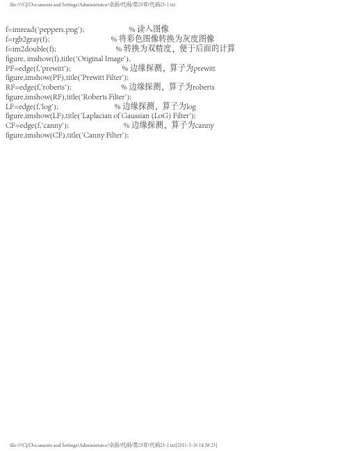
f=rgb2gray(f); % 将彩色图像转换为灰度图像f=im2double(f); % 转换为双精度，便于后面的计算figure, imshow(f),title('Original Image'),PF=edge(f,'prewitt'); % 边缘探测，算子为prewitt figure,imshow(PF),title('Prewitt Filter');RF=edge(f,'roberts'); % 边缘探测，算子为roberts figure,imshow(RF),title('Roberts Filter');LF=edge(f,'log'); % 边缘探测，算子为logfigure,imshow(LF),title('Laplacian of Gaussian (LoG) Filter');CF=edge(f,'canny'); % 边缘探测，算子为canny figure,imshow(CF),title('Canny Filter');f=rgb2gray(f); % 灰度转换f=im2double(f); % 数据类型转换% 使用垂直Sobel算子，自动选择阈值[VSFAT Threshold]=edge(f,'sobel','vertical'); % 边缘探测figure, imshow(f),title('Original Image'), % 显示原始图像figure,imshow(VSFAT),title('Sobel Filter - Automatic Threshold'); % 显示边缘探测图像%使用水平和垂直Sobel算子，自动选择阈值SFST=edge(f,'sobel',Threshold);figure,imshow(SFST),title('Sobel Filter (Horizontal and Vertical)'); % 显示边缘探测图像%使用指定45度角Sobel算子滤波器，指定阈值s45=[-2 -1 0;-1 0 1;0 1 2];SFST45=imfilter(f,s45,'replicate');SFST45=SFST45>=Threshold;figure,imshow(SFST45),title('Sobel Filter (45 Degree)'); % 显示边缘探测图像%使用指定-45度角Sobel算子滤波器，指定阈值sm45=[0 1 2;-1 0 1;-2 -1 0];SFSTM45=imfilter(f,sm45,'replicate');SFSTM45=SFSTM45>=Threshold;figure,imshow(SFSTM45),title('Sobel Filter (-45 Degree)'); % 显示边缘探测图像I = imread('circuit.tif');rotI = imrotate(I,33,'crop'); % 图像旋转，该函数具体用法在本书13.3.3有介绍。

图像分割代码

Canny边缘分割clc;a = imread('1.bmp');a=rgb2gray(a); % 选取的是jpg格式的图片，试用要进行灰度处理imshow(a);title('灰度图');ffta = fft2(a); % 获取2维离散傅里叶变化后的图像，保存到fftIsffta = fftshift(ffta); % 将傅里叶变化的中心移到图像中心，保存到sfftIRR = real(sffta); % 取实部II = imag(sffta); % 取虚部A = sqrt(RR.^2 + II.^2); % 计算频谱幅值A = (A - min(min(A)))/(max(max(A)) - min(min(A)))*225; % 灰度拉升，将变换后的图像拉升到0~255区间b=edge(a,'canny',[0.03,0.06]); %灰度图的边缘提取c=edge(a,'canny',[0.05,0.1]);d=edge(a,'canny',[0.05,0.1],2);figure;subplot(1,3,1),imshow(b), axis on;title('canny 阈值=0.02');subplot(1,3,2),imshow(c), axis on;title('canny 阈值=0.07');subplot(1,3,3),imshow(d),axis on;title('默认');figure;imshow(A);title('频谱图');Soble算子-阈值不同时的边缘分割a = imread('1.bmp');a=rgb2gray(a); % 灰度处理b=edge(a,'sobel',0.02);c=edge(a,'sobel',0.07);[d,e]=edge(a,'sobel');subplot(1,3,1),imshow(b), axis on;title('sobel 阈值=0.02');subplot(1,3,2),imshow(c), axis on;title('sobel 阈值=0.07')subplot(1,3,3),imshow(d),axis on;title('默认');四种算子的边缘分割I=imread('1.bmp');I=rgb2gray(I);imshow(I);title('原始图像');BW1=edge(I,'Roberts ',0.3); %edge调用Roberts为检测算子判别阈值为0.3 figure,imshow(BW1);title( '阈值为0.3的Roberts算子边缘检测图像');BW2=edge(I, 'sobel ',0.3); %edge调用sobel为检测算子判别阈值为0.3 figure,imshow(BW2);title( '阈值为0.3的sobel算子边缘检测图像');BW3=edge(I,'Prewitt ',0.3); %edge调用Prewitt为检测算子判别阈值为0.3 figure,imshow(BW3);title( '阈值为0.3的Prewitt算子边缘检测图像');BW4= edge(I,'Canny',0.3) ;%edge调用Canny为检测算子判别阈值为0.3 figure,imshow(BW4);title( '阈值为0.3的Canny算子边缘检测图像');A=BW1(x,y);B=BW2(x,y);C=BW3(x,y);D=BW4(x,y);E=A+B+C+D;figure,imshow(E);title( 'jia');LOG算子边缘分割I=imread ('1.bmp');I=rgb2gray(I);BW1=edge(I,'log',0.00);figure,imshow(BW1);title('阈值为0.00的LOG算子边缘检测图像');BW11=edge(I,'log',0.01);figure,imshow(BW11);title('阈值为0.01的LOG算子边缘检测图像');BW2= edge(I,'log',0.03);figure,imshow(BW2);title('阈值为0.03的LOG算子边缘检测图像');BW22= edge(I,'log',0.05);figure,imshow(BW22);title('阈值为0.05的LOG算子边缘检测图像');加噪后均值滤波clc;img=imread('1.bmp');img_0=rgb2gray(img);img_1=imnoise(img_0,'salt & pepper',0.02);img_2=medfilt2(img_1);subplot(2,2,1);imshow(img);title('原始图像');subplot(2,2,2);imshow(img_1);title('加入噪声后图像'); subplot(2,2,3);imshow(img_2);title('中值滤波后图像');加噪声后中值滤波clc;img=imread('1.bmp');img_0=rgb2gray(img);img_1=imnoise(img_0,'salt & pepper',0.02);img_2=medfilt2(img_1);subplot(2,2,1);imshow(img);title('原始图像');subplot(2,2,2);imshow(img_1);title('加入噪声后图像'); subplot(2,2,3);imshow(img_2);title('中值滤波后图像');阈值分割clc;A=imread('1.bmp');figuresubplot(1,5,1),imshow(A);title('原图像')B=im2bw(A,91/255);subplot(1,5,2),imshow(B);title('阈值91的图像')C=im2bw(A,71/255);subplot(1,5,3),imshow(C);title('阈值71的图像')双重处理A=imread('1.bmp');figure,B=rgb2gray(A);C=imnoise(B,'salt & pepper',0.02);D=medfilt2(B);subplot(2,2,1)imshow(A)title('原始图像')subplot(2,2,2)imshow(D)title('中值滤波')E=im2bw(D,91/255);subplot(2,2,3),imshow(E);title('阈值91的中值滤波图像'), F=im2bw(D,71/255);subplot(2,2,4),imshow(F);title('阈值71的中值滤波图像'),。

matlab regiongrowing函数源码

matlab regiongrowing函数源码引言概述：
Matlab是一种广泛应用于科学计算和工程领域的编程语言和开发环境。

其中，regiongrowing函数是Matlab中用于图像分割的重要函数之一。

本文将详细介绍regiongrowing函数的源码，并解释其实现原理和应用。

正文内容：
1. regiongrowing函数的功能
1.1 基本功能
1.2 扩展功能
2. regiongrowing函数的实现原理
2.1 区域生长算法
2.2 阈值选择策略
2.3 邻域定义
3. regiongrowing函数的应用
3.1 图像分割
3.2 特定区域提取
3.3 目标检测
4. regiongrowing函数的使用示例
4.1 函数调用
4.2 参数设置
4.3 结果展示
5. regiongrowing函数的优化方法
5.1 并行计算
5.2 邻域优化
5.3 阈值自适应
总结：
在本文中，我们详细介绍了Matlab中的regiongrowing函数的源码，包括其功能、实现原理、应用和优化方法。

regiongrowing函数在图像分割、特定区域提取和目标检测等领域具有广泛的应用。

通过合理设置参数和优化算法，可以提高函数的效率和准确性。

希望本文对读者理解和使用regiongrowing函数有所帮助。

数字图像处理代码Ch7《图像分割》

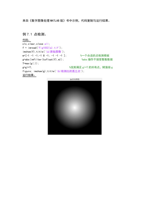
来自《数字图像处理MATLAB版》书中示例，代码复制与运行结果。

例7.1 点检测。

代码：clc,clear,close all;f = imread('Fig1002(a).tif');imshow(f),title('(a)原始图像');w=[-1 -1 -1;-1 8 -1; -1 -1 -1 ]; %一个合适的点检测模板g=abs(imfilter(tofloat(f),w)); %abs操作不接受整数数据T=max(g(:));g=g>=T; %找到满足g>=T的所有点，赋值给g figure; imshow(g);title('(b)检测出的孤立点');运行结果：例7.2 检测指定方向的线。

代码：clc;clear,close all;f = imread('Fig1004(a).tif');subplot 231; imshow(f);title('(a)连线模板图像')w = [2 -1 -1;-1 2 -1; -1 -1 2]; %+45度线检测模板g = imfilter(tofloat(f),w);subplot 232 ,imshow(g,[]),title('(b)使用 +45度检测器处理后的图像') gtop = g(1:150,1:150); %左上角部分gtop = pixeldup(gtop,4); %enlarge by pixel duplication(就是维度*4) subplot 233; imshow(gtop,[])title('(c)+45度检测器处理后的图像左上角') gbot = g(end-119:end,end-119:end);gbot = pixeldup(gbot,4);subplot 234 ;imshow(gbot,[]),title('(d)-45度检测器处理后的图像右下角') g = abs(g);subplot 235; imshow(g,[]),title('(e)图(b)的绝对值')T = max(g(:)); g = g>=T;subplot 236 ;imshow(g),title('(f)满足条件[g>=T]的所有点（白色点）[其中g是图(e)]')运行结果：例7.3 使用Sobel边缘检测器。

matlab二值化分割代码

matlab二值化分割代码
以下是一个简单的 MATLAB 代码示例，用于对图像进行二值化分割：
matlab.
% 读取图像。

img = imread('your_image.jpg');
% 将图像转换为灰度图像。

gray_img = rgb2gray(img);
% 使用Otsu方法进行图像二值化。

level = graythresh(gray_img);
bw_img = imbinarize(gray_img,level);
% 显示原始图像和二值化图像。

subplot(1,2,1), imshow(gray_img), title('Original Image');
subplot(1,2,2), imshow(bw_img), title('Binary Image');
在这个示例中，首先使用 `imread` 函数读取图像，然后使用`rgb2gray` 函数将图像转换为灰度图像。

接下来，使用
`graythresh` 函数确定阈值，并使用 `imbinarize` 函数将灰度图像转换为二值化图像。

最后，使用 `subplot` 和 `imshow` 函数显示原始图像和二值化图像。

需要注意的是，这只是一个简单的二值化分割示例。

实际应用中可能需要根据具体的图像特征和要求进行参数调整和算法优化。

数字图像处理图像分割代码

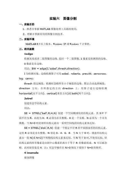
实验六图像分割一、实验目的1、熟悉并掌握MATLAB图像处理工具箱的使用；2、理解并掌握常用的图像分割技术。

二、实验环境MATLAB 6.5以上版本、Windows XP或Windows 7计算机。

三、相关函数1edge检测灰度或者二值图像的边缘，返回一个二值图像，1像素是检测到的边缘，0像素是非边缘。

用法：BW = edge(I,'sobel',thresh,direction)，I为检测对象；边缘检测算子可用sobel，roberts，prewitt，zerocross，log，canny；thresh指定阈值，检测时忽略所有小于阈值的边缘，默认自动选择阈值；direction方向，在所指定的方向direction上，用算子进行边缘检测horizontal(水平方向)、vertical(垂直方向)或both(两个方向)。

2strel创建形态学结构元素。

用法：SE = STREL('ball',R,H,N) 创建一个空间椭球状的结构元素，其X-Y平面半径为R，高度为H。

R必须为非负整数，H是一个实数。

N必须为一个非负偶数。

当N>0时此球形结构元素由一系列空间线段结构元素来近似。

SE = STREL('disk',R,N) 创建一个指定半径R的平面圆盘形的结构元素。

这里R必须是非负整数。

N须是0，4，6，8。

当N大于0时，圆盘形结构元素由一组N(或N+2)个周期线结构元素来近似。

当N等于0时,不使用近似，即结构元素的所有像素是由到中心像素距离小于等于R的像素组成。

N可以被忽略，此时缺省值是4。

注: 形态学操作在N>0情况下要快于N=0的情形。

4 imerode腐蚀图像用法：IM2 = imerode(IM,SE)腐蚀灰度、二进制或压缩二进制图像IM ，返回腐蚀图像IM2 。

参数SE 是函数strel 返回的一个结构元素体或是结构元素体阵列。

图像分割部分源代码

1.图像反转MATLAB程序实现如下：I=imread('xian.bmp');J=double(I);J=-J+(256-1); %图像反转线性变换H=uint8(J);subplot(1,2,1),imshow(I);subplot(1,2,2),imshow(H);2.灰度线性变换MATLAB程序实现如下：I=imread('xian.bmp');subplot(2,2,1),imshow(I);title('原始图像');axis([50,250,50,200]);axis on; %显示坐标系I1=rgb2gray(I);subplot(2,2,2),imshow(I1);title('灰度图像');axis([50,250,50,200]);axis on; %显示坐标系J=imadjust(I1,[0.1 0.5],[]); %局部拉伸，把[0.1 0.5]内的灰度拉伸为[0 1] subplot(2,2,3),imshow(J);title('线性变换图像[0.1 0.5]');axis([50,250,50,200]);grid on; %显示网格线axis on; %显示坐标系K=imadjust(I1,[0.3 0.7],[]); %局部拉伸，把[0.3 0.7]内的灰度拉伸为[0 1] subplot(2,2,4),imshow(K);title('线性变换图像[0.3 0.7]');axis([50,250,50,200]);grid on; %显示网格线axis on; %显示坐标系3.非线性变换MATLAB程序实现如下：I=imread('xian.bmp');I1=rgb2gray(I);subplot(1,2,1),imshow(I1);title('灰度图像');axis([50,250,50,200]);grid on; %显示网格线axis on; %显示坐标系J=double(I1);J=40*(log(J+1));H=uint8(J);subplot(1,2,2),imshow(H);title('对数变换图像');axis([50,250,50,200]);grid on; %显示网格线axis on; %显示坐标系4.直方图均衡化MATLAB程序实现如下：I=imread('xian.bmp');I=rgb2gray(I);figure;subplot(2,2,1);imshow(I);subplot(2,2,2);imhist(I);I1=histeq(I);figure;subplot(2,2,1);imshow(I1);subplot(2,2,2);imhist(I1);5.线性平滑滤波器用MATLAB实现领域平均法抑制噪声程序：I=imread('xian.bmp');subplot(231)imshow(I)title('原始图像')I=rgb2gray(I);I1=imnoise(I,'salt & pepper',0.02);subplot(232)imshow(I1)title('添加椒盐噪声的图像')k1=filter2(fspecial('average',3),I1)/255; %进行3*3模板平滑滤波k2=filter2(fspecial('average',5),I1)/255; %进行5*5模板平滑滤波k3=filter2(fspecial('average',7),I1)/255; %进行7*7模板平滑滤波k4=filter2(fspecial('average',9),I1)/255; %进行9*9模板平滑滤波subplot(233),imshow(k1);title('3*3模板平滑滤波');subplot(234),imshow(k2);title('5*5模板平滑滤波');subplot(235),imshow(k3);title('7*7模板平滑滤波');subplot(236),imshow(k4);title('9*9模板平滑滤波');6.中值滤波器用MATLAB实现中值滤波程序如下：I=imread('xian.bmp');I=rgb2gray(I);J=imnoise(I,'salt&pepper',0.02);subplot(231),imshow(I);title('原图像');subplot(232),imshow(J);title('添加椒盐噪声图像');k1=medfilt2(J); %进行3*3模板中值滤波k2=medfilt2(J,[5,5]); %进行5*5模板中值滤波k3=medfilt2(J,[7,7]); %进行7*7模板中值滤波k4=medfilt2(J,[9,9]); %进行9*9模板中值滤波subplot(233),imshow(k1);title('3*3模板中值滤波'); subplot(234),imshow(k2);title('5*5模板中值滤波'); subplot(235),imshow(k3);title('7*7模板中值滤波'); subplot(236),imshow(k4);title('9*9模板中值滤波');7.用Sobel算子和拉普拉斯对图像锐化：I=imread('xian.bmp');subplot(2,2,1),imshow(I);title('原始图像');axis([50,250,50,200]);grid on; %显示网格线axis on; %显示坐标系I1=im2bw(I);subplot(2,2,2),imshow(I1);title('二值图像');axis([50,250,50,200]);grid on; %显示网格线axis on; %显示坐标系H=fspecial('sobel'); %选择sobel算子J=filter2(H,I1); %卷积运算subplot(2,2,3),imshow(J);title('sobel算子锐化图像');axis([50,250,50,200]);grid on; %显示网格线axis on; %显示坐标系h=[0 1 0,1 -4 1,0 1 0]; %拉普拉斯算子J1=conv2(I1,h,'same'); %卷积运算subplot(2,2,4),imshow(J1);title('拉普拉斯算子锐化图像');axis([50,250,50,200]);grid on; %显示网格线axis on; %显示坐标系8.梯度算子检测边缘用MATLAB实现如下：I=imread('xian.bmp');subplot(2,3,1);imshow(I);title('原始图像');axis([50,250,50,200]);grid on; %显示网格线axis on; %显示坐标系I1=im2bw(I);subplot(2,3,2);imshow(I1);title('二值图像');axis([50,250,50,200]);grid on; %显示网格线axis on; %显示坐标系I2=edge(I1,'roberts');figure;subplot(2,3,3);imshow(I2);title('roberts算子分割结果');axis([50,250,50,200]);grid on; %显示网格线axis on; %显示坐标系I3=edge(I1,'sobel');subplot(2,3,4);imshow(I3);title('sobel算子分割结果');axis([50,250,50,200]);grid on; %显示网格线axis on; %显示坐标系I4=edge(I1,'Prewitt');subplot(2,3,5);imshow(I4);title('Prewitt算子分割结果');axis([50,250,50,200]);grid on; %显示网格线axis on; %显示坐标系9.LOG算子检测边缘用MATLAB程序实现如下：I=imread('xian.bmp');subplot(2,2,1);imshow(I);title('原始图像');I1=rgb2gray(I);subplot(2,2,2);imshow(I1);title('灰度图像');I2=edge(I1,'log');subplot(2,2,3);imshow(I2);title('log算子分割结果');10.Canny算子检测边缘用MATLAB程序实现如下：I=imread('xian.bmp');subplot(2,2,1);imshow(I);title('原始图像')I1=rgb2gray(I);subplot(2,2,2);imshow(I1);title('灰度图像');I2=edge(I1,'canny');subplot(2,2,3);imshow(I2);title('canny算子分割结果');11.边界跟踪（bwtraceboundary函数）clcclear allI=imread('xian.bmp');figureimshow(I);title('原始图像');I1=rgb2gray(I); %将彩色图像转化灰度图像threshold=graythresh(I1); %计算将灰度图像转化为二值图像所需的门限BW=im2bw(I1, threshold); %将灰度图像转化为二值图像figureimshow(BW);title('二值图像');dim=size(BW);col=round(dim(2)/2)-90; %计算起始点列坐标row=find(BW(:,col),1); %计算起始点行坐标connectivity=8;num_points=180;contour=bwtraceboundary(BW,[row,col],'N',connectivity,num_points);%提取边界figureimshow(I1);hold on;plot(contour(:,2),contour(:,1), 'g','LineWidth' ,2);title('边界跟踪图像');12.Hough变换I= imread('xian.bmp');rotI=rgb2gray(I);subplot(2,2,1);imshow(rotI);title('灰度图像');axis([50,250,50,200]);grid on;axis on;BW=edge(rotI,'prewitt');subplot(2,2,2);imshow(BW);title('prewitt算子边缘检测后图像');axis([50,250,50,200]);grid on;axis on;[H,T,R]=hough(BW);subplot(2,2,3);imshow(H,[],'XData',T,'YData',R,'InitialMagnification','fit'); title('霍夫变换图');xlabel('\theta'),ylabel('\rho');axis on , axis normal, hold on;P=houghpeaks(H,5,'threshold',ceil(0.3*max(H(:))));x=T(P(:,2));y=R(P(:,1));plot(x,y,'s','color','white');lines=houghlines(BW,T,R,P,'FillGap',5,'MinLength',7); subplot(2,2,4);,imshow(rotI);title('霍夫变换图像检测');axis([50,250,50,200]);grid on;axis on;hold on;max_len=0;for k=1:length(lines)xy=[lines(k).point1;lines(k).point2];plot(xy(:,1),xy(:,2),'LineWidth',2,'Color','green');plot(xy(1,1),xy(1,2),'x','LineWidth',2,'Color','yellow');plot(xy(2,1),xy(2,2),'x','LineWidth',2,'Color','red');len=norm(lines(k).point1-lines(k).point2);if(len>max_len)max_len=len;xy_long=xy;endendplot(xy_long(:,1),xy_long(:,2),'LineWidth',2,'Color','cyan');13.直方图阈值法用MATLAB实现直方图阈值法：I=imread('xian.bmp');I1=rgb2gray(I);figure;subplot(2,2,1);imshow(I1);title('灰度图像')axis([50,250,50,200]);grid on; %显示网格线axis on; %显示坐标系[m,n]=size(I1); %测量图像尺寸参数GP=zeros(1,256); %预创建存放灰度出现概率的向量for k=0:255GP(k+1)=length(find(I1==k))/(m*n); %计算每级灰度出现的概率，将其存入GP中相应位置endsubplot(2,2,2),bar(0:255,GP,'g') %绘制直方图title('灰度直方图')xlabel('灰度值')ylabel('出现概率')I2=im2bw(I,150/255);subplot(2,2,3),imshow(I2);title('阈值150的分割图像')axis([50,250,50,200]);grid on; %显示网格线axis on; %显示坐标系I3=im2bw(I,200/255); %subplot(2,2,4),imshow(I3);title('阈值200的分割图像')axis([50,250,50,200]);grid on; %显示网格线axis on; %显示坐标系14. 自动阈值法：Otsu法用MATLAB实现Otsu算法：clcclear allI=imread('xian.bmp');subplot(1,2,1),imshow(I);title('原始图像')axis([50,250,50,200]);grid on; %显示网格线axis on; %显示坐标系level=graythresh(I); %确定灰度阈值BW=im2bw(I,level);subplot(1,2,2),imshow(BW);title('Otsu法阈值分割图像')axis([50,250,50,200]);grid on; %显示网格线axis on; %显示坐标系15.膨胀操作I=imread('xian.bmp'); %载入图像I1=rgb2gray(I);subplot(1,2,1);imshow(I1);title('灰度图像')axis([50,250,50,200]);grid on; %显示网格线axis on; %显示坐标系se=strel('disk',1); %生成圆形结构元素I2=imdilate(I1,se); %用生成的结构元素对图像进行膨胀subplot(1,2,2);imshow(I2);title('膨胀后图像');axis([50,250,50,200]);grid on; %显示网格线axis on; %显示坐标系16.腐蚀操作MATLAB实现腐蚀操作I=imread('xian.bmp'); %载入图像I1=rgb2gray(I);subplot(1,2,1);imshow(I1);title('灰度图像')axis([50,250,50,200]);grid on; %显示网格线axis on; %显示坐标系se=strel('disk',1); %生成圆形结构元素I2=imerode(I1,se); %用生成的结构元素对图像进行腐蚀subplot(1,2,2);imshow(I2);title('腐蚀后图像');axis([50,250,50,200]);grid on; %显示网格线axis on; %显示坐标系17.开启和闭合操作用MATLAB实现开启和闭合操作I=imread('xian.bmp'); %载入图像subplot(2,2,1),imshow(I);title('原始图像');axis([50,250,50,200]);axis on; %显示坐标系I1=rgb2gray(I);subplot(2,2,2),imshow(I1);title('灰度图像');axis([50,250,50,200]);axis on; %显示坐标系se=strel('disk',1); %采用半径为1的圆作为结构元素I2=imopen(I1,se); %开启操作I3=imclose(I1,se); %闭合操作subplot(2,2,3),imshow(I2);title('开启运算后图像');axis([50,250,50,200]);axis on; %显示坐标系subplot(2,2,4),imshow(I3);title('闭合运算后图像');axis([50,250,50,200]);axis on; %显示坐标系18.开启和闭合组合操作I=imread('xian.bmp'); %载入图像subplot(3,2,1),imshow(I);title('原始图像');axis([50,250,50,200]);axis on; %显示坐标系I1=rgb2gray(I);subplot(3,2,2),imshow(I1);title('灰度图像');axis([50,250,50,200]);axis on; %显示坐标系se=strel('disk',1);I2=imopen(I1,se); %开启操作I3=imclose(I1,se); %闭合操作subplot(3,2,3),imshow(I2);title('开启运算后图像');axis([50,250,50,200]);axis on; %显示坐标系subplot(3,2,4),imshow(I3);title('闭合运算后图像');axis([50,250,50,200]);axis on; %显示坐标系se=strel('disk',1);I4=imopen(I1,se);I5=imclose(I4,se);subplot(3,2,5),imshow(I5); %开—闭运算图像title('开—闭运算图像');axis([50,250,50,200]);axis on; %显示坐标系I6=imclose(I1,se);I7=imopen(I6,se);subplot(3,2,6),imshow(I7); %闭—开运算图像title('闭—开运算图像');axis([50,250,50,200]);axis on; %显示坐标系19.形态学边界提取利用MATLAB实现如下：I=imread('xian.bmp'); %载入图像subplot(1,3,1),imshow(I);title('原始图像');axis([50,250,50,200]);grid on; %显示网格线axis on; %显示坐标系I1=im2bw(I);subplot(1,3,2),imshow(I1);title('二值化图像');axis([50,250,50,200]);grid on; %显示网格线axis on; %显示坐标系I2=bwperim(I1); %获取区域的周长subplot(1,3,3),imshow(I2);title('边界周长的二值图像');axis([50,250,50,200]);grid on;axis on;20.形态学骨架提取利用MATLAB实现如下：I=imread('xian.bmp'); subplot(2,2,1),imshow(I); title('原始图像');axis([50,250,50,200]); axis on;I1=im2bw(I);subplot(2,2,2),imshow(I1); title('二值图像');axis([50,250,50,200]); axis on;I2=bwmorph(I1,'skel',1); subplot(2,2,3),imshow(I2); title('1次骨架提取');axis([50,250,50,200]); axis on;I3=bwmorph(I1,'skel',2); subplot(2,2,4),imshow(I3); title('2次骨架提取');axis([50,250,50,200]); axis on;21.直接提取四个顶点坐标I = imread('xian.bmp');I = I(:,:,1);BW=im2bw(I);figureimshow(~BW)[x,y]=getpts。

MATLAB图像分割代码

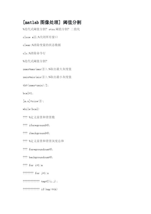
[matlab图像处理] 阈值分割%迭代式阈值分割? otsu阈值分割? 二值化close all;%关闭所有窗口clear;%清除变量的状态数据clc;%清除命令行%迭代式阈值分割?zmax=max(max(I));%取出最大灰度值zmin=min(min(I));%取出最小灰度值tk=(zmax+zmin)/2;bcal=1;[m,n]=size(I);while(bcal)??? %定义前景和背景数??? iforeground=0;??? ibackground=0;??? %定义前景和背景灰度总和??? foregroundsum=0;??? backgroundsum=0;??? for i=1:m??????? for j=1:n ??????????? tmp=I(i,j); ??????????? if(tmp>=tk)??????????????? %前景灰度值??????????????? iforeground=iforeground+1; ??????????????? foregroundsum=foregroundsum+double(tmp); ??????????? else??????????????? ibackground=ibackground+1; ??????????????? backgroundsum=backgroundsum+double(tmp); ??????????? end??????? end??? end??? %计算前景和背景的平均值??? z1=foregroundsum/iforeground;??? z2=foregroundsum/ibackground;??? tktmp=uint8((z1+z2)/2);??? if(tktmp==tk)??????? bcal=0;??? else??????? tk=tktmp;??? end??? %当阈值不再变化时,说明迭代结束enddisp(strcat('迭代的阈值:',num2str(tk)));%在command window里显示出 :迭代的阈值:阈值newI=im2bw(I,double(tk)/255);%函数im2bw使用阈值（threshold）变换法把灰度图像（grayscale image）???? %转换成二值图像。

FCM图像分割算法MATLAB源代码

FCM图像分割算法function fcmapp(file, cluster_n)% FCMAPP% fcmapp(file, cluter_n) segments a image named file using the algorithm% FCM.% [in]% file: the path of the image to be clustered.% cluster_n: the number of cluster for FCM.eval(['info=imfinfo(''',file, ''');']);switch info.ColorTypecase 'truecolor'eval(['RGB=imread(''',file, ''');']);% [X, map] = rgb2ind(RGB, 256);I = rgb2gray(RGB);clear RGB;case 'indexed'eval(['[X, map]=imread(''',file, ''');']);I = ind2gray(X, map);clear X;case 'grayscale'eval(['I=imread(''',file, ''');']);end;I = im2double(I);filename = file(1 : find(file=='.')-1);data = reshape(I, numel(I), 1);tic[center, U, obj_fcn]=fcm(data, cluster_n);elapsedtime = toc;%eval(['save(', filename, int2str(cluster_n),'.mat'', ''center'', ''U'', ''obj_fcn'', ''elapsedtime'');']); fprintf('elapsedtime = %d', elapsedtime);maxU=max(U);temp = sort(center, 'ascend');for n = 1:cluster_n;eval(['cluster',int2str(n), '_index = find(U(', int2str(n), ',:) == maxU);']);index = find(temp == center(n));switch indexcase 1color_class = 0;case cluster_ncolor_class = 255;otherwisecolor_class = fix(255*(index-1)/(cluster_n-1));endeval(['I(cluster',int2str(n), '_index(:))=', int2str(color_class),';']);end;filename = file(1:find(file=='.')-1);I = mat2gray(I);%eval(['imwrite(I,', filename,'_seg', int2str(cluster_n), '.bmp'');']);imwrite(I, 'temp\tu2_4.bmp','bmp');imview(I);function fcmapp(file, cluster_n)% FCMAPP% fcmapp(file, cluter_n) segments a image named file using the algorithm% FCM.% [in]% file: the path of the image to be clustered.% cluster_n: the number of cluster for FCM.eval(['info=imfinfo(''',file, ''');']);switch info.ColorTypecase 'truecolor'eval(['RGB=imread(''',file, ''');']);% [X, map] = rgb2ind(RGB, 256);I = rgb2gray(RGB);clear RGB;case 'indexed'eval(['[X, map]=imread(''',file, ''');']);I = ind2gray(X, map);clear X;case 'grayscale'eval(['I=imread(''',file, ''');']);end;I = im2double(I);filename = file(1 : find(file=='.')-1);data = reshape(I, numel(I), 1);tic[center, U, obj_fcn]=fcm(data, cluster_n);elapsedtime = toc;%eval(['save(', filename, int2str(cluster_n),'.mat'', ''center'', ''U'', ''obj_fcn'', ''elapsedtime'');']); fprintf('elapsedtime = %d', elapsedtime);maxU=max(U);temp = sort(center, 'ascend');for n = 1:cluster_n;eval(['cluster',int2str(n), '_index = find(U(', int2str(n), ',:) == maxU);']);index = find(temp == center(n));switch indexcase 1color_class = 0;case cluster_ncolor_class = 255;otherwisecolor_class = fix(255*(index-1)/(cluster_n-1));endeval(['I(cluster',int2str(n), '_index(:))=', int2str(color_class),';']); end;filename = file(1:find(file=='.')-1);I = mat2gray(I);%eval(['imwrite(I,', filename,'_seg', int2str(cluster_n), '.bmp'');']); imwrite(I, 'r.bmp');imview(I);主程序1ImageDir='.\';%directory containing the images%path('..') ;%cmpviapath('..') ;img=im2double(imresize(imread([ImageDir '12.png']),2)) ;figure(1) ; imagesc(img) ; axis image[ny,nx,nc]=size(img) ;imgc=applycform(img,makecform('srgb2lab')) ;d=reshape(imgc(:,:,2:3),ny*nx,2) ;d(:,1)=d(:,1)/max(d(:,1)) ; d(:,2)=d(:,2)/max(d(:,2)) ;%d=d ./ (repmat(sqrt(sum(d.^2,2)),1,3)+eps()) ;k=4 ; % number of clusters%[l0 c] = kmeans(d, k,'Display','iter','Maxiter',100);[l0 c] = kmeans(d, k,'Maxiter',100);l0=reshape(l0,ny,nx) ;figure(2) ; imagesc(l0) ; axis image ;%c=[ 0.37 0.37 0.37 ; 0.77 0.73 0.66 ; 0.64 0.77 0.41 ; 0.81 0.76 0.58 ; ...%0.85 0.81 0.73 ] ;%c=[0.99 0.76 0.15 ; 0.55 0.56 0.15 ] ;%c=[ 0.64 0.64 0.67 ; 0.27 0.45 0.14 ] ;%c=c ./ (repmat(sqrt(sum(c.^2,2)),1,3)+eps()) ;% Data termDc=zeros(ny,nx,k) ;for i=1:k,dif=d-repmat(c(i,:),ny*nx,1) ;Dc(:,:,i)= reshape(sum(dif.^2,2),ny,nx) ;end ;% Smoothness termSc=(ones(k)-eye(k)) ;% Edge termsg = fspecial('gauss', [13 13], 2);dy = fspecial('sobel');vf = conv2(g, dy, 'valid');Vc = zeros(ny,nx);Hc = Vc;for b=1:nc,Vc = max(Vc, abs(imfilter(img(:,:,b), vf, 'symmetric')));Hc = max(Hc, abs(imfilter(img(:,:,b), vf', 'symmetric'))); endgch=char;gch = GraphCut('open', 1*Dc, Sc,exp(-5*Vc),exp(-5*Hc)); [gch l] = GraphCut('expand',gch);gch = GraphCut('close', gch);label=l(100,200) ;lb=(l==label) ;lb=imdilate(lb,strel('disk',1))-lb ;figure(3) ; image(img) ; axis image ; hold on ;contour(lb,[1 1],'r') ; hold off ; title('no edges') ;figure(4) ; imagesc(l) ; axis image ; title('no edges') ;gch = GraphCut('open', Dc, 5*Sc,exp(-10*Vc),exp(-10*Hc)); [gch l] = GraphCut('expand',gch);gch = GraphCut('close', gch);lb=(l==label) ;lb=imdilate(lb,strel('disk',1))-lb ;figure(5) ; image(img) ; axis image ; hold on ;contour(lb,[1 1],'r') ; hold off ; title('edges') ;figure(6) ; imagesc(l) ; axis image ; title('edges') ;主程序2I = imread( '12.png' );I = rgb2gray(I);subplot(5,3,1),imshow(I);k=medfilt2(I,[5,5]);subplot(5,3,2),imshow(k);title('5*5中值滤波图像');%f=imread('tuxiang1.tif');%subplot(1,2,1),imshow(f);%title('原图像');g1=histeq(k,256);subplot(5,3,3),imshow(g1);title('直方图匹配');%g2=histeq(k2,256);%subplot(2,2,2),imshow(g2);%title('5*5直方图匹配');%k=medfilt2(f,[5,5]);%k2=medfilt2(f,[5,5]);%j=imnoise(f,'gaussian',0,0.005);%subplot(1,3,3),imshow(k2);%title('5*5中值滤波图像');hy = fspecial( 'sobel' );hx = hy;Iy = imfilter(double(g1), hy, 'replicate' );Ix = imfilter(double(g1), hx, 'replicate' );gradmag = sqrt(Ix.^2 + Iy.^2);subplot(5,3,4), imshow(gradmag,[ ]), title( 'gradmag' );L = watershed(gradmag);Lrgb = label2rgb(L);subplot(5,3,5), imshow(Lrgb), title( 'Lrgb' );se = strel( 'disk' , 9);Io = imopen(g1, se);subplot(5,3,6), imshow(Io), title( 'Io' )Ie = imerode(g1, se);Iobr = imreconstruct(Ie, g1);subplot(5,3,7), imshow(Iobr), title( 'Iobr' );Ioc = imclose(Io, se);subplot(5,3,8), imshow(Ioc), title( 'Ioc' );Iobrd = imdilate(Iobr, se);Iobrcbr = imreconstruct(imcomplement(Iobrd), imcomplement(Iobr)); Iobrcbr = imcomplement(Iobrcbr);subplot(5,3,9), imshow(Iobrcbr), title( 'Iobrcbr' );fgm = imregionalmax(Iobrcbr);subplot(5,3,10), imshow(fgm), title( 'fgm' );I2 = g1; I2(fgm) = 255;subplot(5,3,11),imshow(I2), title( 'fgm superimposed on original image' );se2 = strel(ones(5,5)); I3 = g1; I3(fgm) = 255;subplot(5,3,12) ,imshow(I3);title( 'fgm4 superimposed on original image' );bw = im2bw(Iobrcbr, graythresh(Iobrcbr));subplot(5,3,13) , imshow(bw), title( 'bw' );D = bwdist(bw); DL = watershed(D);bgm = DL == 0;subplot(5,3,14) , imshow(bgm), title( 'bgm' );gradmag2 = imimposemin(gradmag, bgm | fgm);L = watershed(gradmag2);I4 = g1;I4(imdilate(L == 0, ones(3, 3)) | bgm | fgm) = 255;figure, imshow(I4);title( 'Markers and object boundaries superimposed on original image' ); Lrgb = label2rgb(L, 'jet' , 'w' , 'shuffle' );figure, imshow(Lrgb);title( 'Lrgb' );figure, imshow(I), hold onhimage = imshow(Lrgb);set(himage, 'AlphaData' , 0.3);title( 'Lrgb superimposed transparently on original image' );。

matlab分水岭分割算法代码

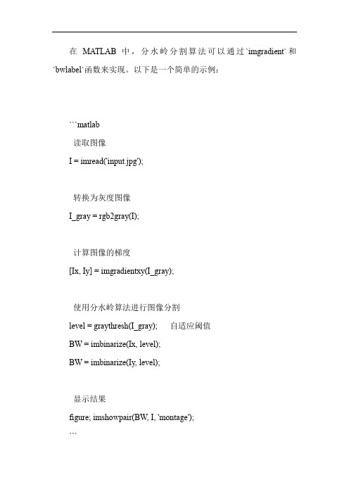
在MATLAB中，分水岭分割算法可以通过`imgradient`和`bwlabel`函数来实现。

以下是一个简单的示例：
```matlab
读取图像
I = imread('input.jpg');
转换为灰度图像
I_gray = rgb2gray(I);
计算图像的梯度
[Ix, Iy] = imgradientxy(I_gray);
使用分水岭算法进行图像分割
level = graythresh(I_gray); 自适应阈值
BW = imbinarize(Ix, level);
BW = imbinarize(Iy, level);
显示结果
figure; imshowpair(BW, I, 'montage');
```
以上代码首先读取一个图像，然后将其转换为灰度图像。

然后，计算图像的梯度。

最后，使用分水岭算法进行图像分割。

`graythresh`函数用于计算自适应阈值，`imbinarize`函数用于根据阈值将图像二值化。

最后，使用`imshowpair`函数来比较原始图像和分割后的图像。

需要注意的是，以上代码非常基础，可能无法处理复杂的图像分割任务。

对于更复杂的情况，可能需要更复杂的预处理步骤，例如去噪、区域增长等。

1、下载文档前请自行甄别文档内容的完整性，平台不提供额外的编辑、内容补充、找答案等附加服务。
2、"仅部分预览"的文档,不可在线预览部分如存在完整性等问题,可反馈申请退款(可完整预览的文档不适用该条件!)。
3、如文档侵犯您的权益，请联系客服反馈,我们会尽快为您处理(人工客服工作时间：9:00-18:30)。

subplot(2,2,2),imshow(I1);
title('灰度图像');
axis([50,250,50,200]);
axis on; %显示坐标系
J=imadjust(I1,[0.1 0.5],[]); %局部拉伸，把[0.1 0.5]内的灰度拉伸为[0 1]
I4=edge(I1,'Prewitt');
subplot(2,3,5);
imshow(I4);
title('Prewitt算子分割结果');
axis([50,250,50,200]);
grid on; %显示网格线
axis on; %显示坐标系
1.图像反转
MATLAB程序实现如下：
I=imread('xian.bmp');
J=double(I);
J=-J+(256-1); %图像反转线性变换
H=uint8(J);
subplot(1,2,1),imshow(I);
subplot(1,2,2),imshow(H);
I2=edge(I1,'log');
subplot(2,2,3);
imshow(I2);
title('log算子分割结果');
10.Canny算子检测边缘
用MATLAB程序实现如下：
I=imread('xian.bmp');
subplot(2,2,1);
imshow(I);
title('原始图像')
axis on; %显示坐标系
J=double(I1);
J=40*(log(J+1));
H=uint8(J);
subplot(1,2,2),imshow(H);
title('对数变换图像');
axis([50,250,50,200]);
grid on; %显示网格线
connectivity=8;
num_points=180;
contour=bwtraceboundary(BW,[row,col],'N',connectivity,num_points);
%提取边界
figure
imshow(I1);
subplot(233),imshow(k1);title('3*3模板平滑滤波');
subplot(234),imshow(k2);title('5*5模板平滑滤波');
subplot(235),imshow(k3);title('7*7模板平滑滤波');
subplot(236),imshow(k4);title('9*9模板平滑滤波');
7.用Sobel算子和拉普拉斯对图像锐化：
I=imread('xian.bmp');
subplot(2,2,1),imshow(I);
title('原始图像');
axis([50,250,50,200]);
grid on; %显示网格线
axis on; %显示坐标系
axis on; %显序实现如下：
I=imread('xian.bmp');
I=rgb2gray(I);
figure;
subplot(2,2,1);
imshow(I);
subplot(2,2,2);
imhist(I);
h=[0 1 0,1 -4 1,0 1 0]; %拉普拉斯算子
J1=conv2(I1,h,'same'); %卷积运算
subplot(2,2,4),imshow(J1);
title('拉普拉斯算子锐化图像');
axis([50,250,50,200]);
grid on; %显示网格线
title('原始图像')
I=rgb2gray(I);
I1=imnoise(I,'salt & pepper',0.02);
subplot(232)
imshow(I1)
title('添加椒盐噪声的图像')
k1=filter2(fspecial('average',3),I1)/255; %进行3*3模板平滑滤波
2.灰度线性变换
MATLAB程序实现如下：
I=imread('xian.bmp');
subplot(2,2,1),imshow(I);
title('原始图像');
axis([50,250,50,200]);
axis on; %显示坐标系
I1=rgb2gray(I);
I2=edge(I1,'roberts');
figure;
subplot(2,3,3);
imshow(I2);
title('roberts算子分割结果');
axis([50,250,50,200]);
grid on; %显示网格线
axis on; %显示坐标系
axis on; %显示坐标系
I1=im2bw(I);
subplot(2,3,2);
imshow(I1);
title('二值图像');
axis([50,250,50,200]);
grid on; %显示网格线
axis on; %显示坐标系
k2=filter2(fspecial('average',5),I1)/255; %进行5*5模板平滑滤波k3=filter2(fspecial('average',7),I1)/255; %进行7*7模板平滑滤波
k4=filter2(fspecial('average',9),I1)/255; %进行9*9模板平滑滤波
BW=im2bw(I1, threshold); %将灰度图像转化为二值图像
figure
imshow(BW);
title('二值图像');
dim=size(BW);
col=round(dim(2)/2)-90; %计算起始点列坐标
row=find(BW(:,col),1); %计算起始点行坐标
6.中值滤波器
用MATLAB实现中值滤波程序如下：
I=imread('xian.bmp');
I=rgb2gray(I);
J=imnoise(I,'salt&pepper',0.02);
subplot(231),imshow(I);title('原图像');
subplot(232),imshow(J);title('添加椒盐噪声图像');
I1=histeq(I);
figure;
subplot(2,2,1);
imshow(I1);
subplot(2,2,2);
imhist(I1);
5.线性平滑滤波器
用MATLAB实现领域平均法抑制噪声程序：
I=imread('xian.bmp');
subplot(231)
imshow(I)
axis on; %显示坐标系
8.梯度算子检测边缘
用MATLAB实现如下：
I=imread('xian.bmp');
subplot(2,3,1);
imshow(I);
title('原始图像');
axis([50,250,50,200]);
grid on; %显示网格线
9.LOG算子检测边缘
用MATLAB程序实现如下：
I=imread('xian.bmp');
subplot(2,2,1);
imshow(I);
title('原始图像');
I1=rgb2gray(I);
subplot(2,2,2);
imshow(I1);
title('灰度图像');
k1=medfilt2(J); %进行3*3模板中值滤波
k2=medfilt2(J,[5,5]); %进行5*5模板中值滤波
k3=medfilt2(J,[7,7]); %进行7*7模板中值滤波
k4=medfilt2(J,[9,9]); %进行9*9模板中值滤波
I1=rgb2gray(I);
subplot(2,2,2);
imshow(I1);
title('灰度图像');
I2=edge(I1,'canny');
subplot(2,2,3);
imshow(I2);
title('canny算子分割结果');
11.边界跟踪（bwtraceboundary函数）
subplot(233),imshow(k1);title('3*3模板中值滤波');
subplot(234),imshow(k2);title('5*5模板中值滤波');
subplot(235),imshow(k3);title('7*7模板中值滤波');