美国大学生数学建模2008年A题论文
2008年数学建模A题全国一等奖论文

2008年全国大学生数学建模竞赛A题全国一等奖论文数码相机定位摘要本文通过对数码相机的靶标和像平面相互之间关系的分析,利用选取相关对应点和坐标转换的方法,确定靶标圆心在像平面的投影位置,进而完成了系统标定模型,解决了相机的单目定位问题。
对于问题1,为确定靶标上圆的圆心在一个相机像平面的像坐标,需要得到相机像平面中点与靶标上点的对应关系。
通过将相机外部参数和内部参数联立可以建立模型1。
对于问题2,内部参数通过焦距可以得到,而外部参数的获得则需要事先确定一组特殊点。
由于靶标上两条线的交点在像平面上的投影点即为这两条线在像平面上的投影图线的交点,因此我们首先对图像进行边缘提取和椭圆拟合,然后利用程序选择靶标上A 、C 两个圆的外公共切线的切点作为特殊点。
将对应特殊点带入(1)式,就可以求得外部参数。
最后利用几何关系得出靶标上圆心的坐标,带入得到它们在该相机像平面的坐标。
结果为:vA O (-4.4324,-6.7785,0)、vB O (-2.3,-6.4456,0)、vC O (3.39,-5.9757,0)、vD O (-4.5471,3.7096,0)、vE O (2.1965,3.2275,0)。
见图3。
对于问题3,为了检验模型,本文通过计算机模拟数据,可以得到一个内外参数都已知的图像。
进而可以确定这四个顶点在像平面的准确坐标。
根据(1)式可以得到这四个顶点的计算坐标,把计算坐标与准确坐标的距离为对角线的矩形面积称为误差面积,误差率=误差面积/相纸面积。
计算误差率分别为:0.017591%、0.01777%、0.01532%、0.01557%。
从而可知用此模型精确度高,稳定性强。
对于问题4,类似于问题3,进行计算机模拟,得到空间两不同角度拍摄图像,进而得到在此数码相机坐标系下的特殊点坐标。
由于在求像坐标时考虑到了数码相机的透视效应,也就是内部参数,而两个数码相机的空间位置关系仅仅是外部参数的关系,因此可以求得仅考虑外部参数时两个像平面上的坐标,进而做差求出两个数码相机的相对位置坐标。
08年全国大学生数学建模A题 文档

R 旋转矩阵t 平移矢量K 相机标定矩阵AB(粗体)向量AB,粗体表示向量3尺寸、形状等信息,我们就可以确定靶标在三维空间中与相机的位置关系。
确定了靶标与相机的位置关系后,就可以很容易的将靶标上的点投射到靶标像平面上,当然也包括五个圆心。
在求取出五个圆心的空间坐标之后,将其投射到像平面上,就得到了第一问需要求的坐标。
在求解时涉及到一个问题,就是像平面上怎样确定切线。
因为像平面上的图形是不规则的,所以很难确定这些形状的切线。
因此我们考虑另外的方法,使用搜索的办法,利用模拟退火算法求解。
在如何检验模型的问题上,需要分两方面进行检验,一是精度,而是稳定性。
按照以上的方法求圆心在像平面上的坐标,并没有充分利用像平面上所有轮廓点的信息,因此可以利用这些点来检验模型的精度。
对于稳定性问题,可以采用计算机模拟的方法,随机修改图形的轮廓,并用以上的方法再次进行求解,通过比较修改前后的结果来分析模型的稳定性。
最后,考虑另外一台相机的定位相对位置问题。
根据前面模型,我们应能够对任意一台相机确定靶标相对它的位置,因此可以以这个靶标作为参照物,建立一个世界坐标系,将这两台相机的位置在这个坐标系里面表示出来,以此确定两台相机的相对位置。
四、模型假设1、假设靶标像的中心恰好在光轴上2、假设数码相机中图像平面与光轴垂直3、假设相机两个方向上焦距相等4、假设透镜的焦距很小,像距约等于焦距五、模型准备(一)靶图像矩阵表示首先将题目中的图片保存出来,得到的图像可以很方便的放到Matlab 里面进行处理。
但在处理之前还要进行进一步加工:(1) 将文件读入Matlab,使用imread()函数(2) 将矩阵变为0-1 矩阵对于用以上方式得到的矩阵,有两个值:0、15。
其中0 代表像素为白色的点,15代表像素为黑色的点。
为了方便下面处理,对需要把以上像素为15 的点值全部变为1。
以上两步的源代码见附录一。
4(二)图像轮廓的提取在提取图像轮廓时,首先要引入计算机图像处理技术中四邻域的概念。
2008年数学建模A题_数码相机定位【一等奖】

具有仿射不变性的几何结构在相机定位中的应用摘要本文采用小孔成像的模型研究相机成像问题。
基于靶平面上的点与像平面上的点一一对应,本文研究了几种几何结构。
发现靶平面上两个圆的内公切线交点与两个圆心共线这种几何结构仿射到像平面上依然成立,即两个圆心和内公切线交点在像平面上的3个像点共线,并证明了这一结论。
本文提出一种运用0-1矩阵求公切线的算法,但在实际操作时采用作图法。
运用作图法可以在像平面上确定两个椭圆的内公切线交点,该交点为靶平面上两个圆的内公切线交点在像平面上所成的像。
靶平面上5个圆可以确定10个内公切线交点,这样用作图法就可以确定靶平面上10个内公切线交点在像平面上的10个像点。
在像平面上建立坐标,每个靶平面上的圆心的像用两个未知量表示,共有10个未知量。
根据已证明的结论可知,对于每个内公切线交点在像平面上的像点,都有相对应的两个圆心的像点与之共线,就可以得到共线所满足的方程。
10个内公切线交点的像点对应10个2次方程,10个未知量就可求出。
靶平面上的圆心的像就可以确定。
本文采用牛顿迭代法对2次方程组进行求解。
并研究了解的稳定性。
为了得到两部固定相机的相对位置,建立了2个像平面坐标系、2个相机坐标系和1个三维世界坐标系。
本文采用最小二乘法确定相机坐标系与三维世界坐标系的关系。
在具体算法中,并没有利用所求出来的靶平面上圆心以及它的像点的坐标求解,而是采用10个内公切线交点及其像点的坐标求解,这是因为圆心的像点是由内公切线交点的像点求出的,误差更大。
分别确定2个相机坐标系与三维世界坐标系的关系之后,就可以确定2个相机坐标系之间的关系。
最后,本文对模型进行了分析,对一些方法的精度进行了讨论。
关键词相机定位仿射不变性内公切线交点1 问题分析双目定位是用两部相机给物体拍照来定位。
对于物体上的一个特征点,用两部不同位置的照相机拍照,就获得该点在两个像平面上的坐标。
如果知道两部相机的相对位置,就可以知道该特征点的具体位置。
(完整版)数模美赛08年A题

AbstractThe global temperature is rising rapidly today which has caused an extensive ice melt, so the study of predicting rising sea level because of ice melt in North Polar is essential. Our study will try to predict the impact to Florida from melting ice in North Polar .Our studies have three steps:●Predict the temperature: We did the prediction by Neural network and give thechange of temperature in 50 years, based on a large amount of data from the Intergovernmental Panel on Climate Change (IPCC);●Model the mass of ice melting and the sea level: The sea level model is mainlybased on the principle of Thermodynamics and iteration. The results demonstrate that the sea level will rise by 10.8 cm totally in 50 years. Prediction of our model can be proved to be credible by consulting the data from IPCC. We introduce a correct term αto modify our model. We can change αto simulate sea level rise in different temperature condition.●Analyze the impacts to Florida: We model the erosion of Florida’s shoreline tomake it clear that when sea level rise to a certain extent that Florida will face many serious problems such as flooding, destruction of biodiversity, (Health Care), Loss of agriculture production (salinization of soil) and so on over the next50 years.. We find the 17 cities or areas and 15 airports which are severelyimpacted by the rise of sea level.(Based on our results,) Without attaching more importance to solving the problem, shoreline of several coastal cities like Miami will be eroded seriously, and the lowest place−Key West will be disappeared. It will cost a huge financial loss, so further protection should be put into place.Content Introduction (3)Background (3)Our work (3)Study object: Ice cap in Greenland (3)Modeling the sea level (3)Analysis of Florida (3)Assumption (4)Model Ⅰ:Temperature Prediction (4)Grey Prediction Model: (4)Neural Network prediction Model: (4)Model Ⅱ:Melting ice and the rise of sea level (5)Model the rise of sea level (5)Heat from rise of temperature: (5)Mass of melting ice: (6)Design of Algorithms: (7)Model Results: Sea level will elevate by 10 centimeters in 50 years (7)Validation of our model: (8)Model ⅢAnalysis: The effects towards Florida (10)Major Cities Analysis (11)Miami (11)Tampa (11)Cape Coral (12)Key West (12)Other Impacts in Florida: (12)Recommendations to coastal Florida: (13)Judgments (13)Strengths (13)Weaknesses (13)Reference (14)IntroductionBackgroundGlobal Warming and sea level rise“Air temperatures at the top of the world continue to rise twice as fast as temperatures in lower latitudes, causing significant ice melt on land and sea” [Fears, December 17, 2014]. One of the serious consequences is that sea level will rise. Global average sea-level rose at an average rate of about 3.1[2.4 to 3.8] mm per year from 1993 to 2003[IPCC]. This information suggests that from 1993 to 2003 the sea-level rise by 3.1cm totally.Our workThe question requires us to predict the next 50 years’ condition of ice melting and analyze the effects on the Florida, especially some big cities. So we can separate this question into two parts:●How much and how fast will the see level rise within 50 years?●What are the effects on the Florida because of the rise of sea level, especiallysome big cities?Study object: Ice cap in GreenlandArctic mainly consists of Greenland, which occupies about 9% glaciers all over the world. Melting in Arctic is mainly due to Greenland, melting of floating ice can be ignored. So we can consider Greenland as study object.Modeling the sea levelWe develop a model for sea-level rise as the function of time. This model can predict sea-level rise in future.Analysis of FloridaAfter having calculated the increased sea level within next 50 years, we analyze the impact to the Florida.●Rising sea level can seriously threaten the development of cities. It has beenthreatening some islands and coastal cities. Over the next 18 years, about twothirds among 544 American towns will be twice as likely to face floods [Huang].More frequency hurricane will happen.●Sea water will corrode seacoast.● A large quantity of drinking water will be polluted.Assumption●Sea level rise is primarily due to the melting of ice cap in Green Land. We ignorethe other floating ice in the Northern Polar.●The increment of sea water from melting will flow over the oceans uniformly●Salt in the ice will not affects the procedure of melting.Model Ⅰ:Temperature PredictionGrey Prediction Model:The weakness of the grey prediction is that the result is increasing all the time. In other words, it cannot show the changes in detail.Neural Network prediction Model:Model Ⅱ:Melting ice and the rise of sea level Model the rise of sea levelThe main reason of the sea level rising is the melting of ice cap and the mass of melting ice is equal to the mass of sea water generated from melting. So, based on several physical principles, we model the rise of sea level by calculating the mass of melting ice. We assume that the increment of sea water from melting will flow over the world uniformly, which means the melting ice will contribute to the rise of sea level, divided by the area of the ocean.ρw V w=ρi V i=m i∆x=V w S oV w The increment of sea water from melting iceV i The total volume of melting ice capV m The total volume of water generated from melting∆x The sea level riseS o The overall ocean area: 361745300km2, this is 71 percent of earth’s total surface area (Wikipedia).Heat from rise of temperature:According to the principle of thermal transmission, heat will always be transmitted from high temperature to low temperature. So, the final state of stuff in the thermalcycling system will reach to a same temperature. So, we assume that the temperature of the whole ice cap will increase by ∆T when the world temperature rise by ∆T. However, it takes time for the ice cap to transmit the heat from the rise temperature. We use the ∆T every month to calculate the increase of melting ice in each month and get the total increment by accumulation, which means parts of the heat from temperature will be absorbed and used to melt ice. So, defining a coefficient(α)and we will have the heat which ice cap absorbs from the rising temperature in the n-th month:Q n=αc i(m c−∆m i(n−1))∆T nQ n The heat comes from rises of temperature in the n-th monthαThe coefficient of capacity of absorbing heat in one monthc i The specific heat capacity of icem c The mass of the whole ice cap 2.45×10¹⁶kg∆m in The mass of melting ice in the n-th month∆T n The change of temperature in the n-th monthWe try to find the α by calculating the mass of melting ice in known years. “Recently reported GrIS mass balance varies from near-balance to modest mass losses [47 to 97 gigatons (Gt) year−1] in the 1990s, increasing to a mass loss of 267 ± 38 Gt year−1 in 2007”(Michiel).α= 5.6735×10⁻³Mass of melting ice:The mass of melting ice in this month will depends on not only the rising temperature, but also the mass of melting ice in the last month.We divide the heat absorbed by the ice by the melting enthalpy of fusion for water to obtain the mass of extra melting ice resulted from the rise of temperature in this month.∆m in=∆m i(n−1)+Q n△fusHθmm i(k)=∑∆m in12kn=1∆m in The mass of melting ice in the n-th month△fusHθm: The melting enthalpy3.36×105J/kgm i(k)The total mass of melting ice in the next k yearsMoreover, “Since 2006, high summer melt rates have increased Greenland ice sheet mass loss to 273 gigatons per year” (Partitioning Recent Mass Loss). And the initial mass of melting ice in the first month will be calculated as follows:2.73×10¹⁴kg/12∆m i(−1)=m ii=2.73×101412kg∆x(k)=V wS o=m i(k)ρw S om ii: The mass of melting ice in the initial year.∆x(k)The total rise of sea level in the next k yearsDesign of Algorithms:Since we have the function ∆m in=f(∆m i(n−1),∆T n), we are able to calculate the mass of melting ice in the next n months using computer program with the data of temperatures and the initial amount of melting ice in the first month.This is easy to achieve using two linear arrays ∆m i[]and ∆T[]in MATLAB. Run a simple for loop from 2 to n and calculate ∆m in during each pass so that the whole ∆m i[]array can be found.So that the total amount of melting ice at n-th month is the summation from ∆m i[1] to ∆m i[n]. Also the total rise of sea level can be easily found.Model Results: Sea level will elevate by 10 centimeters in 50 years The solutions were coded using matlab:Figure 1: The mass of melting ice in the next 50 yearsFigure 2: The rise of sea level in the next 50 years The prediction about rise of sea level every decade in next 50 years:∆x(10)=0.9874 cm∆x(20)=2.5125 cm∆x(30)=4.6222 cm∆x(40)=7.3674 cm∆x(50)= 10.8037 cm Validation of our model:The results show that the sea level will elevate by approximately 10 centimeters totally and 2 millimeters/yr, which accord with the prediction in Relative Mean Sea Level trends from NOAA.Moreover, if we calculated the rise of sea level without considering the increase of temperature, which means sea level rise at the rate today in the next 50 years, the order of magnitudes is match up with our result. So, based on the analysis above, the results of our modelModel ⅢAnalysis: The effects towards FloridaBased on our results, the sea level will rise 10 centimeters in the following 50 years, which threaten Florida in the future and result in tremendous impacts. “Some 2.4 million people and 1.3 million homes, nearly half the risk nationwide, sit within 4 feet of the local high tide line. Sea level rise is more than doubling the risk of a storm surge at this level in South Florida.” (Florida and rising sea)Figure 3 the altitudes of Florida ()As we can see from this picture, most cities or counties in the southern Florida lie besides the coast. Statistic suggests that 17 counties with altitudes smaller than 3 feet will be threatened by the rise of sea level in 50 years. The counties and airports which will be involved are listed as follows:Cities: Miami, Homestead, Fort Lauderdale, West Palm Beach, Titusville, St Augustine, Clearwater, St Petersburg, Tampa, Brandon, Bradenton, Port Charlotte,Cape Coral, Bonita Springs, Naples, Marco Island, and Grand Isle.Airports: Miami International Airport, Fort Lauderdale International Airport, Central Florida Regional Airport, Cedar Knoll Flying Ranch, Daytona Beach Regional Airport, Craig Municipal Airport, Jacksonville International Airport, St George Island Airport.Major Cities AnalysisWe choose 4 metropolises which will be severely impacted to do some further analysis.MiamiMiami is the biggest city in Florida with the average elevation of 3 feet (0.9144m) [11ikipedia]. Also, it is a coastal city. So according to what we predict that sea level will rise 10.8037cm within 50 years, we can draw a conclusion that this city would be greatly influenced.The possibility of flooding would grow while the frequency of hurricane will increase. It is a big challenge to sewer system of Miami. According to our simulation, sea level rising would also threaten Miami International Airport. Another problem is that the sea water would gnaw at the shoreline. Many coastal man-made buildings are too closed to the sea which they would face a serious problem of being eroded. Aside from threatening of losing habitat, local drinking water would be polluted.TampaTampa is a city located on the west coast of Florida. It is the third largest city in Florida. It is famous because of tourism. Although the highest point in the city is only 48 feet (15 m) [wikipedia], rising sea level will do harm to its natural disaster. Tampais special because it has the Old Tampa Bay and Hillsborough Bay which is easy to be attacked by storm surge. Sea level rising would produce much more violent storm surge. The boundary of Tampa would also be lost. What’s more,Traffic facilities such as Tampa International Airport were under threatening of disappearing.Cape CoralThis city is famous because of its far-stretching beach and animated quay. Besides, it has more than 30 gardens and golf courses which attract many tourists. A variety of animals also promotes this city’s tourism. However, sea level rising would erode shoreline of Cape Coral. It would destroy natural environment of this area, and then damages biodiversity. And still worse, Pine Island would mostly disappear. So, the economic damage there will be hardly assessed.Key WestIt is an island of Florida, which have the lowest altitude. So if sea level rises to some extent, it would be the first to be under water.Other Impacts in Florida:Biodiversity: Wild life and rare animals in Florida will be impacted by loss of habitat and food. Moreover, it is hard for plants and animals in Florida to adapt the new climatic conditions and the increase of relative air humidity.Architecture:Sea level rise will cause salinization, which will impact the architectural production.Economy Pressure:More money will be put into the drainage systems and dam project, which means less city construction and business development.Health Care: Higher sea level will increase the risk of some disease like malaria.Recommendations to coastal Florida:●Build higher dams: In this way can cities hold back the rising flood waters.●Prepare for flooding: Complete supervisory control system. Guarantee thatcitizen can be evacuated in time.●Reduce carbon emission: More carbon emission means higher temperature, andthen lead to rising of sea level. So encourage citizen to live a low-carbon life.●Warn local citizen: Propagate relative knowledge of sea level rising to improvecitizen’s sense of self-protection when facing natural disaster. JudgmentsStrengths●We use Neural Network to predict temperature in future with a large amount ofreliable data. So our prediction of temperature in future is accurate relatively.●Our model can predict the sea level rising in different conditions, such asdifferent temperature.●Our model is relatively simple so it will take a little time to simulate. We caneasily get the result.Weaknesses●We ignore the areal variation about depth, salinity and temperature of the sea forsimplifying the model;●We neglect the floating ice which will bring some error;●We neglect the thermal expansion;The mode is only the function of time, so it can’t simulate unusual situations.ReferenceBen Strauss,Florida and rising sea,/news/floria-and-the-rising-seaFears, Darryl, Huang, Ming. “Rising sea level threatens millions of American and causes huge economic loss”. Souhu, March 16, 2012, 09:48 AM. Web. IPCC, http://www.ipcc.chMichiel van den Broeke,Partitioning Recent Mass Loss, Science 13 November 2009 “National Snow and Ice Data Center”, January 7, 2015。
美赛数学建模A题翻译版论文

美赛数学建模A题翻译版论文The document was finally revised on 2021数学建模竞赛(MCM / ICM)汇总表基于细胞的高速公路交通模型自动机和蒙特卡罗方法总结基于元胞自动机和蒙特卡罗方法,我们建立一个模型来讨论“靠右行”规则的影响。
首先,我们打破汽车的运动过程和建立相应的子模型car-generation的流入模型,对于匀速行驶车辆,我们建立一个跟随模型,和超车模型。
然后我们设计规则来模拟车辆的运动模型。
我们进一步讨论我们的模型规则适应靠右的情况和,不受限制的情况, 和交通情况由智能控制系统的情况。
我们也设计一个道路的危险指数评价公式。
我们模拟双车道高速公路上交通(每个方向两个车道,一共四条车道),高速公路双向三车道(总共6车道)。
通过计算机和分析数据。
我们记录的平均速度,超车取代率、道路密度和危险指数和通过与不受规则限制的比较评估靠右行的性能。
我们利用不同的速度限制分析模型的敏感性和看到不同的限速的影响。
左手交通也进行了讨论。
根据我们的分析,我们提出一个新规则结合两个现有的规则(靠右的规则和无限制的规则)的智能系统来实现更好的的性能。
1介绍术语假设2模型设计的元胞自动机流入模型跟随模型超车模型超车概率超车条件危险指数两套规则CA模型靠右行无限制行驶规则3补充分析模型加速和减速概率分布的设计设计来避免碰撞4模型实现与计算机5数据分析和模型验证平均速度快车的平均速度密度超车几率危险指数6在不同速度限制下敏感性评价模型7驾驶在左边8交通智能系统智能系统的新规则模型的适应度智能系统结果9结论10优点和缺点优势弱点引用附录。
1 Introduction今天,大约65%的世界人口生活在右手交通的国家和35%在左手交通的国家交通流量。
[worldstandards。
欧盟,2013] 右手交通的国家,比如美国和中国,法规要求驾驶在靠路的右边行走。
多车道高速公路在这些国家经常使用一个规则,要求司机在最右边开车除非他们超过另一辆车,在这种情况下,他们移动到左边的车道、通过,返回到原来的车道。
加强数学建模综合能力培养――数学中国2008年美赛工作总结 重点
加强数学建模综合能力培养——数学中国2008年美赛工作总结 - 美国大学生数学建模竞赛(MCM/ICM - 数学中国社区——最专业的数学理论研究、应用实践平台|数学建模|数学中国|矩阵工作室|数学百科全书|MCM|ICM|CUMCM|全国大学生数学建模竞赛|中学生数学竞赛网站首页建模家园Madio社区数学建模数学精英科学软件高级搜索注册养加强数学建模综合能力培养——数学中国2008年美赛工作总结华晓帅(数学中国网站CEO)马壮(数学中国网站站长) 2008年2月15日——2月19日,美国大学生数学建模竞赛与美国大学生交叉学科数学建模竞赛如期举行,作为中国最大的数学建模交流基地“数学中国”来讲,与参加美赛的中国内地同学共同度过了四天四夜。
对于本次竞赛,数学中国网站作了以下的总结。
希望能同大家交流一下比赛经验。
一、保持新闻的敏感度:在每次举办国内外数学建模竞赛之前,我们数学中国都事先做好心理准备,压一下比赛题目。
在春节前,数学中国论坛发表了《2008年数学建模十大热门研究课题》,第一个研究课题便压中了美赛的A题。
当然这里不是教大家如何猜题目。
我们想告诉大家要多关心国内外的时事、政治、经济。
为什么这样讲呢?道理很简单,学习数学建模,参加竞赛的最终目的不是拿奖,而是为了掌握一门社会科学技能。
大家学习数学建模后,可以用数学的眼光看问题。
比如说这次的A题,2007年2月联合国政府间气候变化专门委员会(IPCC)发表了第四次评估报告,在国际上引起了轩然大波。
报告预测指出,从人类工业时代开始到2100年,全球平均气温的“最可能升高幅度”是1.8至4℃,海平面升高幅度是19至58厘米,北冰洋的海冰将在本世纪后半段融化消失。
这个报告引出的问题很多,事实也得到了验证。
比如2007年至2008年的冬天,我们国家遭受了50年不遇的特大雪灾,美国南部又一次遭遇了飓风。
有证据显示这些都可能是由全球气候变暖引发的极端恶劣天气。
2008年数学建模A题论文

靶标圆心像坐标确定与数码相机定位摘要数码相机实现定位功能,需确定靶标圆心的像坐标。
本文就如何确定靶标圆心像坐标展开了讨论,并给出了计算两部相机相对位置的模型。
在问题一中,我们采用坐标变换的方法建立确定靶标圆心像坐标的模型。
根据坐标系之间的关系,分别通过物坐标系的旋转、平移以及相机坐标系的缩放,引入绕物坐标系三坐标轴旋转的角度θξϕ,,以及物坐标系平移的量度321,,t t t 等参数确定出物坐标系到像坐标系变换的方程,由此即可得到求解靶标圆心像坐标的模型。
求解方程里面的参数时,考虑到计算的方便,我们选择两圆内公切线的交点作为标定点。
计算它们的物坐标与像坐标,代入上述方程即可求得参数的值。
对于问题二,根据圆的有关性质,两条内公切线的斜率(或斜率倒数)分别为连接对应两圆上任意两点连线斜率(或斜率倒数)的最大值和最小值。
基于此,容易求得像坐标系里面对应的内公切线的方程,它们的交点即为标定点的像坐标,对应的物坐标容易得到。
然后将这些标定点的坐标分别代入问题一建立的物坐标系到像坐标系变换的方程,求解得到相应的参数θξϕ,,,321,,t t t 的值。
最后再将各园圆心的物坐标代入上述方程,求得各圆圆心像坐标结果为:A(-49.8577,50.6559),B(-24.5423,49.1824),C(32.5168,48.5784),D(18.3139,-30.6194),E(-60.3038,-30.3856)。
在问题三中,我们选取物坐标系里面一条直线上的9个点,对它们对应的像坐标进行一元线性回归分析,对模型的精度进行检验;最终得到这9个点拟合优度为0.9096非常接近1,说明模型精度较高。
对于模型稳定性的分析,我们将各圆圆心的物坐标向左偏移1mm,考查对应的像坐标的变化;得到各圆心像坐标的偏移量的平均值与圆心物坐标的偏移量的相对误差是2.62%,说明模型稳定性较好。
最后我们对问题一、二中模型进行了检验,在A,C,D,E 四个圆上分别选取一些特定的点,利用它们的像坐标分别求出其对应的物坐标,找到这些物坐标与对应圆心物坐标之间的距离,比较这些距离同圆半径的实际值(即12mm)的差值,最终得到它们相对误差的平均值是1.66%,说明模型的可行性是较高的。
05年美国大学生数学建模竞赛A题特等奖论文翻译

在每一时刻流出水的体积等于裂口的面积乘以水的速率乘以时间:
h h Vwater leaeing = wbreach (
−
lake
s)
dam
water
leaving ttime
step
其中:V 是体积, w 是宽度, h 是高度, s 是速度, t 是时间。
我们假设该湖是一个大的直边贮槽,所以当水的高度确定时,其面积不改变。 这意味着,湖的高度等于体积除以面积
在南卡罗莱那州的中央,一个湖被一个 75 年的土坝抑制。如果大坝被地震破坏 将会发生什么事?这个担心是基于1886年发生在查尔斯顿的一场地震,科学家们 相信它里氏7.3级[联邦能源管理委员会2002]。断层线的位置几乎直接在穆雷湖 底(SCIway 2000;1997,1998年南CarolinaGeological调查)和在这个地区小地震 的频率迫使当局考虑这样一个灾难的后果。
)
−
1 2
ห้องสมุดไป่ตู้
λ
2
(u
n j +1
−
2u j
+
n
+
u
n j
)
这里的上层指数表示时间和较低的空间, λ 是时间与空间步长的大小的比值。
(我们的模型转换以距离和时间做模型的单位,因此每个步长为 1)。第二个条 件的作用是受潮尖峰,因为它看起来不同并补偿于在每个点的任一边上的点。
我们发现该模型对粗糙度参数 n 高度敏感(注意,这是只在通道中的有效粗 糙度)。当 n 很大(即使在大河流的标准值 0.03)。对水流 和洪水堆积的倾向有 较高的抗拒,这将导致过量的陡水深资料,而且往往使模型崩溃。幸运的是,我
我们的任务是预测沿着Saluda河从湖穆雷大坝到哥伦比亚的水位变化,如果 发生了1886年相同规模的地震破坏了大坝。特别是支流罗尔斯溪会回流多远和哥 伦比亚南卡罗来纳州的州议会大厦附近的水位会多高。
2008年大学生数学建模竞赛A题优秀论文程序

本文件夹中共有7个m文件,分别为:m1.m:用边缘检测算法检测的圆的像的边缘点,并用多元线性回归求出椭圆的方程,然后按照我们的模型中提供的方法,求出每个圆心的像的位置moni.m:用计算机模拟的方法检验相机和标靶的距离对我们模型带来的影响,即统计不同距离下的误差值moni2.m:用计算机模拟的方法检验α的变化对我们模型带来的影响,即统计不同α下的误差值moni3.m:用计算机模拟的方法检验β的变化对我们模型带来的影响,即统计不同β下的误差值gongqiexian.m:计算圆的像的的公切线并根据这个算出圆心的像的坐标jiaodian.m:函数,用于计算分别由两个点确定的两条直线的交点jiaodian2.m:函数,用于计算由8个点确定的4条直线的交点连线的交点坐标说明:1.m1.m,moni.m,moni2.m,moni3.m,gongqiexian.m为可执行代码,直接运行即得结果(当然必须保证代码即本文件中的图片pictrue.bmp在matlab的当前工作区)2.执行m1.m时程序会将每个圆的像的边缘点以excel文件保存在D盘,而执行gongqiexian.m 需要这些文件文件顺序为:format long;[p1,txt1,raw1]=xlsread('d:/1.xls');[p2,txt2,raw2]=xlsread('d:/2.xls');[p3,txt3,raw3]=xlsread('d:/3.xls');[p4,txt4,raw4]=xlsread('d:/4.xls');[p5,txt5,raw5]=xlsread('d:/5.xls');qd=ones(6,4);P=imread('picture.bmp');imshow(P);hold on;%第1组圆1,3[min1 i]=min(p1(:,1));qd(1,1)=i;[min3 i]=min(p3(:,1));qd(1,2)=i;size1=size(p1);size3=size(p3);flag=1;while flag>0flag=0;for i=1:size1(1)ifp1(i,1)<(p1(qd(1,1),1)-p3(qd(1,2),1))/(p1(qd(1,1),2)-p3(qd(1,2),2))*(p1(i,2)-(p1(qd(1,1),2)))+p1(q d(1,1),1)qd(1,1)=i;flag=1;endendfor i=1:size3(1)ifp3(i,1)<(p1(qd(1,1),1)-p3(qd(1,2),1))/(p1(qd(1,1),2)-p3(qd(1,2),2))*(p3(i,2)-(p1(qd(1,1),2)))+p1(q d(1,1),1)qd(1,2)=i;flag=1;endendendfor i=1:1024y(i)=(p1(qd(1,1),1)-p3(qd(1,2),1))/(p1(qd(1,1),2)-p3(qd(1,2),2))*(i-(p1(qd(1,1),2)))+p1(qd(1,1),1) ;endplot([1:1024],y);hold on;%另一条切线[max1 i]=min(p1(:,1));qd(1,3)=i;[max3 i]=min(p3(:,1));qd(1,4)=i;size1=size(p1);size3=size(p3);flag=1;while flag>0flag=0;for i=1:size1(1)ifp1(i,1)>(p1(qd(1,3),1)-p3(qd(1,4),1))/(p1(qd(1,3),2)-p3(qd(1,4),2))*(p1(i,2)-(p1(qd(1,3),2)))+p1(q d(1,3),1)qd(1,3)=i;flag=1;endendfor i=1:size3(1)ifp3(i,1)>(p1(qd(1,3),1)-p3(qd(1,4),1))/(p1(qd(1,3),2)-p3(qd(1,4),2))*(p3(i,2)-(p1(qd(1,3),2)))+p1(q d(1,3),1)qd(1,4)=i;flag=1;endendendfor i=1:1024y(i)=(p1(qd(1,3),1)-p3(qd(1,4),1))/(p1(qd(1,3),2)-p3(qd(1,4),2))*(i-(p1(qd(1,3),2)))+p1(qd(1,3),1) ;endplot([1:1024],y);hold on;%第2组圆4,5[min4 i]=min(p4(:,1));qd(2,1)=i;[min5 i]=min(p5(:,1));qd(2,2)=i;size4=size(p4);size5=size(p5);flag=1;while flag>0flag=0;for i=1:size4(1)ifp4(i,1)<(p4(qd(2,1),1)-p5(qd(2,2),1))/(p4(qd(2,1),2)-p5(qd(2,2),2))*(p4(i,2)-(p4(qd(2,1),2)))+p4(q d(2,1),1)qd(2,1)=i;flag=1;endendfor i=1:size5(1)ifp5(i,1)<(p4(qd(2,1),1)-p5(qd(2,2),1))/(p4(qd(2,1),2)-p5(qd(2,2),2))*(p5(i,2)-(p4(qd(2,1),2)))+p4(q d(2,1),1)qd(2,2)=i;flag=1;endendendfor i=1:1024y(i)=(p4(qd(2,1),1)-p5(qd(2,2),1))/(p4(qd(2,1),2)-p5(qd(2,2),2))*(i-(p4(qd(2,1),2)))+p4(qd(2,1),1) ;endplot([1:1024],y);hold on;%另一条切线[max4 i]=min(p4(:,1));qd(2,3)=i;[max5 i]=min(p5(:,1));qd(2,4)=i;size4=size(p4);size5=size(p5);flag=1;while flag>0flag=0;for i=1:size4(1)ifp4(i,1)>(p4(qd(2,3),1)-p5(qd(2,4),1))/(p4(qd(2,3),2)-p5(qd(2,4),2))*(p4(i,2)-(p4(qd(2,3),2)))+p4(q d(2,3),1)qd(2,3)=i;flag=1;endendfor i=1:size5(1)ifp5(i,1)>(p4(qd(2,3),1)-p5(qd(2,4),1))/(p4(qd(2,3),2)-p5(qd(2,4),2))*(p5(i,2)-(p4(qd(2,3),2)))+p4(q d(2,3),1)qd(2,4)=i;flag=1;endendendfor i=1:1024y(i)=(p4(qd(2,3),1)-p5(qd(2,4),1))/(p4(qd(2,3),2)-p5(qd(2,4),2))*(i-(p4(qd(2,3),2)))+p4(qd(2,3),1) ;endplot([1:1024],y);hold on;%第3组圆1,4[min1 i]=min(p1(:,2));qd(3,1)=i;[min4 i]=min(p4(:,2));qd(3,2)=i;size1=size(p1);size4=size(p4);flag=1;while flag>0flag=0;for i=1:size1(1)ifp1(i,2)<(p1(qd(3,1),2)-p4(qd(3,2),2))/(p1(qd(3,1),1)-p4(qd(3,2),1))*(p1(i,1)-p1(qd(3,1),1))+p1(qd (3,1),2)qd(3,1)=i;flag=1;endendfor i=1:size4(1)ifp4(i,2)<(p1(qd(3,1),2)-p4(qd(3,2),2))/(p1(qd(3,1),1)-p4(qd(3,2),1))*(p4(i,1)-p1(qd(3,1),1))+p1(qd (3,1),2)qd(3,2)=i;flag=1;endendendfor i=1:1024y(i)=(p1(qd(3,1),1)-p4(qd(3,2),1))/(p1(qd(3,1),2)-p4(qd(3,2),2))*(i-p1(qd(3,1),2))+p1(qd(3,1),1); endplot([1:1024],y);hold on;%另一条切线[max1 i]=max(p1(:,2));qd(3,3)=i;[max4 i]=max(p4(:,2));qd(3,4)=i;size1=size(p1);size4=size(p4);flag=1;while flag>0flag=0;for i=1:size1(1)ifp1(i,2)>(p1(qd(3,3),2)-p4(qd(3,4),2))/(p1(qd(3,1),1)-p4(qd(3,4),1))*(p1(i,1)-p1(qd(3,3),1))+p1(qd (3,3),2)qd(3,3)=i;flag=1;endendfor i=1:size4(1)ifp4(i,2)>(p1(qd(3,3),2)-p4(qd(3,4),2))/(p1(qd(3,1),1)-p4(qd(3,4),1))*(p4(i,1)-p1(qd(3,3),1))+p1(qd (3,3),2)qd(3,4)=i;flag=1;endendendfor i=1:1024y(i)=(p1(qd(3,3),1)-p4(qd(3,4),1))/(p1(qd(3,3),2)-p4(qd(3,4),2))*(i-p1(qd(3,3),2))+p1(qd(3,3),1);endplot([1:1024],y);hold on;%第4组圆2,4[min2 i]=min(p2(:,2));qd(4,1)=i;[min4 i]=min(p4(:,2));qd(4,2)=i;size2=size(p2);size4=size(p4);flag=1;while flag>0flag=0;for i=1:size2(1)ifp2(i,2)<(p2(qd(4,1),2)-p4(qd(4,2),2))/(p2(qd(4,1),1)-p4(qd(4,2),1))*(p2(i,1)-p2(qd(4,1),1))+p2(qd (4,1),2)qd(4,1)=i;flag=1;endendfor i=1:size4(1)ifp4(i,2)<(p2(qd(4,1),2)-p4(qd(4,2),2))/(p2(qd(4,1),1)-p4(qd(4,2),1))*(p4(i,1)-p2(qd(4,1),1))+p2(qd (4,1),2)qd(4,2)=i;flag=1;endendendfor i=1:1024y(i)=(p2(qd(4,1),1)-p4(qd(4,2),1))/(p2(qd(4,1),2)-p4(qd(4,2),2))*(i-p2(qd(4,1),2))+p2(qd(4,1),1); endplot([1:1024],y);hold on;%另一条切线[max2 i]=max(p2(:,2));qd(4,3)=i;[max4 i]=max(p4(:,2));flag=1;while flag>0flag=0;for i=1:size4(1)ifp4(i,2)>(p2(qd(4,3),2)-p4(qd(4,4),2))/(p2(qd(4,1),1)-p4(qd(4,4),1))*(p4(i,1)-p2(qd(4,3),1))+p2(qd (4,3),2)qd(4,4)=i;flag=1;endendfor i=1:size2(1)ifp2(i,2)>(p2(qd(4,3),2)-p4(qd(4,4),2))/(p2(qd(4,1),1)-p4(qd(4,4),1))*(p2(i,1)-p2(qd(4,3),1))+p2(qd (4,3),2)qd(4,3)=i;flag=1;endendendfor i=1:1024y(i)=(p2(qd(4,3),1)-p4(qd(4,4),1))/(p2(qd(4,3),2)-p4(qd(4,4),2))*(i-p2(qd(4,3),2))+p2(qd(4,3),1); endplot([1:1024],y);hold on;%第5组圆2,5[min2 i]=min(p2(:,2));qd(5,1)=i;[min5 i]=min(p5(:,2));qd(5,2)=i;size2=size(p2);size5=size(p5);flag=1;while flag>0flag=0;for i=1:size2(1)p2(i,2)<(p2(qd(5,1),2)-p5(qd(5,2),2))/(p2(qd(5,1),1)-p5(qd(5,2),1))*(p2(i,1)-p2(qd(5,1),1))+p2(qd (5,1),2)qd(5,1)=i;flag=1;endendfor i=1:size5(1)ifp5(i,2)<(p2(qd(5,1),2)-p5(qd(5,2),2))/(p2(qd(5,1),1)-p5(qd(5,2),1))*(p5(i,1)-p2(qd(5,1),1))+p2(qd (5,1),2)qd(5,2)=i;flag=1;endendendfor i=1:1024y(i)=(p2(qd(5,1),1)-p5(qd(5,2),1))/(p2(qd(5,1),2)-p5(qd(5,2),2))*(i-p2(qd(5,1),2))+p2(qd(5,1),1); endplot([1:1024],y);hold on;%另一条切线[max2 i]=max(p2(:,2));qd(5,3)=i;[max5 i]=max(p5(:,2));qd(5,4)=i;flag=1;while flag>0flag=0;for i=1:size2(1)ifp2(i,2)>(p2(qd(5,3),2)-p5(qd(5,4),2))/(p2(qd(5,1),1)-p5(qd(5,4),1))*(p2(i,1)-p2(qd(5,3),1))+p2(qd (5,3),2)qd(5,3)=i;flag=1;endendfor i=1:size5(1)ifp5(i,2)>(p2(qd(5,3),2)-p5(qd(5,4),2))/(p2(qd(5,1),1)-p5(qd(5,4),1))*(p5(i,1)-p2(qd(5,3),1))+p2(qd (5,3),2)qd(5,4)=i;flag=1;endendendfor i=1:1024y(i)=(p2(qd(5,3),1)-p5(qd(5,4),1))/(p2(qd(5,3),2)-p5(qd(5,4),2))*(i-p2(qd(5,3),2))+p2(qd(5,3),1); endplot([1:1024],y);hold on;%第6组圆3,5[min3 i]=min(p3(:,2));qd(6,1)=i;[min5 i]=min(p5(:,2));qd(6,2)=i;size3=size(p3);size5=size(p5);flag=1;while flag>0flag=0;for i=1:size3(1)ifp3(i,2)<(p3(qd(6,1),2)-p5(qd(6,2),2))/(p3(qd(6,1),1)-p5(qd(6,2),1))*(p3(i,1)-p3(qd(6,1),1))+p3(qd (6,1),2)qd(6,1)=i;flag=1;endendfor i=1:size5(1)ifp5(i,2)<(p3(qd(6,1),2)-p5(qd(6,2),2))/(p3(qd(6,1),1)-p5(qd(6,2),1))*(p5(i,1)-p3(qd(6,1),1))+p3(qd (6,1),2)qd(6,2)=i;flag=1;endendfor i=1:1024y(i)=(p3(qd(6,1),1)-p5(qd(6,2),1))/(p3(qd(6,1),2)-p5(qd(6,2),2))*(i-p3(qd(6,1),2))+p3(qd(6,1),1); endplot([1:1024],y);hold on;%另一条切线[max2 i]=max(p3(:,2));qd(6,3)=i;[max5 i]=max(p5(:,2));qd(6,4)=i;flag=1;while flag>0flag=0;for i=1:size3(1)ifp3(i,2)>(p3(qd(6,3),2)-p5(qd(6,4),2))/(p3(qd(6,1),1)-p5(qd(6,4),1))*(p3(i,1)-p3(qd(6,3),1))+p3(qd (6,3),2)qd(6,3)=i;flag=1;endendfor i=1:size5(1)ifp5(i,2)>(p3(qd(6,3),2)-p5(qd(6,4),2))/(p3(qd(6,1),1)-p5(qd(6,4),1))*(p5(i,1)-p3(qd(6,3),1))+p3(qd (6,3),2)qd(6,4)=i;flag=1;endendendfor i=1:1024y(i)=(p3(qd(6,3),1)-p5(qd(6,4),1))/(p3(qd(6,3),2)-p5(qd(6,4),2))*(i-p3(qd(6,3),2))+p3(qd(6,3),1); endplot([1:1024],y);hold on;%求圆1的圆心X=jiaodian2(p1(qd(1,1),1),p1(qd(1,1),2),p3(qd(1,2),1),p3(qd(1,2),2),p1(qd(3,1),1),p1(qd(3,1),2),p 4(qd(3,2),1),p4(qd(3,2),2),p1(qd(1,3),1),p1(qd(1,3),2),p3(qd(1,4),1),p3(qd(1,4),2),p1(qd(3,3),1),p 1(qd(3,3),2),p4(qd(3,4),1),p4(qd(3,4),2))x=(X(2)-512)/3.78y=(384-X(1))/3.78%求圆2的圆心circle=2X=jiaodian2(p2(qd(4,1),1),p2(qd(4,1),2),p4(qd(4,2),1),p4(qd(4,2),2),p2(qd(5,1),1),p2(qd(5,1),2),p 5(qd(5,2),1),p5(qd(5,2),2),p2(qd(4,3),1),p2(qd(4,3),2),p4(qd(4,4),1),p4(qd(4,4),2),p2(qd(5,3),1),p 2(qd(5,3),2),p5(qd(5,4),1),p5(qd(5,4),2))x=(X(2)-512)/3.78y=(384-X(1))/3.78%求圆3的圆心circle=3X=jiaodian2(p1(qd(1,1),1),p1(qd(1,1),2),p3(qd(1,2),1),p3(qd(1,2),2),p3(qd(6,1),1),p3(qd(6,1),2),p 5(qd(6,2),1),p5(qd(6,2),2),p1(qd(1,3),1),p1(qd(1,3),2),p3(qd(1,4),1),p3(qd(1,4),2),p3(qd(6,3),1),p 3(qd(6,3),2),p5(qd(6,4),1),p5(qd(6,4),2))x=(X(2)-512)/3.78y=(384-X(1))/3.78%求圆4的圆心circle=4X=jiaodian2(p4(qd(2,1),1),p4(qd(2,1),2),p5(qd(2,1),1),p5(qd(2,1),2),p1(qd(3,1),1),p1(qd(3,1),2),p 4(qd(3,2),1),p4(qd(3,2),2),p4(qd(2,3),1),p4(qd(2,3),2),p5(qd(2,4),1),p5(qd(2,4),2),p1(qd(3,3),1),p 1(qd(3,3),2),p4(qd(3,4),1),p4(qd(3,4),2))x=(X(2)-512)/3.78y=(384-X(1))/3.78%求圆5的圆心circle=4X=jiaodian2(p4(qd(2,1),1),p4(qd(2,1),2),p5(qd(2,1),1),p5(qd(2,1),2),p3(qd(6,1),1),p3(qd(6,1),2),p 5(qd(6,2),1),p5(qd(6,2),2),p4(qd(2,3),1),p4(qd(2,3),2),p5(qd(2,4),1),p5(qd(2,4),2),p3(qd(6,3),1),p 3(qd(6,3),2),p5(qd(6,4),1),p5(qd(6,4),2))x=(X(2)-512)/3.78y=(384-X(1))/3.78function y = jiaodian(m1,n1,m2,n2,m3,n3,m4,n4)A=[n1-n2 m2-m1;n3-n4 m4-m3];B=[(n1-n2)*m1-(m1-m2)*n1;(n3-n4)*m3-(m3-m4)*n3];y=A\B;function y = jiaodian2(x1,y1,x2,y2,x3,y3,x4,y4,x5,y5,x6,y6,x7,y7,x8,y8) d1=jiaodian(x1,y1,x2,y2,x3,y3,x4,y4);d2=jiaodian(x5,y5,x6,y6,x7,y7,x8,y8);d3=jiaodian(x1,y1,x2,y2,x7,y7,x8,y8);d4=jiaodian(x5,y5,x6,y6,x3,y3,x4,y4);y=jiaodian(d1(1),d1(2),d2(1),d2(2),d3(1),d3(2),d4(1),d4(2));format longP=imread('picture.bmp');lefttop=[100 240142 244170 258450 545471 543];rightbutton=[200 368375 466591 685200 330537 624];for circle=1:5circleif(circle~=1)clear u;clear v;endk=1;for i=lefttop(circle,1):lefttop(circle,2)flag=0;for j=rightbutton(circle,1):rightbutton(circle,2) if flag==0 & P(i,j)<10u(k)=i;v(k)=j;k=k+1;flag=1;elseif flag==1 & P(i,j)<10 & P(i,j+1)>200u(k)=i;v(k)=j;k=k+1;endendendfor j=rightbutton(circle,1):rightbutton(circle,2) flag=0;for i=lefttop(circle,1):lefttop(circle,2)if flag==0 & P(i,j)<10f1=0;for temp=1:k-1if u(temp)==i & v(temp)==jf1=1;endendif f1==0u(k)=i;v(k)=j;k=k+1;flag=1;endelseif flag==1 & P(i,j)<10 & P(i+1,j)>200f1=0;for temp=1:k-1if u(temp)==i & v(temp)==jf1=1;endendif f1==0u(k)=i;v(k)=j;k=k+1;flag=1;endendendendaxis equal;axis([1 768 1 1024]);plot(u,v,'.');grid on ;hold on;x=ones(k-1,5);y=ones(k-1,1);for i=1:k-1x(i,:)=[1 v(i) u(i) u(i)*v(i) v(i)*v(i) ];y(i)=-u(i)*u(i);end[b,bint,r,rint,stats]=regress(y,x);bbintstatsA=[2 b(4);b(4) 2*b(5)];B=[-b(3);-b(2)];X=A\Bxo=(X(2)-512)/3.78yo=(384-X(1))/3.78xlswrite(strcat('d:/',num2str(circle),'.xls'),[u;v]'); endformat longclear;aa=140;bb=1000count=1;for t=aa:bbb=-0.7;r=0;a=0;L=3.78;f=1577/3.78;Tx=-t;Ty=0;Tz=-t;R1=[L*f 0 0 0;0 L*f 0 0;0 0 0 1];R2=[cos(b)*cos(r) sin(a)*sin(b)*cos(r)+cos(a)*sin(r) -cos(a)*sin(b)*cos(r)+sin(a)*sin(r) Tx;-cos(b)*sin(r) -sin(a)*sin(b)*sin(r)+cos(a)*cos(r) cos(a)*sin(b)*sin(r)+sin(a)*cos(r) Ty;sin(b) -sin(a)*cos(b) cos(a)*cos(b)Tz;0 0 01;];M=R1*R2;k=1;for w=0:2*pi/100:2*piX=12*cos(w);Y=12*sin(w);Zc=R2(3,1:3)*[X Y 0]'-Tz;u(k)=1/Zc*M(1,:)*[X Y 0 1]';v(k)=1/Zc*M(2,:)*[X Y 0 1]';k=k+1;endx=ones(k-1,5);y=ones(k-1,1);for i=1:k-1x(i,:)=[1 v(i) u(i) u(i)*v(i) v(i)*v(i) ];y(i)=-u(i)*u(i);end[b,bint,r,rint,stats]=regress(y,x);A=[2 b(4);b(4) 2*b(5)];B=[-b(3);-b(2)];X=A\B;M=M/(-Tz);F(count)=sqrt((X(1)-M(1,4))*(X(1)-M(1,4))+(X(2)-M(2,4))*(X(2)-M(2,4)));count=count+1;endplot(aa:bb,F);xlabel('k');ylabel('D')grid on;format longclear;count=1;for t=-pi/2:0.05:pi/2b=-0.7;r=0;a=t;L=3.78;f=1577/3.78;Tx=-350;Ty=0;Tz=-350;R1=[L*f 0 0 0;0 L*f 0 0;0 0 0 1];R2=[cos(b)*cos(r) sin(a)*sin(b)*cos(r)+cos(a)*sin(r) -cos(a)*sin(b)*cos(r)+sin(a)*sin(r) Tx;-cos(b)*sin(r) -sin(a)*sin(b)*sin(r)+cos(a)*cos(r) cos(a)*sin(b)*sin(r)+sin(a)*cos(r) Ty;sin(b) -sin(a)*cos(b) cos(a)*cos(b)Tz;0 0 01;];M=R1*R2;k=1;for w=0:2*pi/200:2*piX=12*cos(w);Y=12*sin(w);Zc=R2(3,1:3)*[X Y 0]'-Tz;u(k)=1/Zc*M(1,:)*[X Y 0 1]';v(k)=1/Zc*M(2,:)*[X Y 0 1]';k=k+1;endx=ones(k-1,5);y=ones(k-1,1);for i=1:k-1x(i,:)=[1 v(i) u(i) u(i)*v(i) v(i)*v(i) ];y(i)=-u(i)*u(i);end[b,bint,r,rint,stats]=regress(y,x);A=[2 b(4);b(4) 2*b(5)];B=[-b(3);-b(2)];X=A\B;M=M/(-Tz);F(count)=sqrt((X(1)-M(1,4))*(X(1)-M(1,4))+(X(2)-M(2,4))*(X(2)-M(2,4)));count=count+1;endplot(-pi/2:0.05:pi/2,F);xlabel('β');ylabel('D')grid on;format longclear;count=1;for t=-pi/2:0.05:pi/2b=t;r=0;a=0;L=3.78;f=1577/3.78;Tx=-350;Ty=0;Tz=-350;R1=[L*f 0 0 0;0 L*f 0 0;0 0 0 1];R2=[cos(b)*cos(r) sin(a)*sin(b)*cos(r)+cos(a)*sin(r) -cos(a)*sin(b)*cos(r)+sin(a)*sin(r) Tx;-cos(b)*sin(r) -sin(a)*sin(b)*sin(r)+cos(a)*cos(r) cos(a)*sin(b)*sin(r)+sin(a)*cos(r)Ty;sin(b) -sin(a)*cos(b) cos(a)*cos(b)Tz;0 0 01;];M=R1*R2;k=1;for w=0:2*pi/200:2*piX=12*cos(w);Y=12*sin(w);Zc=R2(3,1:3)*[X Y 0]'-Tz;u(k)=1/Zc*M(1,:)*[X Y 0 1]';v(k)=1/Zc*M(2,:)*[X Y 0 1]';k=k+1;endx=ones(k-1,5);y=ones(k-1,1);for i=1:k-1x(i,:)=[1 v(i) u(i) u(i)*v(i) v(i)*v(i) ];y(i)=-u(i)*u(i);end[b,bint,r,rint,stats]=regress(y,x);A=[2 b(4);b(4) 2*b(5)];B=[-b(3);-b(2)];X=A\B;M=M/(-Tz);F(count)=sqrt((X(1)-M(1,4))*(X(1)-M(1,4))+(X(2)-M(2,4))*(X(2)-M(2,4)));count=count+1;endplot(-pi/2:0.05:pi/2,F);xlabel('β');ylabel('D')grid on;。
2008数学建模论文

高等教育学费标准探讨摘要本文针对高等教育的学费收费标准问题,在做出某些合理的假设下,建立了两个模型,分别得到各类地区各类学校和专业的学费收费 标准。
在模型1中,通过分析影响高等教育价格的主要因素及高等教育本身的多元性,基于“谁受益,谁付费”的市场经济原则,首先利用已有数据和回归分析方法得到所有高校教育成本的均值,在此基础上再利用层次分析(AHP )方法求得各类地区每类学校和专业的学费在教育总成本中所占的比重,再利用乘法原理,得到各类地区每类学校和专业的学生应交的学费,所得结果与当年的实际情况进行了比较分析。
如2006年来自2e 类地区的学生就读2a 类学校的1b 类专业查得其收费价格为5250元到5550元,与计算结果5280.23吻合的很好,由此可知该模型有很高的可行性,在模型1中,主要利用高校教育成本的均值来求得各类高校的学费标准。
在模型2中,我们利用建立数学规划方法各类地区每类学校和专业的学费收费标准。
考虑到总培养费用的来源与开销,以政府资助、学生学费、学校创收、社会捐赠为影响总培养费用来源的决定性因素,以教师工资、学校固定资产、基本开销为总培养费用的开销,通过搜集数据,针对不同地区的学生,利用MATLAB 数学软件作出政府资助、社会捐赠、教师工资、高校在校生人数、家庭收入、学校固定资产、毕业生工资等与时间的拟合曲线,得出拟合方程,用此模型即可预测出2009年不同地区的学费收费情况,其计算结果与实际数据基本符合。
最后对模型的合理性与实用性且推广难易程度进行了评价,并从中得知该模型若作出合理假设可改进为更优的模型。
1.问题的重述1.1 问题的提出高等教育事关高素质人才培养、国家创新能力增强、和谐社会建设的大局,因此受到党和政府及社会各方面的高度重视和广泛关注。
培养质量是高等教育的一个核心指标,不同的学科、专业在设定不同的培养目标后,其质量需要有相应的经费保障。
高等教育属于非义务教育,其经费在世界各国都由政府财政拨款、学校自筹、社会捐赠和学费收入等几部分组成。
2008年大学生数学建模竞赛A题优秀论文(1)

我们参赛选择的题号是(从 A/B/C/D 中选择一项填写):
我们的参赛报名号为(如果赛区设置报名号的话):
所属学校(请填写完整的全名):
杭州电子科技大学
参赛队员 (打印并签名) :1. 宋飞杰
2. 张佳喜
3. 司继春
指导教师或指导教师组负责人 (打印并签名): 数模组
日期: 2008 年 9 月 21 日
在如何检验模型的问题上,需要分两方面进行检验,一是精度,而是稳定性。 按照以上的方法求圆心在像平面上的坐标,并没有充分利用像平面上所有轮廓点的 信息,因此可以利用这些点来检验模型的精度。 对于稳定性问题,可以采用计算机模拟的方法,随机修改图形的轮廓,并用以上的 方法再次进行求解,通过比较修改前后的结果来分析模型的稳定性。 最后,考虑另外一台相机的定位相对位置问题。根据前面模型,我们应能够对任意 一台相机确定靶标相对它的位置,因此可以以这个靶标作为参照物,建立一个世界坐标 系,将这两台相机的位置在这个坐标系里面表示出来,以此确定两台相机的相对位置。
摘要
本文研究数码相机定位中有关系统标定的相关问题。 首先,本文建立了三个坐标系:像素平面坐标系、像物理平面坐标系和相机坐标系 。 其中像素平面坐标系和像物理平面坐标系是同一个平面针对不同需要而建立的;相机坐 标系是一个世界坐标系,它以相机为参照物。 然后针对第一问确定圆心在像平面上的坐标的问题,本文建立了两个子模型:针孔 相机模型和确定靶标相对相机位置的模型,然后提出了运用以上两个子模型求解坐标的 方法。 在第一个子模型针孔相机模型中,本文对数码相机进行了适当的简化,即把数码相 机看成是一个针孔相机的结构,利用射影几何的有关知识建立了从相机坐标到像物理坐 标的转换关系模型。 在第二个子模型确定靶标相对相机位置的模型中,本文利用像平面上四个图形公切 线的交点建立了与靶标平面的联系,并结合靶标的尺寸、形状,建立起了确定靶标位置 的模型。 在建立了以上两个子模型后,通过第二个子模型可以求出靶标上圆心在相机坐标系 中的坐标,再利用第一个子模型的转换关系,就可以得到圆心在像平面上的坐标。 针对模型的求解,本文使用模拟退火算法计算出了像平面上四条公切线交点的坐 标,并使用基于最小二乘法的 Matlab 优化工具箱的工具求解出靶标的位置,进一步求 出 了 圆 心 在 像 平 面 上 的 坐 标 , 五 个 坐 标 分 别 为 : A0(-190.26,-196.77),B0 (-88.88,189.15),C0 (129.74,-172.72),D0 (72.85,119.30),E0 (-229.13,119.21) 在模型的检验模型中,本文分别讨论了以上模型的精度和稳定性。在精度检验中, 我们将像平面上未被利用的图形的轮廓上的点映射回靶标平面上,并在靶标平面上检验 这个轮廓是否与相应的圆形重合。经过检验,轮廓上的点与相应的圆形之间的平均偏差 在 1 像素以内,说明以上模型的精度很高。 在随后的稳定性检验中,我们通过计算机模拟的方式,随机改变了像平面上图形的 轮廓,并对这些轮廓求解圆心,结果即使在轮廓损失了近 30%的信息量时,圆心的平均 偏移距离也只有 0.2682,不到一个像素,说明模型具有很好的稳定性。 最后,本文通过改变世界坐标系,以靶标作为参照物,给出了计算两台相机光学中 心、像平面中心坐标的方法,得出了两台相机相对位置的模型。
2008数学建模国家一等奖论文(神经网络)
高等教育学费标准的研究摘要本文从搜集有关普通高等学校学费数据开始,从学生个人支付能力和学校办学利益获得能力两个主要方面出发,分别通过对这两个方面的深入研究从而制定出各自有关高等教育学费的标准,最后再综合考虑这两个主要因素,进一步深入并细化,从而求得最优解。
模块Ⅰ中,我们将焦点锁定在从学生个人支付能力角度制定合理的学费标准。
我们从选取的数据和相关资料出发,发现1996年《高等学校收费管理暂行办法》规定高等学校学费占生均教育培养的成本比例最高不得超过25%,而由数据得到图形可知,从2002年开始学费占教育经费的比例超过了25%,并且生均学费和人均GDP 的比例要远远超过美国的10%到15%。
由此可见,我国的学费的收取过高。
紧接着,我们从个人支付能力角度出发,研究GDP 和学费的关系。
并因此制定了修正参数,由此来获取生均学费的修正指标。
随后,我们分析了高校专业的相关系数,从个人支付能力角度,探讨高校收费与专业的关系,进一步得到了高校收费标准1i i y G R Q =。
在模块Ⅱ中,我们从学校办学利益获得能力出发,利用回归分析对学生应交的学杂费与教育经费总计、国家预算内教育经费、社会团体和公民个人办学经验、社会捐投资和其他费用的关系,发现学杂费与教育经费总计成正相关,与其他几项费用成负相关。
对此产生的数据验证分析符合标准。
然后,再根据专业相关系数来确定学校收取学费的标准。
从而,得到了学校办学利益的收费标准2i i i y y R =。
在模块Ⅲ中,为了获取最优解,我们综合了前面两个模块所制定的收费指标,并分别给予不同权系数,得到最终学费的表达式12i i C ay by =+。
然后,我们从学校收费指标的权系数b 考虑,利用神经网络得到的区域划分,根据不同区域而计算出的权系数b 的范围。
最终得到的表达式[]12345**(1)(1.0502 1.1959 1.3108 1.36360.7929)**b i i C R G Q b x x x x x R =-+----;由此便可得到综合学费标准C 的取值范围。
[C]美国数学建模比赛题1985-2009
![[C]美国数学建模比赛题1985-2009](https://img.taocdn.com/s3/m/897c3ac32cc58bd63186bd1e.png)
历年美国大学生数学建模赛题目录MCM85问题-A 动物群体的管理 (3)MCM85问题-B 战购物资储备的管理 (3)MCM86问题-A 水道测量数据 (4)MCM86问题-B 应急设施的位置 (4)MCM87问题-A 盐的存贮 (5)MCM87问题-B 停车场 (5)MCM88问题-A 确定毒品走私船的位置 (5)MCM88问题-B 两辆铁路平板车的装货问题 (6)MCM89问题-A 蠓的分类 (6)MCM89问题-B 飞机排队 (6)MCM90-A 药物在脑内的分布 (6)MCM90问题-B 扫雪问题 (7)MCM91问题-B 通讯网络的极小生成树 (7)MCM 91问题-A 估计水塔的水流量 (7)MCM92问题-A 空中交通控制雷达的功率问题 (7)MCM 92问题-B 应急电力修复系统的修复计划 (7)MCM93问题-A 加速餐厅剩菜堆肥的生成 (8)MCM93问题-B 倒煤台的操作方案 (8)MCM94问题-A 住宅的保温 (9)MCM 94问题-B 计算机网络的最短传输时间 (9)MCM-95问题-A 单一螺旋线 (10)MCM95题-B A1uacha Balaclava学院 (10)MCM96问题-A 噪音场中潜艇的探测 (11)MCM96问题-B 竞赛评判问题 (11)MCM97问题-A Velociraptor(疾走龙属)问题 (11)MCM97问题-B为取得富有成果的讨论怎样搭配与会成员 (12)MCM98问题-A 磁共振成像扫描仪 (12)MCM98问题-B 成绩给分的通胀 (13)MCM99问题-A 大碰撞 (13)MCM99问题-B “非法”聚会 (14)MCM2000问题-A空间交通管制 (14)MCM2000问题-B: 无线电信道分配 (14)MCM2001问题- A: 选择自行车车轮 (15)MCM2001问题-B 逃避飓风怒吼(一场恶风...) .. (15)MCM2001问题-C我们的水系-不确定的前景 (16)MCM2002问题-A风和喷水池 (16)MCM2002问题-B航空公司超员订票 (16)MCM2002问题-C (16)MCM2003问题-A: 特技演员 (18)MCM2003问题-B: Gamma刀治疗方案 (18)MCM2003问题-C航空行李的扫描对策 (19)MCM2004问题-A:指纹是独一无二的吗? (19)MCM2004问题-B:更快的快通系统 (19)MCM2004问题-C安全与否? (19)MCM2005问题A.水灾计划 (19)MCM2005B.Tollbooths (19)MCM2005问题C:不可再生的资源 (20)MCM2006问题A: 用于灌溉的自动洒水器的安置和移动调度 (20)MCM2006问题B: 通过机场的轮椅 (20)MCM2006问题C : 抗击艾滋病的协调 (21)MCM2008问题A:给大陆洗个澡 (24)MCM2008问题B:建立数独拼图游戏 (24)MCM2009 问题A:设计一个交通环岛 23 MCM 2009问题B:能源和手机 24 MCM 2009问题C : 构建食物系统: 重新平衡被人类影响的生态系统25MCM85问题-A 动物群体的管理在一个资源有限,即有限的食物、空间、水等等的环境里发现天然存在的动物群体。
大学生数学建模竞赛A题优秀论文A题葡萄酒定稿版

大学生数学建模竞赛A 题优秀论文A题葡萄酒 HUA system office room 【HUA16H-TTMS2A-HUAS8Q8-HUAH1688】葡萄酒质量的评价摘要葡萄酒质量的好坏主要依赖于评酒员的感观评价,由于人为主观因素的影响,对于酒质量的评价总会存在随机差异,为此找到一种简单有效的客观方法来评酒,就显得尤为重要了。
本文通过研究酿酒葡萄的好坏与所酿葡萄酒的质量的关系,以及葡萄酒和酿酒葡萄检测的理化指标的关系,以及葡萄酒理化指标与葡萄酒质量的关系,旨在通过客观数据建立数学模型,用客观有效的方法来评价葡萄酒质量。
首先,采用双因子可重复方差分析方法,对红、白葡萄酒评分结果分别进行检验,利用Matlab软件得到样品酒各个分析结果,结合01-数据分析,发现对于红葡酒有70.3%的评价结果存在显着性差异,对于白葡萄酒只有53%的评价结果存在显着性差异。
通过比较可知,两组评酒员对红葡萄酒的评分结果更具有显着性差异,而对于白葡萄酒的评分,评价差异性较为不明显。
为了评价两组结果的可信度,借助Alpha模型用克伦巴赫α系数衡量,并结合F检验,得出红葡萄酒第一组评酒员的评价结果可信度更高,而对白葡萄酒的品尝评分,第二组评酒员的评价结果可信度更高。
综合来看,主观因素对葡萄酒质量的评价具有不确定性。
结合已分析出的两组品酒师可靠性结果,对葡萄酒的理化指标进行加权平均,最终得出十位品酒师对样品酒的综合评价得分。
将每一样品酒的综合得分与其所对应酿酒葡萄的理化指标(一级指标)共同构成一个数据矩阵,采用聚类分析法,利用SPSS软件对葡萄酒样进行分类,根据分类的结果以及各葡萄样品酒综合得分最终将酿酒葡萄分为A(优质)、B(良好)、C(中等)、D(差)四个等级,客观地反映了酿酒葡萄的理化指标与葡萄酒质量之间的联系。
为了分析酿酒葡萄与葡萄酒理化指标之间的联系,采用相关分析法,能有效地反映出两者间的联系,取与葡萄各成分相关性显着的葡萄酒理化指标,与葡萄成分做多元线性回归得出葡萄酒理化指标与酿酒葡萄的拟合方程,从而反映酿酒葡萄与葡萄酒理化指标之间的联系。
美国大学生数学建模大赛优秀论文一等奖摘要

SummaryChina is the biggest developing country. Whether water is sufficient or not will have a direct impact on the economic development of our country. China's water resources are unevenly distributed. Water resource will critically restrict the sustainable development of China if it can not be properly solved.First, we consider a greater number of Chinese cities so that China is divided into 6 areas. The first model is to predict through division and classification. We predict the total amount of available water resources and actual water usage for each area. And we conclude that risk of water shortage will exist in North China, Northwest China, East China, Northeast China, whereas Southwest China, South China region will be abundant in water resources in 2025.Secondly, we take four measures to solve water scarcity: cross-regional water transfer, desalination, storage, and recycling. The second model mainly uses the multi-objective planning strategy. For inter-regional water strategy, we have made reference to the the strategy of South-to-North Water Transfer[5]and other related strategies, and estimate that the lowest cost of laying the pipeline is about 33.14 billion yuan. The program can transport about 69.723 billion cubic meters water to the North China from the Southwest China region per year. South China to East China water transfer is about 31 billion cubic meters. In addition, we can also build desalination mechanism program in East China and Northeast China, and the program cost about 700 million and can provide 10 billion cubic meters a year.Finally, we enumerate the east China as an example to show model to improve. Other area also can use the same method for water resources management, and deployment. So all regions in the whole China can realize the water resources allocation.In a word, the strong theoretical basis and suitable assumption make our model estimable for further study of China's water resources. Combining this model with more information from the China Statistical Yearbook will maximize the accuracy of our model.。
美国大学生数学建模竞赛二等奖论文

美国⼤学⽣数学建模竞赛⼆等奖论⽂The P roblem of R epeater C oordination SummaryThis paper mainly focuses on exploring an optimization scheme to serve all the users in a certain area with the least repeaters.The model is optimized better through changing the power of a repeater and distributing PL tones,frequency pairs /doc/d7df31738e9951e79b8927b4.html ing symmetry principle of Graph Theory and maximum coverage principle,we get the most reasonable scheme.This scheme can help us solve the problem that where we should put the repeaters in general cases.It can be suitable for the problem of irrigation,the location of lights in a square and so on.We construct two mathematical models(a basic model and an improve model)to get the scheme based on the relationship between variables.In the basic model,we set a function model to solve the problem under a condition that assumed.There are two variables:‘p’(standing for the power of the signals that a repeater transmits)and‘µ’(standing for the density of users of the area)in the function model.Assume‘p’fixed in the basic one.And in this situation,we change the function model to a geometric one to solve this problem.Based on the basic model,considering the two variables in the improve model is more reasonable to most situations.Then the conclusion can be drawn through calculation and MATLAB programming.We analysis and discuss what we can do if we build repeaters in mountainous areas further.Finally,we discuss strengths and weaknesses of our models and make necessary recommendations.Key words:repeater maximum coverage density PL tones MATLABContents1.Introduction (3)2.The Description of the Problem (3)2.1What problems we are confronting (3)2.2What we do to solve these problems (3)3.Models (4)3.1Basic model (4)3.1.1Terms,Definitions,and Symbols (4)3.1.2Assumptions (4)3.1.3The Foundation of Model (4)3.1.4Solution and Result (5)3.1.5Analysis of the Result (8)3.1.6Strength and Weakness (8)3.1.7Some Improvement (9)3.2Improve Model (9)3.2.1Extra Symbols (10)Assumptions (10)3.2.2AdditionalAdditionalAssumptions3.2.3The Foundation of Model (10)3.2.4Solution and Result (10)3.2.5Analysis of the Result (13)3.2.6Strength and Weakness (14)4.Conclusions (14)4.1Conclusions of the problem (14)4.2Methods used in our models (14)4.3Application of our models (14)5.Future Work (14)6.References (17)7.Appendix (17)Ⅰ.IntroductionIn order to indicate the origin of the repeater coordination problem,the following background is worth mentioning.With the development of technology and society,communications technology has become much more important,more and more people are involved in this.In order to ensure the quality of the signals of communication,we need to build repeaters which pick up weak signals,amplify them,and retransmit them on a different frequency.But the price of a repeater is very high.And the unnecessary repeaters will cause not only the waste of money and resources,but also the difficulty of maintenance.So there comes a problem that how to reduce the number of unnecessary repeaters in a region.We try to explore an optimized model in this paper.Ⅱ.The Description of the Problem2.1What problems we are confrontingThe signals transmit in the way of line-of-sight as a result of reducing the loss of the energy. As a result of the obstacles they meet and the natural attenuation itself,the signals will become unavailable.So a repeater which just picks up weak signals,amplifies them,and retransmits them on a different frequency is needed.However,repeaters can interfere with one another unless they are far enough apart or transmit on sufficiently separated frequencies.In addition to geographical separation,the“continuous tone-coded squelch system”(CTCSS),sometimes nicknamed“private line”(PL),technology can be used to mitigate interference.This system associates to each repeater a separate PL tone that is transmitted by all users who wish to communicate through that repeater. The PL tone is like a kind of password.Then determine a user according to the so called password and the specific frequency,in other words a user corresponds a PL tone(password)and a specific frequency.Defects in line-of-sight propagation caused by mountainous areas can also influence the radius.2.2What we do to solve these problemsConsidering the problem we are confronting,the spectrum available is145to148MHz,the transmitter frequency in a repeater is either600kHz above or600kHz below the receiver frequency.That is only5users can communicate with others without interferences when there’s noPL.The situation will be much better once we have PL.However the number of users that a repeater can serve is limited.In addition,in a flat area ,the obstacles such as mountains ,buildings don’t need to be taken into account.Taking the natural attenuation itself is reasonable.Now the most important is the radius that the signals transmit.Reducing the radius is a good way once there are more users.With MATLAB and the method of the coverage in Graph Theory,we solve this problem as follows in this paper.Ⅲ.Models3.1Basic model3.1.1Terms,Definitions,and Symbols3.1.2Assumptions●A user corresponds a PLz tone (password)and a specific frequency.●The users in the area are fixed and they are uniform distribution.●The area that a repeater covers is a regular hexagon.The repeater is in the center of the regular hexagon.●In a flat area ,the obstacles such as mountains ,buildings don’t need to be taken into account.We just take the natural attenuation itself into account.●The power of a repeater is fixed.3.1.3The Foundation of ModelAs the number of PLz tones (password)and frequencies is fixed,and a user corresponds a PLz tone (password)and a specific frequency,we can draw the conclusion that a repeater can serve the limited number of users.Thus it is clear that the number of repeaters we need relates to the density symboldescriptionLfsdfminrpµloss of transmission the distance of transmission operating frequency the number of repeaters that we need the power of the signals that a repeater transmits the density of users of the areaof users of the area.The radius of the area that a repeater covers is also related to the ratio of d and the radius of the circular area.And d is related to the power of a repeater.So we get the model of function()min ,r f p µ=If we ignore the density of users,we can get a Geometric model as follows:In a plane which is extended by regular hexagons whose side length are determined,we move a circle until it covers the least regular hexagons.3.1.4Solution and ResultCalculating the relationship between the radius of the circle and the side length of the regular hexagon.[]()()32.4420lg ()20lg Lfs dB d km f MHz =++In the above formula the unit of ’’is .Lfs dB The unit of ’’is .d Km The unit of ‘‘is .f MHz We can conclude that the loss of transmission of radio is decided by operating frequency and the distance of transmission.When or is as times as its former data,will increase f d 2[]Lfs .6dB Then we will solve the problem by using the formula mentioned above.We have already known the operating frequency is to .According to the 145MHz 148MHz actual situation and some authority material ,we assume a system whose transmit power is and receiver sensitivity is .Thus we can conclude that ()1010dBm mW +106.85dBm ?=.Substituting and to the above formula,we can get the Lfs 106.85dBm ?145MHz 148MHz average distance of transmission .()6.4d km =4mile We can learn the radius of the circle is 40mile .So we can conclude the relationship between the circle and the side length of regular hexagon isR=10d.1)The solution of the modelIn order to cover a certain plane with the least regular hexagons,we connect each regular hexagon as the honeycomb.We use A(standing for a figure)covers B(standing for another figure), only when As don’t overlap each other,the number of As we use is the smallest.Figure1According to the Principle of maximum flow of Graph Theory,the better of the symmetry ofthe honeycomb,the bigger area that it covers(Fig1).When the geometric centers of the circle andthe honeycomb which can extend are at one point,extend the honeycomb.Then we can get Fig2,Fig4:Figure2Fig3demos the evenly distribution of users.Figure4Now prove the circle covers the least regular hexagons.Look at Fig5.If we move the circle slightly as the picture,you can see three more regular hexagons are needed.Figure 52)ResultsThe average distance of transmission of the signals that a repeater transmit is 4miles.1000users can be satisfied with 37repeaters founded.3.1.5Analysis of the Result1)The largest number of users that a repeater can serveA user corresponds a PL and a specific frequency.There are 5wave bands and 54different PL tones available.If we call a code include a PL and a specific frequency,there are 54*5=270codes.However each code in two adjacent regular hexagons shouldn’t be the same in case of interfering with each other.In order to have more code available ,we can distribute every3adjacent regular hexagons 90codes each.And that’s the most optimized,because once any of the three regular hexagons have more codes,it will interfere another one in other regular hexagon.2)Identify the rationality of the basic modelNow we considering the influence of the density of users,according to 1),90*37=3330>1000,so here the number of users have no influence on our model.Our model is rationality.3.1.6Strength and Weakness●Strength:In this paper,we use the model of honeycomb-hexagon structure can maximize the use of resources,avoiding some unnecessary interference effectively.It is much more intuitive once we change the function model to the geometric model.●Weakness:Since each hexagon get too close to another one.Once there are somebuildingsor terrain fluctuations between two repeaters,it can lead to the phenomenon that certain areas will have no signals.In addition,users are distributed evenly is not reasonable.The users are moving,for example some people may get a party.3.1.7Some ImprovementAs we all know,the absolute evenly distribution is not exist.So it is necessary to say something about the normal distribution model.The maximum accommodate number of a repeater is 5*54=270.As for the first model,it is impossible that 270users are communicating in a same repeater.Look at Fig 6.If there are N people in the area 1,the maximum number of the area 2to area 7is 3*(270-N).As 37*90=3330is much larger than 1000,our solution is still reasonable to this model.Figure 63.2Improve Model3.2.1Extra SymbolsSigns and definitions indicated above are still valid.Here are some extra signs and definitions.symboldescription Ra the radius of the circular flat area the side length of a regular hexagon3.2.2Additional AdditionalAssumptionsAssumptions ●The radius that of a repeater covers is adjustable here.●In some limited situations,curved shape is equal to straight line.●Assumptions concerning the anterior process are the same as the Basic Model3.2.3The Foundation of ModelThe same as the Basic Model except that:We only consider one variable(p)in the function model of the basic model ;In this model,we consider two varibles(p and µ)of the function model.3.2.4Solution and Result1)SolutionIf there are 10,000users,the number of regular hexagons that we need is at least ,thus according to the the Principle of maximum flow of Graph Theory,the 10000111.1190=result that we draw needed to be extended further.When the side length of the figure is equal to 7Figure 7regular hexagons,there are 127regular hexagons (Fig 7).Assuming the side length of a regular hexagon is ,then the area of a regular hexagon is a .The area of regular hexagons is equal to a circlewhose radiusis 22a =1000090R.Then according to the formula below:.221000090a R π=We can get.9.5858R a =Mapping with MATLAB as below (Fig 8):Figure 82)Improve the model appropriatelyEnlarge two part of the figure above,we can get two figures below (Fig 9and Fig 10):Figure 9AREAFigure 10Look at the figure above,approximatingAREA a rectangle,then obtaining its area to getthe number of users..The length of the rectangle is approximately equal to the side length of the regular hexagon ,athe width of the rectangle is ,thus the area of AREA is ,then R ?*R awe can get the number of users in AREA is(),2**10000 2.06R a R π=????????9.5858R a =As 2.06<<10,000,2.06can be ignored ,so there is no need to set up a repeater in.There are 6suchareas(92,98,104,110,116,122)that can be ignored.At last,the number of repeaters we should set up is,1276121?=2)Get the side length of the regular hexagon of the improved modelThus we can getmile=km 40 4.1729.5858a == 1.6* 6.675a =3)Calculate the power of a repeaterAccording to the formula[]()()32.4420lg ()20lg Lfs dB d km f MHz =++We get32.4420lg 6.67520lg14592.156Los =++=32.4420lg 6.67520lg14892.334Los =++=So we get106.85-92.156=14.694106.85-92.334=14.516As the result in the basic model,we can get the conclusion the power of a repeater is from 14.694mW to 14.516mW.3.2.5Analysis of the ResultAs 10,000users are much more than 1000users,the distribution of the users is more close toevenly distribution.Thus the model is more reasonable than the basic one.More repeaters are built,the utilization of the outside regular hexagon are higher than the former one.3.2.6Strength and Weakness●Strength:The model is more reasonable than the basic one.●Weakness:Repeaters don’t cover all the area,some places may not receive signals.And thefoundation of this model is based on the evenly distribution of the users in the area,if the situation couldn’t be satisfied,the interference of signals will come out.Ⅳ.Conclusions4.1Conclusions of the problem●Generally speaking,the radius of the area that a repeater covers is4miles in our basic model.●Using the model of honeycomb-hexagon structure can maximize the use of resources,avoiding some unnecessary interference effectively.●The minimum number of repeaters necessary to accommodate1,000simultaneous users is37.The minimum number of repeaters necessary to accommodate10,000simultaneoususers is121.●A repeater's coverage radius relates to external environment such as the density of users andobstacles,and it is also determined by the power of the repeater.4.2Methods used in our models●Analysis the problem with MATLAB●the method of the coverage in Graph Theory4.3Application of our models●Choose the ideal address where we set repeater of the mobile phones.●How to irrigate reasonably in agriculture.●How to distribute the lights and the speakers in squares more reasonably.Ⅴ.Future WorkHow we will do if the area is mountainous?5.1The best position of a repeater is the top of the mountain.As the signals are line-of-sight transmission and reception.We must find a place where the signals can transmit from the repeater to users directly.So the top of the mountain is a good place.5.2In mountainous areas,we must increase the number of repeaters.There are three reasons for this problem.One reason is that there will be more obstacles in the mountainous areas. The signals will be attenuated much more quickly than they transmit in flat area.Another reason is that the signals are line-of-sight transmission and reception,we need more repeaters to satisfy this condition.Then look at Fig11and Fig12,and you will know the third reason.It can be clearly seen that hypotenuse is larger than right-angleFig11edge(R>r).Thus the radius will become smaller.In this case more repeaters are needed.Fig125.3In mountainous areas,people may mainly settle in the flat area,so the distribution of users isn’t uniform.5.4There are different altitudes in the mountainous areas.So in order to increase the rate of resources utilization,we can set up the repeaters in different altitudes.5.5However,if there are more repeaters,and some of them are on mountains,more money will be/doc/d7df31738e9951e79b8927b4.html munication companies will need a lot of money to build them,repair them when they don’t work well and so on.As a result,the communication costs will be high.What’s worse,there are places where there are many mountains but few persons. Communication companies reluctant to build repeaters there.But unexpected things often happen in these places.When people are in trouble,they couldn’t communicate well with the outside.So in my opinion,the government should take some measures to solve this problem.5.6Another new method is described as follows(Fig13):since the repeater on high mountains can beFig13Seen easily by people,so the tower which used to transmit and receive signals can be shorter.That is to say,the tower on flat areas can be a little taller..Ⅵ.References[1]YU Fei,YANG Lv-xi,"Effective cooperative scheme based on relay selection",SoutheastUniversity,Nanjing,210096,China[2]YANG Ming,ZHAO Xiao-bo,DI Wei-guo,NAN Bing-xin,"Call Admission Control Policy based on Microcellular",College of Electical and Electronic Engineering,Shijiazhuang Railway Institute,Shijiazhuang Heibei050043,China[3]TIAN Zhisheng,"Analysis of Mechanism of CTCSS Modulation",Shenzhen HYT Co,Shenzhen,518057,China[4]SHANGGUAN Shi-qing,XIN Hao-ran,"Mathematical Modeling in Bass Station Site Selectionwith Lingo Software",China University of Mining And Technology SRES,Xuzhou;Shandong Finance Institute,Jinan Shandon,250014[5]Leif J.Harcke,Kenneth S.Dueker,and David B.Leeson,"Frequency Coordination in the AmateurRadio Emergency ServiceⅦ.AppendixWe use MATLAB to get these pictures,the code is as follows:1-clc;clear all;2-r=1;3-rc=0.7;4-figure;5-axis square6-hold on;7-A=pi/3*[0:6];8-aa=linspace(0,pi*2,80);9-plot(r*exp(i*A),'k','linewidth',2);10-g1=fill(real(r*exp(i*A)),imag(r*exp(i*A)),'k');11-set(g1,'FaceColor',[1,0.5,0])12-g2=fill(real(rc*exp(i*aa)),imag(rc*exp(i*aa)),'k');13-set(g2,'FaceColor',[1,0.5,0],'edgecolor',[1,0.5,0],'EraseMode','x0r')14-text(0,0,'1','fontsize',10);15-Z=0;16-At=pi/6;17-RA=-pi/2;18-N=1;At=-pi/2-pi/3*[0:6];19-for k=1:2;20-Z=Z+sqrt(3)*r*exp(i*pi/6);21-for pp=1:6;22-for p=1:k;23-N=N+1;24-zp=Z+r*exp(i*A);25-zr=Z+rc*exp(i*aa);26-g1=fill(real(zp),imag(zp),'k');27-set(g1,'FaceColor',[1,0.5,0],'edgecolor',[1,0,0]);28-g2=fill(real(zr),imag(zr),'k');29-set(g2,'FaceColor',[1,0.5,0],'edgecolor',[1,0.5,0],'EraseMode',xor';30-text(real(Z),imag(Z),num2str(N),'fontsize',10);31-Z=Z+sqrt(3)*r*exp(i*At(pp));32-end33-end34-end35-ezplot('x^2+y^2=25',[-5,5]);%This is the circular flat area of radius40miles radius 36-xlim([-6,6]*r) 37-ylim([-6.1,6.1]*r)38-axis off;Then change number19”for k=1:2;”to“for k=1:3;”,then we get another picture:Change the original programme number19“for k=1:2;”to“for k=1:4;”,then we get another picture:。
历年美赛数学建模优秀论文大全

2008国际大学生数学建模比赛参赛作品---------WHO所属成员国卫生系统绩效评估作品名称:Less Resources, more outcomes参赛单位:重庆大学参赛时间:2008年2月15日至19日指导老师:何仁斌参赛队员:舒强机械工程学院05级罗双才自动化学院05级黎璨计算机学院05级ContentLess Resources, More Outcomes (4)1. Summary (4)2. Introduction (5)3. Key Terminology (5)4. Choosing output metrics for measuring health care system (5)4.1 Goals of Health Care System (6)4.2 Characteristics of a good health care system (6)4.3 Output metrics for measuring health care system (6)5. Determining the weight of the metrics and data processing (8)5.1 Weights from statistical data (8)5.2 Data processing (9)6. Input and Output of Health Care System (9)6.1 Aspects of Input (10)6.2 Aspects of Output (11)7. Evaluation System I : Absolute Effectiveness of HCS (11)7.1Background (11)7.2Assumptions (11)7.3Two approaches for evaluation (11)1. Approach A : Weighted Average Evaluation Based Model (11)2. Approach B: Fuzzy Comprehensive Evaluation Based Model [19][20] (12)7.4 Applying the Evaluation of Absolute Effectiveness Method (14)8. Evaluation system II: Relative Effectiveness of HCS (16)8.1 Only output doesn’t work (16)8.2 Assumptions (16)8.3 Constructing the Model (16)8.4 Applying the Evaluation of Relative Effectiveness Method (17)9. EAE VS ERE: which is better? (17)9.1 USA VS Norway (18)9.2 USA VS Pakistan (18)10. Less Resources, more outcomes (19)10.1Multiple Logistic Regression Model (19)10.1.1 Output as function of Input (19)10.1.2Assumptions (19)10.1.3Constructing the model (19)10.1.4. Estimation of parameters (20)10.1.5How the six metrics influence the outcomes? (20)10.2 Taking USA into consideration (22)10.2.1Assumptions (22)10.2.2 Allocation Coefficient (22)10.3 Scenario 1: Less expenditure to achieve the same goal (24)10.3.1 Objective function: (24)10.3.2 Constraints (25)10.3.3 Optimization model 1 (25)10.3.4 Solutions of the model (25)10.4. Scenario2: More outcomes with the same expenditure (26)10.4.1Objective function (26)10.4.2Constraints (26)10.4.3 Optimization model 2 (26)10.4.4Solutions to the model (27)15. Strengths and Weaknesses (27)Strengths (27)Weaknesses (27)16. References (28)Less Resources, More Outcomes1. SummaryIn this paper, we regard the health care system (HCS) as a system with input and output, representing total expenditure on health and its goal attainment respectively. Our goal is to minimize the total expenditure on health to archive the same or maximize the attainment under given expenditure.First, five output metrics and six input metrics are specified. Output metrics are overall level of health, distribution of health in the population,etc. Input metrics are physician density per 1000 population, private prepaid plans as % private expenditure on health, etc.Second, to evaluate the effectiveness of HCS, two evaluation systems are employed in this paper:●Evaluation of Absolute Effectiveness(EAE)This evaluation system only deals with the output of HCS,and we define Absolute Total Score (ATS) to quantify the effectiveness. During the evaluation process, weighted average sum of the five output metrics is defined as ATS, and the fuzzy theory is also employed to help assess HCS.●Evaluation of Relative Effectiveness(ERE)This evaluation system deals with the output as well as its input, and also we define Relative Total Score (RTS) to quantify the effectiveness. The measurement to ATS is units of output produced by unit of input.Applying the two kinds of evaluation system to evaluate HCS of 34 countries (USA included), we can find some countries which rank in a higher position in EAE get a relatively lower rank in ERE, such as Norway and USA, indicating that their HCS should have been able to archive more under their current resources .Therefore, taking USA into consideration, we try to explore how the input influences the output and archive the goal: less input, more output. Then three models are constructed to our goal:●Multiple Logistic RegressionWe model the output as function of input by the logistic equation. In more detains, we model ATS (output) as the function of total expenditure on health system. By curve fitting, we estimate the parameters in logistic equation, and statistical test presents us a satisfactory result.●Linear Optimization Model on minimizing the total expenditure on healthWe try to minimize the total expenditure and at the same time archive the same, that is to get a ATS of 0.8116. We employ software to solve the model, and by the analysis of the results. We cut it to 2023.2 billion dollars, compared to the original data 2109.8 billion dollars.●Linear Optimization Model on maximizing the attainment. We try to maximize the attainment (absolute total score) under the same total expenditure in2007.And we optimize the ATS to 0.8823, compared to the original data 0.8116.Finally, we discuss strengths and weaknesses of our models and make necessary recommendations to the policy-makers。
数模美赛08年A题
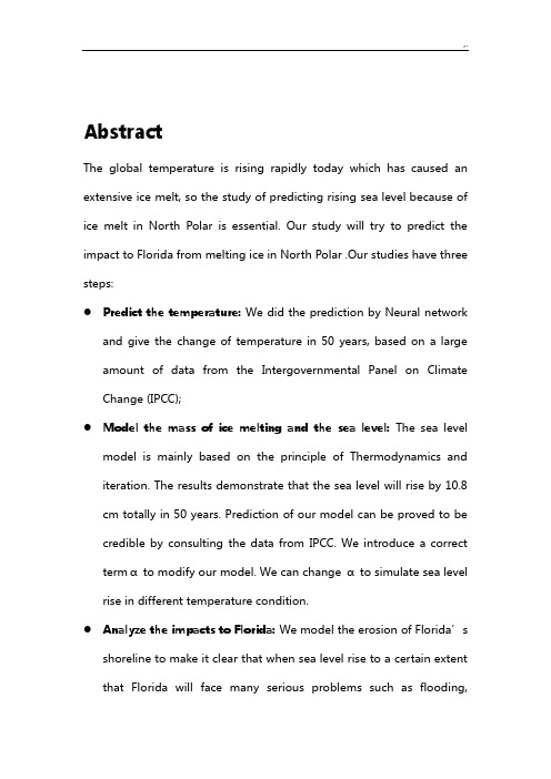
AbstractThe global temperature is rising rapidly today which has caused an extensive ice melt, so the study of predicting rising sea level because of ice melt in North Polar is essential. Our study will try to predict the impact to Florida from melting ice in North Polar .Our studies have three steps:●Predict the temperature: We did the prediction by Neural networkand give the change of temperature in 50 years, based on a large amount of data from the Intergovernmental Panel on Climate Change (IPCC);●Model the mass of ice melting and the sea level: The sea levelmodel is mainly based on the principle of Thermodynamics and iteration. The results demonstrate that the sea level will rise by 10.8 cm totally in 50 years. Prediction of our model can be proved to be credible by consulting the data from IPCC. We introduce a correct termαto modify our model. We can change αto simulate sea level rise in different temperature condition.●Analyze the impacts to Florida: We model the erosion of Florida’sshoreline to make it clear that when sea level rise to a certain extent that Florida will face many serious problems such as flooding,destruction of biodiversity, (Health Care), Loss of agriculture production (salinization of soil) and so on over the next 50 years.. We find the 17 cities or areas and 15 airports which are severely impacted by the rise of sea level.(Based on our results,) Without attaching more importance to solving the problem, shoreline of several coastal cities like Miami will be eroded seriously, and the lowest place−Key West will be disappeared.It will cost a huge financial loss, so further protection should be put into place.ContentIntroduction (4)Background (4)Our work (4)Study object: Ice cap in Greenland (4)Modeling the sea level (5)Analysis of Florida (5)Assumption (5)Model Ⅰ:Temperature Prediction (6)Grey Prediction Model: (6)Neural Network prediction Model: (6)Model Ⅱ:Melting ice and the rise of sea level (6)Model the rise of sea level (7)Heat from rise of temperature: (7)Mass of melting ice: (8)Design of Algorithms: (9)Model Results: Sea level will elevate by 10 centimeters in 50 years (10)Validation of our model: (11)Model ⅢAnalysis: The effects towards Florida (13)Major Cities Analysis (14)Miami (14)Tampa (15)Cape Coral (15)Key West (16)Other Impacts in Florida: (16)Recommendations to coastal Florida: (18)Judgments (18)Strengths (18)Weaknesses (19)Reference (20)IntroductionBackgroundGlobal Warming and sea level rise“Air temperatures at the top of the world continue to rise twice as fast as temperatures in lower latitudes, causing significant ice melt on land and sea”[Fears, December 17, 2014]. One of the serious consequences is that sea level will rise. Global average sea-level rose at an average rate of about 3.1[2.4 to 3.8] mm per year from 1993 to 2003[IPCC]. This information suggests that from 1993 to 2003 the sea-level rise by 3.1cm totally.Our workThe question requires us to predict the next 50 years’condition of ice melting and analyze the effects on the Florida, especially some big cities. So we can separate this question into two parts:●How much and how fast will the see level rise within 50 years?●What are the effects on the Florida because of the rise of sea level,especially some big cities?Study object: Ice cap in GreenlandArctic mainly consists of Greenland, which occupies about 9% glaciers all over the world. Melting in Arctic is mainly due to Greenland, melting of floating ice can be ignored. So we can consider Greenland as studyobject.Modeling the sea levelWe develop a model for sea-level rise as the function of time. This model can predict sea-level rise in future.Analysis of FloridaAfter having calculated the increased sea level within next 50 years, we analyze the impact to the Florida.●Rising sea level can seriously threaten the development of cities. Ithas been threatening some islands and coastal cities. Over the next18 years, about two thirds among 544 American towns will be twiceas likely to face floods [Huang]. More frequency hurricane will happen.●Sea water will corrode seacoast.● A large quantity of drinking water will be polluted. Assumption●Sea level rise is primarily due to the melting of ice cap in Green Land.We ignore the other floating ice in the Northern Polar.●The increment of sea water from melting will flow over the oceansuniformly●Salt in the ice will not affects the procedure of melting.Model Ⅰ:Temperature PredictionGrey Prediction Model:The weakness of the grey prediction is that the result is increasing all the time. In other words, it cannot show the changes in detail.Neural Network prediction Model:Model Ⅱ:Melting ice and the rise of sealevelModel the rise of sea levelThe main reason of the sea level rising is the melting of ice cap and the mass of melting ice is equal to the mass of sea water generated from melting. So, based on several physical principles, we model the rise of sea level by calculating the mass of melting ice. We assume that the increment of sea water from melting will flow over the world uniformly, which means the melting ice will contribute to the rise of sea level, divided by the area of the ocean.ρw V w=ρiV i=m i ∆x=V woV w The increment of sea water from melting iceV i The total volume of melting ice capV m The total volume of water generated from melting∆x The sea level riseS o The overall ocean area: 361745300km2, this is 71 percent of earth’s total surface area (Wikipedia).Heat from rise of temperature:According to the principle of thermal transmission, heat will always be transmitted from high temperature to low temperature. So, the final state of stuff in the thermal cycling system will reach to a same temperature. So, we assume that the temperature of the whole ice capwill increase by ∆T when the world temperature rise by ∆T. However, it takes time for the ice cap to transmit the heat from the rise temperature. We use the ∆T every month to calculate the increase of melting ice in each month and get the total increment by accumulation, which means parts of the heat from temperature will be absorbed and used to melt ice. So, defining a coefficient(α)and we will have the heat which ice cap absorbs from the rising temperature in the n-th month:Q n=αc i(m c−∆m i(n−1))∆T nQ n The heat comes from rises of temperature in the n-th monthαThe coefficient of capacity of absorbing heat in one monthc i The specific heat capacity of icem c The mass of the whole ice cap 2.45×10¹⁶kg∆m in The mass of melting ice in the n-th month∆T n The change of temperature in the n-th monthWe try to find the α by calculating the mass of melting ice in known years. “Recently reported GrIS mass balance varies from near-balance to modest mass losses [47 to 97 gigatons (Gt) year−1] in the 1990s, increasing to a mass loss of 267 ±38 Gt year−1 in 2007”(Michiel).α= 5.6735×10⁻³Mass of melting ice:The mass of melting ice in this month will depends on not only the rising temperature, but also the mass of melting ice in the last month.Wedivide the heat absorbed by the ice by the melting enthalpy of fusion for water to obtain the mass of extra melting ice resulted from the rise of temperature in this month.∆m in=∆m i(n−1)+Q n△fusHθmm i(k)=∑∆m in12kn=1∆m in The mass of melting ice in the n-th month△fusHθm: The melting enthalpy3.36×105J/kgm i(k)The total mass of melting ice in the next k yearsMoreover, “Since 2006, high summer melt rates have increased Greenland ice sheet mass loss to 273 gigatons per year”(Partitioning Recent Mass Loss). And the initial mass of melting ice in the first month will be calculated as follows:2.73×10¹⁴kg/12∆m i(−1)=m ii=2.73×101412kg∆x(k)=V wo=m i(k)ρwS om ii: The mass of melting ice in the initial year.∆x(k)The total rise of sea level in the next k yearsDesign of Algorithms:Since we have the function ∆m in=f(∆m i(n−1),∆T n), we are able to calculate the mass of melting ice in the next n months using computerprogram with the data of temperatures and the initial amount of melting ice in the first month.This is easy to achieve using two linear arrays ∆m i[]and ∆T[]in MATLAB. Run a simple for loop from 2 to n and calculate ∆m in during each pass so that the whole ∆m i[]array can be found.So that the total amount of melting ice at n-th month is the summation from ∆m i[1]to ∆m i[n]. Also the total rise of sea level can be easily found.Model Results: Sea level will elevate by 10 centimeters in 50 yearsThe solutions were coded using matlab:Figure 1: The mass of melting ice in the next 50 yearsFigure 2: The rise of sea level in the next 50 yearsThe prediction about rise of sea level every decade in next 50 years:∆x(10)=0.9874 cm∆x(20)=2.5125 cm∆x(30)=4.6222 cm∆x(40)=7.3674 cm∆x(50)= 10.8037 cmValidation of our model:The results show that the sea level will elevate by approximately 10 centimeters totally and 2 millimeters/yr, which accord with the prediction in Relative Mean Sea Level trends from NOAA.Moreover, if we calculated the rise of sea level without considering the increase of temperature, which means sea level rise at the rate today in the next 50 years, the order of magnitudes is match up with our result. So,based on the analysis above, the results of our modelModel ⅢAnalysis: The effects towards FloridaBased on our results, the sea level will rise 10 centimeters in the following 50 years, which threaten Florida in the future and result in tremendous impacts. “Some 2.4 million people and 1.3 million homes, nearly half the risk nationwide, sit within 4 feet of the local high tide line. Sea level rise is more than doubling the risk of a storm surge at this level in South Florida.”(Florida and rising sea)Figure 3 the altitudes of Florida ()As we can see from this picture, most cities or counties in the southern Florida lie besides the coast. Statistic suggests that 17 counties with altitudes smaller than 3 feet will be threatened by the rise of sea level in 50 years. The counties and airports which will be involved are listed as follows:Cities: Miami, Homestead, Fort Lauderdale, West Palm Beach, Titusville, St Augustine, Clearwater, St Petersburg, Tampa, Brandon, Bradenton, Port Charlotte,Cape Coral, Bonita Springs, Naples, Marco Island, and Grand Isle.Airports: Miami International Airport, Fort Lauderdale International Airport, Central Florida Regional Airport, Cedar Knoll Flying Ranch, Daytona Beach Regional Airport, Craig Municipal Airport, Jacksonville International Airport, St George Island Airport.Major Cities AnalysisWe choose 4 metropolises which will be severely impacted to do some further analysis.MiamiMiami is the biggest city in Florida with the average elevation of 3 feet(0.9144m) [15ikipedia]. Also, it is a coastal city. So according to what we predict that sea level will rise 10.8037cm within 50 years, we can draw a conclusion that this city would be greatly influenced.The possibility of flooding would grow while the frequency of hurricane will increase. It is a big challenge to sewer system of Miami. According to our simulation, sea level rising would also threaten Miami International Airport. Another problem is that the sea water would gnaw at the shoreline. Many coastal man-made buildings are too closed to the sea which they would face a serious problem of being eroded. Aside from threatening of losing habitat, local drinking water would be polluted.TampaTampa is a city located on the west coast of Florida. It is the third largest city in Florida. It is famous because of tourism. Although the highest point in the city is only 48 feet (15 m) [wikipedia], rising sea level will do harm to its natural disaster. Tampa is special because it has the Old Tampa Bay and Hillsborough Bay which is easy to be attacked by storm surge. Sea level rising would produce much more violent storm surge. The boundary of Tampa would also be lost. What’s more,Traffic facilities such as Tampa International Airport were under threatening of disappearing.Cape CoralThis city is famous because of its far-stretching beach and animated quay. Besides, it has more than 30 gardens and golf courses which attract many tourists. A variety of animals also promotes this city’s tourism. However, sea level rising would erode shoreline of Cape Coral. It would destroy natural environment of this area, and then damages biodiversity. And still worse, Pine Island would mostly disappear. So, the economic damage there will be hardly assessed.Key WestIt is an island of Florida, which have the lowest altitude. So if sea level rises to some extent, it would be the first to be under water.Other Impacts in Florida:Biodiversity: Wild life and rare animals in Florida will be impacted by loss of habitat and food. Moreover, it is hard for plants and animals in Florida to adapt the new climatic conditions and the increase of relative air humidity.Architecture:Sea level rise will cause salinization, which will impact the architectural production.Economy Pressure:More money will be put into the drainage systems and dam project, which means less city construction and business development.Health Care: Higher sea level will increase the risk of some disease like malaria.Recommendations to coastal Florida:●Build higher dams: In this way can cities hold back the rising floodwaters.●Prepare for flooding: Complete supervisory control system.Guarantee that citizen can be evacuated in time.●Reduce carbon emission: More carbon emission means highertemperature, and then lead to rising of sea level. So encouragecitizen to live a low-carbon life.●Warn local citizen: Propagate relative knowledge of sea level risingto improve citizen’s sense of self-protection when facing natural disaster.JudgmentsStrengths●We use Neural Network to predict temperature in future with a largeamount of reliable data. So our prediction of temperature in future is accurate relatively.●Our model can predict the sea level rising in different conditions,such as different temperature.●Our model is relatively simple so it will take a little time to simulate.We can easily get the result.Weaknesses●We ignore the areal variation about depth, salinity and temperature ofthe sea for simplifying the model;●We neglect the floating ice which will bring some error;●We neglect the thermal expansion;The mode is only the function of time, so it can’t simulate unusual situations.ReferenceBen Strauss,Florida and rising sea,/news/floria-and-the-rising-seaFears, Darryl, Huang, Ming. “Rising sea level threatens millions of American and causes huge economic loss”. Souhu, March 16, 2012, 09:48AM. Web.IPCC, http://www.ipcc.chMichiel van den Broeke,Partitioning Recent Mass Loss, Science 13 November 2009“National Snow and Ice Data Center”, January 7, 2015。
- 1、下载文档前请自行甄别文档内容的完整性,平台不提供额外的编辑、内容补充、找答案等附加服务。
- 2、"仅部分预览"的文档,不可在线预览部分如存在完整性等问题,可反馈申请退款(可完整预览的文档不适用该条件!)。
- 3、如文档侵犯您的权益,请联系客服反馈,我们会尽快为您处理(人工客服工作时间:9:00-18:30)。
2008MCM A 题 O 奖论文翻译
都会出现一些问题,包括: ·海岸线的侵蚀 ·水位线的升高 ·结构的不稳定 ·下水道的溢出 ·热带风暴的出现频率 ·排水系统的问题 以上问题中,基韦斯特和迈阿密是最容易受到影响的,而代顿海 滩和坦帕市相对来说是远离这些灾难的, 他们只是会或多或少的体验 到这么一些问题 海平面上升会带来一些潜在性的破坏结果;然而,采用有一些步 骤和措施可以有效避免和减轻破坏。 我们为佛罗里达抗击海平面上升 的影响提供了以下几中方法:提升公共意识、建设新建筑、抗击自然 灾害。 问题重述 我们在综合考虑了几个城市后, 分析了未来 50 年北极冰盖融化对 佛罗里达海岸的影响。这个问题可以被分解为以下两个到更多的问 题: ·融化率是多少,以及它对海平面上升的影响? ·海平面上升将会对佛罗里达的城市产生何种影响,以及人们如何消 除和抗击它? 我们的模型使用了表格 1 中的地球地理的数据,以及表格 2 中的
3 / 14
2008MCM A 题 O 奖论文翻译
和固体冰的密度分别为 1026 kg/m3 和 919 kg/m3。所以,如果这些浮 冰融化,原体积的 10%将会作为水注入海洋。因此,即使北极的冰盖 融化,对相对海平面上升也几乎没有影响。 冰盖 尽管冰盖的融化对海平面上升不会产生显著的影响,但如果他们 消失,以下几个问题确实会发生: ·北半球的海水平均温度将会有一个微小的下降 ·冰盖可以反射大量阳光,对降低区域温度有一定作用。一旦他们消 失,多余的能量将会被吸收,过一段时间以后,我们就可以看到全球 温度的一个显著升高,包括海洋和大气 陆地淡水冰 而陆地上的淡水冰融化并流入海洋,则是一种实实在在的增加。 格陵兰岛上冰的总体积大约是 2.624×10⁶ km3。如果这些冰全部融 化并流入海洋(不考虑洋底的升高和海洋表面积的增加) ,全球平均 海拔大概会上升 6.7 m,这是仅考虑格陵兰岛冰层的结果。 现在我们的问题就变成了: 在未来的 50 年里,陆地淡水冰的融化将会对海平面上升产生怎么样 的影响? 模型 1:常数模型 海平面上升的预测 为了预测冰盖融化对佛罗里达的影响,我们构建了一个可以快速 预测海平面上升状况的模型。其中,我们假设:
6 / 14
2008MCM A 题 O 奖论文翻译
Qx msT ,
其中, x 代表时间长度;
m 表示冰盖的质量; s 代表冰盖吸收热量的变化率;
T 全球温度的变Biblioteka 状况。计算发现Q50 4.85 1018 kJ
为了计算 50 内温度变化 0.7 摄氏度对淡水陆地冰融化状况的影 响,我们计算了被冰盖吸收的热量状况,0 摄氏度时 344kJ / kg ,将会 融化1.45 1016 kg 。 由于每立方米水的质量是 1000 千克, 海洋中增加的水总体积就是 把这些水平均分配在海洋平面上, 海平面将上升 4.0 cm 。 1.45 1016 m 3 。 模型一中,温海平面上升的高度达到 4.9 cm 。因此,在最好情况 下,50 年后海平面上升将达到 9 cm 。 最坏情况下:50 年内温度上升 2.9 度 使用同样的方法和方程, 可以计算得到最坏情况下 50 年后海平面 上升将达到 21 cm 。 模型 3:升温状况下的海洋体积变化 先前的两个模型在对待流入海洋的融化的淡水陆地冰的体积是不 考虑温度变化的。而且,这里也不考虑南半球和北半球相对面积。两 半球不同的海洋陆地面积比,也将对模型结果有一定影响。 北半球海洋面积
7 / 14
2008MCM A 题 O 奖论文翻译
北半球和南半球中海洋面积分别占全球海洋面积的 44%和 56% 。 【参考文献】 。也就说,北半球海洋面积大约是1.58 108 km2 。 冰盖融化后产生的水呆在北半球的比例 类似的冰盖融化状况在南半球也有发生。所以,南北球都有海平 面上升状况。关于海水流动状况的资料十分稀少。由于大部分冰盖融 化产生的水主要增加在海洋表层。这些水将会受到洋流的影响,所以 北极冰盖产生的水将会留在北半球。保守考虑,我们认为仅有大约一 半淡水陆地冰产生的水呆在北半球。 海洋温度上升造成的体积膨胀问题 对海洋温度上升的几个主要因素: ·上升的大气温度将提升海洋的温度 ·由于冰盖的融化,它们将反射更少的阳光,这意味着海洋将会吸收 更多的热量 ·更多的二氧化碳将会被海洋吸收 海平面以下 215 m 处,压力和阳光的因素将会使水温变化很少。 也就是说,只有海洋表层 215 m 的海水,将会受热产生体积膨胀。15 摄氏度时海水的体积变化率为 2.00 10 4 K 1 。我们通过以下的公式估 计最好和最坏的场景:
5 / 14
2008MCM A 题 O 奖论文翻译
的结果。为了得到一个更加现实和精确的结果,我们对模型进行了改 进。 模型 2:变温模型 我们的下一个模型考虑了温度变化对极区冰盖融化的影响。我们 将改变基本模型中假设极区温度不变的条件。 温度增长预测 20 世纪的全球平均温度大约上涨 1 摄氏度,但是过去 25 年温度 变化率已经接近于过去一个世纪的温度变化率。 【参考文献】另外, 额外排放的热量和二氧化碳气体将会被海洋吸收, 这将会直接提高海 洋温度。 因此,科学家已经预测未来 50 年全球温度将会上升 0.7 到 2.9 摄 氏度。 【参考文献】整体的温度上涨,将会加剧淡水陆地冰的融化速 度。相比于恒温模型,这将会增加海平面上升的程度。 我们将探讨未来 50 年温度上涨状况对海平面上升的影响。 模型分析 在分析了最好和最坏的场景之后,我们进行了线性化处理。例如, 最坏情况下,50 年内温度上涨 0.7 摄氏度,也就是每十年温度上涨 0.14 度。 最好情况下:50 年内温度上升 0.7 度 冰盖将会吸收更多的热量,融化更加快。以十年为计算单位,计 算海平面上升状况。 额外将被吸收得热量方程为
极区冰盖的初步讨论 极区冰盖主要分两种: ·像北极冰盖一样的固体海洋冰 ·主要分布在格陵兰、加拿大、阿拉斯加的淡水陆地冰 固体海洋冰 由于固体海洋冰一直漂浮在海面上,它的融化几乎对海平面的上 升无影响。根据阿基米德浮力定律,沉浸在液体中的物体受到液体对 它的与其重力相等的浮力。 海洋冰的大约 10%是露出水面的, 而海水
2008MCM A 题 O 奖论文翻译
北极冰盖融化的未来影响 The_impending_effects_of_ice_cap_melt
摘要 随着全球温度的不断提升,北极冰盖融化的问题也越来越广为关 注。 · 全球温度的升高在冰盖的融化以及世界海平面得上升中扮演着如 何的角色? ·伴随着海平面的上升,类似于佛罗里达区域中一些大都市在未来 50 年内又将面对何种问题? 我们建立了一个模型来回答上述问题: 构成北极冰盖大部分的浮冰融化不会影响海平面的变化,但发现 于格陵兰、 加拿大和阿拉斯加的淡水陆地冰的融化将对海平面上升产 生显著影响。我们的模型以目前淡水陆地冰的消耗率为切入点,并考 虑了以下几个问题 ·由于全球温度的升高造成冰盖融化率呈指数上升 ·北半球和南半球的相对陆海比 ·由于洋流原因,淡水陆地冰融化之后呆在北半球的比例 ·由于温度升高造成海洋表层体积热膨胀的问题 我们在分别分析了最好的和最坏的情况之后发现,在未来 50 年, 海平面相对的会上升 12 到 36 厘米。 为了说明这个上升结果造成的影响,我们分析了佛罗里达的四个 海岸城市:基韦斯特市、迈阿密市、代顿海滩市、坦帕市。很多方面
4 / 14
2008MCM A 题 O 奖论文翻译
·冰盖融化率为定值 ·冰盖融化所产生的水均匀分布在海洋表面 ·全球温度和气候没有显著的变化 我们使用了一下符号:
%Melt = 每十年陆地冰盖的融化比例 V 1 = 现阶段北半球陆地冰的体积
Ci w = 冰化成水体积转化状况 = 0.919
SAwo = 全球海洋表面积 = 3.611×10⁸ km3
在十年为一个时间单位下,方程转化为 海平面的上升度=
%Melt V 1 Ci w SAwo
从卫星图片所获得的数据显示, 格陵兰岛冰层每年约减少 239 km3 【参考文献】 。进行线性分析以后可知,50 年后海平面大约上升 3.3 cm。 我们必须考虑阿拉斯加和加拿大的冰层融化对海平面上升的影 响, 他们的融化将使海平面每年上升 0.025 cm 到 0.007 cm 之间。 【参 考文献】 。50 年后,他们造成海平面上升 1.6 cm 。所以,在 2058 年, 全球海平面上升约 4.9 cm,即 2 英尺。 对佛罗里达的到大都市的影响 由于所有的这些城市平均海拔都在 2 m 以上,所以,即使是 50 年后,海平面上升也不会对这些大都市产生显著的影响。然而,在面 对暴雨和飓风的时候,他们也将面临更多的洪水挑战。 然而,这些结果是在忽略一些影响海平面上升的充分条件时得出
9 / 14
2008MCM A 题 O 奖论文翻译
现一个海滨土地和一些迈阿密河沿岸小的损失轻微水浸。同样,由于 地下水位可能提出的问题,迈阿密应将有与饱满的下水道和排水系 统。然而,最大的问题之一期间可能出现的重大风暴,如飓风。随着 海洋增加高度和迈阿密市区低海拔,该城市的经验,长期持久洪水高 达36厘米水浸是目前最小的。 50年来,许多建筑物可以过于接近舒适的海洋,其结构的完整性可能 受到影响。 代托纳比奇市 代托纳比奇将会遇到一些海岸线的财产损失和在低洼地区更容易受 到洪水。此外,洪水的风险将会更加严重的热带风暴和飓风。然而, 由于是在海拔作为一个内陆急剧上升,洪水将可减至最低,城市排水 将保持相对正常。 坦帕市 坦帕市很少会遇到从目前形势的变化, 因为它的最低海拔在8米以上。 然而,坦帕必须准备更多的洪水和可能的排水问题。 佛罗里达海岸城市的共同问题 ·限制海岸侵蚀。在更多的侵蚀下,越滨海物业将会丢失。 · 监视水位。 由于海平面上升, 地下水位将影响建筑物和下水道基础。 可以限制内集的距离海岸建筑来监视水位。 ·准备水浸。高级海平面将产生更大的暴雨洪水。城市应制定撤离计 划和应急方案。 · 利用政府信息资源。 当谈到是否预测一个人体特别是城市中的危险,
Vchange Vstart B Tchange,