基于ANSYSWORKBENCH的保温桶的稳态热分析
ansysworkbench热分析研究教程

6-1A.几何模型B.组件-实体接触C.热载荷D.求解选项E.结果和后处理F. 作业6.1• 本节描述地应用一般都能在ANSYS DesignSpaceEntra或更高版本中使用,除了ANSYSStructural• 提示:在ANSYS 热分析地培训中包含了包括热瞬态分析地高级分析K T T= Q T –在稳态分析中不考虑瞬态影响–[K]可以是一个常量或是温度地函数–{Q}可以是一个常量或是温度地函数• 固体内部地热流(Fourier’s Law)是[K]地基础;• 热通量、热流率、以及对流在{Q}为边界条件;•对流被处理成边界条件,虽然对流换热系数可能与温度相关•在模拟时,记住这些假设对热分析是很重要地.–体、面、线•线实体地截面和轴向在DesignModeler中定义• 热分析里不可以使用点质量(PointMass)地特性•壳体和线体假设:–壳体:没有厚度方向上地温度梯度–线体:没有厚度变化,假设在截面上是一个常量温度• 但在线实体地轴向仍有温度变化唯一需要地材料特性是导热性(ThermalConductivity)•Thermal Conductivity在Engineering Data中输入•温度相关地导热性以表格形式输入若存在任何地温度相关地材料特性,就将导致非线性求解.–如果部件间初始就没有接触,那么就不会发生热传导(见下面对pinball地解释).–总结:–Pinball区域决定了什么时候发生接触,并且是自动定义地,同时还给了一个相对较小地值来适应模型里地小间距.• 默认情况下,假设部件间是完美地热接触传导,意味着界面上不会发生温度实际情况下,有些条件削弱了完美地热接触传导:TTx⋅ (T q = TCC target - T conta ct – 式中T contact 是一个接触节点上地温度, T target 是对应目标节点上地温度–默认情况下,基于模型中定义地最大材料导热性KXX 和整个几何边界框地对角线ASMDIAG ,TCC 被赋以一个相对较大地值.TCC = KXX ⋅10,000/ ASMDIAG– 这实质上为部件间提供了一个完美接触传导• 在ANSYS Professional或更高版本,用户可以为纯罚函数和增广拉格朗日方程定义一个有限热接触传导(TCC).–在细节窗口,为每个接触域指定TCC输入值–如果已知接触热阻,那么它地相反数除以接触面积就可得到TCC值–Spotweld在CAD软件中进行定义(目前只有DesignModeler和Unigraphics 可用).T2 T1热流量: – 热流速可以施加在点、边或面上.它分布在多个选择域上.– 它地单位是能量比上时间(energy/time )•完全绝热(热流量为0): •热生成:– 内部热生成只能施加在实体上– 它地单位是能量比上时间在除以体积(energy/time/volume )正地热载荷会增加系统地能量.– 可以删除原来面上施加地边界条件• 热通量:– 热通量只能施加在面上(二维情况时只能施加在边上)– 它地单位是能量比上时间在除以面积( e nergy/time/area )温度、对流、辐射:•完全绝热条件将忽略其它地热边界条件 • 给定温度: – 给点、边、面或体上指定一个温度– 温度是需要求解地自由度• 至少应存在一种类型地热边界条件,否则,如果热量将源源不断地输入到系统中,稳态时地温度将会达到无穷大.• 另外,给定地温度或对流载荷不能施加到已施加了某种热载荷或热边界条件地表面上 .•对流:– 只能施加在面上(二维分析时只能施加在边上)– 对流q 由导热膜系数 h ,面积A ,以及表面温度T surface 与环境温度T ambient 地差值 来定义. q = hA (T surface - T ambient )– “h ” 和 “T ambient ” 是用户指定地值– 导热膜系数 h 可以是常量或是温度地函•与温度相关地对流:–为系数类型选择Tabular(Temperature)–输入对流换热系数-温度表格数据–在细节窗口中,为h(T)指定温度地处理方式•几种常见地对流系数可以从一个样本文件中导入.新地对流系数可以保存在文件中.•辐射:– 施加在面上(二维分析施加在边上)(4 4)– 式中: Q R = σεFAT surface - T ambient• σ=斯蒂芬一玻尔兹曼常数• ε =放射率• A =辐射面面积• F = 形状系数(默认是1)– 只针对环境辐射,不存在于面面之间(形状系数假设为1)– 斯蒂芬一玻尔兹曼常数自动以工作单位制系统确定在projectschematic里建立一个SSThermalsystem(SS热分析)•在Mechanical 里,可以使用Analysis Settings为热分析设置求解选项.–注意,第四章地静态分析中地AnalysisDataManagement选项在这里也可以使用.加地结构载荷和约束.– 求解结构在Static Structural 中插入了一个importedload 分支,并同时导入了施–温度–热通量–反作用地热流速–用户自定义结果•模拟时,结果通常是在求解前指定,但也可以在求解结束后指定.–搜索模型求解结果不需要在进行一次模型地求解.– 温度是标量,没有方向– 热通量 q 定义为q = -KXX ⋅∇TTotal Heat Flux (整体热通量)和DirectionalHeatFlux (方向热通量)–通过插入probe指定响应热流量,或–用户可以交替地把一个边界条件拖放到Solution上后搜索响应•作业6.1–稳态热分析•目标:–分析图示泵壳地热传导特性版权申明本文部分内容,包括文字、图片、以及设计等在网上搜集整理.版权为个人所有This article includes some parts, including text, pictures, and design. Copyright is personal ownership.用户可将本文地内容或服务用于个人学习、研究或欣赏,以及其他非商业性或非盈利性用途,但同时应遵守著作权法及其他相关法律地规定,不得侵犯本网站及相关权利人地合法权利.除此以外,将本文任何内容或服务用于其他用途时,须征得本人及相关权利人地书面许可,并支付报酬.Users may use the contents or services of this article for personal study, research or appreciation, and othernon-commercial or non-profit purposes, but at the same time, they shall abide by the provisions of copyright law and other relevant laws, and shall not infringe upon the legitimate rights of this website and its relevant obligees. In addition, when any content or service of this article is used for other purposes, written permission and remuneration shall be obtained from the person concerned and the relevant obligee.转载或引用本文内容必须是以新闻性或资料性公共免费信息为使用目地地合理、善意引用,不得对本文内容原意进行曲解、修改,并自负版权等法律责任.Reproduction or quotation of the content of this article must be reasonable and good-faith citation for the use of news or informative public free information. It shall not misinterpret or modify the original intention of the content of this article, and shall bear legal liability such as copyright.。
ANSYS热分析指南——ANSYS稳态热分析word精品文档59页

ANSYS热分析指南(第三章)第三章稳态热分析3.1稳态传热的定义ANSYS/Multiphysics,ANSYS/Mechanical,ANSYS/FLOTRAN和ANSYS/Professional这些产品支持稳态热分析。
稳态传热用于分析稳定的热载荷对系统或部件的影响。
通常在进行瞬态热分析以前,进行稳态热分析用于确定初始温度分布。
也可以在所有瞬态效应消失后,将稳态热分析作为瞬态热分析的最后一步进行分析。
稳态热分析可以计算确定由于不随时间变化的热载荷引起的温度、热梯度、热流率、热流密度等参数。
这些热载荷包括:对流辐射热流率热流密度(单位面积热流)热生成率(单位体积热流)固定温度的边界条件稳态热分析可用于材料属性固定不变的线性问题和材料性质随温度变化的非线性问题。
事实上,大多数材料的热性能都随温度变化,因此在通常情况下,热分析都是非线性的。
当然,如果在分析中考虑辐射,则分析也是非线性的。
3.2热分析的单元ANSYS和ANSYS/Professional中大约有40种单元有助于进行稳态分析。
有关单元的详细描述请参考《ANSYS Element Reference》,该手册以单元编号来讲述单元,第一个单元是LINK1。
单元名采用大写,所有的单元都可用于稳态和瞬态热分析。
其中SOLID70单元还具有补偿在恒定速度场下由于传质导致的热流的功能。
这些热分析单元如下:表3-1二维实体单元表3-2三维实体单元表3-3辐射连接单元表3-4传导杆单元表3-5对流连接单元表3-6壳单元表3-7耦合场单元表3-8特殊单元3.3热分析的基本过程ANSYS热分析包含如下三个主要步骤:前处理:建模求解:施加荷载并求解后处理:查看结果以下的内容将讲述如何执行上面的步骤。
首先,对每一步的任务进行总体的介绍,然后通过一个管接处的稳态热分析的实例来引导读者如何按照GUI路径逐步完成一个稳态热分析。
最后,本章提供了该实例等效的命令流文件。
ANSYS稳态热分析的基本过程和实例
ANSYS稳态热分析的基本过程ANSYS热分析可分为三个步骤:•前处理:建模、材料和网格•分析求解:施加载荷计算•后处理:査看结果1、建模①、确定jobname> title、unit;②、进入PREP7前处理,定义单元类型,设定单元选项;③、定义单元实常数;④、定义材料热性能参数,对于稳态传热,一般只需定义导热系数,它可以是恒定的,也可以随温度变化;⑤、创建儿何模型并划分网格,请参阅《ANSYS Modeling and Meshing Guide》。
2、施加载荷计算①、定义分析类型•如果进行新的热分析:Command: ANTYPE, STATIC, NEWGUI: Main menu>Solution>-Analysis Type->New Analysis>Steady-state•如果继续上一次分析,比如增加边界条件等:Command: ANTYPE, STATIC, RESTGUI: Main menu>Solution>Analysis Type->Restart②、施加载荷可以直接在实体模型或单元模型上施加五种载荷(边界条件):a、恒定的温度通常作为自由度约束施加于温度已知的边界上。
Command Family: DGUI: Main Menu>Solution>-Loads-Apply>-Thermal-Temperatureb、热流率热流率作为节点集中载荷,主要用于线单元模型中(通常线单元模型不能施加对流或热流密度载荷),如果输入的值为正,代表热流流入节点,即单元获取热量。
如果温度与热流率同时施加在一节点上则ANSYS读取温度值进行计算。
注意:如果在实体单元的某一节点上施加热流率,则此节点周用的单元要密一些,在两种导热系数差别很大的两个单元的公共节点上施加热流率时, 尤其要注意:。
此外,尽可能使用热生成或热流密度边界条件,这样结果会更精确些。
ANSYS Workbench 17·0有限元分析:第12章-热分析
第12章 热分析 热力学分析(简称热分析)用于计算一个系统或部件的温度分布及其他各种热物理参数,如热量的获取与损失、热梯度、热流密度(热通量)等。
热分析在许多工程应用中扮演着非常重要的角色,如内燃机、涡轮机、换热器、电子元件等。
★ 了解传热的基础知识。
12.1 传热概述传热分析(Steady-State Thermal Analysis )遵循热力学第一定律,即能量守恒定律。
对于一个封闭的系统(没有质量的流入或流出),则:PE KE U W Q Δ+Δ+Δ=−式中Q 为热量,W 为所做的功,ΔU 为系统的内能,KE Δ为系统的动能,PE Δ为系统的势能。
对于大多数工程传热问题:0==PE KE ΔΔ若不考虑做功,即0=W ,则U Q Δ=;对于稳态热分析:0=Δ=U Q即流入系统的热量等于流出的热量;对于瞬态热分析:q dU dt =即流入或流出的热传递速率q 等于系统内能的变化。
12.1.1 传热方式热分析包括热传导、热对流、热辐射三种传热方式。
ANSYS Workbench 17.0有限元分析从入门到精通1.热传导热传导可以定义为完全接触的两个物体之间,或一个物体的不同部分之间由于温度梯度而引起的内能交换。
热传导遵循傅里叶定律:dxdT k q −=′′ 式中q ′′为热流密度(W/m 2),k 为导热系数。
2.热对流热对流是指固体的表面与它周围接触的流体之间,由于温差的存在引起的热量交换。
热对流可以分为两类:自然对流和强制对流。
热对流用牛顿冷却方程来描述:)(B T S T h q −=′′ 式中h 为对流换热系数(或称膜传热系数、给热系数、膜系数等),S T 为固体表面的温度,B T 为周围流体的温度。
3.热辐射热辐射是指物体发射电磁能,并被其他物体吸收转变为热的热量交换过程。
物体温度越高,单位时间内辐射的热量就越多。
热传导和热对流都需要有传热介质,而热辐射无须任何介质。
实质上,在真空中的热辐射效率最高。
基于AnsysWorkbench的保温运输箱体设计
基于Ansys Workbench的保温运输箱体设计发布时间:2021-09-15T07:17:23.121Z 来源:《科技新时代》2021年6期作者:邓连辉黄斌罗端华胡志坚[导读] 使其严格控制在一定变形范围内,以保证整个系统的良好工作[1-3]。
(衡阳泰豪通信车辆有限公司湖南衡阳421001 )摘要:本文描述了一种可以在多载具条件下实现的保温运输箱体,采用碳纤维复合材料定制保温运输箱体既可以满足载具承载要求,又可以有效减重。
为保证保温运输箱体在多种工况条件下的强度和刚度,对其进行有限元计算。
基于复合材料层合板理论,建立保温运输箱体的碳纤维复合材料等效杨氏模量模型,再基于等效杨氏模量代入Ansys Workbench中进行有限元计算。
结果表明,保温运输箱体在多种工况条件下可保证其稳定性和可靠性。
关键词:保温运输箱体、碳纤维复合材料、等效杨氏模量、Ansys Workbench1.概述保温运输箱体用于装载恒温物件,且能在多种运输载具下实现。
由于运输载具不同,所以保温运输箱体的承载工况也不尽相同,且保温运输箱体内装载物件有严格的尺寸精度要求,所以必须考虑在各种承载工况下保温运输箱体的变形情况,使其严格控制在一定变形范围内,以保证整个系统的良好工作[1-3]。
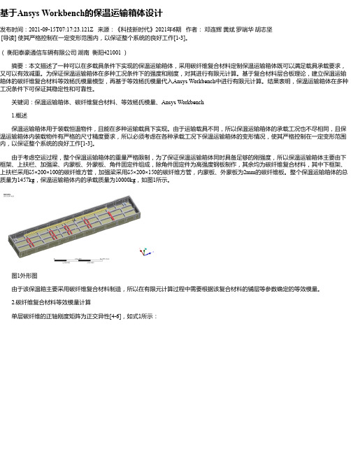
由于考虑空运过程,整个保温运输箱体的重量严格限制,为了保证保温运输箱体同时具备足够的刚强度,所以保温运输箱体主要由下框架、上扶栏、加强梁、内蒙板、外蒙板、角件固定件组成,除角件固定件为高强度钢板制作,其余均为碳纤维复合材料,其中下框架、上扶栏采用δ5×200×100的碳纤维方管,加强梁采用δ5×200×150的碳纤维方管,内蒙板、外蒙板为2mm的碳纤维板。
整个保温运输箱体的总质量为1457kg,保温运输箱体内的承载质量为10000kg,如图1所示。
图1外形图由于该保温箱主要采用碳纤维复合材料制造,所以在有限元计算过程中需要根据该复合材料的铺层等参数确定的等效模量。
ansys稳态热力学分析的基本过程及注意要点
ansys稳态热力学分析的基本过程及注意要点1. ansys热力学分析的基本过程及注意要点1.1,对于稳态分析,一般只需要定义导热系数,它可以是恒定的,也可以是随温度变化的。
1.2,在分析过程中,不一定选择国际单位制,但是在建立几何模型及输入材料热性参数时,单位必须统一。
2. ansys中提供6种热载荷:温度(temperature),热流率(heat flow),对流(convection),热流密度(heat flux),生热率(heat generate),辐射率(radiation)。
2.1 温度载荷2.1.1 在单个或者多个节点上施加温度载荷main menu/solution/define loads/apply/thermal/temperature/on nodes2.1.2 在所有节点上施加均匀温度载荷main menu/solution/define loads/apply/thermal/temperature/uniform tempmain menu/solution/define loads/setting /uniform tempmain menu/solution/loading options/uniform temp2.1.3 在关键点上施加温度载荷main menu/solution/define loads/apply/thermal/ temperature/on keypoints 2.1.4 在线段上施加温度载荷main menu/solution/define loads/apply/thermal/temperature/on lines2.1.5 在面上施加温度载荷main menu /solution/define loads/apply /thermal/ temperature/ on areas 2.2 热流率载荷2.2.1 在节点上施加热流率载荷main menu/solution/define loads/apply/thermal/heat flow/on nodes2.2.2 在关键点上施加热流率载荷2.3 对流载荷(convection)2.3.1在节点上施加对流载荷main menu/solution/define loads /apply/thermal/ convection/ on nodes2.3.2 在单元上施加均匀对流载荷mani menu/solution/ define loads/ apply /thermal/ convection /on elements/ uniform2.3.3 在单元上施加非均匀对流载荷mani menu/solution/ define loads/ apply /thermal/ convection /on elements/ tapered2.3.4 在线段上施加对流载荷main menu/solution/ define loads/ apply/ thermal/ convection/on lines2.3.5 在面上施加对流载荷main menu/ solution/ define loads/ apply /thermal/ convection/on areas2.4 热流密度载荷(heat flux)2.4.1 在节点上施加热流密度载荷main menu/ solution/ define loads/apply/ thermal/ heat flux/ on nodes2.4.2 在单元上施加热流密度载荷main menu/ solution/deine loads/apply thermal/heat flux / on elements2.4.3 在线段上施加热流密度载荷main menu/ solution /define loads/ apply / thermal/ heat flux/ on lines2.4.4 在面上施加热流密度载荷main menu/solution/ define loads /apply/ thermal/ heat flux/ on areas2.5 生热率载荷(heat generate)2.5.1 在节点上施加生热密度载荷main menu/solution/define loads /apply/ thermal/ heat generate/ on nodes 2.5.2 在所有节点施加均匀生热流密度载荷main menu / solution/ define loads /apply /thermal/ heat generate/ uniform heat generate2.5.3 在线段上施加生热密度载荷main menu / solution/ define loads /apply /thermal/ heat generate/on lines 2.5.4 在面上施加生热密度载荷main menu / solution/ define loads /apply /thermal/ heat generate/on areas 2.5.5 在体上施加生热密度载荷main menu / solution/ define loads /apply /thermal/ heat generate/on volumes 2.6 辐射率载荷(radiation)2.6.1 在节点上施加辐射率载荷main menu/ solution /define loads/ apply /thermal /radiation/ on Nodes2.6.2 在单元上施加辐射率载荷main menu/ solution /define loads/ apply /thermal /radiation/ on elements 2.6.3 在线段上施加辐射率载荷main menu/ solution /define loads/ apply /thermal /radiation/ on lines2.6.4 在面上施加辐射率载荷main menu/ solution /define loads/ apply /thermal /radiation/on areas3 稳态求解选项设置在对一个稳态热分析问题时,需要设置time/frequence选项、非线性选项以及输出控制等载荷步选项3.1 time-time step该选项用于设置载荷步的时间main menu/solution/loads step opts/ time&frequence/time -time step3.2 time and substeps该选项用于确定每载荷步中子步的数量或者时间步大小main menu/ solution/ load step options/ time & frequence/ time and substeps 3.3 convergence criteria该选项可根据温度、热流率等指标设置热分析的收敛标准,检验热分析的收敛性。
最新ANSYS热分析指南——ANSYS稳态热分析
A N S Y S热分析指南——A N S Y S稳态热分析ANSYS热分析指南(第三章)第三章稳态热分析3.1稳态传热的定义ANSYS/Multiphysics,ANSYS/Mechanical,ANSYS/FLOTRAN和ANSYS/Professional这些产品支持稳态热分析。
稳态传热用于分析稳定的热载荷对系统或部件的影响。
通常在进行瞬态热分析以前,进行稳态热分析用于确定初始温度分布。
也可以在所有瞬态效应消失后,将稳态热分析作为瞬态热分析的最后一步进行分析。
稳态热分析可以计算确定由于不随时间变化的热载荷引起的温度、热梯度、热流率、热流密度等参数。
这些热载荷包括:对流辐射热流率热流密度(单位面积热流)热生成率(单位体积热流)固定温度的边界条件稳态热分析可用于材料属性固定不变的线性问题和材料性质随温度变化的非线性问题。
事实上,大多数材料的热性能都随温度变化,因此在通常情况下,热分析都是非线性的。
当然,如果在分析中考虑辐射,则分析也是非线性的。
3.2热分析的单元ANSYS和ANSYS/Professional中大约有40种单元有助于进行稳态分析。
有关单元的详细描述请参考《ANSYS Element Reference》,该手册以单元编号来讲述单元,第一个单元是LINK1。
单元名采用大写,所有的单元都可用于稳态和瞬态热分析。
其中SOLID70单元还具有补偿在恒定速度场下由于传质导致的热流的功能。
这些热分析单元如下:表3-1二维实体单元表3-2三维实体单元表3-3辐射连接单元表3-4传导杆单元表3-5对流连接单元表3-6壳单元表3-7耦合场单元表3-8特殊单元3.3热分析的基本过程ANSYS热分析包含如下三个主要步骤:前处理:建模求解:施加荷载并求解后处理:查看结果以下的内容将讲述如何执行上面的步骤。
首先,对每一步的任务进行总体的介绍,然后通过一个管接处的稳态热分析的实例来引导读者如何按照GUI路径逐步完成一个稳态热分析。
ansys workbench热分析报告教程

6-1•本章练习稳态热分析的模拟,包括:A.几何模型B.组件-实体接触C.热载荷D.求解选项E.结果和后处理F. 作业6.1•本节描述的应用一般都能在ANSYS DesignSpaceEntra或更高版本中使用,除了ANSYSStructural•提示:在ANSYS 热分析的培训中包含了包括热瞬态分析的高级分析•对于一个稳态热分析的模拟,温度矩阵{T}通过下面的矩阵方程解得:•假设:KT TQ T–在稳态分析中不考虑瞬态影响–[K]可以是一个常量或是温度的函数–{Q}可以是一个常量或是温度的函数•上述方程基于傅里叶定律:•固体内部的热流(Fourier’s Law)是[K]的基础;•热通量、热流率、以及对流在{Q}为边界条件;•对流被处理成边界条件,虽然对流换热系数可能与温度相关•在模拟时,记住这些假设对热分析是很重要的。
•热分析里所有实体类都被约束:–体、面、线•线实体的截面和轴向在DesignModeler中定义•热分析里不可以使用点质量(PointMass)的特性•壳体和线体假设:•唯一需要的材料特性是导热性(ThermalConductivity)•Thermal Conductivity在Engineering Data中输入•温度相关的导热性以表格形式输入•对于结构分析,接触域是自动生成的,用于激活各部件间的热传导–如果部件间初始就已经接触,那么就会出现热传导。
–如果部件间初始就没有接触,那么就不会发生热传导(见下面对pinball的解释)。
–总结:–Pinball区域决定了什么时候发生接触,并且是自动定义的,同时还给了一个相对较小的值来适应模型里的小间距。
•如果接触是Bonded(绑定的)或noseparation (无分离的),那么当面出现在pinballradius内时就会发生热传导(绿色实线表示)。
PinballRadius右图中,两部件间的间距大于pinball 区域,因此在这两个部件间会发生热传导。
基于ANSYSWORKBENCH的保温桶的稳态热分析
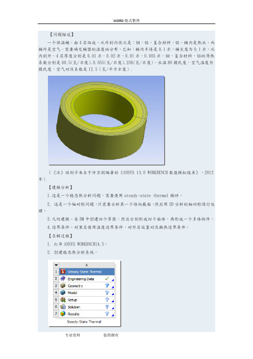
【问题描述】一个保温桶,由4层组成。
从外到内依次是:钢,铝,复合材料,铝。
桶内是热水,而桶外是空气。
需要确定桶壁的温度场分布。
已知:桶内半径是0.1米,桶长度为0.1米,从内到外,4层厚度分别是0.01米,0.02米,0.01米,0.005米,钢,复合材料,铝的导热系数分别是60.5(瓦/米度),0.055(瓦/米度),236(瓦/米度),水温80摄氏度,空气温度为摄氏度,空气对流系数是12.5(瓦/平方米度).(《注》该例子来自于许京荆编著的《ANSYS 13.0 WORKBENCH数值模拟技术》,2012年)【建模分析】1.这是一个稳态热分析问题,需要使用steady-state thermal模块。
2. 这是一个轴对称问题,只需要分析其一个径向截面,然后用2D分析的轴对称进行处理。
3.几何建模。
在DM中创建四个草图,然后分别形成四个面体,再形成一个多体构件。
4.边界条件。
对里层使用温度边界条件,对外层设置对流换热边界条件。
【求解过程】1. 打开ANSYS WORKBNCH14.5。
2. 创建稳态热分析系统。
3. 设置三种材料的导热系数。
双击engineering data,打开工程数据,新创建三种材料,分别是STEEL,AL,compound,并分别设置其导热系数。
钢材的导热系数铝的导热系数复合材料的导热系数创建完毕,退回到项目中。
4.创建几何模型。
双击geometry,进入到DM中。
选择长度的单位是米。
在XOY面内创建四个草图。
这四个草图是四个相邻的矩形,其位置及尺寸如下图。
分别由这4个草图生成4个面。
其图形如下将上述四个物体生成一个多体构件。
几何建模结束,存盘,退出DM.然后设置几何体的属性是2D,表明下面准备做的是2D分析。
5.为各几何体分配材料。
双击model,进入到mechanical.首先选中geometry,在其属性栏中设置是做轴对称分析。
然后为各个几何4体分配材料。
6.划分网格。
ANSYS workbench稳态及瞬态热分析

b. 网格控制:在Details of “Mesh ” 中单击sizing,size function选择 Proximity and Curvature(临近 以及曲率)选项
c. 选中Mesh,单击鼠标右键
→Generate Mesh
c
1
稳态热分析实例
划分网格 e. 对于曲面模型使用Proximity and Curvature(临近以及曲率)网格控制会
k导热系数(W/(m·℃)),q二次导数为热流密度(W/m^2)
1
热分析简介
基本的传热方式:热传导、热对流、热辐射、相变 2. 热对流(Convection) 对流是指温度不同的各个部分流体之间发生相对运动所引起的热量传递方 式。 热对流满足牛顿冷却方程:
q" h(Ts Tb)
q"为热流密度; h为物质的对流传热系数 ; TS是固体的表面温度; Tb为周围流体温度。
(续)
1
流程简介ቤተ መጻሕፍቲ ባይዱ
材料属性
1
流程简介
装配体与接触
•对于复杂的装配体模型,如果零件初始不接触将不会互相传热
•如果初始有接触就会发生传热
•对于不同的接触类型,将会决定接触面以及目标面之间是否会发生热量传递。 可以利用pinball调整模型可能出现的 间隙,如下表所示:
接触类型
•节点位于Pinball 内:
Mechanical。选中模型树 Geometry 下模型1 2. 在Detail of “1”中,展开Material选 项,单击Assignment后三角 3. 在下拉菜单中选择Copper Alloy
1
稳态热分析实例
划分网格 a. 首先使用程序自动划分网格,查
ansys workbench稳态热分析

Workbench -Mechanical Introduction Introduction作业6.1稳态热分析作业6.1 –目标Workshop Supplement •本作业中,将分析下图所示泵壳的热传导特性。
•确切说是分析相同边界条件下的塑料(Polyethylene)泵壳和铝(Aluminum)泵壳。
)泵壳•目标是对比两种泵壳的热分析结果。
作业6.1 –假设Workshop Supplement 假设:•泵上的泵壳承受的温度为60度。
假设泵的装配面也处于60度下。
•泵的内表面承受90度的流体。
•泵的外表面环境用一个对流关系简化了的停滞空气模拟,温度为20度。
作业6.1 –Project SchematicWorkshop Supplement •打开Project 页•从Units菜单上确定:–项目单位设为Metric (kg, mm, s, C, mA, mV)–选择Display Values in Project Units…作业6.1 –Project SchematicWorkshop Supplement 1.在Toolbox中双击Steady-State Thermal创建一个新的Steady State Thermal(稳态Steady State Thermal热分析)系统。
1.2.在Geometry上点击鼠标右键选择p y,导入文Import Geometry件Pump_housing.x_t 2.…作业6.1 –Project SchematicWorkshop Supplement3.双击Engineering Data得到materialproperties(材料特性) 3.4.选中General Materials的同时,点击Aluminum Alloy和Polyethylene旁边的‘+’符号,把它们添加到项目中。
5.Return to Project(返回到项目)4.5.Workshop Supplement…作业6.1 –Project Schematic6.把Steady StateThermal 拖放到第一个系统的Geometry 上。
ansys workbench热分析教程

•本章练习稳态热分析的模拟,包括:A. 几何模型B. 组件-实体接触C. 热载荷D. 求解选项E. 结果和后处理F. 作业6.1• 本节描述的应用一般都能在ANSYS DesignSpace Entra或更高版本中使用,除了ANSYS Structural• 提示:在ANSYS 热分析的培训中包含了包括热瞬态分析的高级分析•对于一个稳态热分析的模拟,温度矩阵{T}通过下面的矩阵方程解得:[K(T)]{T}= {Q(T )}•假设:–在稳态分析中不考虑瞬态影响–[K] 可以是一个常量或是温度的函数–{Q}可以是一个常量或是温度的函数•上述方程基于傅里叶定律:• 固体内部的热流(Fourier’s Law)是[K]的基础;• 热通量、热流率、以及对流在{Q} 为边界条件;•对流被处理成边界条件,虽然对流换热系数可能与温度相关•在模拟时,记住这些假设对热分析是很重要的。
•热分析里所有实体类都被约束:–体、面、线•线实体的截面和轴向在D esignModeler中定义• 热分析里不可以使用点质量(Point Mass)的特性•壳体和线体假设:–壳体:没有厚度方向上的温度梯度–线体:没有厚度变化,假设在截面上是一个常量温度• 但在线实体的轴向仍有温度变化• 唯一需要的材料特性是导热性(Thermal Conductivity )• Thermal Conductivity 在 Engineering Data 中输 入• 温度相关的导热性以表格 形式输入若存在任何的温度相关的材料特性,就将导致非线性求解。
… 材料特性Training ManualB. 组件-实体接触Training Manual•对于结构分析,接触域是自动生成的,用于激活各部件间的热传导–如果部件间初始就已经接触,那么就会出现热传导。
–如果部件间初始就没有接触,那么就不会发生热传导(见下面对pinball的解释)。
–总结:–Pinball区域决定了什么时候发生接触,并且是自动定义的,同时还给了一个相对较小的值来适应模型里的小间距。
ANSYS Workbench 热分析教程

图 3-1 平行平板辐射模型
3.2. 问题分析
该问题为稳态辐射换热问题,分析思路如下: 1. 2. 3. 4. 5. 6. 7. 8. 选择稳态热分析系统。 确定材料参数:稳态辐射换热问题,仅输入平板导热系数。 【DesignModeler】建立两平板几何模型。 进入【Mechanical】分析程序。 网格划分:采用系统默认网格。 施加边界条件:平板四周对称面无热量交换,为绝热边界,系统默认无需输入,环 境温度 20℃。 设置需要的结果:温度分布。 求解及结果显示。
图 2-2 建立保温桶分析文件
2、确定材料参数(图 2-3) 1) 编辑工程数据模型,添加材料的导热率,右击鼠标选择【Engineering Data】 【Edit】 2) 工程数据属性中增加新材料: 【Outline of Schematic A2:Engineering Data】 【Click here to add new material】输入材料名称 Aluminium 3) 选择【Thermal】 【Isotropic Thermal Conductivity】 4) 选择铝材料属性【Properties of Outline Row 3: Aluminium】 【Isotropic Thermal Conductivity】 5) 出现【Table of Properties Row 2: Thermal Conductivity】材料属性表,双击鼠标, 点击每个区域输入材料属性参数:温度 20℃,导热率 236W/(m·℃)。 6) 参数输完后,工程数据表显示导热率-温度图表。 7) 同样输入树脂基复合材料热传导率 0.055W/(m· ℃)。 8) 同样输入钢材料热传导率 70W/(m·℃)。
图 2-12 施加内层表面温度
【VIP专享】ANSYS稳态和瞬态分析步骤简述

ANSYS 稳态和瞬态热模拟基本步骤基于ANSYS 9.0一、稳态分析从温度场是否是时间的函数即是否随时间变化上,热分析包括稳态和瞬态热分析。
其中,稳态指的是系统的温度场不随时间变化,系统的净热流率为0,即流入系统的热量加上系统自身产生的热量等于流出系统的热量:=0q q q+-流入生成流出在稳态分析中,任一节点的温度不随时间变化。
基本步骤:(为简单起见,按照软件的菜单逐级介绍)1、选择分析类型点击Preferences 菜单,出现对话框1。
对话框1我们主要针对的是热分析的模拟,所以选择Thermal 。
这样做的目的是为了使后面的菜单中只有热分析相关的选项。
2、定义单元类型GUI :Preprocessor>Element Type>Add/Edit/Delete 出现对话框2对话框2(3-1)点击Add,出现对话框3对话框3在ANSYS中能够用来热分析的单元大约有40种,根据所建立的模型选择合适的热分析单元。
对于三维模型,多选择SLOID87:六节点四面体单元。
3、选择温度单位默认一般都是国际单位制,温度为开尔文(K)。
如要改为℃,如下操作GUI:Preprocessor>Material Props>Temperature Units选择需要的温度单位。
4、定义材料属性对于稳态分析,一般只需要定义导热系数,他可以是恒定的,也可以随温度变化。
GUI: Preprocessor>Material Props> Material Models 出现对话框4对话框4一般热分析,材料的热导率都是各向同性的,热导率设定如对话框5.对话框5若要设定材料的热导率随温度变化,主要针对半导体材料。
则需要点击对话框5中的Add Temperature选项,设置不同温度点对应的热导率,当然温度点越多,模拟结果越准确。
设置完毕后,可以点击Graph按钮,软件会生成热导率随温度变化的曲线。
稳态热分析案例(ANSYS 15.0版)
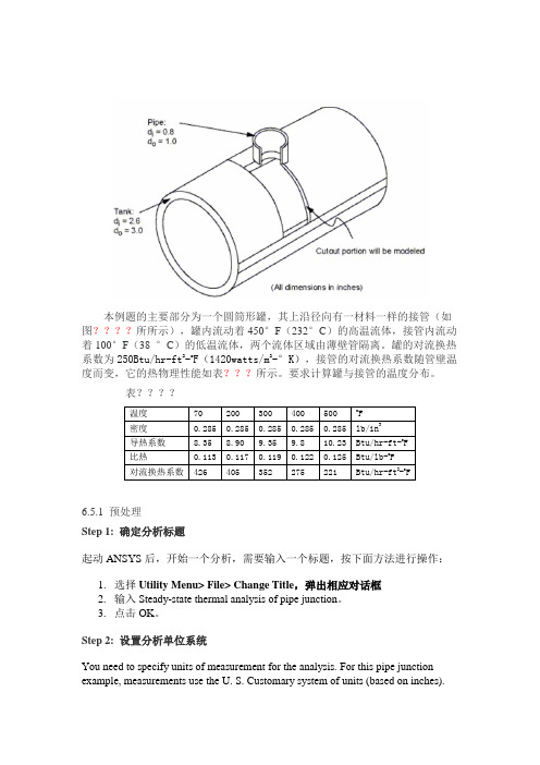
本例题的主要部分为一个圆筒形罐,其上沿径向有一材料一样的接管(如图????所所示),罐内流动着450°F(232°C)的高温流体,接管内流动着100°F(38 °C)的低温流体,两个流体区域由薄壁管隔离。
罐的对流换热系数为250Btu/hr-ft2-o F(1420watts/m2-°K),接管的对流换热系数随管壁温度而变,它的热物理性能如表???所示。
要求计算罐与接管的温度分布。
表????6.5.1 预处理Step 1: 确定分析标题起动ANSYS后,开始一个分析,需要输入一个标题,按下面方法进行操作:1.选择Utility Menu> File> Change Title,弹出相应对话框2.输入 Steady-state thermal analysis of pipe junction。
3.点击OK。
Step 2: 设置分析单位系统You need to specify units of measurement for the analysis. For this pipe junction example, measurements use the U. S. Customary system of units (based on inches).To specify this, type the command /UNITS,BIN in the ANSYS Input window and press ENTER.在分析之前,需要为分析系统设定单位系统,Step 3: Define the Element TypeThe example analysis uses a thermal solid element. To define it, do the following:1.Choose Main Menu> Preprocessor> Element Type> Add/Edit/Delete. TheElement Types dialog box appears.2.Click on Add. The Library of Element Types dialog box appears.3.In the list on the left, scroll down and pick (highlight) "Thermal Solid." In thelist on the right, pick "Brick20node 90."4.Click on OK.5.Click on Close to close the Element Types dialog box.Step 4: Define Material PropertiesTo define material properties for the analysis, perform these steps:1.Choose Main Menu> Preprocessor> Material Props> Material Models.The Define Material Model Behavior dialog box appears.2.In the Material Models Available window, double-click on the followingoptions: Thermal, Density. A dialog box appears.3.Enter .285 for DENS (Density), and click on OK. Material Model Number 1appears in the Material Models Defined window on the left.4.In the Material Models Available window, double-click on the followingoptions: Conductivity, Isotropic. A dialog box appears.5.Click on the Add Temperature button four times. Four columns are added.6.In the T1 through T5 fields, enter the following temperature values: 70, 200,300, 400, and 500. Select the row of temperatures by dragging the cursoracross the text fields. Then copy the temperatures by pressing Ctrl-c.7.In the KXX (Thermal Conductivity) fields, enter the following values, in order,for each of the temperatures, then click on OK. Note that to keep the unitsconsistent, each of the given values of KXX must be divided by 12. You canjust input the fractions and have ANSYS perform the calculations.8.35/128.90/129.35/129.80/1210.23/128.In the Material Models Available window, double-click on Specific Heat. Adialog box appears.9.Click on the Add Temperature button four times. Four columns are added.10.With the cursor positioned in the T1 field, paste the five temperatures bypressing Ctrl-v.11.In the C (Specific Heat) fields, enter the following values, in order, for each ofthe temperatures, then click on OK..113.117.119.122.12512.Choose menu path Material> New Model, then enter 2 for the new MaterialID. Click on OK. Material Model Number 2 appears in the Material ModelsDefined window on the left.13.In the Material Models Available window, double-click on Convection orFilm Coef. A dialog box appears.14.Click on the Add Temperature button four times. Four columns are added.15.With the cursor positioned in the T1 field, paste the five temperatures bypressing Ctrl-v.16.In the HF (Film Coefficient) fields, enter the following values, in order, foreach of the temperatures. To keep the units consistent, each value of HF must be divided by 144. As in step 7, you can input the data as fractions and letANSYS perform the calculations.426/144405/144352/144275/144221/14417.Click on the Graph button to view a graph of Film Coefficients vs.temperature, then click on OK.18.Choose menu path Material> Exit to remove the Define Material ModelBehavior dialog box.19.Click on SAVE_DB on the ANSYS Toolbar.Step 5: Define Parameters for Modeling1.Choose Utility Menu> Parameters> Scalar Parameters. The ScalarParameters window appears.2.In the window's Selection field, enter the values shown below. (Do not enterthe text in parentheses.) Press ENTER after typing in each value. If you makea mistake, simply retype the line containing the error.RI1=1.3 (Inside radius of the cylindrical tank)RO1=1.5 (Outside radius of the tank)Z1=2 (Length of the tank)RI2=.4 (Inside radius of the pipe)RO2=.5 (Outside radius of the pipe)Z2=2 (Length of the pipe)3.Click on Close to close the window.Step 6: Create the Tank and Pipe Geometry1.Choose Main Menu> Preprocessor> Modeling> Create> Volumes>Cylinder> By Dimensions. The Create Cylinder by Dimensions dialog boxappears.2.Set the "Outer radius" field to RO1, the "Optional inner radius" field to RI1,the "Z coordinates" fields to 0 and Z1 respectively, and the "Ending angle"field to 90.3.Click on OK.4.Choose Utility Menu>WorkPlane> Offset WP by Increments. The OffsetWP dialog box appears.5.Set the "XY, YZ, ZX Angles" field to 0,-90.6.Click on OK.7.Choose Main Menu> Preprocessor> Modeling> Create> Volumes>Cylinder> By Dimensions. The Create Cylinder by Dimensions dialog boxappears.8.Set the "Outer radius" field to RO2, the "Optional inner radius" field to RI2,the "Z coordinates" fields to 0 and Z2 respectively. Set the "Starting angle"field to -90 and the "Ending Angle" to 0.9.Click on OK.10.Choose Utility Menu>WorkPlane> Align WP with> Global Cartesian. Step 7: Overlap the Cylinders1.Choose Main Menu> Preprocessor> Modeling> Operate> Booleans>Overlap> Volumes. The Overlap Volumes picking menu appears.2.Click on Pick All.Step 8: Review the Resulting ModelBefore you continue with the analysis, quickly review your model. To do so, follow these steps:1.Choose Utility Menu>PlotCtrls> Numbering. The Plot Numbering Controlsdialog box appears.2.Click the Volume numbers radio button to On, then click on OK.3.Choose Utility Menu>PlotCtrls> View Settings> Viewing Direction. Adialog box appears.4.Set the "Coords of view point" fields to (-3,-1,1), then click on OK.5.Review the resulting model.6.Click on SAVE_DB on the ANSYS Toolbar.Step 9: Trim Off Excess VolumesIn this step, delete the overlapping edges of the tank and the lower portion of the pipe.1.Choose Main Menu> Preprocessor> Modeling> Delete> Volume andBelow. The Delete Volume and Below picking menu appears.2.In the picking menu, type 3,4 and press the ENTER key. Then click on OK inthe Delete Volume and Below picking menu.Step 10: Create Component AREMOTEIn this step, you select the areas at the remote Y and Z edges of the tank and save them as a component called AREMOTE. To do so, perform these tasks:1.Choose Utility Menu> Select> Entities. The Select Entities dialog boxappears.2.In the top drop down menu, select Areas. In the second drop down menu,select By Location. Click on the Z Coordinates radio button.3.Set the "Min,Max" field to Z1.4.Click on Apply.5.Click on the Y Coordinates and Also Sele radio buttons.6.Set the "Min,Max" field to 0.7.Click on OK.8.Choose Utility Menu> Select> Comp/Assembly> Create Component. TheCreate Component dialog box appears.9.Set the "Component name" field to AREMOTE. In the "Component is madeof" menu, select Areas.10.Click on OK.Step 11: Overlay Lines on Top of AreasDo the following:1.Choose Utility Menu>PlotCtrls> Numbering. The Plot Numbering Controlsdialog box appears.2.Click the Area and Line number radio boxes to On and click on OK.3.Choose Utility Menu> Plot> Areas.4.Choose Utility Menu>PlotCtrls> Erase Options.5.Set "Erase between Plots" radio button to Off.6.Choose Utility Menu> Plot> Lines.7.Choose Utility Menu>PlotCtrls> Erase Options.8.Set "Erase between Plots" radio button to On.Step 12: Concatenate Areas and LinesIn this step, you concatenate areas and lines at the remote edges of the tank for mapped meshing. To do so, follow these steps:1.Choose Main Menu> Preprocessor> Meshing> Mesh> Volumes> Mapped>Concatenate> Areas. The Concatenate Areas picking menu appears.2.Click on Pick All.3.Choose Main Menu> Preprocessor> Meshing> Mesh> Volumes> Mapped>Concatenate> Lines. A picking menu appears.4.Pick (click on) lines 12 and 7 (or enter in the picker).5.Click on Apply.6.Pick lines 10 and 5 (or enter in picker).7.Click on OK.Step 13: Set Meshing Density Along Lines1.Choose Main Menu> Preprocessor> Meshing> SizeCntrls>ManualSize>Lines> Picked Lines. The Element Size on PickedLines picking menu appears.2.Pick lines 6 and 20 (or enter in the picker) .3.Click on OK. The Element Sizes on Picked Lines dialog box appears.4.Set the "No. of element divisions" field to 4.5.Click on OK.6.Choose Main Menu> Preprocessor> Meshing> Size Cntrls>ManualSize>Lines> Picked Lines. A picking menu appears.7.Pick line 40 (or enter in the picker).8.Click on OK. The Element Sizes on Picked Lines dialog box appears.9.Set the "No. of element divisions" field to 6.10.Click on OK.Step 14: Mesh the ModelIn this sequence of steps, you set the global element size, set mapped meshing, then mesh the volumes.1.Choose Utility Menu> Select> Everything.2.Choose Main Menu> Preprocessor> Meshing> Size Cntrls>ManualSize>Global> Size. The Global Element Sizes dialog box appears.3.Set the "Element edge length" field to 0.4 and click on OK.4.Choose Main Menu> Preprocessor> Meshing>Mesher Opts. The MesherOptions dialog box appears.5.Set the Mesher Type radio button to Mapped and click on OK. The SetElement Shape dialog box appears.6.In the 2-D shape key drop down menu, select Quad and click on OK.7.Click on the SAVE_DB button on the Toolbar.8.Choose Main Menu> Preprocessor> Meshing> Mesh> Volumes> Mapped>4 to 6 sided. The Mesh Volumes picking menu appears. Click on Pick All. Inthe Graphics window, ANSYS builds the meshed model. If a shape testingwarning message appears, review it and click Close.Step 15: Turn Off Numbering and Display Elements1.Choose Utility Menu>PlotCtrls> Numbering. The Plot Numbering Controlsdialog box appears.2.Set the Line, Area, and Volume numbering radio buttons to Off.3.Click on OK.Step 16: Define the Solution Type and OptionsIn this step, you tell ANSYS that you want a steady-state solution that uses a program-chosen Newton-Raphson option.1.Choose Main Menu> Solution> Analysis Type> New Analysis. The NewAnalysis dialog box appears.2.Click on OK to choose the default analysis type (Steady-state).3.Choose Main Menu> Solution> Analysis Type> Analysis Options. TheStatic or Steady-State dialog box appears.4.Click on OK to accept the default (“Program-chosen”) for "Newton-Raphsonoption."Step 17: Set Uniform Starting TemperatureIn a thermal analysis, set a starting temperature.1.Choose Main Menu> Solution> Define Loads> Apply> Thermal>Temperature> Uniform Temp. A dialog box appears.2.Enter 450 for "Uniform temperature." Click on OK.Step 18: Apply Convection LoadsThis step applies convection loads to the nodes on the inner surface of the tank.1.Choose Utility Menu>WorkPlane> Change Active CS to> GlobalCylindrical.2.Choose Utility Menu> Select> Entities. The Select Entities dialog boxappears.3.Select Nodes and By Location, and click on the X Coordinates and From Fullradio buttons.4.Set the "Min,Max" field to RI1 and click on OK.5.Choose Main Menu> Solution> Define Loads> Apply> Thermal>Convection> On Nodes. The Apply CONV on Nodes picking menu appears.6.Click on Pick All. The Apply CONV on Nodes dialog box appears.7.Set the "Film coefficient" field to 250/144.8.Set the "Bulk temperature" field to 450.9.Click on OK.Step 19: Apply Temperature Constraints to AREMOTE Component1.Choose Utility Menu> Select> Comp/Assembly> Select Comp/Assembly.A dialog box appears.2.Click on OK to select component AREMOTE.3.Choose Utility Menu> Select> Entities. The Select Entities dialog boxappears.4.Select Nodes and Attached To, and click on the Areas,All radio button. Clickon OK.5.Choose Main Menu> Solution> Define Loads> Apply> Thermal>Temperature> On Nodes. The Apply TEMP on Nodes picking menuappears.6.Click on Pick All. A dialog box appears.7.Set the "Load TEMP value" field to 450.8.Click on OK.9.Click on SAVE_DB on the ANSYS Toolbar.Step 20: Apply Temperature-Dependent ConvectionIn this step, apply a temperature-dependent convection load on the inner surface of the pipe.1.Choose Utility Menu>WorkPlane> Offset WP by Increments. A dialog boxappears.2.Set the "XY,YZ,ZX Angles" field to 0,-90, then click on OK.3.Choose Utility Menu>WorkPlane> Local Coordinate Systems> CreateLocal CS> At WP Origin. The Create Local CS at WP Origin dialog boxappears.4.On the "Type of coordinate system" menu, select "Cylindrical 1" and click onOK.5.Choose Utility Menu> Select> Entities. The Select Entities dialog boxappears.6.Select Nodes, and By Location, and click on the X Coordinates radio button.7.Set the "Min,Max" field to RI2.8.Click on OK.9.Choose Main Menu> Solution> Define Loads> Apply> Thermal>Convection> On Nodes. The Apply CONV on Nodes picking menu appears.10.Click on Pick All. A dialog box appears.11.Set the "Film coefficient" field to -2.12.Set the "Bulk temperature" field to 100.13.Click on OK.14.Choose Utility Menu> Select> Everything.15.Choose Utility Menu>PlotCtrls> Symbols. The Symbols dialog box appears.16.On the "Show pres and convect as" menu, select Arrows, then click on OK.17.Choose Utility Menu> Plot> Nodes. The display in the Graphics Windowchanges to show you a plot of nodes.Step 21: Reset the Working Plane and Coordinates1.To reset the working plane and default Cartesian coordinate system,choose Utility Menu>WorkPlane> Change Active CS to> GlobalCartesian.2.Choose Utility Menu>WorkPlane> Align WP With> Global Cartesian. Step 22: Set Load Step OptionsFor this example analysis, you need to specify 50 substeps with automatic time stepping.1.Choose Main Menu> Solution> Load Step Options> Time/Frequenc>Time and Substps. The Time and Substep Options dialog box appears.2.Set the "Number of substeps" field to 50.3.Set "Automatic time stepping" radio button to On.4.Click on OK.Step 23: Solve the Model1.Choose Main Menu> Solution> Solve> Current LS. The ANSYS programdisplays a summary of the solution options in a /STAT command window.2.Review the summary.3.Choose Close to close the /STAT command window.4.Click on OK in the Solve Current Load Step dialog box.5.Click Yes in the Verify message window.6.The solution runs. When the Solution is done! window appears, click onClose.Step 24: Review the Nodal Temperature Results1.Choose Utility Menu>PlotCtrls> Style> Edge Options. The Edge Optionsdialog box appears.2.Set the "Element outlines" field to "Edge only" for contour plots and click onOK.3.Choose Main Menu> General Postproc> Plot Results> Contour Plot>Nodal Solu. The Contour Nodal Solution Data dialog box appears.4.For "Item to be contoured," pick "DOF solution" from the list on the left, thenpick "Temperature TEMP" from the list on the right.5.Click on OK. The Graphics window displays a contour plot of the temperatureresults.Step 25: Plot Thermal Flux VectorsIn this step, you plot the thermal flux vectors at the intersection of the pipe and tank.1.Choose Utility Menu>WorkPlane> Change Active CS to> Specified CoordSys. A dialog box appears.2.Set the "Coordinate system number" field to 11.3.Click on OK.4.Choose Utility Menu> Select> Entities. The Select Entities dialog boxappears.5.Select Nodes and By Location, and click the X Coordinates radio button.6.Set the "Min,Max" field to RO2.7.Click on Apply.8.Select Elements and Attached To, and click the Nodes radio button.9.Click on Apply.10.Select Nodes and Attached To, then click on OK.11.Choose Main Menu> General Postproc> Plot Results> Vector Plot>Predefined. A dialog box appears.12.For "Vector item to be plotted," choose "Flux & gradient" from the list on theleft and choose "Thermal flux TF" from the list on the right.13.Click on OK. The Graphics Window displays a plot of thermal flux vectors. Step 26: Exit from ANSYSTo leave the ANSYS program, click on the QUIT button in the Toolbar. Choose an exit option and click on OK.。
ANSYS稳态和瞬态分析步骤简述..
ANSYS 稳态和瞬态热模拟基本步骤基于ANSYS 9.0一、 稳态分析从温度场是否是时间的函数即是否随时间变化上,热分析包括稳态和瞬态热分析。
其中,稳态指的是系统的温度场不随时间变化,系统的净热流率为0,即流入系统的热量加上系统自身产生的热量等于流出系统的热量:=0q q q +-流入生成流出 在稳态分析中,任一节点的温度不随时间变化。
基本步骤:(为简单起见,按照软件的菜单逐级介绍)1、 选择分析类型点击Preferences 菜单,出现对话框1。
对话框1我们主要针对的是热分析的模拟,所以选择Thermal 。
这样做的目的是为了使后面的菜单中只有热分析相关的选项。
2、 定义单元类型GUI :Preprocessor>Element Type>Add/Edit/Delete 出现对话框2对话框2(3-1)点击Add,出现对话框3对话框3在ANSYS中能够用来热分析的单元大约有40种,根据所建立的模型选择合适的热分析单元。
对于三维模型,多选择SLOID87:六节点四面体单元。
3、选择温度单位默认一般都是国际单位制,温度为开尔文(K)。
如要改为℃,如下操作GUI:Preprocessor>Material Props>Temperature Units选择需要的温度单位。
4、定义材料属性对于稳态分析,一般只需要定义导热系数,他可以是恒定的,也可以随温度变化。
GUI: Preprocessor>Material Props> Material Models 出现对话框4对话框4一般热分析,材料的热导率都是各向同性的,热导率设定如对话框5.对话框5若要设定材料的热导率随温度变化,主要针对半导体材料。
则需要点击对话框5中的Add Temperature选项,设置不同温度点对应的热导率,当然温度点越多,模拟结果越准确。
设置完毕后,可以点击Graph按钮,软件会生成热导率随温度变化的曲线。
- 1、下载文档前请自行甄别文档内容的完整性,平台不提供额外的编辑、内容补充、找答案等附加服务。
- 2、"仅部分预览"的文档,不可在线预览部分如存在完整性等问题,可反馈申请退款(可完整预览的文档不适用该条件!)。
- 3、如文档侵犯您的权益,请联系客服反馈,我们会尽快为您处理(人工客服工作时间:9:00-18:30)。
【问题描述】
一个保温桶,由4层组成。
从外到内依次是:钢,铝,复合材料,铝。
桶内是热水,而桶外是空气。
需要确定桶壁的温度场分布。
已知:桶内半径是0.1米,桶长度为0.1米,从内到外,4层厚度分别是0.01米,0.02米,0.01米,0.005米,钢,复合材料,铝的导热系数分别是60.5(瓦/米度),0.055(瓦/米度),236(瓦/米度),水温80摄氏度,空气温度为摄氏度,空气对流系数是12.5(瓦/平方米度).
(《注》该例子来自于许京荆编著的《ANSYS 13.0 WORKBENCH数值模拟技术》,2012年)
【建模分析】
1.这是一个稳态热分析问题,需要使用steady-state thermal模块。
2. 这是一个轴对称问题,只需要分析其一个径向截面,然后用2D分析的轴对称进行处理。
3.几何建模。
在DM中创建四个草图,然后分别形成四个面体,再形成一个多体构件。
4.边界条件。
对里层使用温度边界条件,对外层设置对流换热边界条件。
【求解过程】
1. 打开ANSYS WORKBNCH14.5。
2. 创建稳态热分析系统。
3. 设置三种材料的导热系数。
双击engineering data,打开工程数据,新创建三种材料,分别是STEEL,AL,compound,并分别设置其导热系数。
钢材的导热系数
铝的导热系数
复合材料的导热系数
创建完毕,退回到项目中。
4.创建几何模型。
双击geometry,进入到DM中。
选择长度的单位是米。
在XOY面内创建四个草图。
这四个草图是四个相邻的矩形,其位置及尺寸如下图。
分别由这4个草图生成4个面。
其图形如下
将上述四个物体生成一个多体构件。
几何建模结束,存盘,退出DM.
然后设置几何体的属性是2D,表明下面准备做的是2D分析。
5.为各几何体分配材料。
双击model,进入到mechanical.
首先选中geometry,在其属性栏中设置是做轴对称分析。
然后为各个几何4体分配材料。
6.划分网格。
进行映射网格划分。
考察网格质量
可见,网格质量良好。
7.设置边界条件。
设置内层温度为80度,即热水的温度。
设置外层为对流换热。
环境温度20度,对流换热系数是12.5.
8.求解。
9.后处理。
查看温度的分布
可见,在最里层及外面的两层,温度基本上均匀分布,而在复合材料层,则温度从内到外逐渐降低。
由于该层是复合材料层,导热系数很小,所以阻碍了热量的传递,而此层的温度梯度最大。
查看总的热通量
可见,热通量由内向外逐步减少。