用STATA做空间计量
【最新】空间计量代码
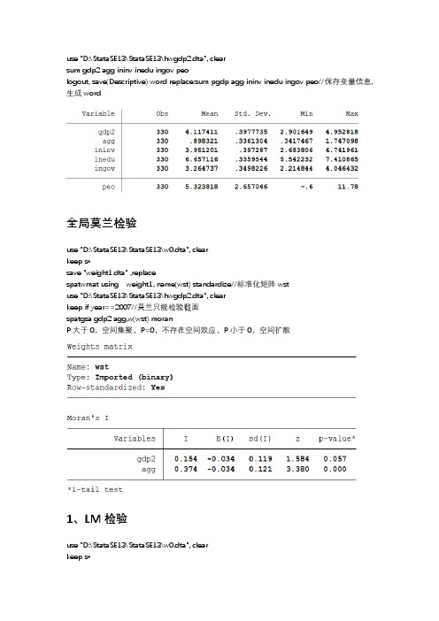
use "D:\StataSE13\StataSE13\hwgdp2.dta", clearsum gdp2 agg ininv inedu ingov peologout, save(Descriptive) word replace:sum pgdp agg ininv inedu ingov peo//保存变量信息,生成word全局莫兰检验use "D:\StataSE13\StataSE13\w0.dta", clearkeep s*save "weight1.dta" ,replacespatwmat using weight1, name(wst) standardize//标准化矩阵wstuse "D:\StataSE13\StataSE13\hwgdp2.dta", clearkeep if year==2007//莫兰只能检验截面spatgsa gdp2 agg,w(wst) moranP大于0,空间集聚,P=0,不存在空间效应,P小于0,空间扩散1、LM检验use "D:\StataSE13\StataSE13\w0.dta", clearkeep s*save "weight1.dta" ,replacespatwmat using weight1, name(wst) standardizeuse "D:\StataSE13\StataSE13\hwgdp2.dta", clearxtset id yearspwmatrix import using weight1.dta,wname(w6) dta xtw(11)qui reg gdp2 agg ininv inedu ingov peo//一般面板回归,但是不显示spatdiag,weights(w6)P=0,接受空间误差P≠0,拒绝空间滞后2、LR检验本文只检验SEM和SDMqui xsmle gdp2 agg ininv inedu ingov peo, wmat(wst) model(sdm) fe type(ind) nsim(500) nolog effectsestest store sdmqui xsmle gdp2 agg ininv inedu ingov peo , emat(wst) model(sem) fe type(ind) nsim(500) nolog effectsestest store semlrtest sdm semP=0,选择杜宾3、Hausman检验qui xsmle gdp2 agg ininv inedu ingov peo, wmat(wst) model(sdm) fe type(ind) nsim(500) nolog effectsest.est sto fequi xsmle gdp2 agg ininv inedu ingov peo, wmat(wst) model(sdm) re type(ind) nsim(500) nolog effectsestest sto re负数,则个体固定效应,故用fe。
【计量】空间杜宾模型代码
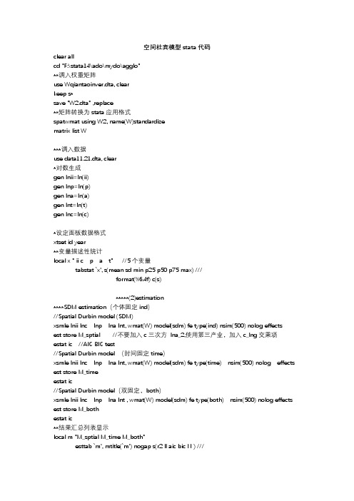
空间杜宾模型stata代码clear allcd "F:\stata14\ado\mydo\agglo"**调入权重矩阵use Wqiantaoinver.dta, clearkeep s*save "W2.dta" ,replace**矩阵转换为stata应用格式spatwmat using W2, name(W)standardizematrix list W***调入数据use data11.21.dta, clear*对数生成gen lnii=ln(ii)gen lnp=ln(p)gen lna=ln(a)gen lnt=ln(t)gen lnc=ln(c)*设定面板数据格式xtset id year**变量描述性统计local x " ii c p a t" //5个变量tabstat `x', s(mean sd min p25 p50 p75 max) ///format(%6.4f) c(s)*****(2)estimation****SDM estimation(个体固定ind)//Spatial Durbin model (SDM)xsmle lnii lnc lnp lna lnt, wmat(W) model(sdm) fe type(ind) nsim(500) nolog effectsest store M_sptial //不要加入c三次方lna_2,使用第三产业,加入c_lng交乘项estat ic //AIC BIC test//Spatial Durbin model (时间固定time)xsmle lnii lnc lnp lna lnt, wmat(W) model(sdm) fe type(time) nsim(500) nolog effects est store M_timeestat ic//Spatial Durbin model(双固定,both)xsmle lnii lnc lnp lna lnt , wmat(W) model(sdm) fe type(both) nsim(500) nolog effects est store M_bothestat ic**结果汇总列表显示local m "M_sptial M_time M_both"esttab `m', mtitle(`m') nogap s(r2 ll aic bic N ) ///star(* 0.1 ** 0.05 *** 0.01) b(%6.3f)esttab M_sptial M_time M_both using pane0000.rtf //输出结果rtf excel doc****hausman testxsmle lnii lnc lnp lna lnt , wmat(W) model(sdm) fe type(both) nsim(500) nolog estimates store sdm_fexsmle lnii lnc lnp lna lnt , wmat(W) model(sdm) re type(both) nsim(500) nolog estimates store sdm_rehausman sdm_fe sdm_re。
截面空间计量stata代码
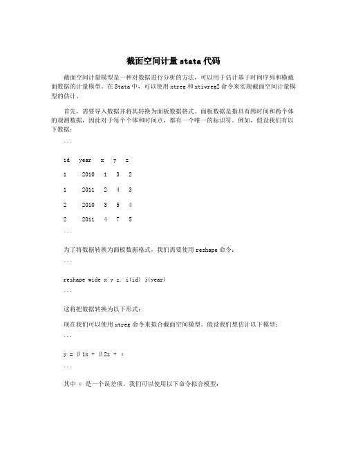
截面空间计量stata代码截面空间计量模型是一种对数据进行分析的方法,可以用于估计基于时间序列和横截面数据的计量模型。
在Stata中,可以使用xtreg和xtivreg2命令来实现截面空间计量模型的估计。
首先,需要导入数据并将其转换为面板数据格式。
面板数据是指具有跨时间和跨个体的观测数据,因此对于每个个体和时间点,都有一个唯一的标识符。
例如,假设我们有以下数据:```id year x y z1 2010 1 3 21 20112 4 32 20103 5 42 2011 4 7 5```为了将数据转换为面板数据格式,我们需要使用reshape命令:```reshape wide x y z, i(id) j(year)```这将把数据转换为以下形式:现在我们可以使用xtreg命令来拟合截面空间模型。
假设我们想估计以下模型:```y = β1x + β2z + ε```其中ε是一个误差项。
我们可以使用以下命令拟合模型:这将估计固定效应模型,其中id被视为固定效应,表示个体之间的差异。
如果我们希望估计随机效应模型,可以使用以下命令:如果我们希望进行仪器变量回归(IV回归),可以使用xtivreg2命令。
假设我们的模型是以下形式:这将估计固定效应模型,并使用z作为仪器变量来消除x的内生性问题。
在估计截面空间模型时,还可以使用其他选项来指定模型的特征,例如使用聚类标准误来对标准误进行调整,使用robust选项来进行鲁棒性检验,使用vce(cluster id)来进行群集稳健性检验等。
面板空间计量之Stata应用

面板空间计量之Stata应用:学习笔记【同舟共济】更新于2016年4月20日说明目前,在空间计量方面,Stata官方命令语句数量有限且较为零散,尚未形成系统的空间计量工具包。
因此,个人建议空间计量的初学者转向Matlab软件,James P. LeSage、J. P. Elhorst、Donald J. Lacombe等学者所开发的空间计量工具包,其功能相对更加完善,操作起来也比较方便。
本人已经习惯了使用stata,初次自学空间计量方面的操作,参考help文件及相关文献,在学习过程中做了简要总结,仅供初学者交流学习。
其中若有不当之处,敬请批评指正,谢谢!E-mail: ares0825@【Stata】Abd Elmessih Shehata (Econpapers)URL: /RAS/psh494.htmFederico Belotti (Econpapers)URL: /RAS/pbe427.htmP. Wilner Jeanty (Econpapers)URL:/RAS/pje95.htmMaurizio PisatiURL:/people/maurizio-pisatiYihua Yu (Econpapers)URL:/RAS/pyu79.htm目录第一章Stata空间计量命令语句安装 1 第二章中国31省市自治区(不含港澳台、附属岛屿)shp制作 3 第三章Stata空间权重制作8 第四章Stata 空间相关性检验27 第五章Stata 空间面板数据回归39面板空间计量之Stata应用:学习笔记第一章Stata空间计量命令包安装更新于2016-03-151.空间计量-Stata命令包Archive of user-written Stata packagesURL: /statistics/stata-blog/stata-programming/ssc_stata_package_list.php图1 Stata用户自拟命令语句列表另外,在IDEAS(URL: https:///)中可以查询相关命令,顺便推荐几个论坛,大家可以经常逛逛:Stata官方论坛URL: /UCLA-Idre论坛URL: /stat/stata/Stata Daily URL: /index/2.安装单击图1左侧红色框内命令名称,即可下载对应的压缩包,安装过程参考非官方命令手动安装说明(URL:/thread-2420580-1-1.html);单击图1右侧蓝色框内的各命令所对应的描述性语句,即可看到该命令的详细说明及应用举例。
空间计量莫兰指数 stata

空间计量莫兰指数 stata空间计量莫兰指数是基于莫兰散点图(Moran Scatterplot)提出的。
莫兰散点图是一种用来可视化空间相关性的图形工具,它将地理现象的值与其周围邻居的均值进行比较,从而揭示地理现象的空间分布特征。
空间计量莫兰指数则是在莫兰散点图的基础上进行数值化的指标,它可以给出一个介于-1和1之间的值,用来描述地理现象的空间相关性程度。
在 Stata 中计算空间计量莫兰指数需要使用 spatwmat 命令来构建空间权重矩阵,然后使用spmoran 命令来计算莫兰指数及其统计显著性。
首先,我们需要准备一份包含地理现象值和空间位置信息的数据集。
然后,可以使用spatwmat 命令根据空间邻居关系构建空间权重矩阵。
空间权重矩阵定义了每个地理现象值与其邻居之间的关系强度,常用的权重定义方法包括距离权重和邻近权重。
构建好空间权重矩阵后,可以使用spmoran 命令来计算莫兰指数及其统计显著性。
在解释空间计量莫兰指数时,一般需要关注两个方面的信息。
首先是莫兰指数的数值,它可以告诉我们地理现象的空间相关性程度。
当莫兰指数接近1时,表示地理现象存在正相关性,即相似的值聚集在一起;当莫兰指数接近-1时,表示地理现象存在负相关性,即相异的值聚集在一起;当莫兰指数接近0时,表示地理现象不存在空间相关性。
其次是莫兰指数的显著性,它可以告诉我们莫兰指数是否具有统计意义。
一般来说,当莫兰指数的显著性水平小于0.05时,可以认为地理现象存在显著的空间相关性。
为了更好地理解空间计量莫兰指数的应用,我们以某市的犯罪率数据为例进行分析。
首先,我们需要准备一份包含犯罪率和地理位置信息的数据集。
然后,可以使用spatwmat 命令构建空间权重矩阵,以考虑犯罪率值之间的空间关系。
接下来,使用spmoran 命令计算莫兰指数及其显著性。
最后,可以通过莫兰散点图来可视化犯罪率的空间分布特征,并根据莫兰指数的数值和显著性来解释犯罪率的空间相关性。
空间计量模型stata代码
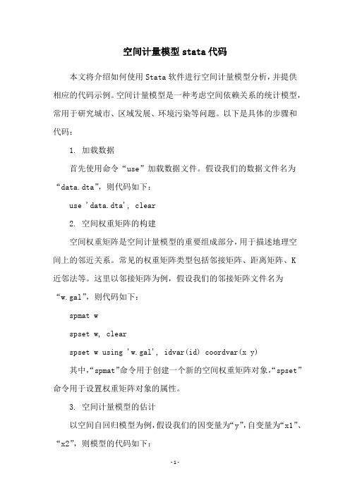
空间计量模型stata代码本文将介绍如何使用Stata软件进行空间计量模型分析,并提供相应的代码示例。
空间计量模型是一种考虑空间依赖关系的统计模型,常用于研究城市、区域发展、环境污染等问题。
以下是具体的步骤和代码:1. 加载数据首先使用命令“use”加载数据文件。
假设我们的数据文件名为“data.dta”,则代码如下:use 'data.dta', clear2. 空间权重矩阵的构建空间权重矩阵是空间计量模型的重要组成部分,用于描述地理空间上的邻近关系。
常见的权重矩阵类型包括邻接矩阵、距离矩阵、K近邻法等。
这里以邻接矩阵为例,假设我们的邻接矩阵文件名为“w.gal”,则代码如下:spmat wspset w, clearspset w using 'w.gal', idvar(id) coordvar(x y) 其中,“spmat”命令用于创建一个新的空间权重矩阵对象,“spset”命令用于设置权重矩阵对象的属性。
3. 空间计量模型的估计以空间自回归模型为例,假设我们的因变量为“y”,自变量为“x1”、“x2”,则模型的代码如下:spreg y x1 x2, wmatrix(w) robust其中,“spreg”命令用于进行空间自回归模型的估计,“wmatrix”选项用于指定权重矩阵对象,“robust”选项用于进行异方差性处理。
4. 结果输出和解释最后,使用“estimates”命令输出模型的估计结果,并进行解释。
例如,下面的代码将输出估计结果的标准误、t值和p值:estimates store model1estimates table model1, b(se) t(p) star(0.1 0.05 0.01) 其中,“estimates store”命令用于将估计结果存储到模型对象中,“estimates table”命令用于输出估计结果的表格形式。
解释结果时,需要注意权重矩阵的特征值和特征向量,以及空间自相关性的类型和程度。
Stata空间计量命令汇总及具体操作方法指南

Stata空间计量命令汇总及具体操作方法指南空间计量经济学创造性地处理了经典计量方法在面对空间数据时的缺陷,考察了数据在地理观测值之间的关联。
近年来在人文社会科学空间转向的大背景下,空间计量已成为空间综合人文学和社会科学研究的基础理论与方法,尤其在区域经济、房地产、环境、人口、旅游、地理、政治等领域,空间计量成为开展定量研究的必备技能。
1、空间计量建模步骤空间统计分析:构建空间权重矩阵后,进行探索性空间统计分析:包括空间相关性检验(全局空间自相关和局部空间自相关等);空间计量分析:空间计量模型的回归与检验(SAR,SEM,SAC 等模型估计和检验等)。
空间滞后模型(Spatial Lag Model,SLM)主要是探讨各变量在一地区是否有扩散现象(溢出效应)。
其模型表达式为:参数反映了自变量对因变量的影响,空间滞后因变量是一内生变量,反映了空间距离对区域行为的作用。
区域行为受到文化环境及与空间距离有关的迁移成本的影响,具有很强的地域性(Anselin et al.,1996)。
由于SLM模型与时间序列中自回归模型相类似,因此SLM也被称作空间自回归模型(Spatial Autoregressive Model,SAR)。
空间误差模型(Spatial Error Model,SEM)存在于扰动误差项之中的空间依赖作用,度量了邻近地区关于因变量的误差冲击对本地区观察值的影响程度。
由于SEM模型与时间序列中的序列相关问题类似,也被称为空间自相关模型(Spatial Autocorrelation Model,SAC)。
估计技术:鉴于空间回归模型由于自变量的内生性,对于上述两种模型的估计如果仍采用OLS,系数估计值会有偏或者无效,需要通过IV、ML或GLS、GMM等其他方法来进行估计。
Anselin (1988)建议采用极大似然法估计空间滞后模型(SLM)和空间误差模型(SEM)的参数。
空间自相关检验与SLM、SEM的选择:判断地区间创新产出行为的空间相关性是否存在,以及SLM和SEM那个模型更恰当,一般可通过包括Moran’s I检验、两个拉格朗日乘数(Lagrange Multiplier)形式LMERR、LMLAG及其稳健(Robust)的R-LMERR、R-LMLAG)等形式来实现。
利用STATA创建空间权重矩阵及空间杜宾模型计算----命令

** 创建空间权重矩阵介绍*设置默认路径cd C:\Users\xiubo\Desktop\F182013.v4\F101994\sheng**创建新文件*shp2dta:reads a shape (.shp) and dbase (.dbf) file from disk and converts them into Stata datasets.*shp2dta:读取CHN_adm1文件*CHN_adm1:为已有的地图文件*database (chinaprovince):表示创建一个名称为“chinaprovince”的dBase数据集*database(filename):Specifies filename of new dBase dataset*coordinates(coord):创建一个名称为“coord”的坐标系数据集*coordinates(filename):Specifies filename of new coordinates dataset*gencentroids(stub):Creates centroid variables*genid(newvarname):Creates unique id variable for database.dtashp2dta using CHN_adm1,database (chinaprovince) coordinates(coord) genid(id) gencentroids(c)**绘制2016年中國GDP分布圖*spmap:Visualization of spatial data*clnumber(#):number of classes*id(idvar):base map polygon identifier(识别符,声明变量名,一般以字母或下划线开头,包含数字、字母、下划线)*_2016GDP:变量*coord:之前创建的坐标系数据集spmap _2016GDP using coord, id(id) clnumber(5)*更改变量名rename x_c longituderename y_c latitude**生成距离矩阵*spmat:用于定义与管理空间权重矩阵*Spatial-weighting matrices are stored in spatial-weighting matrix objects (spmat objects).*spmat objects contain additional information about the data used in constructing spatial-weighting matrices.*spmat objects are used in fitting spatial models; see spreg (if installed) and spivreg (if installed).*idistance:(产生距离矩阵)create an spmat object containing an inverse-distance matrix W*或contiguity:create an spmat object containing a contiguity matrix W*idistance_jingdu:命名名称为“idistance_jingdu”的距離矩陣*longitude:使用经度*latitude:使用纬度*id(id):使用id*dfunction(function[, miles]):(设置计算距离方法)specify the distance function.*function may be one of euclidean (default), dhaversine, rhaversine, or the Minkowski distance of order p, where p is an integer greater than or equal to 1.*normalize(row):(行标准化)specifies one of the three available normalization techniques: row, minmax, and spectral.*In a row-normalized matrix, each element in row i is divided by the sum of row i's elements.*In a minmax-normalized matrix, each element is divided by the minimum of the largest row sum and column sum of the matrix.*In a spectral-normalized matrix, each element is divided by the modulus of the largest eigenvalue of the matrix.spmat idistance idistance_jingdu longitude latitude, id(id) dfunction(euclidean) normalize(row)**保存stata可读文件idistance_jingdu.spmatspmat save idistance_jingdu using idistance_jingdu.spmat**将刚刚保存的idistance_jingdu.spmat文件转化为txt文件spmat export idistance_jingdu using idistance_jingdu.txt**生成相邻矩阵spmat contiguity contiguity_jingdu using coord, id(id) normalize(row)spmat save contiguity_jingdu using contiguity_jingdu.spmatspmat export contiguity_jingdu using contiguity_jingdu.txt**计算Moran’s I*安装spatwmat*spatwmat:用于定义空间权重矩阵*spatwmat:imports or generates the spatial weights matrices required by spatgsa, spatlsa, spatdiag, and spatreg.*As an option, spatwmat also generates the eigenvalues matrix required by spatreg.*name(W):读取空间权重矩阵W*name(W):使用生成的空间权重矩阵W*xcoord:x坐标*ycoord:y坐标*band(0 8):宽窗介绍*band(numlist) is required if option using filename is not specified.*It specifies the lower and upper bounds of the distance band within which location pairs must be considered "neighbors" (i.e., spatially contiguous)*and, therefore, assigned a nonzero spatial weight.*binary:requests that a binary weights matrix be generated. To this aim, all nonzero spatial weights are set to 1.spatwmat, name(W) xcoord(longitude) ycoord(latitude) band(0 8)*安装绘制Moran’s I工具:splagvar*splagvar --- Generates spatially lagged variables, constructs the Moran scatter plot,*and calculates global Moran's I statistics.*_2016GDP:使用变量_2016GDP*wname(W):使用空间权重矩阵W*indicate the name of the spatial weights matrix to be used*wfrom(Stata):indicate source of the spatial weights matrix*wfrom(Stata | Mata) indicates whether the spatial weights matrix is a Stata matrix loaded in memory or a Mata file located in the working directory.*If the spatial weights matrix had been created using spwmatrix it should exist as a Stata matrix or as a Mata file.*moran(_2016GDP):计算变量_2016GDP的Moran's I值*plot(_2016GDP):构建变量_2016GDPMoran散点图splagvar _2016GDP, wname(W) wfrom(Stata) moran(_2016GDP) plot(_2016GDP)=============================================================================== **使用距离矩阵计算空间计量模型*设置默认路径cd D:\软件学习软件资料\stata\stata指导书籍命令\陈强高级计量经济学及stata应用(第二版)全部数据*使用product.dta数据集(陈强的高级计量经济学及其stata应用P594)*将数据集product.dta存入当前工作路径use product.dta , clear*创建新变量,对原有部分变量取对数gen lngsp=log(gsp)gen lnpcap=log(pcap)gen lnpc=log(pc)gen lnemp=log(emp)*将空间权重矩阵usaww.spat存入当前工作路径spmat use usaww using usaww.spmat*使用聚类稳健的标准误估计随机效应的SDM模型xsmle lngsp lnpcap lnpc lnemp unemp,wmat(usaww) model(sdm)robust nolog*使用选择项durbin(lnemp),不选择不显著的变量,使用聚类稳健的标准误估计随机效应的SDM模型xsmle lngsp lnpcap lnpc lnemp unemp,wmat(usaww) model(sdm) durbin(lnemp) robust nolog noeffects*使用选择项durbin(lnemp),不选择不显著的变量,使用聚类稳健的标准误估计固定效应的SDM模型xsmle lngsp lnpcap lnpc lnemp unemp,wmat(usaww) model(sdm) durbin(lnemp) robust nolog noeffects fe*存储随机效应和固定效应结果qui xsmle lngsp lnpcap lnpc lnemp unemp,wmat(usaww) model(sdm) durbin(lnemp) r2 nolog noeffects reest sto requi xsmle lngsp lnpcap lnpc lnemp unemp,wmat(usaww) model(sdm) durbin(lnemp) r2 nolog noeffects feest sto fe*esttab:将保存的结果汇总到一张表格中*b(fmt):specify format for point estimates*beta[(fmt)]:display beta coefficients instead of point est's*se[(fmt)]:display standard errors instead of t statistics*star( * 0.1 ** 0.05 *** 0.01):标记不同显著性水平对应的P值*r2|ar2|pr2[(fmt)]:display (adjusted, pseudo) R-squared*p[(fmt)]:display p-values instead of t statistics*label:make use of variable labels*title(string):specify a title for the tableesttab fe re , b se r2 star( * 0.1 ** 0.05 *** 0.01)*hausman检验*进行hausman检验前,回归中没有使用稳健标准误(没用“r”),*是因为传统的豪斯曼检验建立在同方差的前提下*constant:include estimated intercepts in comparison; default is to exclude*df(#):use # degrees of freedom*sigmamore:base both (co)variance matrices on disturbance variance estimate from efficient estimator*sigmaless:base both (co)variance matrices on disturbance variance estimate from consistent estimatorhausman fe re**有时我们还会得到负的chi2值,即chi2<0,表明模型不能满足Hausman检验的渐近假设。
空间计量莫兰指数 stata

空间计量莫兰指数 stata一、空间计量莫兰指数的概念空间计量莫兰指数是一种常用的空间自相关分析方法,用于研究地理空间上的数据分布是否存在空间相关性。
它通过计算空间单位之间的相似性来衡量空间数据的集聚程度,可以揭示出数据的空间分布特征和空间联系。
二、空间计量莫兰指数的计算方法空间计量莫兰指数的计算方法相对简单,可以使用Stata等统计软件进行计算。
首先,需要构建空间权重矩阵,它描述了空间单位之间的邻近关系。
常见的空间权重矩阵包括邻接矩阵和距离阈值矩阵。
然后,根据数据和空间权重矩阵,计算出莫兰指数的值。
莫兰指数的取值范围为-1到1,其中正值表示正相关,负值表示负相关,接近0表示无相关性。
三、空间计量莫兰指数的意义空间计量莫兰指数可以帮助我们理解地理空间上的数据分布规律和空间关联性。
通过分析莫兰指数,我们可以揭示出地理现象的空间集聚程度和空间联系的强弱程度。
这对于城市规划、区域发展、环境保护等领域的决策制定和问题解决具有重要意义。
四、空间计量莫兰指数的局限性空间计量莫兰指数作为一种统计分析方法,也存在一定的局限性。
首先,它只能揭示出数据之间的空间相关性,并不能说明因果关系。
其次,莫兰指数的计算依赖于空间权重矩阵的选择,不同的权重矩阵可能得到不同的结果。
此外,莫兰指数对样本量和数据分布的偏斜性也较为敏感,需要谨慎解释和使用。
空间计量莫兰指数是一种重要的空间自相关分析方法,可以帮助我们理解地理现象的空间分布特征和空间联系。
然而,我们在使用该指数进行分析时需要注意其局限性,结合具体问题和数据特点,谨慎解释和使用。
通过合理应用空间计量莫兰指数,我们可以更好地理解和解决与地理空间相关的问题,推动社会经济的可持续发展。
利用Stata命令进行空间杜宾模型分析
利用Stata命令进行空间杜宾模型分析标题:利用Stata命令进行空间杜宾模型分析介绍:在空间计量经济学领域,空间杜宾模型(Spatial Durbin Model)被广泛应用于探究空间依赖关系对经济现象的影响。
Stata作为一款常用的统计软件,提供了许多强大的命令来进行空间经济分析。
本文将介绍如何利用Stata命令进行空间杜宾模型的分析和解释。
一、概述空间杜宾模型是对传统杜宾模型的扩展,考虑了空间上的相互依赖关系。
其基本方程可以表示为:Y = ρWy + Xβ + λU + ε其中,Y是因变量,Wy表示空间邻近权重矩阵与因变量的乘积,X是自变量矩阵,β是参数向量,U是随机误差项,ε是空间误差项。
ρ和λ分别代表空间滞后和同时方程的空间依赖系数。
二、数据准备在Stata中进行空间杜宾模型的分析,首先要准备好需要的数据。
可以使用Stata的数据管理命令进行数据导入和转换,确保数据的一致性和准确性。
还需考虑到空间邻近权重矩阵的构建,可以使用Stata的空间数据分析命令来计算邻近矩阵。
三、模型估计利用Stata进行空间杜宾模型的估计,可以使用"splm"命令。
该命令提供了多种空间经济模型的估计方法,包括最小二乘法(OLS)、广义矩估计法(GMM)等。
在使用"splm"命令时,需要设定模型的形式和变量的选择。
四、模型诊断和解释为了确保模型的有效性和准确性,需要对模型进行诊断和解释。
可以通过Stata的模型诊断命令来进行一系列统计分析,如异方差性检验、空间误差的显著性检验等。
还可以使用Stata的模型解释命令来获取模型估计结果的解释,并进行进一步的分析和讨论。
五、实证案例分析在本节中,将以一个实证案例来展示如何使用Stata命令进行空间杜宾模型的分析。
案例数据为某地区的经济数据,包括GDP、人口、贸易等变量。
我们希望研究空间依赖对GDP的影响,并通过空间杜宾模型来分析这一关系。
计量经济学软件Stata15.0应用教程 课件 第九章 空间计量

hausman FE RE
( 1) 极大似然估计 spreg ml crime hoval income,id(id) dlm (A) elm (A) //MLE估计SARAR模型
( 2) 不含内生变量的gs2sls估计 spreg gs2sls crime hoval income, id(id) dlm (A) elm (A) het //GS2SLS估计SARAR模型 spreg gs2sls crime hoval income, id(id) dlm (A) het //不含空间误差的SAR模型 het(异方差 下的稳健标误)
spmat use B using usaww.spmat //用数据文件usaww.spmat生成空间权重矩阵B
SDM模型:
xsmle lngsp lnpcap lnpc lnemp unemp,wmat(B) model (sdm) r //随机效应估计 xsmle lngsp lnpcap lnpc lnemp unemp,wmat(B) model (sdm) durbin (lnemp) r //空间杜宾模型 xsmle lngsp lnpcap lnpc lnemp unemp,wmat(B) model (sdm) durbin (lnemp) r noeffe //固定效应 hausman检验:
空间计量模型stata代码

空间计量模型stata代码
空间计量模型stata代码是一种用于空间数据分析的统计软件,在stata中可以进行空间计量模型的建模和分析。
具体的代码包括以下几个步骤:
1.导入数据:使用stata命令“use”或者“import”导入需要分析的数据集。
2.定义空间权重矩阵:使用stata命令“spmat”或者“spwmatrix”定义空间权重矩阵,用于描述空间上的邻近关系。
3.空间回归模型建模:使用stata命令“spreg”或者“spatialreg”建立空间回归模型,其中包括空间滞后模型、空间错误模型、空间滞后误差模型等。
4.模型诊断和评价:使用stata命令“spatdiag”或者“sppack”对建立的空间回归模型进行诊断和评价,包括空间自相关性检验、异方差性检验、模型拟合度评价等。
5.结果分析和可视化:使用stata命令“spmap”或者“spgraph”对分析结果进行可视化展示,以便更好地理解和解释分析结果。
总之,空间计量模型stata代码是一种非常重要的工具,可以帮助研究者更好地理解和分析空间数据,并为相关领域的研究提供支持和帮助。
- 1 -。
stata空间计量计算空间矩阵乘自变量

stata空间计量计算空间矩阵乘自变量
本篇文章介绍如何在Stata软件中进行空间计量计算,重点是对空间矩阵乘自变量的操作。
首先需要了解何为空间计量,即考虑空间依赖性的变量之间的关系,这种依赖性通常表现为空间自相关性。
在进行空间计量分析时,需要将空间自相关性纳入模型中,使用空间权重矩阵来表示变量之间的空间联系。
然后,可以使用空间矩阵乘自变量的方法计算空间自相关性对模型的影响。
具体操作如下:
1. 准备空间权重矩阵:在Stata中,可以使用spatialweight 命令来生成空间权重矩阵,该命令可以根据不同的空间连接方式生成不同的权重矩阵,例如queen连接、rook连接等。
2. 载入数据:使用命令use读取数据文件。
3. 进行空间计量回归:使用命令spreg进行空间计量回归,将空间权重矩阵和自变量作为参数输入。
在进行回归分析时,可以使用OLS(ordinary least squares)或GM(generalized method of moments)方法,其中GM方法可以纠正空间自相关性引起的异方差性问题。
4. 计算空间矩阵乘自变量:使用命令spmatmul将空间权重矩阵乘以自变量,得到空间矩阵乘自变量的结果。
该结果可以用于分析空间自相关性对模型的影响,例如用于进行空间误差分解等。
总之,Stata软件提供了丰富的空间计量分析工具,可以方便
地进行空间矩阵乘自变量等计算操作,帮助研究者更好地理解空间
依赖性对变量关系的影响。
空间计量模型stata代码

空间计量模型stata代码很高兴为您提供关于空间计量模型的Stata代码,以下是详细的步骤和程序。
首先,您需要安装一些额外的包或插件。
安装STATA的-spcodes视察程序包:ssc install spcodes安装STATA的-spglmr回归建模程序包:ssc install spglmr在安装完这两个包之后,接下来就是编写代码。
以下是基于STATA的空间计量模型案例:sysuse cancer, clearspset lat long, fweight(pop)spreg cancer_rate income pct_access pct_access*pct_access, kernel(bisquare) bw(500000)lmtest注释:- 在这个案例中,我们使用了STATA的自带数据集“cancer”,这个数据集是关于美国的肺癌发病率等因素的一个非常有趣的数据集。
- 然后我们使用了spset lat long, fweight(pop)命令,指定了我们分析数据的经纬度和人口特征。
- 然后,我们使用了spreg cancer_rate income pct_accesspct_access*pct_access, kernel(bisquare) bw(500000)命令,指定了我们要分析的变量、核函数和带宽大小,具体解释如下:- cancer_rate是我们要预测的肺癌发病率变量;- income和pct_access是我们的解释变量,分别代表了所在地区的平均收入和公共交通设施的可获得度;- pct_access*pct_access表示我们在建模时使用了交互项;- kernel(bisquare)表示我们使用的核函数是双二次函数核函数; - bw(500000)表示我们选择了一个500km的带宽大小。
- 最后,我们使用了lmtest命令,对模型的有效性进行了测试。
运行上述代码后,您将获得一个关于空间计量模型的完整结果,包括模型参数估计的检验、误差项的统计以及模型预测的准确性等等。
重磅!Stata15的新模块(二):空间计量分析(续)

重磅!Stata15的新模块(二):空间计量分析(续)Prof. Lung-fei Lee (李龙飞)Ohio State University不久前,Stata 公司发布了最新的 Stata 15,包含了许多令人激动的重大升级,包括非参数回归、空间计量、门槛回归、DSGE 模型等。
本公众号将陆续为你介绍,与计量经济学最为相关的几个全新模块。
(接上期推文)初步检验空间效应在Stata 15 中定义好空间权重矩阵后,即可进行初步的空间效应检验。
基本方法就是,计算莫兰I 指数(Moran's I,本质上为空间自相关系数),然后考察其显著性。
为此,先进行 OLS 回归,比如:reg y x1 x2 x3其中,y 为被解释变量,x1,x2 与 x3 为解释变量。
然后,使用以下命令计算上述 OLS 回归残差的莫兰 I 指数,并检验其显著性。
estat moran, errorlag(W)其中,必选项errorlag(W) 用于指定空间权重矩阵(莫兰指数的定义依赖于空间权重矩阵),以检验残差(error)是否具有空间滞后(spatial lag)效应。
如果莫兰指数(空间自相关系数)显著不为 0,则说明存在空间效应,须进一步进行空间计量分析;反之,则或许没有必要。
在上述 OLS 回归中,也可以将自变量都去掉,只对常数项回归:reg yestat moran, errorlag(W)此时,就是检验被解释变量本身是否存在空间自相关(spatial autocorrelation)。
空间自回归模型空间计量的不少术语都源于时间序列。
比如,空间数据也称为“空间序列”(spatial series),即分布于空间的序列。
进一步,最常见的时间序列模型为自回归模型,比如AR(1),即依赖于它的一阶滞后(邻居)。
类似地,可以考虑空间序列的自回归模型(Spatial Autoregression,简记 SAR),即依赖于其一阶空间滞后(邻居)的(比如,某地区的犯罪率依赖于其相邻地区的犯罪率),可写为向量形式:其中,为的空间滞后(邻居),而参数即为空间自回归系数(spatial autoregressive coefficient),是空间计量分析首要感兴趣的参数;为扰动项。
空间计量经济学与Stata实现ppt课件

精品课件
• 在这种情况下,不同的权值指标随距离dij的定义而变化, 其取值取决于选定的函数形式(如距离的倒数或倒数的平 方,以及欧氏距离等)。
精品课件
空间权值矩阵的选择
• 尽管二进制的空间邻近权值矩阵并非适用于所有的空间计 量经济模型,但是,处于某些情况下的实用性,空间统计 学家在构建空间计量模型时的首选就是从二进制的邻近矩 阵开始的。
• 一般是先从空间邻近的最基本二进制矩阵开始,逐步选择 确定空间权值矩阵。
• 关于各种权值矩阵的选择,没有现成的理论根据,一般可 考虑空间计量模型对各种空间权值矩阵的适用程度,检验 估计结果对权值矩阵的敏感性,最终的依据实际上就是结 果的客观性和科学性。
• 正空间自相关:相似的观测值在空间集聚; • 负空间自相关:相似的观测值在空间分散; • 无空间自相关:观测值在空间分布上没有
规律(完全随机)。
精品课件
地区 Y y Y Y WA WB Wc WD WE
A 12 -9.1 0 1 1 1 0 B 15 -6.1 1 0 1 0 0 C 35 13.9 1 1 0 0 1 D 17 -4.1 1 0 0 0 1 E 28 6.93 0 0 1 1 0 F 20 -1.1 0 0 1 0 1
精品课件
二、空间自相关
空间权重矩阵
计量经济学经常用线性模型来近似非线性模型, 即可将
近似写成
记 矩阵 的元素为 元素都为零。
精品课件
,它的对角
空间自相关
用STATA做空间计量

How can I calculate Moran's I in Stata?Note: The commands shown in this page are user-written Stata commands that must be downloaded. To install the package of spatial analysis tools, type findit spatgsa in the command window.Moran's I is a measure of spatial autocorrelation--how related the values of a variable are based on the locations where they were measured. Using a set of user-written Stata commands, we can calculate Moran's I in Stata. We will be using the spatwmat command to generate a matrix of weights based on the locations in our data and the spatgsa command to calculate Moran's I or other spatial autocorrelation measures.Let's look at an example. Our dataset, ozone, contains ozone measurements from thirty-two locations in the Los Angeles area aggregated over one month. The dataset includes the station number (station), the latitude and longitude of the station (lat and lon), and the average of the highest eight hour daily averages (av8top). This data, and other spatial datasets, can be downloaded from the University of Illinois's Spatial Analysis Lab. We can look at a summary of our location variables to see the range of locations under consideration.use , clearsummarize lat lonV ariable | Obs Mean Std. Dev. Min Max-------------+--------------------------------------------------------lat | 32 34.0146 .2228168 33.6275 34.69012lon | 32 -117.7078 .5683853 -118.5347 -116.2339Based on the minimum and maximum values of these variables, we can calculate the greatest Euclidean distance we might measure between two points in our dataset.display sqrt((34.69012 - 33.6275)^2 + (-116.2339 - -118.5347)^2)2.5343326Knowing this maximum distance between two points in our data, we can generate a matrix based on the distances between points. In the spatwmat command, we name the weights matrix to be generated, indicate which of our variables are the x- and y-coordinate variables, and provide a range of distance values that are of interest in the band option. All of the distances are of interest in this example, so we create a band with an upper bound greater than our largest possible distance. If we did not care about distances greater than 2, we could indicate this in the band option.spatwmat, name(ozoneweights) xcoord(lon) ycoord(lat) band(0 3)The following matrix has been created:1. Inverse distance weights matrix ozoneweightsDimension: 32x32Distance band: 0 < d <= 3Friction parameter: 1Minimum distance: 0.11st quartile distance: 0.4Median distance: 0.63rd quartile distance: 1.0Maximum distance: 2.4Largest minimum distance: 0.50Smallest maximum distance: 1.23As described in the output, the command above generated a matrix with 32 rows and 32 columns because our data includes 32 locations. Each off-diagonal entry [i, j] in the matrix is equal to 1/(distance between point i and point j). Thus, the matrix entries for pairs of points that are close together are higher than for pairs of points that are far apart. If you wish to look at the matrix, you can display it with the matrix list command. With our matrix of weights, we can now calculate Moran's I.spatgsa av8top, weights(ozoneweights) moranMeasures of global spatial autocorrelationWeights matrix--------------------------------------------------------------Name: ozoneweightsType: Distance-based (inverse distance)Distance band: 0.0 < d <= 3.0Row-standardized: No--------------------------------------------------------------Moran's I--------------------------------------------------------------Variables | I E(I) sd(I) z p-value*--------------------+-----------------------------------------av8top | 0.248 -0.032 0.036 7.679 0.000--------------------------------------------------------------*1-tail testBased on these results, we can reject the null hypothesis that there is zero spatial autocorrelation present in the variable av8top at alpha = .05.VariationsBinary Matrix: If there exists some threshold distance d such that pairs with distances less than dare neighbors and pairs with distances greater than d are not, you can create a binary neighbors matrix with the spatwmat command (indicating bin and setting band to have an upper bound of d) and use this weights matrix for calculating Moran's I. We could do this for d = .75:spatwmat, name(ozoneweights) xcoord(lon) ycoord(lat) band(0 .75) binThe following matrix has been created:1. Distance-based binary weights matrix ozoneweightsDimension: 32x32Distance band: 0 < d <= .75Friction parameter: 1Minimum distance: 0.11st quartile distance: 0.4Median distance: 0.63rd quartile distance: 1.0Maximum distance: 2.4Largest minimum distance: 0.50Smallest maximum distance: 1.23spatgsa av8top, weights(ozoneweights) moranMeasures of global spatial autocorrelationWeights matrix--------------------------------------------------------------Name: ozoneweightsType: Distance-based (binary)Distance band: 0.0 < d <= 0.75Row-standardized: No--------------------------------------------------------------Moran's I--------------------------------------------------------------Variables | I E(I) sd(I) z p-value*--------------------+-----------------------------------------av8top | 0.188 -0.032 0.033 6.762 0.000--------------------------------------------------------------*1-tail testIn this example, the binary formulation of distance yields a similar result. We can reject the null hypothesis that there is zero spatial autocorrelation present in the variable av8top at alpha = .05.Using an existing matrix: If you have calculated a weights matrix according to some other metric than those available in spatwmat and wish to use it in calculating Moran's I, spatwmat allows you to read in a Stata dataset of the required dimensions and format it as a distance matrix that can be used by spatgsa. If altweights.dta is a dataset with 32 columns and 32 rows, it could be converted to a weighted matrix aweights to be used in spatgsa analyzing av8top:spatwmat using "C:\altweights.dta", name(aweights)How do I generate a variogram for spatial data in Stata?When analyzing geospatial data, describing the spatial pattern of a measured variable is of great importance. User written Stata commands allow you to explore such patterns. This page will use the variog and variog2 command. To install this, type findit variog in your command window.The variog command allows you to calculate and graph a variogram for regularly spaced one-dimensional data. The variog2 command allows you to calculate and graph a variogram for two-dimensional data without constraints on spacing. In both cases, the variogram illustrates how differences in a measured variable Z vary as the distances between the points at which Z is measured increase.Let's look at an example. Our dataset contains ozone measurements from thirty-two locations in the Los Angeles area aggregated over one month. The dataset includes the station number (station), the latitude and longitude of the station (lat and lon), and the average of the highest eight hour daily averages (av8top). This data, and other spatial datasets, can be downloaded from the GeoDa Center for Geospatial Analysis and Computation.use , clearclist in 1/5station av8top lat lon1. 60 7.225806 34.13583 -117.92362. 69 5.899194 34.17611 -118.31533. 724.052885 33.82361 -118.18754. 74 7.181452 34.19944 -118.53475. 756.076613 34.06694 -117.7514For the sake of an example, let's imagine that instead of specific latitude and longitude locations, the stations are evenly spaced along a single latitude. If we assume the observations are in the order in which the stations appear, we can use the variog command. In the command, we indicate the measured outcome and we will opt for the calculated values to be listed. By default, a plot of the semi-variogram will be generated.variog av8top, list+----------------------------------+| Lag Semi-variance # of pairs ||----------------------------------|| 1 2.328506 31 || 2 2.615086 30 || 3 2.629862 29 || 4 2.983584 28 || 5 3.415026 27 ||----------------------------------|| 6 2.923007 26 || 7 4.104437 25 || 8 3.378503 24 || 9 3.531528 23 || 10 4.49281 22 ||----------------------------------|| 11 5.22965 21 || 12 6.657857 20 || 13 6.5462 19 || 14 6.126221 18 || 15 6.556983 17 ||----------------------------------|| 16 6.451519 16 |+----------------------------------+Next, let's generate a variogram using the latitude and longitude of the stations. For this, we will use the variog2 command. While the lag distance in variog was assumed to be the distance between each evenly spaced observation, variog2 requires the user to specify the lag distance. Let's look at a summary of our coordinates to get a sense of the distances existing in our data.summarize lat lonVariable | Obs Mean Std. Dev. Min Max -------------+--------------------------------------------------------lat | 32 34.0146 .2228168 33.6275 34.69012lon | 32 -117.7078 .5683853 -118.5347 -116.2339 Based on this, we can calculate the maximum possible distance we might see in our data.dis sqrt((33.6275 - 34.69012)^2 + (-118.5347 - -116.2339)^2)2.5343326As a starting point, we can choose a lag distance of .1 and we can examine distances up to 12 lags apart. We want to choose a lag distance that yields enough pairs in each lag to generate a variance that we trust. We might aim to have at least 15 pairs in each lag.variog2 av8top lat lon, width(.1) lags(12) list+----------------------------------+| Lag Semi-variance # of pairs ||----------------------------------|| 1 4.729442 6 || 2 1.8984963 31 || 3 1.3789778 41 || 4 2.7462469 50 || 5 4.3899238 49 ||----------------------------------|| 6 4.1974818 43 || 7 5.2652506 48 || 8 7.3351494 41 || 9 6.8823236 36 || 10 8.0089961 29 ||----------------------------------|| 11 6.6957223 29 || 12 7.1360346 23 |+----------------------------------+We can see that our first lag contains only 6 pairs. We might increase the size of our lags and look at fewer of them.variog2 av8top lat lon, width(.15) lags(10) list+----------------------------------+| Lag Semi-variance # of pairs ||----------------------------------|| 1 1.8485044 21 || 2 1.8412199 57 || 3 3.1204523 74 || 4 4.4411303 68 || 5 5.8693088 70 ||----------------------------------|| 6 7.0979125 55 || 7 7.8960334 44 || 8 6.5713557 37 || 9 4.0710902 23 || 10 3.3176015 16 |+----------------------------------+In the output, we can see lag distances up to 10*.15 = 1.5, the number of pairs that are this far apart in the dataset, and the semi-variance. As we can see from the plot, the semi-variance increases until the lag distance exceeds .15*7 = 1.05.。
stata空间计量计算空间矩阵乘自变量

stata空间计量计算空间矩阵乘自变量
Stata是一款广泛应用于计量经济学中的软件,其中包含空间计量分析的功能。
在空间计量分析中,计算空间矩阵乘自变量是常用的方法之一。
本文将分步骤介绍如何在Stata中实现空间矩阵乘自变量的计算。
步骤一:加载数据
在Stata界面中,可以通过命令行输入“use filename.dta”来加载数据集。
注意,这里的数据集应该包含空间矩阵,因为空间矩阵是计算空间矩阵乘自变量的前提条件。
步骤二:计算空间矩阵
在Stata中,可以使用spmat命令来计算空间矩阵。
该命令的语法格式如下:
spmat W = matnear(y x) [options]
其中,W为计算得到的空间矩阵,y和x是自变量和解释变量。
options参数可以设置不同的空间权重矩阵,例如Queen邻接矩阵、Rook邻接矩阵等。
步骤三:计算空间矩阵乘自变量
计算空间矩阵乘自变量需要使用matrix命令。
该命令的语法格式如下:
matrix newvar = W * oldvar
其中,newvar是新的变量名,W是上一步计算得到的空间矩阵,oldvar是需要进行计算的自变量。
需要注意的是,以上命令均需要在Stata的程序窗口中输入,并且需要在前面加上程序名字。
通过以上三个步骤,就可以在Stata中实现空间矩阵乘自变量的计算。
这种方法在空间计量分析中非常有用,可以帮助研究者更准确地描述区域内各变量之间的空间依赖关系。
空间计量莫兰指数 stata

空间计量莫兰指数 stata
空间计量莫兰指数是一种用于衡量空间相关性的统计指标。
它可以帮助我们了解某一地区内不同区域之间的相似性或差异性,从而更好地理解地理现象和社会现象。
在Stata中,计算空间计量莫兰指数需要使用spatial模块。
首先,我们需要将数据导入Stata中,并将其转换为空间数据格式。
然后,我们可以使用spatwmat命令来计算空间权重矩阵。
这个矩阵可以用来衡量不同区域之间的空间相关性。
接下来,我们可以使用spatgsa命令来计算空间计量莫兰指数。
这个指数的取值范围是-1到1,其中正值表示正相关性,负值表示负相关性,0表示无相关性。
通常情况下,我们会使用p值来判断指数是否显著。
如果p值小于0.05,则可以认为指数是显著的。
需要注意的是,空间计量莫兰指数只能用于连续变量。
如果我们的数据是分类变量,可以使用空间计量卡方指数来衡量空间相关性。
总之,空间计量莫兰指数是一种非常有用的统计指标,可以帮助我们更好地理解地理现象和社会现象。
在Stata中,计算这个指数非常简单,只需要使用spatial模块中的命令即可。
利用STATA创建空间权重矩阵及空间杜宾模型计算命令
** 创建空间权重矩阵介绍*设置默认路径cd C:\Users\xiubo\Desktop\F182013.v4\F101994\sheng**创建新文件*shp2dta:reads a shape (.shp) and dbase (.dbf) file from disk and converts them into Stata datasets.*shp2dta:读取CHN_adm1文件*CHN_adm1:为已有的地图文件*database (chinaprovince):表示创建一个名称为“chinaprovince”的dBase数据集*database(filename):Specifies filename of new dBase dataset*coordinates(coord):创建一个名称为“coord”的坐标系数据集*coordinates(filename):Specifies filename of new coordinates dataset*gencentroids(stub):Creates centroid variables*genid(newvarname):Creates unique id variable for database.dtashp2dta using CHN_adm1,database (chinaprovince) coordinates(coord) genid(id) gencentroids(c)**绘制2016年中國GDP分布圖*spmap:Visualization of spatial data*clnumber(#):number of classes*id(idvar):base map polygon identifier(识别符,声明变量名,一般以字母或下划线开头,包含数字、字母、下划线)*_2016GDP:变量*coord:之前创建的坐标系数据集spmap _2016GDP using coord, id(id) clnumber(5)*更改变量名rename x_c longituderename y_c latitude*spmat:用于定义与管理空间权重矩阵*Spatial-weighting matrices are stored in spatial-weighting matrix objects (spmat objects).*spmat objects contain additional information about the data used in constructing spatial-weighting matrices.*spmat objects are used in fitting spatial models; see spreg (if installed) and spivreg (if installed).*idistance:(产生距离矩阵)create an spmat object containing an inverse-distance matrix W*或contiguity:create an spmat object containing a contiguity matrix W*idistance_jingdu:命名名称为“idistance_jingdu”的距離矩陣*longitude:使用经度*latitude:使用纬度*id(id):使用id*dfunction(function[, miles]):(设置计算距离方法)specify the distance function.*function may be one of euclidean (default), dhaversine, rhaversine, or the Minkowski distance of order p, where p is an integer greater than or equal to 1.*normalize(row):(行标准化)specifies one of the three available normalization techniques: row, minmax, and spectral.*In a row-normalized matrix, each element in row i is divided by the sum of row i's elements.*In a minmax-normalized matrix, each element is divided by the minimum of the largest row sum and column sum of the matrix.*In a spectral-normalized matrix, each element is divided by the modulus of the largest eigenvalue of the matrix.spmat idistance idistance_jingdu longitude latitude, id(id) dfunction(euclidean) normalize(row)**保存stata可读文件idistance_jingdu.spmatspmat save idistance_jingdu using idistance_jingdu.spmat**将刚刚保存的idistance_jingdu.spmat文件转化为txt文件spmat export idistance_jingdu using idistance_jingdu.txtspmat contiguity contiguity_jingdu using coord, id(id) normalize(row)spmat save contiguity_jingdu using contiguity_jingdu.spmatspmat export contiguity_jingdu using contiguity_jingdu.txt**计算Moran’s I*安装spatwmat*spatwmat:用于定义空间权重矩阵*spatwmat:imports or generates the spatial weights matrices required by spatgsa, spatlsa, spatdiag, and spatreg.*As an option, spatwmat also generates the eigenvalues matrix required by spatreg.*name(W):读取空间权重矩阵W*name(W):使用生成的空间权重矩阵W*xcoord:x坐标*ycoord:y坐标*band(0 8):宽窗介绍*band(numlist) is required if option using filename is not specified.*It specifies the lower and upper bounds of the distance band within which location pairs must be considered "neighbors" (i.e., spatially contiguous)*and, therefore, assigned a nonzero spatial weight.*binary:requests that a binary weights matrix be generated. To this aim, all nonzero spatial weights are set to 1.spatwmat, name(W) xcoord(longitude) ycoord(latitude) band(0 8)*安装绘制Moran’s I工具:splagvar*splagvar --- Generates spatially lagged variables, constructs the Moran scatter plot,*and calculates global Moran's I statistics.*_2016GDP:使用变量_2016GDP*wname(W):使用空间权重矩阵W*indicate the name of the spatial weights matrix to be used*wfrom(Stata):indicate source of the spatial weights matrix*wfrom(Stata | Mata) indicates whether the spatial weights matrix is a Stata matrix loaded in memory or a Mata file located in the working directory.*If the spatial weights matrix had been created using spwmatrix it should exist as a Stata matrix or as a Mata file.*moran(_2016GDP):计算变量_2016GDP的Moran's I值*plot(_2016GDP):构建变量_2016GDPMoran散点图splagvar _2016GDP, wname(W) wfrom(Stata) moran(_2016GDP) plot(_2016GDP)**使用距离矩阵计算空间计量模型*设置默认路径cd D:\软件学习软件资料\stata\stata指导书籍命令\陈强高级计量经济学及stata应用(第二版)全部数据*使用product.dta数据集(陈强的高级计量经济学及其stata应用P594)*将数据集product.dta存入当前工作路径use product.dta , clear*创建新变量,对原有部分变量取对数gen lngsp=log(gsp)gen lnpcap=log(pcap)gen lnpc=log(pc)gen lnemp=log(emp)*将空间权重矩阵usaww.spat存入当前工作路径spmat use usaww using usaww.spmat*使用聚类稳健的标准误估计随机效应的SDM模型xsmle lngsp lnpcap lnpc lnemp unemp,wmat(usaww) model(sdm)robust nolog*使用选择项durbin(lnemp),不选择不显著的变量,使用聚类稳健的标准误估计随机效应的SDM模型xsmle lngsp lnpcap lnpc lnemp unemp,wmat(usaww) model(sdm) durbin(lnemp) robust nolog noeffects*使用选择项durbin(lnemp),不选择不显著的变量,使用聚类稳健的标准误估计固定效应的SDM模型xsmle lngsp lnpcap lnpc lnemp unemp,wmat(usaww) model(sdm) durbin(lnemp) robust nolog noeffects fe*存储随机效应和固定效应结果qui xsmle lngsp lnpcap lnpc lnemp unemp,wmat(usaww) model(sdm) durbin(lnemp) r2 nolog noeffects reest sto requi xsmle lngsp lnpcap lnpc lnemp unemp,wmat(usaww) model(sdm) durbin(lnemp) r2 nolog noeffects feest sto fe*esttab:将保存的结果汇总到一张表格中*b(fmt):specify format for point estimates*beta[(fmt)]:display beta coefficients instead of point est's*se[(fmt)]:display standard errors instead of t statistics*star( * 0.1 ** 0.05 *** 0.01):标记不同显著性水平对应的P值*r2|ar2|pr2[(fmt)]:display (adjusted, pseudo) R-squared*p[(fmt)]:display p-values instead of t statistics*label:make use of variable labels*title(string):specify a title for the tableesttab fe re , b se r2 star( * 0.1 ** 0.05 *** 0.01)*hausman检验*进行hausman检验前,回归中没有使用稳健标准误(没用“r”),*是因为传统的豪斯曼检验建立在同方差的前提下*constant:include estimated intercepts in comparison; default is to exclude*df(#):use # degrees of freedom*sigmamore:base both (co)variance matrices on disturbance variance estimate from efficient estimator*sigmaless:base both (co)variance matrices on disturbance variance estimate from consistent estimatorhausman fe re**有时我们还会得到负的chi2值,即chi2<0,表明模型不能满足Hausman检验的渐近假设。
- 1、下载文档前请自行甄别文档内容的完整性,平台不提供额外的编辑、内容补充、找答案等附加服务。
- 2、"仅部分预览"的文档,不可在线预览部分如存在完整性等问题,可反馈申请退款(可完整预览的文档不适用该条件!)。
- 3、如文档侵犯您的权益,请联系客服反馈,我们会尽快为您处理(人工客服工作时间:9:00-18:30)。
How can I calculate Moran's I in Stata?Note: The commands shown in this page are user-written Stata commands that must be downloaded. To install the package of spatial analysis tools, type findit spatgsa in the command window.Moran's I is a measure of spatial autocorrelation--how related the values of a variable are based on the locations where they were measured. Using a set of user-written Stata commands, we can calculate Moran's I in Stata. We will be using the spatwmat command to generate a matrix of weights based on the locations in our data and the spatgsa command to calculate Moran's I or other spatial autocorrelation measures.Let's look at an example. Our dataset, ozone, contains ozone measurements from thirty-two locations in the Los Angeles area aggregated over one month. The dataset includes the station number (station), the latitude and longitude of the station (lat and lon), and the average of the highest eight hour daily averages (av8top). This data, and other spatial datasets, can be downloaded from the University of Illinois's Spatial Analysis Lab. We can look at a summary of our location variables to see the range of locations under consideration.use /stat/stata/faq/ozone.dta, clearsummarize lat lonVariable | Obs Mean Std. Dev. Min Max-------------+--------------------------------------------------------lat | 32 34.0146 .2228168 33.6275 34.69012lon | 32 -117.7078 .5683853 -118.5347 -116.2339Based on the minimum and maximum values of these variables, we can calculate the greatest Euclidean distance we might measure between two points in our dataset.display sqrt((34.69012 - 33.6275)^2 + (-116.2339 - -118.5347)^2)2.5343326Knowing this maximum distance between two points in our data, we can generate a matrix based on the distances between points. In the spatwmat command, we name the weights matrix to be generated, indicate which of our variables are the x- and y-coordinate variables, and provide a range of distance values that are of interest in the band option. All of the distances are of interest in this example, so we create a band with an upper bound greater than our largest possible distance. If we did not care about distances greater than 2, we could indicate this in the band option.spatwmat, name(ozoneweights) xcoord(lon) ycoord(lat) band(0 3)The following matrix has been created:1. Inverse distance weights matrix ozoneweightsDimension: 32x32Distance band: 0 < d <= 3Friction parameter: 1Minimum distance: 0.11st quartile distance: 0.4Median distance: 0.63rd quartile distance: 1.0Maximum distance: 2.4Largest minimum distance: 0.50Smallest maximum distance: 1.23As described in the output, the command above generated a matrix with 32 rows and 32 columns because our data includes 32 locations. Each off-diagonal entry [i, j] in the matrix is equal to 1/(distance between point i and point j). Thus, the matrix entries for pairs of points that are close together are higher than for pairs of points that are far apart. If you wish to look at the matrix, you can display it with the matrix list command. With our matrix of weights, we can now calculate Moran's I.spatgsa av8top, weights(ozoneweights) moranMeasures of global spatial autocorrelationWeights matrix--------------------------------------------------------------Name: ozoneweightsType: Distance-based (inverse distance)Distance band: 0.0 < d <= 3.0Row-standardized: No--------------------------------------------------------------Moran's I--------------------------------------------------------------Variables | I E(I) sd(I) z p-value*--------------------+-----------------------------------------av8top | 0.248 -0.032 0.036 7.679 0.000--------------------------------------------------------------*1-tail testBased on these results, we can reject the null hypothesis that there is zero spatialautocorrelation present in the variable av8top at alpha = .05.VariationsBinary Matrix: If there exists some threshold distance d such that pairs with distances less than d are neighbors and pairs with distances greater than d are not, you can create a binary neighbors matrix with the spatwmat command (indicating bin and setting band to have an upper bound of d) and use this weights matrix for calculating Moran's I. We could do this for d = .75:spatwmat, name(ozoneweights) xcoord(lon) ycoord(lat) band(0 .75) binThe following matrix has been created:1. Distance-based binary weights matrix ozoneweightsDimension: 32x32Distance band: 0 < d <= .75Friction parameter: 1Minimum distance: 0.11st quartile distance: 0.4Median distance: 0.63rd quartile distance: 1.0Maximum distance: 2.4Largest minimum distance: 0.50Smallest maximum distance: 1.23spatgsa av8top, weights(ozoneweights) moranMeasures of global spatial autocorrelationWeights matrix-------------------------------------------------------------- Name: ozoneweightsType: Distance-based (binary)Distance band: 0.0 < d <= 0.75Row-standardized: No--------------------------------------------------------------Moran's I--------------------------------------------------------------Variables | I E(I) sd(I) z p-value* --------------------+-----------------------------------------av8top | 0.188 -0.032 0.033 6.762 0.000--------------------------------------------------------------*1-tail testIn this example, the binary formulation of distance yields a similar result. We can reject the null hypothesis that there is zero spatial autocorrelation present in the variable av8top at alpha = .05.Using an existing matrix: If you have calculated a weights matrix according to some other metric than those available in spatwmat and wish to use it in calculating Moran's I, spatwmat allows you to read in a Stata dataset of the required dimensions and format it as a distance matrix that can be used by spatgsa. If altweights.dta is a dataset with 32 columns and 32 rows, it could be converted to a weighted matrix aweights to be used in spatgsa analyzing av8top:spatwmat using "C:\altweights.dta", name(aweights)How do I generate a variogram for spatial data in Stata? When analyzing geospatial data, describing the spatial pattern of a measured variable is of great importance. User written Stata commands allow you to explore such patterns. This page will use the variog and variog2 command. To install this, type findit variog in your command window.The variog command allows you to calculate and graph a variogram for regularly spaced one-dimensional data. The variog2 command allows you to calculate and graph a variogram for two-dimensional data without constraints on spacing. In both cases, the variogram illustrates how differences in a measured variable Z vary as the distances between the points at which Z is measured increase.Let's look at an example. Our dataset contains ozone measurements from thirty-two locations in the Los Angeles area aggregated over one month. The dataset includes the station number (station), the latitude and longitude of the station (lat and lon), and the average of the highest eight hour daily averages (av8top). This data, and other spatial datasets, can be downloaded from the GeoDa Center for Geospatial Analysis and Computation.use /stat/stata/faq/ozone, clearclist in 1/5station av8top lat lon1. 60 7.225806 34.13583 -117.92362. 69 5.899194 34.17611 -118.31533. 724.052885 33.82361 -118.18754. 74 7.181452 34.19944 -118.53475. 756.076613 34.06694 -117.7514For the sake of an example, let's imagine that instead of specific latitude and longitude locations, the stations are evenly spaced along a single latitude. If we assume the observations are in the order in which the stations appear, we can use the variog command. In the command, weindicate the measured outcome and we will opt for the calculated values to be listed. By default, a plot of the semi-variogram will be generated. variog av8top, list+----------------------------------+| Lag Semi-variance # of pairs ||----------------------------------|| 1 2.328506 31 || 2 2.615086 30 || 3 2.629862 29 || 4 2.983584 28 || 5 3.415026 27 ||----------------------------------|| 6 2.923007 26 || 7 4.104437 25 || 8 3.378503 24 || 9 3.531528 23 || 10 4.49281 22 ||----------------------------------|| 11 5.22965 21 || 12 6.657857 20 || 13 6.5462 19 || 14 6.126221 18 || 15 6.556983 17 ||----------------------------------|| 16 6.451519 16 |+----------------------------------+Next, let's generate a variogram using the latitude and longitude of the stations. For this, we will use the variog2 command. While the lag distance in variog was assumed to be the distance between each evenly spaced observation, variog2 requires the user to specify the lag distance. Let's look at a summary of our coordinates to get a sense of the distances existing in our data.summarize lat lonVariable | Obs Mean Std. Dev. MinMax-------------+-------------------------------------------------------- lat | 32 34.0146 .2228168 33.627534.69012lon | 32 -117.7078 .5683853 -118.5347-116.2339Based on this, we can calculate the maximum possible distance we might see in our data.dis sqrt((33.6275 - 34.69012)^2 + (-118.5347 - -116.2339)^2)2.5343326As a starting point, we can choose a lag distance of .1 and we can examine distances up to 12 lags apart. We want to choose a lag distance that yields enough pairs in each lag to generate a variance that we trust. We might aim to have at least 15 pairs in each lag.variog2 av8top lat lon, width(.1) lags(12) list+----------------------------------+| Lag Semi-variance # of pairs ||----------------------------------|| 1 4.729442 6 || 2 1.8984963 31 || 3 1.3789778 41 || 4 2.7462469 50 || 5 4.3899238 49 ||----------------------------------|| 6 4.1974818 43 || 7 5.2652506 48 || 8 7.3351494 41 || 9 6.8823236 36 || 10 8.0089961 29 ||----------------------------------|| 11 6.6957223 29 || 12 7.1360346 23 |+----------------------------------+We can see that our first lag contains only 6 pairs. We might increase the size of our lags and look at fewer of them.variog2 av8top lat lon, width(.15) lags(10) list+----------------------------------+| Lag Semi-variance # of pairs ||----------------------------------|| 1 1.8485044 21 || 2 1.8412199 57 || 3 3.1204523 74 || 4 4.4411303 68 || 5 5.8693088 70 ||----------------------------------|| 6 7.0979125 55 || 7 7.8960334 44 || 8 6.5713557 37 || 9 4.0710902 23 || 10 3.3176015 16 |+----------------------------------+In the output, we can see lag distances up to 10*.15 = 1.5, the number of pairs that are this far apart in the dataset, and the semi-variance. As we can see from the plot, the semi-variance increases until the lag distance exceeds .15*7 = 1.05.。