外文翻译-图像去噪技术研究
基于深度学习的图像去噪技术优化研究

基于深度学习的图像去噪技术优化研究IntroductionWith the increasing use of digital images in various fields including healthcare, security, telecommunication, and robotics, the task of image denoising has become essential. Image denoising refers to the process of removing the noise component from an image to obtain a clear and enhanced version. One of the most popular approaches to image denoising is the use of deep learning techniques. This article explores the optimization of image denoising techniques using deep learning.Image Denoising TechniquesThere are various image denoising techniques that have been developed over the years. These techniques range from traditional statistical approaches to more advanced deep learning methods. Traditional methods include median filtering, Wiener filtering, and wavelet-based approaches. However, these methods are not effective in removing complex noise patterns such as non-uniform noise and they tend to blur image details.Deep Learning techniques for Image DenoisingRecently, deep learning techniques have emerged as a powerful approach for image denoising due to their ability to learn complex patterns in data. Deep learning methods for image denoising can be broadly classified as unsupervised, supervised, and semi-supervised.Unsupervised learning methods utilize autoencoder models to learn the image representation without the use of labeled data. Whereas, supervised learning involves training the network with labeled data. Semi-supervised techniques combine supervised and unsupervised learning methods.Optimization of Deep Learning Techniques for Image DenoisingOne of the most challenging aspects of using deep learning methods for image denoising is optimizing the network to achieve maximum performance. Optimization involves fine-tuning the hyperparameters of the network including learning rate, batch size, and number of hidden layers. The choice of hyperparameters is a critical factor that determines the success of the network. Optimal hyperparameters can help improve the accuracy of the network and reduce the error margin.In recent years, several techniques have been proposed to optimize the performance of deep learning models for image denoising. These techniques include:1. Incorporation of data augmentation techniques such as rotation, flipping, and zooming to increase the size of the training dataset.2. The use of ensemble techniques to combine the results of multiple models to enhance the prediction accuracy.3. Fine-tuning of pre-trained models to improve the accuracy of the network.4. The use of non-linear activation functions such as Rectified Linear Units (ReLU) and leaky ReLU to improve the convergence speed of the network.5. The implementation of regularization techniques such as dropout to reduce overfitting of the network.Advantages of Deep Learning Techniques for Image DenoisingDeep learning techniques have several advantages over traditional methods for image denoising. These advantages include:1. Ability to learn complex representations of data.2. High accuracy in handling complex noise patterns.3. Reduced computation time due to parallel processing of data.4. Better generalization ability compared to traditional methods.ConclusionIn conclusion, deep learning techniques provide a powerful approach for image denoising. The optimization of these techniques is necessary for improving the accuracy of the network and reducing the error margin. Several optimization techniques have been proposed to enhance the performance of deep learning models for image denoising. These techniques include data augmentation, ensemble techniques, fine-tuning of pre-trained models, and regularization techniques. Withthese techniques, deep learning methods are becoming the preferred approach for image denoising in various applications.。
人工智能图像处理中的图像去噪技术研究

人工智能图像处理中的图像去噪技术研究人工智能(AI)技术的快速发展,使得图像处理技术的提升呈现出了巨大的潜力。
图像去噪作为图像处理领域中的一个重要问题,近年来在人工智能图像处理中得到广泛研究和应用。
本文将对人工智能图像处理中的图像去噪技术进行研究。
图像去噪是指将噪声(例如噪声点、条纹、模糊等)从图像中去除的过程。
传统的图像去噪方法主要是基于滤波器的方法,根据图像的特性进行滤波处理。
然而,这些方法在处理复杂的噪声和图像时,存在一些局限性。
因此,越来越多的研究者将目光投向了人工智能图像处理中的图像去噪技术。
人工智能图像去噪技术的研究主要分为两个方向:传统方法与深度学习方法。
传统方法主要包括基于统计学的方法和基于变分模型的方法。
基于统计学的方法通过对图像的统计属性建模,然后通过估计噪声的统计分布来去除噪声。
这种方法能够去除一定程度上的噪声,但对于复杂的噪声还存在一定的局限性。
基于变分模型的方法则通过建立图像的变分模型,通过最小化模型中的能量函数来去除噪声。
这种方法可以较好地去除噪声,但计算复杂度较高。
与传统方法相比,深度学习方法在图像去噪问题上表现出了很大的优势。
深度学习方法通过使用卷积神经网络(CNN)或其他深度学习模型,利用大量的标记图像数据学习图像的噪声特征和去噪模式。
然后,利用所学到的模型对新的图像进行去噪处理。
这种方法不仅能够去除多种类型的噪声,而且能够提高图像的整体质量和细节保留能力。
近年来,很多基于深度学习的图像去噪模型被提出,例如普通卷积神经网络(CNN)、残差网络(ResNet)等。
这些模型在处理各种类型的图像噪声时,表现出了卓越的性能。
同时,通过引入自适应损失函数和生成对抗网络(GAN)等技术,可以进一步提高去噪效果。
例如,自适应损失函数可以根据不同的训练阶段调整损失函数的权重,以提高模型的稳定性和鲁棒性。
生成对抗网络可以通过生成真实样本的对抗过程,从而提高去噪模型的泛化能力。
除了深度学习方法,一些研究者还尝试将传统方法与深度学习方法相结合,以获得更好的图像去噪效果。
图像去噪技术在医学图像处理中的应用研究

图像去噪技术在医学图像处理中的应用研究在医学图像处理领域中,图像质量是影响诊断精度和准确性的一个重要因素。
因此,图像去噪技术成为医学图像处理的热门话题之一。
本文将介绍一些主流的图像去噪技术,并探讨它们在医学图像处理中的应用研究。
1. 图像去噪技术概述图像去噪是指从被噪声污染的图像中去除噪声,以提高图像的质量和清晰度。
在医学图像处理中,图像去噪技术的应用能够有效地消除影响诊断的噪声,以提高医学图像的质量和可靠性。
目前,主流的图像去噪技术包括基于小波变换的去噪方法、基于局部自适应滤波的去噪方法、基于稀疏表示的去噪方法等。
2. 基于小波变换的去噪方法小波变换是利用窗口函数对信号进行分析与处理的一种变换方法,可以将信号分解成不同尺度的子带信号。
小波变换的应用可以有效地实现对信号的去噪。
在医学图像处理中,基于小波变换的去噪方法应用广泛。
例如,可以利用小波变换将医学图像分解为不同尺度的子带图像,通过对各个子带图像进行去噪处理,可以获得更好的图像质量与清晰度。
另外,一些基于小波变换的变换域滤波方法,如基于小波包的去噪方法、基于二维小波变换的去噪方法等也在医学图像处理中得到广泛应用。
3. 基于局部自适应滤波的去噪方法局部自适应滤波是一种根据像素周围局部区域内像素的差异性对噪声进行判断和过滤的滤波方法。
局部自适应滤波方法适用于去除高斯噪声和椒盐噪声,并在医学图像处理中应用广泛。
在医学图像处理中,基于局部自适应滤波的去噪方法可以有效地减少医学图像受到的高斯噪声和椒盐噪声的影响,提高图像的质量和清晰度。
4. 基于稀疏表示的去噪方法稀疏表示是指将一个信号表示为其他信号的线性组合,使组合系数尽可能少。
基于稀疏表示的去噪方法是一种适用于复杂信号去噪的方法,能够在去噪的同时保留信号的重要特征。
在医学图像处理中,基于稀疏表示的去噪方法已经得到广泛的研究。
例如,通过将信号表示为字典中的基函数的线性组合,并利用稀疏性约束对信号进行重构,可以实现对医学图像的去噪。
基于Matlab的几种图像去噪方法研究

基于Matlab的几种图像去噪方法研究赛地瓦尔地·买买提【期刊名称】《河南科学》【年(卷),期】2013(31)9【摘要】In order to research on the quality of denoising algorithms,the paper introduces the principle and methods of eliminating imagenoise,using the tradition methods such as linear,nonlinear and frequency domain to eliminate image noise,and their results of eliminating image noise are compared. Finally,better denoising effect of averaging filteringon Gaussian noise and good denoising effect of median filtering on salt and pepper noise are demonstrated by simulation using Matlab. Through Wiener filtering,the Gaussian noise is inhibited obviously,and denoising effect of the wavelet transform method on the low amplitude noise and unwanted image noise is satisfactory.%为了研究几种图像去噪方法的优劣,在介绍图像去噪的基本方法与原理的基础上,应用传统的线性、非线性以及频域的方法对含高斯噪声,椒盐噪声的图像进行去噪,然后对去噪效果进行分析比较和仿真实现。
图像去噪 英文文献及翻译
New Method for Image Denoising while Keeping Edge InformationEdge information is the most important high- frequency information of an image, so we should try to maintain more edge information while denoising。
In order to preserve image details as well as canceling image noise,we present a new image denoising method:image denoising based on edge detection。
Before denoising, image’s edges are first detected, and then the noised image is divided into two parts: edge part and smooth part。
We can therefore set high denoising threshold to smooth part of the image and low denoising threshold to edge part. The theoretical analyses and experimental results presented in this paper show that, compared to commonly—used wavelet threshold denoising methods,the proposed algorithm could not only keep edge information of an image, but also could improve signal-to-noise ratio of the denoised image。
remove noise翻译
remove noise翻译remove noise的翻译是"去除噪声",它可以应用在各种领域,包括音频、图像和数据处理。
下面是一些关于去除噪声的用法和中英文对照例句:1. In audio processing, advanced algorithms can effectively remove noise from recordings.在音频处理中,先进的算法可以有效地从录音中去除噪声。
2. Image denoising techniques can be used to remove noise from digital photographs.图像去噪技术可以用于去除数字照片中的噪声。
3. Data scientists often apply filters to remove noise from datasets, ensuring accurate analysis.数据科学家经常使用滤波器从数据集中去除噪声,以确保准确的分析。
4. The noise removal feature in this video editing software allows users to enhance the audio quality.这个视频编辑软件中的去噪功能可以帮助用户提升音频质量。
5. High-quality headphones can effectively remove background noise, providing a better listening experience.高品质的耳机可以有效地去除背景噪声,提供更好的听音体验。
6. The noise-canceling feature on this microphone eliminates unwanted background noise during recording.这款麦克风上的降噪功能可以在录音过程中消除不必要的背景噪声。
图像去噪中英文对照外文翻译文献
中英文对照外文翻译文献(文档含英文原文和中文翻译)Complex Ridgelets for Image Denoising 1 IntroductionWavelet transforms have been successfully used in many scientific fields such as image compression, image denoising, signal processing, computer graphics,and pattern recognition, to name only a few.Donoho and his coworkers pioneered a wavelet denoising scheme by using soft thresholding and hard thresholding. This approach appears to be a good choice for a number of applications. This is because a wavelet transform can compact the energy of the image to only a small number of large coefficients and the majority of the wavelet coeficients are very small so that they can be set to zero. The thresholding of the wavelet coeficients can be done at only the detail wavelet decomposition subbands. We keep a few low frequency wavelet subbands untouched so that they are not thresholded. It is well known that Donoho's method offers the advantagesof smoothness and adaptation. However, as Coifmanand Donoho pointed out, this algorithm exhibits visual artifacts: Gibbs phenomena in the neighbourhood of discontinuities. Therefore, they propose in a translation invariant (TI) denoising scheme to suppress such artifacts by averaging over the denoised signals of all circular shifts. The experimental results in confirm that single TI wavelet denoising performs better than the non-TI case. Bui and Chen extended this TI scheme to the multiwavelet case and they found that TI multiwavelet denoising gave better results than TI single wavelet denoising. Cai and Silverman proposed a thresholding scheme by taking the neighbour coeficients into account Their experimental results showed apparent advantages over the traditional term-by-term wavelet denoising.Chen and Bui extended this neighbouring wavelet thresholding idea to the multiwavelet case. They claimed that neighbour multiwavelet denoising outperforms neighbour single wavelet denoising for some standard test signals and real-life images.Chen et al. proposed an image denoising scheme by considering a square neighbourhood in the wavelet domain. Chen et al. also tried to customize the wavelet _lter and the threshold for image denoising. Experimental results show that these two methods produce better denoising results. The ridgelet transform was developed over several years to break the limitations of the wavelet transform. The 2D wavelet transform of images produces large wavelet coeficients at every scale of the decomposition.With so many large coe_cients, the denoising of noisy images faces a lot of diffculties. We know that the ridgelet transform has been successfully used to analyze digital images. Unlike wavelet transforms, the ridgelet transform processes data by first computing integrals over different orientations and locations. A ridgelet is constantalong the lines x1cos_ + x2sin_ = constant. In the direction orthogonal to these ridges it is a wavelet.Ridgelets have been successfully applied in image denoising recently. In this paper, we combine the dual-tree complex wavelet in the ridgelet transform and apply it to image denoising. The approximate shift invariance property of the dual-tree complex wavelet and the good property of the ridgelet make our method a very good method for image denoising.Experimental results show that by using dual-tree complex ridgelets, our algorithms obtain higher Peak Signal to Noise Ratio (PSNR) for all the denoised images withdi_erent noise levels.The organization of this paper is as follows. In Section 2, we explain how to incorporate the dual-treecomplex wavelets into the ridgelet transform for image denoising. Experimental results are conducted in Section 3. Finally we give the conclusion and future work to be done in section 4.2 Image Denoising by using ComplexRidgelets Discrete ridgelet transform provides near-ideal sparsity of representation of both smooth objects and of objects with edges. It is a near-optimal method of denoising for Gaussian noise. The ridgelet transform can compress the energy of the image into a smaller number of ridgelet coe_cients. On the other hand, the wavelet transform produces many large wavelet coe_cients on the edges on every scale of the 2D wavelet decomposition. This means that many wavelet coe_cients are needed in order to reconstruct the edges in the image. We know that approximate Radon transforms for digital data can be based on discrete fast Fouriertransform. The ordinary ridgelet transform can be achieved as follows:1. Compute the 2D FFT of the image.2. Substitute the sampled values of the Fourier transform obtained on the square lattice with sampled values on a polar lattice.3. Compute the 1D inverse FFT on each angular line.4. Perform the 1D scalar wavelet transform on the resulting angular lines in order to obtain the ridgelet coe_cients.It is well known that the ordinary discrete wavelet transform is not shift invariant because of the decimation operation during the transform. A small shift in the input signal can cause very di_erent output wavelet coe_cients. In order to overcome this problem, Kingsbury introduced a new kind of wavelet transform, called the dual-tree complex wavelet transform, that exhibits approximate shift invariant property and improved angular resolution. Since the scalar wavelet is not shift invariant, it is better to apply the dual-tree complex wavelet in the ridgelet transform so that we can have what we call complex ridgelets. This can be doneby replacing the 1D scalar wavelet with the 1D dualtree complex wavelet transform in the last step of the ridgelet transform. In this way, we can combine the good property of the ridgelet transform with the approximate shift invariant property of the dual-tree complex wavelets.The complex ridgelet transform can be applied to the entire image or we can partition the image into a number of overlapping squares and we apply the ridgelet transform to each square. We decompose the original n _ n image into smoothly overlapping blocks of sidelength R pixels so that the overlap between two vertically adjacent blocks is a rectangular array of size R=2 _ R and the overlap between two horizontally adjacent blocks is a rectangular array of size R _ R=2 . For an n _ n image, we count 2n=R such blocks in each direction. This partitioning introduces a redundancy of 4 times. In order to get the denoised complex ridgelet coe_cient, we use the average of the four denoised complex ridgelet coe_cients in the current pixel location.The thresholding for the complex ridgelet transform is similar to the curvelet thresholding [10]. One difference is that we take the magnitude of the complex ridgelet coe_cients when we do the thresholding. Let y_ be the noisy ridgelet coe_cients. We use the following hard thresholding rule for estimating the unknown ridgelet coe_cients. When jy_j > k_~_, we let ^y_ = y_. Otherwise, ^y_ = 0. Here, ~It is approximated by using Monte-Carlo simulations. The constant k used is dependent on the noise . When the noise is less than 30, we use k = 5 for the first decomposition scale and k = 4 for other decomposition scales. When the noise _ is greater than 30, we use k = 6 for the _rst decomposition scale and k = 5 for other decomposition scales.The complex ridgelet image denoising algorithm can be described as follows:1. Partition the image into R*R blocks with two vertically adjacent blocks overlapping R=2*R pixels and two horizontally adjacent blocks overlapping R _ R=2 pixels2. For each block, Apply the proposed complex ridgelets, threshold thecomplex ridgelet coefficients, and perform inverse complex ridgelet transform.3. Take the average of the denoising image pixel values at the same location.We call this algorithm ComRidgeletShrink,while the algorithm using the ordinary ridgelets RidgeletShrink. The computational complexity of ComRidgeletShrink is similar to that of RidgeletShrink by using the scalar wavelets. The only di_erence is that we replaced the 1D wavelet transform with the 1D dual-tree complex wavelet transform. The amount of computation for the 1D dual-tree complex wavelet is twice that of the 1D scalar wavelet transform. However, other steps of the algorithm keep the same amount of computation. Our experimental results show that ComRidgeletShrink outperforms V isuShrink, RidgeletShink, and wiener2 _lter for all testing cases. Under some case, we obtain 0.8dB improvement in Peak Signal to Noise Ratio (PSNR) over RidgeletShrink. The improvement over V isuShink is even bigger for denoising all images. This indicates that ComRidgeletShrink is an excellent choice for denoising natural noisy images.3 Experimental ResultsWe perform our experiments on the well-known image Lena. We get this image from the free software package WaveLab developed by Donoho et al. at Stanford University. Noisy images with di_erent noise levels are generated by adding Gaussian white noise to the original noise-free images. For comparison, we implement VisuShrink, RidgeletShrink, ComRidgeletShrink and wiener2. VisuShrink is the universal soft-thresholding denoising technique. The wiener2 function is available in the MATLAB Image Processing Toolbox, and we use a 5*5 neighborhood of each pixel in the image for it. The wiener2 function applies a Wiener _lter (a type of linear filter) to an image adaptively, tailoring itself to the local image variance. The experimental results in Peak Signal to Noise Ratio (PSNR) are shown in Table 1. We find that the partition block size of 32 * 32 or 64 *64 is our best choice. Table 1 is for denoising image Lena, for di_erent noise levels and afixed partition block size of 32 *32 pixels.The first column in these tables is the PSNR of the original noisy images, while other columns are thePSNR of the denoised images by using di_erent denoising methods. The PSNR is de_ned as PSNR = 10 log10 Pi;j (B(i; j) A(i; j))2 n22552 : where B is the denoised image and A is the noise-free image. From Table 1 we can see that ComRidgeletShrink outperforms VisuShrink, the ordinary RidgeletShrink, and wiener2 for all cases. VisuShrink does not have any denoising power when the noise level is low. Under such a condition, VisuShrink produces even worse results than the original noisy images. However, ComRidgeletShrink performs very well in this case. For some case, ComRidgeletShrink gives us about 0.8 dB improvement over the ordinary RidgeletShink. This indicates that by combining the dual-tree complex wavelet into the ridgelet transform we obtain signi_cant improvement in image denoising. The improvement of ComRidgeletShrink over V isuShrink is even more signi_cant for all noisy levels and testing images. Figure 1 shows the noise free image, the image with noise added, the denoised image with VisuShrink, the denoised image with RidgeletShrink, the denoised image with ComRidgeletShrink, and the denoised image with wiener2 for images Lena, at a partition block size of 32*32 pixels. It can be seen that ComRidgeletShrink produces visually sharper denoised images than V isuShrink, the ordinary RidgeletShrink, and wiener2 filter, in terms of higher quality recovery of edges and linear and curvilinear features.4 Conclusions and Future WorkIn this paper, we study image denoising by using complex ridgelets. Our complex ridgelet transform is obtained by performing 1D dual-tree complex wavelet onto the Radon transform coe_cients. The Radon transform is done by means of the projection-slice theorem. The approximate shift invariant property of the dual-tree complex wavelet transform makes the complex ridgelet transform an excellent choice for image denoising. The complex ridgelet transform provides near-ideal sparsity of representation for both smooth objects and objects with edges. This makes the thresholding of noisy ridgelet coe_cients a near-optimal method of denoising for Gaussian white noise. We test our new denoising method with several standard images with Gaussian white noise added to the images. A very simple hard thresholding of the complex ridgelet coe_cients is used. Experimental results show that complex ridgelets give better denoising resultsthan VisuShrink, wiener2, and the ordinary ridgelets under all experiments. We suggest that ComRidgeletShrink be used for practical image denoising applications. Future work will be done by considering complex ridgelets in curvelet image denoising. Also, complex ridgelets could be applied to extract invariant features for pattern recognition.复杂脊波图像去噪1.介绍小波变换已成功地应用于许多科学领域,如图像压缩,图像去噪,信号处理,计算机图形,IC和模式识别,仅举几例。
图像中的噪点处理与降噪技术

• 如基于硬件加速的降噪方法、分布式降
噪算法等
03
多模态图像降噪方法的发展
• 针对多模态图像(如RGB-D图像、红
外图像等)
• 结合不同图像模态的信息进行降噪,提
高降噪效果
图像降噪技术面临的挑战与研究方向
01
挑战1:如何在保护图像细节和边缘信息的同时,有效去除噪声?
02
挑战2:如何降低图像降噪算法的计算复杂度,提高图像处理的实时性?
03
挑战3:如何针对多模态图像,结合不同图像模态的信息进行降噪?
对图像处理领域的启示与借鉴
启示1:图像降
噪技术的研究
需要充分考虑
实际应用场景,
如图像类型、
成像条件等
启示2:图像降
噪技术的研究
可以与其他图
像处理技术相
结合,如图像
分割、图像增
强等
启示3:图像降
噪技术的研究
需要关注算法
性能评估和优
化,以提高降
• 如非线性高斯滤波,引入非线性函数,
提高降噪效果
双边滤波(Bilateral Filter)及其改进算法
双边滤波基本原理
改进算法
• 结合空间域和频域信息进行
• 如自适应双边滤波(ABF),
滤波
根据邻域像素的梯度信息调整
• 保护图像边缘信息,去除椒
滤波窗口大小
盐噪声
• 如非局部双边滤波(NLBF),
图像中的噪点处理与降噪技术
01
图像噪点的基本概念与分类
什么是图像噪点及其成因
成因:
• 图像传感器的固有噪声
• 成像过程中的随机噪声
• 图像传输、存储过程中的噪声污染
基于Contourlet变换的图像去噪算法研究 文献综述
一、课题国内外现状图像去噪的目的就是要从被噪声污染的含噪图像中尽可能的恢复出原始图像,也就是说,在滤除噪声的同时要尽可能的保留原始图像的特征和细节。
图像去噪是图像处理的一个重要部分,人们根据实际图像的特点、噪声频谱规律和统计特性,提出了多种图像去噪方法。
特别是在1989年Mallat提出了多分辨率的概念并给出了小波变换的快速算法以后,小波变换理论得到了迅速的发展。
但由于小波变换在方向性上和各向异性上存在不足,从而需要寻找新的方法来进行表示,也正是这个原因,引起了多尺度几何分析这场变革。
图像去噪是一个正在兴起的,并有着广泛应用前景的科学领域,经过近20年的研究,已经取得了很大成绩,提出了很多的去噪方法。
下面是几种重要去噪算法的介绍:1、均值滤波:均值滤波也称为线性滤波,其采用的主要方法为邻域平均法。
其基本原理是用均值替代原图像中的各个像素值。
根据相关实验结果得知:均值滤波对高斯噪声的抑制是比较好的,处理后的图像边缘模糊较少。
但对椒盐噪声的影响不大,因为在削弱噪声的同时整幅图像内容总体也变得模糊,其噪声仍然存在。
2、中值滤波:中值滤波是基于排序统计理论的一种能有效抑制噪声的非线性信号处理技术。
其原理:将某个像素领域中的像素按灰度值进行排序,然后选择该序列的中间值作为输出的像素值,让周围像素灰度值的差比较大的像素改取与周围的像素值接近的值,从而可以消除孤立的噪声点。
根据相关实验得知:中值滤波只影响了图像的基本信息,因此中值滤波对高斯噪声的抑制效果不明显,对去除椒盐噪声可以起到很好的效果。
3、小波变换:小波变换是一种窗口大小固定但其形状可改变的视频局部化分析方法。
小波变换利用非均匀的分辨率,即在低频段用高的频率分辨率和低的时间分辨率(宽的分析窗口);而在高频段利用低的频率分辨率和高的时间分辨率(窄的分析窗口),这样就能有效地从信号(如语言、图像等)中提取信息,较好的解决了时间和频率分辨率的矛盾。
由相关实验得知:小波变换对高斯噪声有比较好的抑制作用,而且,在去除噪声的同时可以较好地保持图像的细节;而对椒盐噪声的去除效果不大。
复杂脊波图像去噪-外文翻译

复杂脊波图像去噪作者:G. Y. Chen and B. Kegl ,刊名:Pattern Recognition,出版日期:2007摘要脊波变换是在小波变换的基础上提出的多尺度分析方法,对于图像中直线状和超平面的奇异性问题,脊波变换比小波变换有更好的处理效果,应用数字复合脊波变换去除嵌入在图像中的白噪声,并使用一个简单的复合脊波系数的硬阈值来实现,实验结果表明,种算法比VisuShrink算法、普通脊波算法和Wiener2滤波器图像去噪的去噪效果更好,同时复合脊波算法也能应用于图像去噪和模式识别特征提取。
关键词:图像去噪;小波变换;脊波变换;复合脊波1.介绍小波变换已成功应用到许多科学领域,如:图像的压缩、图像去噪、信号的处理、计算机绘图和模式识别等等。
但小波变换对于奇异性问题,如数字图像中的边界以及线状特征等,不是非常有效。
这是基于小波的处理方法,如图像压缩和去噪等应用中,不可避免地在图像边缘和细节上有一定程度的模糊,然而这些不连续特征恰恰可能是信号最重要的信息。
因此,Donoho等在小波变换的理论基础上建立了一种适合表示奇异性的多尺度方法,这种方法称为脊波变换。
脊波是在小波变换基础添加了一个表征方向参数得到的,因此,它与小波一样也具有局部时频分辨能力,同时还具有很强的方向选择和辨识能力,能非常有效表示信号中具方向性的奇异特征。
实验表明脊波在直线特征的表示和提取中非常有效。
经过多年的发展,脊波变换打破了小波变换的局限性,二维小波变换图像可生成大的小波系数并在每个尺度上进行分解。
因为在如此大的小波大系数下,采用小波更换噪声图像去噪面临着许多困难。
目前,脊波变换已成功地应用到数字图像分析,与小波变换不同的是,脊波变换是在各方向奇异性的取向和定位的积分式变换。
脊波是常数,其方程式为x1 cosØ+x2cosØ=c。
其中,c为常数,在这些脊波方向上的正交处正好是小波系数。
在脊波变换中结合了二元树复合小波变换,并把它应用于图像去噪。
信号处理中英文对照外文翻译文献
信号处理中英文对照外文翻译文献(文档含英文原文和中文翻译)译文:一小波研究的意义与背景在实际应用中,针对不同性质的信号和干扰,寻找最佳的处理方法降低噪声,一直是信号处理领域广泛讨论的重要问题。
目前有很多方法可用于信号降噪,如中值滤波,低通滤波,傅立叶变换等,但它们都滤掉了信号细节中的有用部分。
传统的信号去噪方法以信号的平稳性为前提,仅从时域或频域分别给出统计平均结果。
根据有效信号的时域或频域特性去除噪声,而不能同时兼顾信号在时域和频域的局部和全貌。
更多的实践证明,经典的方法基于傅里叶变换的滤波,并不能对非平稳信号进行有效的分析和处理,去噪效果已不能很好地满足工程应用发展的要求。
常用的硬阈值法则和软阈值法则采用设置高频小波系数为零的方法从信号中滤除噪声。
实践证明,这些小波阈值去噪方法具有近似优化特性,在非平稳信号领域中具有良好表现。
小波理论是在傅立叶变换和短时傅立叶变换的基础上发展起来的,它具有多分辨分析的特点,在时域和频域上都具有表征信号局部特征的能力,是信号时频分析的优良工具。
小波变换具有多分辨性、时频局部化特性及计算的快速性等属性,这使得小波变换在地球物理领域有着广泛的应用。
随着技术的发展,小波包分析 (Wavelet Packet Analysis) 方法产生并发展起来,小波包分析是小波分析的拓展,具有十分广泛的应用价值。
它能够为信号提供一种更加精细的分析方法,它将频带进行多层次划分,对离散小波变换没有细分的高频部分进一步分析,并能够根据被分析信号的特征,自适应选择相应的频带,使之与信号匹配,从而提高了时频分辨率。
小波包分析 (wavelet packet analysis) 能够为信号提供一种更加精细的分析方法,它将频带进行多层次划分,对小波分析没有细分的高频部分进一步分解,并能够根据被分析信号的特征,自适应地选择相应频带 , 使之与信号频谱相匹配,因而小波包具有更广泛的应用价值。
利用小波包分析进行信号降噪,一种直观而有效的小波包去噪方法就是直接对小波包分解系数取阈值,选择相关的滤波因子,利用保留下来的系数进行信号的重构,最终达到降噪的目的。
基于深度学习的图像去噪算法研究及应用

基于深度学习的图像去噪算法研究及应用随着人工智能与深度学习的发展,在图像应用领域,去噪技术是一个十分重要的研究方向。
例如在医学领域中,核磁共振(Magnetic Resonance Imaging, MRI)等影像噪声非常严重,会使图像失真,同时会影响医生的判断和诊断。
因此,图像去噪技术是必由之路,对于进行准确病情判断有着重要的作用。
在现有的图像去噪算法中,经典的算法有基于小波变换、双边滤波等。
然而,这些算法在复杂噪声和高频详细信息处理上表现并不理想。
而深度学习算法中的卷积神经网络(Convolutional Neural Network,CNN)具有出色的图像处理能力,因此在图像去噪领域也引起了广泛研究与应用。
一、深度学习在图像去噪中的应用基于深度学习的去噪技术,直接将去噪过程作为监督学习的任务。
其思路是先生成噪声样本然后利用加噪的模型进行训练,最终生成一个去噪的模型。
其中将深度学习应用到去噪领域的核心是如何产生噪声样本,如何设计优良的去噪损失函数及如何高效的训练网络。
目前,深度学习中的去噪算法广泛应用于医学影像处理、人脸识别、自然图像去噪和压缩感知等领域。
在深度学习算法中,使用编码器-解码器框架的网络是最为常用的结构。
编码器用于将图像高维表示构建成低维表示,解码器用于从低维表示中恢复图像的高维表示。
编码器-解码器网络通过将低维噪声输入图像,经过网络去噪后输出清晰的图像。
二、卷积神经网络的去噪处理卷积神经网络(Convolutional Neural Network,CNN)作为深度学习领域的代表性模型被广泛地应用于图像去噪任务中。
CNN在图像处理任务中表现非常出色,其核心是使用卷积层和池化层来学习图像特征,从而实现高维信息的处理和提取。
CNN主要使用“卷积核”来提取图像中的特征,该卷积核是一组固定权重的矩阵,卷积核对于图像进行卷积操作可以实现对图像局部特征的提取。
在图像去噪中,CNN通过学习去噪过程中的特征,进而实现去噪的目的。
外文翻译---一种新型基于小波图像去噪法

附录三:外文文献译文一种新型基于小波图像去噪法(一)基础知识介绍近年来,小波理论得到了非常迅速的发展,而且由于其具备良好的时频特性,实际应用也非常广泛。
这里希望利用小波的自身特性,在降低噪声影响的同时,尽量保持图像本身的有用细节和边缘信息,从而保证图像的最佳效果。
其中图像的小波阈值去噪方法可以说是众多图像去噪方法的佼佼者。
1.1小波理论:一种数学方法本节介绍了小波分析理论的主要思想,这也可以认为是对信号分析技术,最根本的概念。
FT定义使用基函数的傅里叶分析和重建功能。
向量空间中的每一个向量可以写成在该向量空间基础上的向量的线性组合,即一些常数乘以数的向量,然后通过采取求和的产品。
信号的分析牵涉到这些常量数字(变换系数,或傅立叶系数,小波系数等)的合成,或重建,对应的计算公式的线性组合。
这个主题中所有的定义及相关定理都可以在Keiser的书中找到,是一个很好的指导,但是要想对小波函数是如何工作的有一个专业的理解,必须要了解小波理论的基本原则,入门级的知识。
因此,这些信息将提交本节。
1.2小波合成连续小波变换是一种可逆的变换,只要满足方程2。
幸运的是,这是一个非限制性规定。
如果方程2得到满足,连续小波变换是可逆的,即使基函数一般都是不正交的。
重建可能是使用下面的重建公式:公式1小波逆变换公式其中C_psi是一个常量,取决于所使用的小波。
该重建的成功取决于这个叫做受理的常数,受理满足以下条件:公式2受理条件方程这里 psi^hat(xi) 是 FT 的psi(t),方程2意味着psi^hat(0) = 0,这是:公式3如上所述,公式3并不是一个非常严格的要求,因为许多小波函数可以找到它的积分是零。
要满足方程3,小波必须振荡。
1.3连续小波变换连续小波变换作为一种替代快速傅里叶变换办法来发展,克服分析的问题。
小波分析和STFT 的分析方法类似,在这个意义上说,就是信号和一个函数相乘,{它的小波},类似的STFT的窗口功能,并转换为不同分段的时域信号。
图像去噪技术的研究与应用
图像去噪技术的研究与应用在图像处理技术中,图像去噪一直是一个重要的研究领域。
随着数字图像应用领域的不断扩大,图像去噪技术在医疗、通信、安防等领域都得到了广泛应用。
本文将介绍图像去噪技术的研究和应用。
一、图像去噪技术的分类图像去噪技术可分为基于频域和基于时域的方法。
基于频域的方法主要是利用傅里叶变换将信号从时域转换到频域,对频域中的噪声进行滤波,随后再进行反变换回到时域。
基于时域的方法则是利用数学模型对信号进行建模,根据噪声的特性选择合适的滤波器进行去噪。
常用的基于频域的方法有快速傅里叶变换(FFT)、小波变换(Wavelet Transform)、离散余弦变换(DCT)等。
基于时域的方法则有中值滤波、小波阈值去噪(Wavelet Thresholding)、非局部均值去噪(Non-Local Means)、总变差去噪(Total Variation Denoising)等。
二、图像去噪技术的应用1. 医学影像处理医学影像在临床医学中应用广泛。
但由于医学图像的噪声多种多样,如肺部CT图像中的伪影、磨粒噪声、条纹噪声等,这些噪声会影响医生的判断和诊断,因此,图像去噪技术在医学影像处理中显得尤为重要。
2. 通信领域信号传输过程中,由于信道噪声的影响,信号质量会受损。
通过图像去噪技术对原始信号进行去噪处理,可以有效降低误码率,提高信号的传输可靠性。
现在的无线通信、数字广播等领域中都广泛应用了图像去噪技术。
3. 安防领域在安防领域中,人脸识别、车辆识别、物体商标识别等都是基于图像处理技术实现的。
由于环境噪声、光照等因素的影响,图像往往受到噪声干扰,导致识别效果不理想。
图像去噪技术在安防领域中的应用,可以有效提高识别率和识别精度。
三、图像去噪技术的研究随着人工智能、深度学习等技术的发展,图像去噪技术也在不断更新。
其中,基于卷积神经网络(CNN)的图像去噪方法受到了广泛关注。
CNN是一种强大的多层前馈神经网络,可以从输入数据中学习到特征。
小波分析中英文对照外文翻译文献

小波分析中英文对照外文翻译文献(文档含英文原文和中文翻译)译文:一小波研究的意义与背景在实际应用中,针对不同性质的信号和干扰,寻找最佳的处理方法降低噪声,一直是信号处理领域广泛讨论的重要问题。
目前有很多方法可用于信号降噪,如中值滤波,低通滤波,傅立叶变换等,但它们都滤掉了信号细节中的有用部分。
传统的信号去噪方法以信号的平稳性为前提,仅从时域或频域分别给出统计平均结果。
根据有效信号的时域或频域特性去除噪声,而不能同时兼顾信号在时域和频域的局部和全貌。
更多的实践证明,经典的方法基于傅里叶变换的滤波,并不能对非平稳信号进行有效的分析和处理,去噪效果已不能很好地满足工程应用发展的要求。
常用的硬阈值法则和软阈值法则采用设置高频小波系数为零的方法从信号中滤除噪声。
实践证明,这些小波阈值去噪方法具有近似优化特性,在非平稳信号领域中具有良好表现。
小波理论是在傅立叶变换和短时傅立叶变换的基础上发展起来的,它具有多分辨分析的特点,在时域和频域上都具有表征信号局部特征的能力,是信号时频分析的优良工具。
小波变换具有多分辨性、时频局部化特性及计算的快速性等属性,这使得小波变换在地球物理领域有着广泛的应用。
随着技术的发展,小波包分析(Wavelet Packet Analysis)方法产生并发展起来,小波包分析是小波分析的拓展,具有十分广泛的应用价值。
它能够为信号提供一种更加精细的分析方法,它将频带进行多层次划分,对离散小波变换没有细分的高频部分进一步分析,并能够根据被分析信号的特征,自适应选择相应的频带,使之与信号匹配,从而提高了时频分辨率。
小波包分析(wavelet packet analysis)能够为信号提供一种更加精细的分析方法,它将频带进行多层次划分,对小波分析没有细分的高频部分进一步分解,并能够根据被分析信号的特征,自适应地选择相应频带,使之与信号频谱相匹配,因而小波包具有更广泛的应用价值。
利用小波包分析进行信号降噪,一种直观而有效的小波包去噪方法就是直接对小波包分解系数取阈值,选择相关的滤波因子,利用保留下来的系数进行信号的重构,最终达到降噪的目的。
图像去噪技术研究与应用
图像去噪技术研究与应用图像去噪技术是一种将图像中的噪声消除的技术,旨在提高图像的质量和清晰度,消除因噪声而引起的信息损失。
图像去噪技术已经广泛应用于医学影像、卫星影像、无损检测、安全监控等领域,是现代图像处理和计算机视觉领域中极为重要的研究方向之一。
1. 图像去噪技术的发展历程自电视技术发明以来,噪声便是给图像处理带来极大挑战的难点,如何清晰地显示图像,始终是技术人员持续探索的问题。
从最初的人工去噪到数字图像处理,图像去噪技术得到了长足的发展。
1980年代初期,人工神经网络技术被引入,其主要优势是非线性处理和够灵活、鲁棒性好。
20世纪90年代中期,随着小波分析的出现,小波去噪算法得以实现,成为图像去噪技术的突破口。
接下来的几十年,各种基于小波、自适应滤波、稀疏表示、全变分、深度学习等方法都被用于图像去噪技术研究与应用。
2. 常见的图像去噪算法(1)高斯滤波算法:高斯滤波算法是一种经典的去噪算法,其基本思想是利用高斯函数对图像进行滤波。
它的原理是根据像素点与其周围像素点的距离以及像素间亮度值的差异,对图像进行平滑处理。
这种方法在保留图像边缘的同时可以有效地消除图像中的噪声。
但是,高斯滤波算法的去噪效果有限,会产生模糊表现,不适用于处理复杂的图像。
(2)小波去噪算法:小波去噪算法是当前最为流行的一种去噪算法。
它将信号分解成多个不同尺度的小波分量,再通过阈值处理保留有效信号部分,抑制噪声干扰。
小波去噪算法具有良好的去噪效果,且可以处理多维信号,适用于卫星图像、医学图像等高精度图像的处理。
(3)局部均值滤波算法:局部均值滤波算法是一种改良版的高斯滤波算法。
该算法与高斯滤波算法类似,都是通过对每个点周围的像素进行加权平均来消除噪声。
不同的是,局部均值滤波算法使用了非线性的加权平均来增加滤波的非线性特性,提高滤波效果。
但是,该算法会产生一定的平滑效果,对图像边界和细节保留的不够理想。
3. 图像去噪技术的应用(1)医学影像:医学影像在临床上是一种常见的诊断工具,如CT、MRI、PET等。
基于深度学习的图像去噪方法研究综述
2021,57(7)图像的去噪研究是计算机视觉领域的重要组成部分。
近年来,基于深度学习(Deep Learning )的去噪方法被成功应用于合成噪声,但对真实噪声的泛化性能较差[1-4]。
真实噪声是指由拍照设备在照明条件差、相机抖动、物体运动、空间像素不对准、颜色亮度不匹配等情况下获取的图像中存在的噪声,具有噪声水平未知、噪声类型多样、噪声分布复杂且难以参数化等特点。
而合成噪声是指噪声类型符合某种概率分布,且噪声水平可自主设定,如高斯噪声、椒盐噪声、斑点噪声等[5]。
目前,图像去噪方法已广泛应用于遥感图像处理、医学影像分析、人脸和指纹识别等诸多领域[6]。
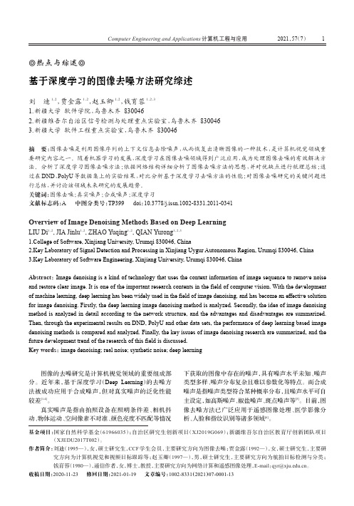
⦾热点与综述⦾基于深度学习的图像去噪方法研究综述刘迪1,2,贾金露1,2,赵玉卿1,2,钱育蓉1,2,31.新疆大学软件学院,乌鲁木齐8300462.新疆维吾尔自治区信号检测与处理重点实验室,乌鲁木齐8300463.新疆大学软件工程重点实验室,乌鲁木齐830046摘要:图像去噪是利用图像序列的上下文信息去除噪声,从而恢复出清晰图像的一种技术,是计算机视觉领域重要研究内容之一。
随着机器学习的发展,深度学习在图像去噪领域得到广泛应用,成为处理图像去噪的有效解决方法。
分析了深度学习图像去噪方法;依据网络结构详细分析了图像去噪方法的思想,并对优缺点进行梳理总结;通过在DND 、PolyU 等数据集上的实验结果,对比分析基于深度学习去噪方法的性能;对图像去噪研究的关键问题进行总结,并讨论该领域未来研究的发展趋势。
关键词:图像去噪;真实噪声;合成噪声;深度学习文献标志码:A中图分类号:TP399doi :10.3778/j.issn.1002-8331.2011-0341Overview of Image Denoising Methods Based on Deep LearningLIU Di 1,2,JIA Jinlu 1,2,ZHAO Yuqing 1,2,QIAN Yurong 1,2,31.College of Software,Xinjiang University,Urumqi 830046,China2.Key Laboratory of Signal Detection and Processing in Xinjiang Uygur Autonomous Region,Urumqi 830046,China3.Key Laboratory of Software Engineering,Xinjiang University,Urumqi 830046,ChinaAbstract :Image denoising is a kind of technology that uses the context information of image sequence to remove noise and restore clear image.It is one of the important research contents in the field of computer vision.With the development of machine learning,deep learning has been widely used in the field of image denoising,and has become an effective solution for image denoising.Firstly,the deep learning image denoising method is analyzed.Secondly,the idea of image denoising method is analyzed in detail according to the network structure,and the advantages and disadvantages are summarized.Then,through the experimental results on DND,PolyU and other data sets,the performance of deep learning based image denoising methods is compared and analyzed.Finally,the key issues of image denoising research are summarized,and the future development trend of the research of this field is discussed.Key words :image denoising;real noise;synthetic noise;deep learning基金项目:国家自然科学基金(61966035);自治区研究生创新项目(XJ2019G069);新疆维吾尔自治区教育厅创新团队项目(XJEDU2017T002)。
yangyang翻译

yangyang翻译基于⼩波阈值技术的图像去噪摘要:⼩波变换让我们在表述信号⽅⾯表现出⾼度的不⾜和弊端。
⼩波阈值是⼀种信号估值技术,它探索了基于⼩波变换的图像去噪的能⼒。
这篇⽂章的⽬的是研究多种阈值技术,例如SureShrink,V isuShrink和BayeShrink等等,同时找出最适合于图像去噪的阈值技术。
⼀:引⾔在许多应⽤中,图像去噪都被⽤来从含噪信号中得到原始的信号的最佳评估图像。
去噪信号应该⽐我们转换过的图像含有更少的噪声。
⼩波变换,由于其出⾊的定位性能, 已迅速成为⼀个不可或缺的信号和图像处理⼯具,他可以为各种应⽤程序进⾏信号和图像处理,其中包括压缩和去噪[1,2,3)。
⼩波消噪试图去除出现在信号的噪声,同时保留信号特征,⽽不管它的频率成分。
它涉及到三个步骤:⼀个是直线⼩波变换,它是⾮线性的阈值的⼀步,⼀个是线性逆⼩波变换。
⼩波阈值(⾸先由Donoho [1, 2, 3]中提出)是⼀种信号的评估⽅法和功能,它探索了基于⼩波变换的图像去噪的能⼒。
它通过去除噪声系数来进⾏图像去噪,着相对于⼀些阈值来说是微不⾜道的,同时结果是简洁的⽽且有效地,极⼤的依赖于阈值参数的选择,以及阈值确定的选择,这在很⼤程度上去除了噪声。
研究⼈员已经开发出各种技巧,选择去噪参数等⽬前没有“最好”的通⽤阈值的确定⽅法。
这个项⽬的⽬的是为了研究各种阈值技术,包括SureShrink[1],VisuShrink[3]和[5]BayesShrink并决定最好的处理图像噪声的阈值⽅法。
2.1引⾔在图1中的⼩波系数的的绘图显⽰⼩系数被噪声能量所左右, 同时有⼀个很⼤的系数绝对值携带更多的信号信息噪⾳。
利⽤0来代替噪声系数和⼩波逆变换可能会得到含有更少的噪声图像。
Fig.1在实践领域和⼩波领域的噪声信号,注意这些系数的不⾜。
2.2软硬阈值软硬阈值是按照如下形式定义的,硬阈值函数定义为:Fig2硬阈值函数软阈值函数定义为:Fig3软阈值函数硬阈值是⼀种“要么保持要么去除”的⼀种函数,这种函数更能直观的反映出来。
基于各向异性扩散滤波的图像去噪研究

基于各向异性扩散滤波的图像去噪研究莫绍强【摘要】采用各向异性扩散滤波方法,研究图像处理中的去噪问题,通过分析扩散函数和扩散常数对滤波效果的影响,利用图像压缩中判别压缩质量好坏的峰值信噪比作为迭代终止条件,在有效去除图像噪声的同时,能够保持图像的边缘信息不被过度滤除.%An anisotropic diffusion filtering method is used to research the denoising problem in image processing.By analyzing the influence of diffusion function and diffusion constant on the filtering effect,the peak signal to noise ratio in image compression is used as the iteration termination condition.This algorithm can keep the edge information of the image from being excessively filtered while effectively removing the noise.【期刊名称】《内蒙古师范大学学报(自然科学汉文版)》【年(卷),期】2017(046)001【总页数】4页(P19-22)【关键词】图像去噪;各向异性扩散;边缘信息;迭代准则;扩散函数【作者】莫绍强【作者单位】重庆电子工程职业学院,重庆 401331【正文语种】中文【中图分类】TP391.41图像滤波和去噪是图像处理中非常基础和重要的技术,常用的方法是采用一种滤波器,在滤除图像噪声的同时,尽可能地保留图像中的结构和纹理等信息不被破坏.传统方法中的高斯、中值等滤波,虽然能够去除噪声,但是图像的细节如边缘信息等也被同时滤除.双边滤波[1]虽然可以兼顾去噪和保留边缘的特性,但是计算极其耗时,制约了它的实用性.各向异性扩散滤波[2]是一种兼顾去噪和保留图像边缘的方法,它模拟热量传递原理,在同质区域热量可以扩散,而在非同质区域(存在边缘的位置)热传递减弱.但是该方法需要设置一个迭代次数的参数,判定何时终止扩散处理.如果迭代次数过少,噪声滤除不完全,迭代次数过多,容易导致图像本身的边缘细节信息丢失.因此,如何得到一个自动选择迭代终止的条件,对滤波效果非常重要.文献 [3] 利用梯度阈值,构建了一个随着时间变化逐渐递减的函数作为迭代终止准则,但为了得到自适应参数,每次迭代时需要保留边缘信息; 文献 [6-7] 利用原始图像和去噪图像之间的保真程度作为终止条件,但去噪不充分.本文通过分析各向异性扩散滤波中,扩散函数和扩散常数对滤波效果的影响,利用压缩图像中判别压缩质量好坏的峰值信噪比作为迭代终止条件,在有效去除图像噪声的同时,能够保持图像的边缘信息不被过度滤除,为图像滤波和去噪研究提供参考.Perona等[2]提出的各向异性扩散滤波,采用的是一种扩散处理的方式,即在同质平坦区域使噪声逐步平滑,当遇到非同质的边界区域时,则抑制平滑,其数学表达为(,t)=·(c(,t)I(,t))其中: I(,t)是待处理的图像; t表示迭代次数; c是一个关于图像梯度的单调递减扩散函数:c(,t)=f().(2)式可以根据图像的局部信息控制扩散强度,图像的边缘保留以及噪声滤除就是通过扩散函数来控制的.常用的两个扩散函数如下:c1(,t)(α>0),c2(,t)=exp ,其中K为扩散常数.从扩散函数的表达式可以看出,K值在很大程度上决定了同质区域和非同质区域的界线,对滤波效果的影响很大.令Φ表示扩散函数和梯度的乘积关系,有Φ(,t)=c(,t)I(,t).选择不同的扩散函数,Φ的处理效果也会不同.如图1所示,虚线和实线分别是取c1和c2为扩散函数时Φ的分布,可以看出,当K≫时,Φ值趋于0,可以将平坦区域平滑; 当K≪时,可以保留图像的边缘信息; 当噪声梯度约等于K时,可以噪声滤除.所以,根据图像噪声引起的梯度强弱选择合理的K值,就可以很好地将噪声去除.对于二维图像滤波,可以使用4邻域上的扩散滤波,分别代表在东南西北4个方向上扩散,滤波过程的表达式为(x,y,t)=≈ (,y,t)(I(x+Δx,y,t)-I(x,y,t))- c(,y,t)(I(x,y,t)-I(x-Δx,y,t))(x,,t)(I(x,y+Δy,t)-I(x,y,t))- c(x,,t)(I(x,y,t)-I(x,y-Δy,t))Δx=Δy=1.2.1 扩散函数和扩散常数扩散函数c是关于图像梯度的函数.图2是扩散常数K=0.05时,采用不同扩散函数的图像处理效果,其中第1排图像采用扩散函数c1,第2排图像采用扩散函数c2,迭代次数从左到右分别为2,8,64,128次.从对比效果可以看出,采用扩散函数c2对图像进行处理,得到的对比度大于扩散函数c1.从对比实验发现,K取较大值时,只有大的轮廓边缘保留下来,更多的细节边缘被滤除,这是因为梯度较小的区域被认为是噪声部分,只有梯度远远大于K的轮廓被部分保留下来.因此,参数K的选择,决定了哪些区域属于同质区域,哪些属于非同质区域. 图3是扩散函数和扩散常数对滤波结果的影响,可以看出,K值相同时,以c1作为扩散函数保留下来的边缘梯度弱于c2扩散函数,但是同质区域更平滑,这可以作为处理不同图像时,预计达到某种效果的参考依据.2.2 迭代终止条件从图2和图3可以看出,随着迭代次数的不断增多,图像细节信息会逐渐减少,因此只有设置一个终止迭代的条件,才能得到最佳滤波效果.本文利用图像压缩中判断压缩质量好坏的峰值信噪比PSNR[6]作为迭代终止条件,PSNR=10 log10(MAXI)-10 log10(MSE),其中: 2,称为均方误差(mean squared error); MAX是图像的灰度级,一般取值255; I是上一次迭代的图像,K是当前迭代处理后的图像.由于多次迭代后噪声已被去除,所以PSNR的变化率会很小.图4是各向异性扩散的去噪迭代过程,图中从左至右分别为原始噪声图和迭代56,148,280次后的效果.其中噪声图像是在原始图像上加了均值为0、标准偏差为0.02的高斯噪声.本文取迭代前后差异小于阈值T时为迭代终止条件,通常取T=0.01.图4中,迭代终止在第148次,这时图像噪声被滤除,且细节保持较好,而迭代56次时噪声保留太多,迭代280次时图像的边缘被过度滤除.因此本文设置的迭代终止条件得到了比较理想的结果.基于各向异性扩散滤波的图像处理方法,不仅可以去除噪声,而且能更好地保护边缘信息不被滤除,较之传统的高斯、中值等滤波方法有很大的优势,在图像增强方面有很好的应用前景.本文提出的迭代终止条件简单易实现,为滤除噪声和避免边缘被过度滤除提供了一种平衡方法.另外,影响图像滤波效果的因素除了迭代次数外,还有扩散参数K,该参数往往与图像噪声梯度相关,如何估算图像的噪声梯度信息,合理设置参数K的大小,是需要进一步研究的内容.【相关文献】[1] TOMASI C,MANDUCHI R. Bilateral filtering for gray and color images [C]//ICCV,1998:839-846.[2] PERONA P,MALIK J. Scale-space and edge detection using anisotropic diffusion [J]. IEEE TPAMI,1990,12(7):629-639.[3] X Li,T Chen. Nonlinear diffusion with multiple edginess thresholds [J]. Pattern Recognition,1994,27(8):1029-1037.[4] Gilboa G,Sochen N,Zeevi Y Y. Forward-and-backward diffusion processes for adaptive image enhancement and denoising [J]. IEEE Transactions on ImageProcessing,2002,11(7):689-703.[5] Weickert J. Applications of nonlinear diffusion in image processing and computer vision [J]. Acta Mathematica Universitatis Comenianae,2001,70:33-50.[6] Huynh-Thu Q,Ghanbari M. Scope of validity of PSNR in image/video quality assessment [J]. Electronics Letters,2008,44(13):800-801.。
一种基于小波的眼伪影校正的脑电图去噪技术毕业论文外文翻译

一种基于小波的眼伪影校正的脑电图去噪技术毕业论文外文翻译A WA VELET BASED DE-NOISING TECHNIQUE FOROCULAR ARTIFACT CORRECTION OF THEELECTROENCEPHALOGRAMTatjana Zikov, Stéphane Bibian, Guy A. Dumont, Mihai Huzmezan Department of Electrical and Computer Engineering, the University of BritishColumbia, BC, CANADA.Abstract –This paper investigates a wavelet based denoising of the electroencephalogram (EEG) signal to correct for the presence of the ocular artifact (OA).The proposed technique is based on an over-complete wavelet expansion of the EEG as follows: i) a stationary wavelet transform (SWT) is applied to the corrupted EEG; ii) the thresholding of the coefficients in the lower frequency bandsis performed; iii) the de-noised signal is reconstructed. This paper demonstrates the potential of the proposed technique for successful OA correction. The advantage over conventional methods is that there is no need for the recording of the electrooculogram (EOG) signal itself. The approach works both for eye blinks and eye movements. Hence, there is no need to discriminate between different artifacts. To allow for a proper comparison, the contaminated EEG signals as well as the corrected signals are presented together with their corresponding power spectra.Keywords-stationary wavelet transform (SWT), electroencephalogram (EEG), electrooculogram (EOG), ocular artifact (OA).I. INTRODUCTIONThe electroencephalogram (EEG) gives researchers a non-invasive insight into the intricacy of the human brain. It is a valuable tool for clinicians in numerous applications, from the diagnosis of neurological disorders, to the clinical monitoring of depth of anesthesia. For awake healthy subject, normal EEG amplitude is in the order of 20-50μV.The EEG is very susceptible to various artifacts, causing problems for analysis and interpretation. In current data acquisition, eye movement and blink related artifacts are often dominant over other electrophysiological contaminating signals (e.g. heart and muscle activity, head and body movements), as well as external interferences due to power sources. Eye movements and blinks produce a large electrical signal around the eyes (in the order of mV), known as electrooculogram (EOG), which spreads across the scalp and contaminates the EEG. These contaminating potentials arecommonly referred to as ocular artifact (OA).The rejection of epochs contaminated with OA usually leads to a substantial loss of data. Asking subjects not to blink or move their eyes or to keep their eyes shut and still, is often unrealistic or inadequate. The fact that the subject is concentrating on fulfilling these requirements might itself influence his EEG. Hence, devising a method for successful removal of ocular artifacts (OA) from EEG recordings has been and still is a major challenge.Widely used time-domain regression methods involve the subtraction of some portion of the recorded EOG from the EEG [1, 2]. They assume that the propagation of ocular potentials is volume conducted, frequency independent and without any time delay. However, Gasser et al. in [3] argued that the scalp is not a perfect volume conductor, and thus, attenuates some frequencies more than others. Consequently, frequency domain regression was proposed. In addition, no significant time delay was found, which was in consistency with the EOG being volume conducted.In [4]it was reported that, in reality, the frequency dependence does not seem to be very pronounced, while the assumption of no measurable delay was confirmed. Thus, while some researchers support the frequency domain approach for EOG correction [3, 5], others disputed its advantages [4, 6, 7]. However, neither time nor frequency regression techniques take into account the propagation of the brain signals into the recorded EOG. Thus a portion of relevant EEG signal is always cancelled out along with the artifact. Further, these techniques mainly use different correction coefficients for eye blinks versus eye movements. They also heavily depend on the regressing EOG channel.In addition, Croft and Barry [7]demonstrated that the propagation of the EOG across the scalp is constant with respect to ocular artifact types and frequencies. They proposed a more sophisticated regression method (the aligned-artifact average solution) that corrects blinks and eye movement artifacts together, and made possible the adequate correction for posterior sites [6]. They claim that the influence of the EEG-to-EOG propagation has been minimized in their method.In an attempt to overcome the problem of the EEG-to-EOG propagation, a multiple source eye correction method has been proposed by Berg and Scherg [8]. In this method, the OA was estimated based on the source eye activity ratherthan the EOG signal. The method involves obtaining an accurate estimate of the spatial distribution of the eye activity from calibration data, which is a rather difficult task.Due to its decorrelation efficiency, the principal component analysis (PCA) has been applied for OA removal from the multi-channel EEG and it outperformed the previously mentioned methods. However, it has been shown that PCA cannot fully separate OA from the EEG when comparable amplitudes are encountered [9].Recently, independent component analysis (ICA) has demonstrated a superior potential for the removal of a wide variety of artifacts from the EEG[10, 11], even in a case of comparable amplitudes. ICA simultaneously and linearly unmixed multi-channel scalp recordings into independent components, that are often physiologically plausible. Also, there is no need for a reference channel corresponding to each artifact source. However, ICA artifact removal is not yet fully automated and requires visual inspection of the independent components in order to decide their removal.Other attempts have been based on different adaptive signal processing techniques [12-16]. The performance of these methods also relies on a cerebral activity to minimally contaminate the EOG reference.The EEG may contain pathological signals, which resemble OA. Thus, these signals are most likely to be removed from the EEG recordings, leading to erroneous diagnosis. Therefore, it is important to distinguish between artifacts and pathological EEG signals prior to artifact removal. Artificial intelligence techniques prove to be somehow helpful in achieving this goal [17].Our aim is to present a real-time OA removal technique, based on stationary wavelet transform (SWT) de-noising of a single frontal channel EEG. The proposed technique is based on an over-complete wavelet expansion of the EEG as follows: i) a stationary wavelet transform is applied to the corrupted EEG; ii) the thresholding of the coefficients in the lower frequency bands is performed; iii) the de-noised signal is reconstructed. No reference EOG channel is needed and the same approach is used for both the blinks and eye movement artifacts.The time and frequency characteristics of OA are addressed in Section II, while Section III discusses the proposed method. Results are further presented in Section IV.II. OCULAR ARTIFACTSThere are two different originating phenomena for ocular potentials [1, 18, 19]. There is a potential difference of about 100 mV between a positively charged cornea and negative retina of the human eye, thus forming an electrical dipole (i.e. corneo-retinal dipole). Firstly, the rotation of the eyeball results in changes of the electrical field across the skull. Secondly, eye blinks are usually not associated with ocular rotation; however, the eyelids pick up the positive potential as they slide over the cornea. T his creates an electrical field that is also propagated through the skull. Hence, ocular potentials spread across the scalp and superimpose on the EEG.The mechanism of origin (eye movements versus eye blinks) and the direction of eye movements determine the resulting EOG wave shape. Vertical, horizontal and round eye movements usually result in square-shaped EOG waveforms, while blinks are spike-like waves.Fig.1 Uncontaminated Baseline EEG andVarious Artifacts(a) Uncontaminated baseline EEG (b) EEGcontaminated with slow blink artifact (c) EEG contaminated with fast blink artifact (d) EEG contaminated with vertical eye movement artifact (e) EEG contaminated with horizontal eye movement artifact (f) EEG contaminated with round eye movement artifactOcular artifacts decrease rapidly with the distance from the eyes [18]. Therefore, the most severe interference occurs in the EEG recorded by the electrodes placed on the patient's forehead. Yet, this is the most convenient region for their placement. Thereto, the frontal and prefrontal lobes, which are at the origin of higher cognitive functions, are located directly behind the forehead. Therefore, the task of EOG correction for frontal channels is challenging.For the purpose of this paper, we have acquired EEG data from an awake healthy male subject. A single frontal channel was recorded, corresponding to the Fpz electrode placement in the nomenclature of the International 10-20 System. The baseline EEG and five various artifacts were recorded in the following fashion. For each artifact, the subject was first instructed to keep his eyes shut and still. Sixty seconds of presumably uncontaminated baseline EEG was thus recorded. Then, for the next 60 seconds, the subject was instructed to blink or move his eyes in a predetermined fashion. Finally, another resting period of 60 seconds with no EOG activity was recorded. Five ocular artifacts were recorded in this fashion: slow blinks (1 blink per 2 seconds), fast blinks (2 blinks per second), vertical, horizontal and round eye movements. The signal was notch filtered at 50-60 Hz and sampled at 128 Hz.Fig.2 Power Spectra of UncontaminatedBaseline EEG and Various Artifacts (a)Uncontaminated baseline EEG and other resting periods (b) EEG contaminated with slow blink artifact (c) EEG contaminated with fast blink artifact (d) EEG contaminated with vertical eye movement artifact (e) EEG contaminated with horizontal eye movement artifact (f) EEG contaminated with round eye movement artifactFig. 2 clearly shows that OA are large, transient slow waves. They occupy the lower frequency range; from 0 Hz up to 6-7 Hz for the eye movement artifacts, and typically up to the alpha band (8-13 Hz), excluding very low frequencies, for the eye blinks. This is a well-known and documented result [3], which our experiments proved consistent with. Clearly, OA amplitudes are of a much higher order than those of the uncontaminated EEG and have a characteristic pattern of changes. Vertical eye movement artifacts (Fig. 2.d) also seem to produce a rise in the higher frequencies. However, this is most likely due to the increased muscle activity, and it is also present to a lesser degree for the other two eye movements (horizontal - Fig. 2.e, and round - Fig. 2.f).III. WA VELET-BASED DE-NOISINGA.Problem StatementAs previously mentioned, the EOG is the non-cortical activity that contaminates the EEG recordings. Thus, since the brain and eye activities have physiologically separate sources, we will assume the recorded EEG is a superposition of the true EEG and some portion of the EOG signal. Thus, we have:offest true rec dc t EOG k t EEG t EEG +⋅+=)()()( (1)Where rec EEG is the recorded contaminated EEG , true EEG is due to thecortical activity, and EOG k ⋅is the propagated ocular artifact at the recording site. The dcoffset takes into account the zero mean value of the cortical EEG , since this might not be true for the recorded EEG due to the process of data acquisition.We are interested in estimating the ocular artifact based on the analysis of the recorded EEG . By subtracting it from the contaminated EEG , we will then obtain a corrected EEG , which minimizes the effect of the ocular artifact and gives an appropriate representation of the true cortical EEG .The true EEG is a noise-like signal. We can not observe any clear patterns within it, nor can we simply correlate the particular underlying events with its wave shape [20].Furthermore, in the awake, conscious state, neurons are firing in a more independent fashion. As a result of this resynchronizations, the awake EEG signal is even more random-appearing. The EOG removal can be approached by recovering the regression function (EOG k ⋅ ) from the recorded data. For this purpose, in the last decade, wavelet thresholding has emerged as a simple, yet effective technique for de-noising [21].B. Wavelet ThresholdingThe main statistical application of wavelet thresholding is a nonparametric estimation of the regression function f , based on observations i s at time points i t . The i s observations are modeled as:)2(,2,1,)(n i i i N N i t f s ==+= ε (2)Where i εare independent and identically distributed ),0(2σN random variables at equally spaced time points i t .Due to the orthogonality of the wavelet transform, we are allowed to perform filtering in the space of wavelet coefficients. The procedure for suppressing the noise involves: i) finding the coefficients of the wavelet transform of {si}; ii) comparing each wavelet coefficient against an appropriate threshold;iii) keeping only those coefficients larger than a threshold; and iv) applying an inverse wavelet transform to obtain an estimate of f. The assumption is that large coefficients kept after thresholding belong to the function to be estimated, and those discarded belong to the noise. This is a fair assumption due to the good energy compaction of the wavelet transform. Some of the function coefficients might eventually be discarded since they are of the same level as the noise coefficients. Thus, this denoising technique works well for functions whose wavelet transform results in only a few nonzero wavelet coefficients, like e.g. functions that are smooth almost everywhere, except for only a few abrupt changes [22].Special care has to be taken when choosing an appropriate threshold, which always involves the estimation of the noise variance 2σbased on the data.一种基于小波的眼伪影校正的脑电图去噪技术一、导言脑电图(EEG)使研究人员对复杂的人类大脑进行非侵入性的深入了解。