机器人工具箱仿真程序-Matlab
利用matlab的机器人试验仿真

选择MATLAB2016a版,高版本不能安装。
安装好按照下面的操作做出来,然后截图做成Word文档发给我。
MATLAB2016a版同学们网上下载安装,安装方法网上随便可找到。
机器人工具箱我发给你们。
一、将文件夹放到MATLAB安装文件夹指定目录下放到安装目录的toolbox文件夹下,如下图是笔者的电脑的位置,其中那个installation address是我自己取得名字,英语不好,不要见怪。
三、打开MATLAB软件,进行手动启动(1)打开matlab,依次点击file(文件)-setpath(设置路径)-add with subfolder (添加子文件夹),然后选择这个rvctools文件夹就好了,然后save(保存)-close (关闭)(2)在命令行窗口输入startup_rvc,回车,如图,显示了一段英语,我恩可以看到,版本是9.10。
本文主要是给大家一个系统的概念,如何用Matlab实现六轴机器人的建模和实现轨迹规划。
以后将会给大家讲解如何手写正逆解以及轨迹插补的程序。
程序是基于Matlab2016a,工具箱版本为Robotic Toolbox 9.10。
1.D-H建模三个两两相互垂直的XYZ轴构成欧几里得空间,存在六个自由度:沿XYZ 平移的三个自由度,绕XYZ旋转的三个自由度。
在欧几里得空间中任意线性变换都可以通过这六个自由度完成。
Denavit-Hartenberg提出的D-H参数模型能满足机器人学中的最小线性表示约定,用4个参数就能描述坐标变换:绕X轴平移距离a;绕X轴旋转角度alpha;绕Z轴平移距离d;绕Z轴旋转角度theta。
2.标准D-H模型和改进D-H模型对比来看参数并没有改变,标准的D-H 模型是将连杆的坐标系固定在该连杆的输出端(下一关节),也即坐标系i-1与关节i对齐;改进的D-H模型则是将坐标系固定在该连杆的输入端(上一关节),也即坐标系i-1与关节对齐i-1。
matlab中robotics toolbox的应用
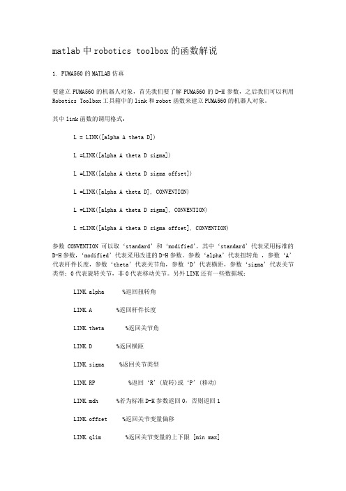
matlab中robotics toolbox的函数解说1. PUMA560的MATLAB仿真要建立PUMA560的机器人对象,首先我们要了解PUMA560的D-H参数,之后我们可以利用Robotics Toolbox工具箱中的link和robot函数来建立PUMA560的机器人对象。
其中link函数的调用格式:L = LINK([alpha A theta D])L =LINK([alpha A theta D sigma])L =LINK([alpha A theta D sigma offset])L =LINK([alpha A theta D], CONVENTION)L =LINK([alpha A theta D sigma], CONVENTION)L =LINK([alpha A theta D sigma offset], CONVENTION)参数CONVENTION可以取‘standard’和‘modified’,其中‘standard’代表采用标准的D-H参数,‘modified’代表采用改进的D-H参数。
参数‘alpha’代表扭转角,参数‘A’代表杆件长度,参数‘theta’代表关节角,参数‘D’代表横距,参数‘sigma’代表关节类型:0代表旋转关节,非0代表移动关节。
另外LINK还有一些数据域:LINK.alpha %返回扭转角LINK.A %返回杆件长度LINK.theta %返回关节角LINK.D %返回横距LINK.sigma %返回关节类型LINK.RP %返回‘R’(旋转)或‘P’(移动)LINK.mdh %若为标准D-H参数返回0,否则返回1LINK.offset %返回关节变量偏移LINK.qlim %返回关节变量的上下限 [min max]LINK.islimit(q) %如果关节变量超限,返回 -1, 0, +1LINK.I %返回一个3×3 对称惯性矩阵LINK.m %返回关节质量LINK.r %返回3×1的关节齿轮向量LINK.G %返回齿轮的传动比LINK.Jm %返回电机惯性LINK.B %返回粘性摩擦LINK.Tc %返回库仑摩擦LINK.dh return legacy DH rowLINK.dyn return legacy DYN row其中robot函数的调用格式:ROBOT %创建一个空的机器人对象ROBOT(robot) %创建robot的一个副本ROBOT(robot, LINK) %用LINK来创建新机器人对象来代替robotROBOT(LINK, ...) %用LINK来创建一个机器人对象ROBOT(DH, ...) %用D-H矩阵来创建一个机器人对象ROBOT(DYN, ...) %用DYN矩阵来创建一个机器人对象2.变换矩阵利用MATLAB中Robotics Toolbox工具箱中的transl、rotx、roty和rotz可以实现用齐次变换矩阵表示平移变换和旋转变换。
在MATLAB中进行机器人编程和仿真
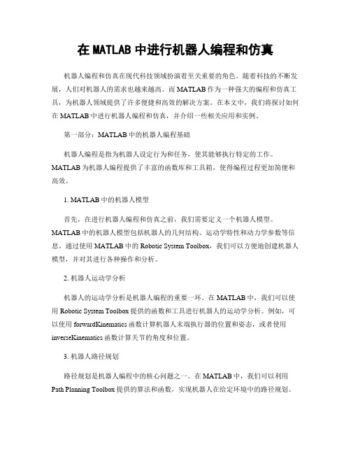
在MATLAB中进行机器人编程和仿真机器人编程和仿真在现代科技领域扮演着至关重要的角色。
随着科技的不断发展,人们对机器人的需求也越来越高。
而MATLAB作为一种强大的编程和仿真工具,为机器人领域提供了许多便捷和高效的解决方案。
在本文中,我们将探讨如何在MATLAB中进行机器人编程和仿真,并介绍一些相关应用和实例。
第一部分:MATLAB中的机器人编程基础机器人编程是指为机器人设定行为和任务,使其能够执行特定的工作。
MATLAB为机器人编程提供了丰富的函数库和工具箱,使得编程过程更加简便和高效。
1. MATLAB中的机器人模型首先,在进行机器人编程和仿真之前,我们需要定义一个机器人模型。
MATLAB中的机器人模型包括机器人的几何结构、运动学特性和动力学参数等信息。
通过使用MATLAB中的Robotic System Toolbox,我们可以方便地创建机器人模型,并对其进行各种操作和分析。
2. 机器人运动学分析机器人的运动学分析是机器人编程的重要一环。
在MATLAB中,我们可以使用Robotic System Toolbox提供的函数和工具进行机器人的运动学分析。
例如,可以使用forwardKinematics函数计算机器人末端执行器的位置和姿态,或者使用inverseKinematics函数计算关节的角度和位置。
3. 机器人路径规划路径规划是机器人编程中的核心问题之一。
在MATLAB中,我们可以利用Path Planning Toolbox提供的算法和函数,实现机器人在给定环境中的路径规划。
通过设置起始点和目标点,以及环境的障碍物信息,可以使用MATLAB中的路径规划算法自动生成机器人的轨迹,使其能够高效地避开障碍物并到达目标位置。
第二部分:机器人编程和仿真的应用案例机器人编程和仿真在许多领域都有广泛的应用。
下面将介绍两个典型的应用案例,以展示MATLAB在机器人领域的强大功能。
1. 机器人控制系统设计机器人控制系统是机器人编程中的关键环节。
MATLAB机器人仿真程序
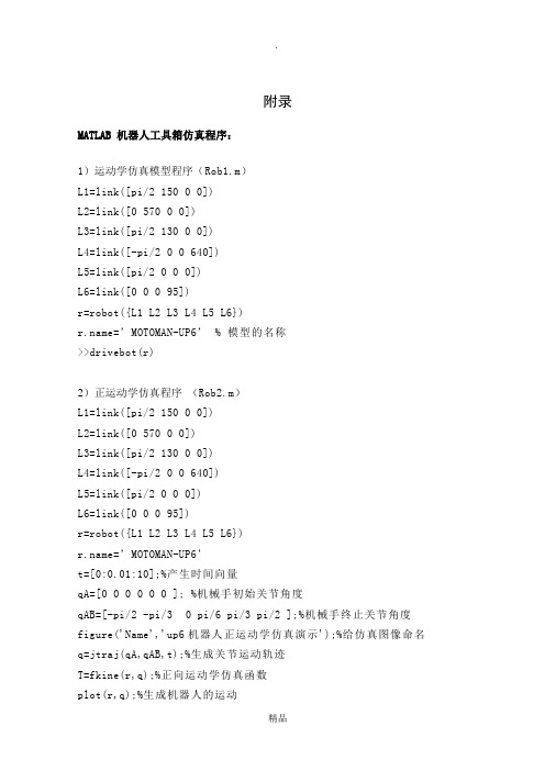
附录MATLAB 机器人工具箱仿真程序:1)运动学仿真模型程序(Rob1.m)L1=link([pi/2 150 0 0])L2=link([0 570 0 0])L3=link([pi/2 130 0 0])L4=link([-pi/2 0 0 640])L5=link([pi/2 0 0 0])L6=link([0 0 0 95])r=robot({L1 L2 L3 L4 L5 L6})=’MOTOMAN-UP6’ % 模型的名称>>drivebot(r)2)正运动学仿真程序(Rob2.m)L1=link([pi/2 150 0 0])L2=link([0 570 0 0])L3=link([pi/2 130 0 0])L4=link([-pi/2 0 0 640])L5=link([pi/2 0 0 0])L6=link([0 0 0 95])r=robot({L1 L2 L3 L4 L5 L6})=’MOTOMAN-UP6’t=[0:0.01:10];%产生时间向量qA=[0 0 0 0 0 0 ]; %机械手初始关节角度qAB=[-pi/2 -pi/3 0 pi/6 pi/3 pi/2 ];%机械手终止关节角度figure('Name','up6机器人正运动学仿真演示');%给仿真图像命名q=jtraj(qA,qAB,t);%生成关节运动轨迹T=fkine(r,q);%正向运动学仿真函数plot(r,q);%生成机器人的运动figure('Name','up6机器人末端位移图')subplot(3,1,1);plot(t, squeeze(T(1,4,:)));xlabel('Time (s)');ylabel('X (m)');subplot(3,1,2);plot(t, squeeze(T(2,4,:)));xlabel('Time (s)');ylabel('Y (m)');subplot(3,1,3);plot(t, squeeze(T(3,4,:)));xlabel('Time (s)');ylabel('Z (m)');x=squeeze(T(1,4,:));y=squeeze(T(2,4,:));z=squeeze(T(3,4,:));figure('Name','up6机器人末端轨迹图'); plot3(x,y,z);3)机器人各关节转动角度仿真程序:(Rob3.m)L1=link([pi/2 150 0 0 ])L2=link([0 570 0 0])L3=link([pi/2 130 0 0])L4=link([-pi/2 0 0 640])L5=link([pi/2 0 0 0 ])L6=link([0 0 0 95])r=robot({L1 L2 L3 L4 L5 L6})='motoman-up6't=[0:0.01:10];qA=[0 0 0 0 0 0 ];qAB=[ pi/6 pi/6 pi/6 pi/6 pi/6 pi/6]; q=jtraj(qA,qAB,t);Plot(r,q);subplot(6,1,1);plot(t,q(:,1));title('转动关节1');xlabel('时间/s');ylabel('角度/rad');subplot(6,1,2);plot(t,q(:,2));title('转动关节2');xlabel('时间/s');ylabel('角度/rad');subplot(6,1,3);plot(t,q(:,3));title('转动关节3');xlabel('时间/s');ylabel('角度/rad');subplot(6,1,4);plot(t,q(:,4));title('转动关节4');xlabel('时间/s');ylabel('角度/rad' );subplot(6,1,5);plot(t,q(:,5));title('转动关节5');xlabel('时间/s');ylabel('角度/rad');subplot(6,1,6);plot(t,q(:,6));title('转动关节6');xlabel('时间/s');ylabel('角度/rad');4)机器人各关节转动角速度仿真程序:(Rob4.m)t=[0:0.01:10];qA=[0 0 0 0 0 0 ];%机械手初始关节量qAB=[ 1.5709 -0.8902 -0.0481 -0.5178 1.0645 -1.0201]; [q,qd,qdd]=jtraj(qA,qAB,t);Plot(r,q);subplot(6,1,1);plot(t,qd(:,1));title('转动关节1');xlabel('时间/s');ylabel('rad/s');subplot(6,1,2);plot(t,qd(:,2));title('转动关节2');xlabel('时间/s');ylabel('rad/s');subplot(6,1,3);plot(t,qd(:,3));title('转动关节3');xlabel('时间/s');ylabel('rad/s');subplot(6,1,4);plot(t,qd(:,4));title('转动关节4');xlabel('时间/s');ylabel('rad/s' );subplot(6,1,5);plot(t,qd(:,5));title('转动关节5');xlabel('时间/s');ylabel('rad/s');subplot(6,1,6);plot(t,qd(:,6));title('转动关节6');xlabel('时间/s');ylabel('rad/s');5)机器人各关节转动角加速度仿真程序:(Rob5.m)t=[0:0.01:10];%产生时间向量qA=[0 0 0 0 0 0]qAB =[1.5709 -0.8902 -0.0481 -0.5178 1.0645 -1.0201]; [q,qd,qdd]=jtraj(qA,qAB,t);figure('name','up6机器人机械手各关节加速度曲线');subplot(6,1,1);plot(t,qdd(:,1));title('关节1');xlabel('时间 (s)');ylabel('加速度 (rad/s^2)');subplot(6,1,2);plot(t,qdd(:,2));title('关节2');xlabel('时间 (s)');ylabel('加速度 (rad/s^2)');subplot(6,1,3);plot(t,qdd(:,3));title('关节3');xlabel('时间 (s)');ylabel('加速度 (rad/s^2)')subplot(6,1,4);plot(t,qdd(:,4));title('关节4');xlabel('时间 (s)');ylabel('加速度 (rad/s^2)')subplot(6,1,5);plot(t,qdd(:,5));title('关节5');xlabel('时间 (s)');ylabel('加速度 (rad/s^2)')subplot(6,1,6);plot(t,qdd(:,6));title('关节6');xlabel('时间 (s)');ylabel('加速度 (rad/s^2)')如有侵权请联系告知删除,感谢你们的配合!。
基于MATLAB的六自由度工业机器人运动分析和仿真
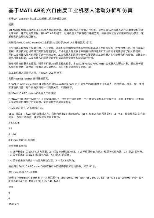
基于MATLAB的六⾃由度⼯业机器⼈运动分析和仿真基于MATLAB 的六⾃由度⼯业机器⼈运动分析及仿真摘要:以FANUC ARC mate100⼯业机器⼈为研究对象,对其机构和连杆参数进⾏分析,采⽤D-H 法对机器⼈进⾏正运动学和逆运动学分析,建⽴运动学⽅程。
在MATLAB 环境下,运⽤机器⼈⼯具箱进⾏建模仿真,仿真结果证明了所建⽴的运动学正、逆解模型的合理性和正确性。
关键词:FANUC ARC mate100⼯业机器⼈; 运动学; MATLAB 建模仿真 1引⾔⼯业机器⼈技术是在控制⼯程、⼈⼯智能、计算机科学和机构学等多种学科的基础上发展起来的⼀种综合性技术。
经过多年的发展,该项技术已经取得了实质性的进步[1]。
⼯业机器⼈的发展⽔平随着科技的进步和⼯业⾃动化的需求有了很⼤的提⾼,同时⼯业机器⼈技术也得到了进⼀步的完善。
⼯业机器⼈的运动学分析主要是通过⼯业机器⼈各个连杆和机构参数,以确定末端执⾏器的位姿。
⼯业机器⼈的运动学分析包括正运动学分析和逆运动学分析。
随着对焊接件要求的提⾼,弧焊等机器⼈的需求越来越多。
本⽂就以FANUC ARC mate100机器⼈为研究对象,通过分析机构和连杆参数,运⽤D-H 参数法建⽴坐标系,求出连杆之间的位姿矩阵,建⽴⼯业机器⼈运动学⽅程。
并在MATLAB 环境下,利⽤RoboticsToolbox 进⾏建模仿真。
2 FANUC ARC mate100 D-H 坐标系的建⽴mate100是FANUC 公司⽣产的6⾃由度⼯业机器⼈,包括底座、机⾝、臂、⼿腕和末端执⾏器,每个⾃由度对应⼀个旋转关节,如图1所⽰。
图1FANUC ARC mate 100机器⼈三维模型DENAVIT 和HARTENBERG 于1955年提出了⼀种为关节链中的每⼀个杆件建⽴坐标系的矩阵⽅法,即D-H 参数法,在机器⼈运动学分析得到了⼴泛运⽤。
采⽤这种⽅法建⽴坐标系:(1) Z i 轴沿关节i +1的轴线⽅向。
基于MATLABRoboticsToolbox的机器人学仿真实验教学-精品文档
基于MATLAB Robotics Toolbox 的机器人学仿真实验教学机器人学是一门高度交叉的前沿学科方向, 也是自动化和机电工程等相关专业的一门重要专业基础课。
在机器人学的教学和培训中, 实验内容一直是授课的重点和难点。
实物机器人通常是比较昂贵的设备, 这就决定了在实验教学中不可能运用许多实际的机器人来作为教学和培训的试验设备。
由于操作不方便、体积庞大等原因, 往往也限制了实物机器人在课堂授课时的应用。
此外, 由于计算量、空间结构等问题,当前大多数机器人教材只能以简单的两连杆机械手为例进行讲解,而对于更加实际的 6 连杆机械手通常无法讲解得很清楚。
因此, 各式各样的机器人仿真系统应运而生。
经过反复的比较,我们选择了MATLAB RoboticsToolbox [1] 来进行机器人学的仿真实验教学。
MATLABRobotics Toolbox 是由澳大利亚科学家Peter Corke开发和维护的一套基于MATLAB勺机器人学工具箱,当前最新版本为第8版,可在该工具箱的主页上免费下载提供了机器人学研究(petercorke/robot/) 。
Robotics Toolbox中的许多重要功能函数, 包括机器人运动学、动力学、轨迹规划等。
该工具箱可以对机器人进行图形仿真, 并能分析真实机器人控制时的实验数据结果, 因此非常适宜于机器人学的教学和研究。
本文简要介绍了Robotics Toolbox 在机器人学仿真实验教学中的一些应用, 具体内容包括齐次坐标变换、机器人对象构建、机器人运动学求解以及轨迹规划等。
1坐标变换机器人学中关于运动学和动力学最常用的描述方法是矩阵法, 这种数学描述是以四阶方阵变换三维空间点的齐次坐标为基础的[2] 。
如已知直角坐标系{A} 中的某点坐标,那么该点在另一直角坐标系{B} 中的坐标可通过齐次坐标变换求得。
一般而言齐次变换矩阵是4X4的方阵,具有如下形式: 和分别表示{A}{B} 两坐标系之间的旋转变换和平移变换。
MATLAB机器人仿真程序
MATLAB仿真程序1、摘要:简要介绍仿真程序的目的和应用领域。
2、简介2.1 背景:介绍仿真技术的背景和发展趋势。
2.2 目标:阐述本文档旨在实现的目标和预期成果。
2.3 使用范围:说明本文档适用的MATLAB版本和相关工具。
3、系统需求3.1 软件需求:列出在运行仿真程序时需要的MATLAB版本和相关工具。
3.2 硬件需求:描述在运行仿真程序时所需的最低硬件配置要求。
4、数据准备4.1 输入数据:说明仿真程序所需的输入数据,包括模型、环境参数、运动规划等。
4.2 数据处理:描述对输入数据进行预处理和转换的方法和算法。
5、仿真实现5.1 建模:介绍如何使用MATLAB建立模型。
5.2 运动规划:讲解如何使用运动规划算法的轨迹。
5.3 运动控制:详细说明如何控制的关节运动和末端执行器的运动。
6、结果分析6.1 数据保存:指示如何保存仿真过程和结果的数据。
6.2 数据可视化:说明如何使用MATLAB绘制仿真结果图表。
6.3 结果评估:解析实验结果,验证仿真程序的准确性和可行性。
7、总结和下一步工作简要总结此次仿真程序的实现和结果,提出改进的建议,并探讨下一步工作的方向。
附件:本文档涉及的附件包括:- 模型文件- 仿真环境场景文件- 运动规划算法实现代码- 仿真结果数据文件法律名词及注释:1、版权:著作权法规定的著作物享有的法律保护。
2、许可证:根据许可证要求,特定行为(如使用、复制、修改)被允许或拒绝使用。
3、商标:商标是注册商标办公室注册的标志,用于识别产品或服务来源。
4、法律依据:涉及到法律的相关内容,应根据当地法律依据进行操作。
matlab机器人运动学仿真代码

matlab机器人运动学仿真代码以下是一个简单的MATLAB机器人运动学仿真代码示例,假设机器人是一个二维平面上的两轴机器人,其中关节1和关节2的长度分别为L1和L2:matlab.% 定义关节长度。
L1 = 1;L2 = 1;% 定义关节角度。
theta1 = 0:0.01:2pi; % 关节1角度范围。
theta2 = 0:0.01:2pi; % 关节2角度范围。
% 初始化末端点坐标。
x = zeros(length(theta1), length(theta2));y = zeros(length(theta1), length(theta2));% 计算末端点坐标。
for i = 1:length(theta1)。
for j = 1:length(theta2)。
x(i,j) = L1 cos(theta1(i)) + L2 cos(theta1(i) + theta2(j));y(i,j) = L1 sin(theta1(i)) + L2 sin(theta1(i) + theta2(j));end.end.% 绘制机器人末端点轨迹。
figure;plot(x(:), y(:), 'b.');xlabel('X');ylabel('Y');title('机器人末端点轨迹');这段代码实现了一个简单的两轴机器人的运动学仿真。
首先定义了机器人的关节长度和关节角度范围,然后计算了末端点的坐标,并绘制了机器人末端点的轨迹。
当然,实际的机器人运动学仿真会更加复杂,涉及到不同类型的机器人和运动学模型,但这段代码可以作为一个简单的起点,帮助你开始进行机器人运动学仿真的工作。
MATLAB机器人仿真程序
MATLAB机器人仿真程序哎呀,说起 MATLAB 机器人仿真程序,这可真是个有趣又充满挑战的领域!我还记得有一次,我带着一群学生尝试做一个简单的机器人行走仿真。
那时候,大家都兴奋极了,眼睛里闪着好奇的光。
我们先从最基础的开始,了解 MATLAB 这个工具的各种函数和命令。
就像是给机器人准备好各种“零部件”,让它能顺利动起来。
比如说,我们要设定机器人的初始位置和姿态,这就好像是告诉机器人“嘿,你从这里出发,站好啦!”然后,再通过编程来控制它的运动轨迹。
有的同学想让机器人走直线,有的同学想让它拐个弯,还有的同学想让它走个复杂的曲线。
在这个过程中,可遇到了不少问题呢。
有个同学不小心把坐标设置错了,结果机器人“嗖”地一下跑到了不知道哪里去,大家哄堂大笑。
还有个同学在计算速度和加速度的时候出了差错,机器人的动作变得奇奇怪怪的,像是在跳“抽筋舞”。
不过,大家并没有气馁,而是一起努力找错误,修改代码。
终于,当我们看到那个小小的机器人按照我们设想的轨迹稳稳地行走时,那种成就感简直无法形容。
回到 MATLAB 机器人仿真程序本身,它其实就像是一个神奇的魔法盒子。
通过输入不同的指令和参数,我们可以创造出各种各样的机器人运动场景。
比如说,我们可以模拟机器人在不同地形上的行走,像是平坦的地面、崎岖的山路或者是湿滑的冰面。
这时候,我们就要考虑摩擦力、重力等各种因素对机器人运动的影响。
想象一下,机器人在冰面上小心翼翼地走着,生怕滑倒,是不是很有趣?而且,MATLAB 机器人仿真程序还能帮助我们优化机器人的设计。
比如说,如果我们发现机器人在某个动作上消耗了太多的能量,或者动作不够灵活,我们就可以通过调整程序中的参数来改进。
这就像是给机器人做了一次“整形手术”,让它变得更完美。
另外,我们还可以用它来进行多机器人的协同仿真。
想象一下,一群机器人在一起工作,有的负责搬运东西,有的负责巡逻,它们之间需要相互配合,避免碰撞。
这就需要我们精心设计它们的通信和协调机制,让它们像一支训练有素的团队一样高效工作。
【小项目】MatlabRoboticsToolbox仿真计算:Kinematics,Dyn。。。

【⼩项⽬】MatlabRoboticsToolbox仿真计算:Kinematics,Dyn。
1. 理论知识理论知识请参考:机器⼈学导论++(原书第3版)_(美)HLHN+J.CRAIG著++贠超等译机器⼈学课程讲义(丁烨)机器⼈学课程讲义(赵⾔正)2. Matlab Robotics Toolbox安装上官⽹:Download RTB-10.3.1 mltbx format (23.2 MB) in MATLAB toolbox format (.mltbx)将down下来的⽂件放到⼀般放untitled.m所在的⽂件夹内。
打开MATLAB运⾏,显⽰安装完成即可。
不要下zip,⾥⾯的东西各种缺失并且乱七⼋糟,很难配。
该⼯具箱内的说明书是robot.pdf也可查阅 “机器⼈⼯具箱简介.ppt”3. 机器⼈建模本仿真程序仿照fanuc_M20ia机器⼈进⾏建模。
3.1 利⽤DH矩阵建⽴机器⼈模型(modified)经测绘,⽤如下代码建⽴DH矩阵使⽤robot.teach()函数,进⾏机器⼈⽰教% RobotTeach.mclc;% theta d a alpha offsetML1 = Link([ 0, 0.4967, 0, 0, 0], 'modified');ML2 = Link([ -pi/2, -0.18804, 0.2, 3*pi/2, 0], 'modified');ML3 = Link([ 0, 0.17248, 0.79876, 0 , 0], 'modified');ML4 = Link([ 0, 0.98557, 0.25126, 3*pi/2, 0], 'modified');ML5 = Link([ 0, 0, 0, pi/2 , 0], 'modified');ML6 = Link([ 0, 0, 0, pi/2 , 0], 'modified');robot = SerialLink([ML1 ML2 ML3 ML4 ML5 ML6],'name','Fanuc M20ia');robot.teach(); %可以⾃由拖动的关节⾓度% EOF效果如下:3.2 机器⼈参数设定在做仿真计算时,需要设定各个关节的运动学与动⼒学参数质量属性可以在SolidWorks中指定材质后,在“评估-质量属性”中查看运动学参数:% theta 关节⾓度% d 连杆偏移量% a 连杆长度% alpha 连杆扭⾓% sigma 旋转关节为0,移动关节为1% mdh 标准的D&H为0,否则为1% offset 关节变量偏移量% qlim 关节变量范围[min max]动⼒学参数:% m 连杆质量% r 连杆相对于坐标系的质⼼位置3x1% I 连杆的惯性矩阵(关于连杆重⼼)3x3% B 粘性摩擦⼒(对于电机)1x1或2x1% Tc 库仑摩擦⼒1x1或2x1电机和传动参数:% G 齿轮传动⽐% Jm 电机惯性矩(对于电机)完整的机器⼈建模代码clear;clc;% theta d a alpha offsetML1 = Link([ 0, 0.4967, 0, 0, 0], 'modified');ML2 = Link([ -pi/2, -0.18804, 0.2, 3*pi/2, 0], 'modified');ML3 = Link([ 0, 0.17248, 0.79876, 0 , 0], 'modified');ML4 = Link([ 0, 0.98557, 0.25126, 3*pi/2, 0], 'modified');ML5 = Link([ 0, 0, 0, pi/2 , 0], 'modified');ML6 = Link([ 0, 0, 0, pi/2 , 0], 'modified');%配置机器⼈参数ML1.m = 20.8;ML2.m = 17.4;ML3.m = 4.8;ML4.m = 0.82;ML5.m = 0.34;ML6.m = 0.09;ML1.r = [ 0 0 0 ];ML2.r = [ -0.3638 0.006 0.2275];ML3.r = [ -0.0203 -0.0141 0.070];ML4.r = [ 0 0.019 0];ML5.r = [ 0 0 0];ML6.r = [ 0 0 0.032];ML1.I = [ 0 0.35 0 0 0 0];ML2.I = [ 0.13 0.524 0.539 0 0 0];ML3.I = [ 0.066 0.086 0.0125 0 0 0];ML4.I = [ 1.8e-3 1.3e-3 1.8e-3 0 0 0];ML5.I = [ 0.3e-3 0.4e-3 0.3e-3 0 0 0];ML6.I = [ 0.15e-3 0.15e-3 0.04e-3 0 0 0];ML1.Jm = 200e-6;ML2.Jm = 200e-6;ML3.Jm = 200e-6;ML4.Jm = 33e-6;ML5.Jm = 33e-6;ML6.Jm = 33e-6;ML1.G = -62.6111;ML2.G = 107.815;ML3.G = -53.7063;ML4.G = 76.0364;ML5.G = 71.923;ML6.G = 76.686;% viscous friction (motor referenced)ML1.B = 1.48e-3;ML2.B = 0.817e-3;ML3.B = 1.38e-3;ML4.B = 71.2e-6;ML5.B = 82.6e-6;ML6.B = 36.7e-6;% Coulomb friction (motor referenced)ML1.Tc = [ 0.395 -0.435];ML2.Tc = [ 0.126 -0.071];ML3.Tc = [ 0.132 -0.105];ML4.Tc = [ 11.2e-3 -16.9e-3];ML5.Tc = [ 9.26e-3 -14.5e-3];ML6.Tc = [ 3.96e-3 -10.5e-3];robot=SerialLink([ML1 ML2 ML3 ML4 ML5 ML6],'name','Fanuc M20ia');% 注意:这句话最后写,不然会报错4. 正向运动学与机器⼈⼯作空间的求取4.1 正向运动学串联链式操作器的正向运动学问题,是在给定所有关节位置和所有连杆⼏何参数的情况下,求取末端相对于基座的位置和姿态。
matlab程序--二自由度机器人的Matlab仿真

fo r k = 1: 1: 1000 tim e = k3 ts; H11 = a1 + 23 a33 co s( q (2) ) + 23 a43 sin ( q (2) ) ; H12 = a2 + a33 co s( q (2) ) + a43 sin ( q (2) ) ; H21 = a2 + a33 co s( q (2) ) + a43 sin ( q (2) ) ;
程的数值解 ,如图 1,图 2所示 。
op t = odese t; op t. R e lTo l = 1e - 8; u = 1; m c = 0. 85; m1 =
0. 04; m2 = 0. 14; L1 = 0. 1524; L2 = 0. 4318; g = 9. 81;
[ t, x ] = ode45 ( @ inv_pendulum , [ 0, 0. 5 ] , ze ro s(6, 1) , op t, …
(南京航空航天大学 , 南京 210016)
摘要 : 本文介绍了控制系统中的经典问题 ———倒立摆及其基本原理 , 简要介绍了 M a tlab中倒立摆控制的实现方法 。由于倒立摆的研究具 有重要的工程背景 , 本文结合了二级倒立摆的 ma tlab仿真 , 实现二自 由度机器人 PD 控制的 ma tlab仿真 ,取得了较好的效果 。
下面介绍倒立摆的动力学模型 。
根据动力学理论可得出二级倒立摆的运动方程 :
M (θ)θ¨+ C (θ,θ·)θ· = F (θ)
式中 ,θ = [α,θ1 ,θ2 ]T,且 α为小车位置 ,θ1 ,θ2 分别为下摆杆 、
上摆杆与垂直方向夹角 ,倒立摆系统的各个矩阵为
puma560机械臂matlab建模仿真(知识参考)
一、安装Robotics Toolbox for MATLAB1、下载该工具箱:迅雷搜狗下载2、将压缩包解压到一个文件夹下面3、打开MATLAB,在File菜单下选择Set Path,打开如下对话框4、单击“Add With SubFolder”,选择上面的工具箱5、点击“Save”,然后点击“Close”。
这样就把工具箱的路径添加到MATLAB的路径中了,也就是工具箱安装了。
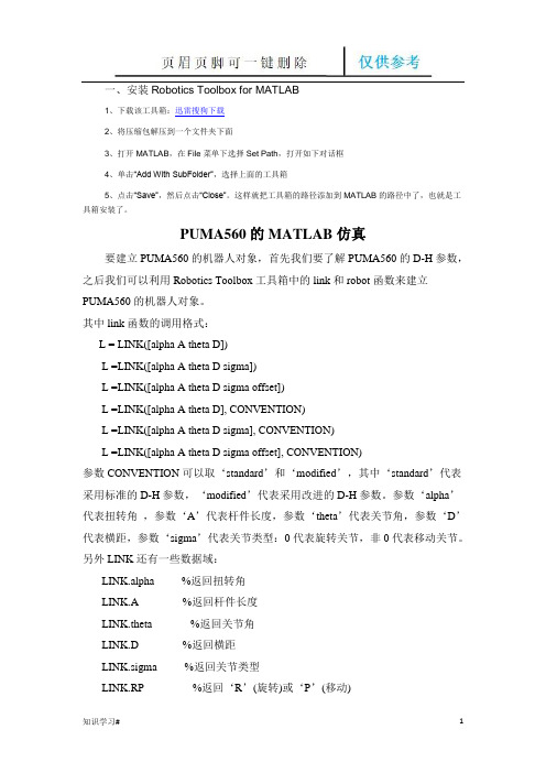
PUMA560的MATLAB仿真要建立PUMA560的机器人对象,首先我们要了解PUMA560的D-H参数,之后我们可以利用Robotics Toolbox工具箱中的link和robot函数来建立PUMA560的机器人对象。
其中link函数的调用格式:L = LINK([alpha A theta D])L =LINK([alpha A theta D sigma])L =LINK([alpha A theta D sigma offset])L =LINK([alpha A theta D], CONVENTION)L =LINK([alpha A theta D sigma], CONVENTION)L =LINK([alpha A theta D sigma offset], CONVENTION)参数CONVENTION可以取‘standard’和‘modified’,其中‘standard’代表采用标准的D-H参数,‘modified’代表采用改进的D-H参数。
参数‘alpha’代表扭转角,参数‘A’代表杆件长度,参数‘theta’代表关节角,参数‘D’代表横距,参数‘sigma’代表关节类型:0代表旋转关节,非0代表移动关节。
另外LINK还有一些数据域:LINK.alpha %返回扭转角LINK.A %返回杆件长度LINK.theta %返回关节角LINK.D %返回横距LINK.sigma %返回关节类型LINK.RP %返回‘R’(旋转)或‘P’(移动)LINK.mdh %若为标准D-H参数返回0,否则返回1LINK.offset %返回关节变量偏移LINK.qlim %返回关节变量的上下限[min max]LINK.islimit(q) %如果关节变量超限,返回-1, 0, +1LINK.I %返回一个3×3 对称惯性矩阵LINK.m %返回关节质量LINK.r %返回3×1的关节齿轮向量LINK.G %返回齿轮的传动比LINK.Jm %返回电机惯性LINK.B %返回粘性摩擦LINK.Tc %返回库仑摩擦LINK.dh return legacy DH rowLINK.dyn return legacy DYN row其中robot函数的调用格式:ROBOT %创建一个空的机器人对象ROBOT(robot) %创建robot的一个副本ROBOT(robot, LINK) %用LINK来创建新机器人对象来代替robotROBOT(LINK, ...) %用LINK来创建一个机器人对象ROBOT(DH, ...) %用D-H矩阵来创建一个机器人对象ROBOT(DYN, ...) %用DYN矩阵来创建一个机器人对象利用MATLAB中Robotics Toolbox工具箱中的transl、rotx、roty和rotz可以实现用齐次变换矩阵表示平移变换和旋转变换。
SCARA机器人MATLAB仿真实验过程考核3(仿真图+程序)

专业实践I 过程考核表程序:L1 = Link([0 0 32 0 0],'standard');L2 = Link([0 0 25 pi 0],'standard');L3 = Link([0 30 0 0 1],'standard');L3.qlim=[0,30];%行程限制L4 = Link([0 15 0 0 0],'standard');%D-H建模DHS = SerialLink([L1 L2 L3 L4]);%建立机器人连杆DHS.plotopt={'workspace',[-50 50 -50 50 -50 50]}; = 'SCARA';%命名qz=[pi,0,0,0];qr=[3/2*pi,-pi/3,20,pi];step=40;[q,qd,qdd] = jtraj(qz, qr, step);%该函数假定时间从0变到1,共经过M步。
它将轨迹返回到Q中,速度和加速度返回到QD和QDD中,它们都是MxN矩阵,%每个时间步长一行,每个joint一列。
Tc = fkine(DHS,q);%正运动变换矩阵qi = ikine(DHS,Tc,qz,[1 1 1 1 0 0]);%逆运动学求解ikine(机器人,变换矩阵,关节角度,六自由度以下用零隐藏)qq=qi(40,:)T = fkine(DHS,qi);%逆运动变换矩阵[qL,qdL,qddL] = jtraj(qz, qq, step);DHS.plot(q)DHS.plot(qi)figure%绘制位移、速度、加速度曲线%正运动学图像subplot(2,2,1);i=1:4;plot(q(:,i));title('位置');grid on;subplot(2,2,2);i=1:4;plot(qd(:,i));title('速度');grid on;subplot(2,2,3);i=1:4;plot(qdd(:,i));title('加速度');grid on;x = zeros(40,1);y = zeros(40,1);z = zeros(40,1);for j = 1:40x(j) = T(1,4,j);y(j) = T(2,4,j);z(j) = T(3,4,j);endsubplot(2,2,4)plot3(x,y,z,'b')title('运行轨迹')grid onfigure%绘制位移、速度、加速度曲线%逆运动学图像subplot(2,2,1);i=1:4;plot(qL(:,i));title('位置');grid on;subplot(2,2,2);i=1:4;plot(qdL(:,i));title('速度');grid on;subplot(2,2,3);i=1:4;plot(qddL(:,i));title('加速度');grid on;x = zeros(40,1);y = zeros(40,1);z = zeros(40,1);for j = 1:40x(j) = Tc(1,4,j);y(j) = Tc(2,4,j);z(j) = Tc(3,4,j);endsubplot(2,2,4)plot3(x,y,z,'b')title('运行轨迹')grid on。
基于Matlab的puma560型机器人仿真
基于MATLAB的puma560型机器人的仿真自121 成佳宇摘要:本文针对PUMA560型机器人,分析了它的正运动学、逆运动学和轨迹规划问题,并在MATLAB环境下,利用机器人仿真工具箱(Robotics Toolbox)对该机器人进行了建模。
同时仿真了正运动学和逆运动学求解和轨迹规划,并观察了各关节运动,得到所需的数据。
说明了所设计的参数是正确的,从而能够达到预定的目标。
关键字:puma560机器人;运动学;MATLAB Robotics Toolbox;仿真Abstract Based on PUMA560 robot, this article analyzes its forward kinematics and inverse kinematics and trajectory planning problem. and in the MATLAB environment, the robot simulation toolkit modeling for the robot. And simulation the forward kinematics and inverse kinematics and trajectory planning as well, observe the movement of each joint, we can get the required data. Shows the designed parameters are correct, so that they can reach a predetermined target. Keyword:PUMA560 robot;kinematics;MATLAB Robotics Toolbox;simulation引言机器人仿真利用计算机可视化和面向对象的手段,模拟机器人的动态特性,帮助研究人员了解机器人工作空间的形态及极限,揭示机构的合理的运动方案和控制算法,并在这台“机器人”上模拟能够实现的功能,使用户直接看到设计效果,及时找出缺点和不足,进行改进,从而解决在机器人设计、制造和运行过程中的问题,避免了直接操作实体可能造成的事故和不必要的损失,这将使机器人的研究和生产进入一个可预知的新时代。
matlab机器人工具箱matlabrobotics_toolbox_demo(共5则范文)
matlab机器人工具箱matlabrobotics_toolbox_demo(共5则范文)第一篇:matlab机器人工具箱matlabrobotics_toolbox_demo (共)MATLAB ROBOTTOOLrtdemo演示目录一、rtdemo机器人工具箱演示 (2)二、transfermations坐标转换 (2)三、Trajectory齐次方程 (8)四、forward kinematics 运动学正解 (12)四、Animation 动画 (18)五、Inverse Kinematics运动学逆解 (23)六、Jacobians雅可比---矩阵与速度 (32)七、Inverse Dynamics逆向动力学 (45)八、Forward Dynamics正向动力学 (52)一、rtdemo机器人工具箱演示 >> rtdemo %二、transfermations坐标转换% In the field of robotics there are many possible ways of representing% positions and orientations, but the homogeneous transformation is well% matched to MATLABs powerful tools for matrix manipulation.% % Homogeneous transformations describe the relationships between Cartesian% coordinate frames in terms of translation and orientation.% A pure translation of 0.5m in the X direction is represented bytransl(0.5, 0.0, 0.0)ans =1.00000.50001.00001.00001.0000 % % a rotation of 90degrees about the Y axis by roty(pi/2)ans =0.00001.00001.0000-1.00000.00001.0000 % % and a rotation of-90degrees about the Z axis by rotz(-pi/2)ans =0.00001.0000-1.00000.00001.00001.0000 % % these may be concatenated by multiplication t = transl(0.5, 0.0, 0.0)* roty(pi/2)* rotz(-pi/2)t =0.00000.00001.00000.5000-1.00000.0000-0.0000-1.00000.00001.0000% % If this transformation represented the origin of a new coordinate frame with respect % to the world frame origin(0, 0, 0), that new origin would be given byt * [0 0 0 1]' ans =0.50001.0000pause % any key to continue % % the orientation of the new coordinate frame may be expressed in terms of % Euler angles tr2eul(t)ans =1.5708-1.5708 % % or roll/pitch/yaw anglestr2rpy(t)ans =-1.57080.0000-1.5708pause % any key to continue % % It is important to note that tranform multiplication is in general not% commutative as shown by the following examplerotx(pi/2)* rotz(-pi/8)ans =0.92390.3827-0.00000.0000-1.0000-0.38270.92390.0000rotz(-pi/8)* rotx(pi/2)ans =0.92390.0000-0.3827-0.38270.0000-0.92391.00000.0000% % pause % any key to continue echo off 1.00000 1.0000三、Trajectory齐次方程% The path will move the robot from its zero angle pose to the upright(or % READY)pose.% % First create a time vector, completing the motion in 2 seconds with a % sample interval of 56ms.t = [0:.056:2];pause % hit any key to continue % % A polynomial trajectory between the 2 poses is computed using jtraj()%q = jtraj(qz, qr, t);pause % hit any key to continue % % For this particular trajectory most of the motion is done by joints 2 and 3, % and this can be conveniently plotted using standard MATLAB operationssubplot(2,1,1)plot(t,q(:,2))title('Theta')xlabel('Time(s)');ylabel('Joint 2(rad)')subplot(2,1,2)plot(t,q(:,3))xlabel('Time(s)');ylabel('Joint 3(rad)')pause % hit any key to continue% % We can also look at the velocity and acceleration profiles.We could% differentiate the angle trajectory using diff(), but more accurate results% can be obtained by requesting that jtraj()return angular velocity and% acceleration as follows[q,qd,qdd] = jtraj(qz, qr, t);% % which can then be plotted asbeforesubplot(2,1,1)plot(t,qd(:,2))title('Velocity')xlabel('Time(s)');ylabel('Joint 2 vel(rad/s)')subplot(2,1,2)plot(t,qd(:,3))xlabel('Time(s)');ylabel('Joint 3 vel(rad/s)')pause(2)% and the joint acceleration profilessubplot(2,1,1)plot(t,qdd(:,2))title('Acceleration')xlabel('Time(s)');ylabel('Joint 2 accel(rad/s2)')subplot(2,1,2)plot(t,qdd(:,3))xlabel('Time(s)');ylabel('Joint 3 accel(rad/s2)')pause % any key to continueecho off四、forward kinematics 运动学正解% Forward kinematics is the problem of solving the Cartesian position and% orientation of a mechanism given knowledge of the kinematic structure and % the joint coordinates.% % Consider the Puma 560 example again, and the joint coordinates of zero, % which are defined by qzqz qz =0 % % The forward kinematics may be computed using fkine()with an appropropriate% kinematic description, in this case, the matrix p560 which defines% kinematics for the 6-axis Puma 560.fkine(p560, qz)ans =1.00000.45211.0000-0.15001.00000.43181.0000 % % returns the homogeneous transform corresponding to the last link of the % manipulator pause % any key to continue % % fkine()can also be used with a time sequence of joint coordinates, or% trajectory, which is generated by jtraj()%t = [0:.056:2];% generate a time vectorq = jtraj(qz, qr, t);% compute the joint coordinate trajectory % % then the homogeneous transform for each set of joint coordinates is given byT = fkine(p560, q);% % where T is a 3-dimensional matrix, the first two dimensions are a 4x4% homogeneous transformation and the third dimension is time.% % For example, the first point isT(:,:,1)ans =1.00001.00000 % % and the tenth point isT(:,:,10)ans =1.0000-0.0000-0.00001.00000 0.4521-0.1500 0.43181.0000 0.4455-0.1500 0.50681.00001.00001.0000pause % any key to continue % % Elements(1:3,4)correspond to the X, Y and Z coordinates respectively, and% may be plotted against timesubplot(3,1,1)plot(t, squeeze(T(1,4,:)))xlabel('Time(s)');ylabel('X(m)')subplot(3,1,2)plot(t, squeeze(T(2,4,:)))xlabel('Time(s)');ylabel('Y(m)')subplot(3,1,3)plot(t, squeeze(T(3,4,:)))xlabel('Time(s)');ylabel('Z(m)')pause % any key to continue %% or we could plot X against Z to get some idea of the Cartesian path followed % by the manipulator.%subplot(1,1,1)plot(squeeze(T(1,4,:)), squeeze(T(3,4,:)));xlabel('X(m)')ylabel('Z(m)')grid pause % any key to continueecho off四、Animation 动画 clf % % The trajectory demonstration has shown how a joint coordinate trajectory % may be generatedt = [0:.056:2]';% generate a time vectorq = jtraj(qz, qr, t);% generate joint coordinate trajectory % % the overloaded function plot()animates a stick figure robot moving% along a trajectory.plot(p560, q);% The drawn line segments do not necessarily correspond to robot links, but % join the origins of sequential link coordinate frames.% % A small right-angle coordinate frame is drawn on the end of the robot to show % the wrist orientation.% % A shadow appears on the ground which helps to give some better idea of the % 3D object.pause % any key to continue% % We can also place additional robots into a figure.% % Let's make a clone of the Puma robot, but change its name and base locationp560_2 = p560;p560_ = 'another Puma';p560_2.base = transl(-0.5, 0.5, 0);hold onplot(p560_2, q);pause % any key to continue% We can also have multiple views of the same robotclfplot(p560, qr);figureplot(p560, qr);view(40,50)plot(p560, q)pause % any key to continue% % Sometimes it's useful to be able to manually drive the robot around to % get an understanding of how it works.drivebot(p560)%% use the sliders to control the robot(in fact both views).Hitthe red quit % button when you are done.echo off五、Inverse Kinematics运动学逆解% % Inverse kinematics is the problem of finding the robot joint coordinates, % given a homogeneous transform representing the last link of the manipulator.% It is very useful when the path is planned in Cartesian space, for instance % a straight line path as shown in the trajectory demonstration.% % First generate the transform corresponding to a particular joint coordinate,q = [0-pi/4-pi/4 0 pi/8 0] q =-0.7854-0.78540.3927T = fkine(p560, q);% % Now the inverse kinematic procedure for any specific robot can be derived% symbolically and in general an efficient closed-form solution can be% obtained.However we are given only a generalized description of the% manipulator in terms of kinematic parameters so an iterative solution will% be used.The procedure is slow, and the choice of starting value affects% search time and the solution found, since in general a manipulator may% have several poses which result in the same transform for the last % link.The starting point for the first point may be specified, or else it % defaults to zero(which is not a particularlygood choice in this case)qi = ikine(p560, T);qi' ans =-0.0000-0.7854-0.7854-0.00000.39270.0000 % % Compared with the original valueq q =-0.7854-0.78540.39270 % % A solution is not always possible, for instance if the specified transform% describes a point out of reach of the manipulator.As mentioned above% the solutions are not necessarily unique, and there are singularities% at which the manipulator loses degrees of freedom and joint coordinates% become linearly dependent.pause % any key to continue % % T o examine the effect at a singularity lets repeat the last example but for a % different pose.At the `ready' position two of the Puma's wrist axes are% aligned resulting in the loss of one degree of freedom.T = fkine(p560, qr);qi = ikine(p560, T);qi' ans =-0.00001.5238-1.4768-0.0000-0.04700.0000 % % which is not the same as the original joint angleqr qr =1.5708-1.5708pause % any key to continue % % However both result in the same end-effector positionfkine(p560, qi)-fkine(p560, qr)ans =1.0e-015 *-0.0000-0.0902-0.06940.0000-0.00000.09020.00000.1110pause % any key to continue% Inverse kinematics may also be computed for a trajectory.% If we take a Cartesian straight line patht = [0:.056:2];% create a time vectorT1 = transl(0.6,-0.5, 0.0)% define the start point T1 =1.00000.60001.0000-0.50001.00001.0000T2 = transl(0.4, 0.5, 0.2)% and destination T2 =1.00000.40001.00000.50001.00000.20001.0000T = ctraj(T1, T2, length(t));% compute a Cartesian path % % now solve the inverse kinematics.When solving for a trajectory, the% starting joint coordinates for each point is taken as the result of the% previous inverse solution.%ticq = ikine(p560, T);toc Elapsed time is 0.315656 seconds.% % Clearly this approach is slow, and not suitable for a real robot controller % where an inverse kinematic solution would be required in a few milliseconds.% % Let's examine the joint space trajectory that results in straightline % Cartesian motionsubplot(3,1,1)plot(t,q(:,1))xlabel('Time(s)');ylabel('Joint 1(rad)')subplot(3,1,2)plot(t,q(:,2))xlabel('Time(s)');ylabel('Joint 2(rad)')subplot(3,1,3)plot(t,q(:,3))xlabel('Time(s)');ylabel('Joint 3(rad)')pause % hit any key to continue% This joint space trajectory can now be animatedplot(p560, q)pause % any key to continueecho off %六、Jacobians雅可比---矩阵与速度% Jacobian and differential motion demonstration % % A differential motion can be represented by a 6-element vector with elements % [dx dy dz drx dry drz] % % where the first 3 elements are a differential translation, and the last 3 % are a differential rotation.When dealing with infinitisimal rotations,% the order becomes unimportant.The differential motion could be written% in terms of compounded transforms % % transl(dx,dy,dz)* rotx(drx)* roty(dry)* rotz(drz)% % but a more direct approach is to use the function diff2tr()%D = [.1.2 0-.2.1.1]';diff2tr(D)ans =-0.10000.10000.10000.10000.20000.2000-0.1000-0.2000pause % any key to continue % % More commonly it is useful to know how a differential motion in one% coordinate frame appears in another frame.If the second frame is% represented by the transformT = transl(100, 200, 300)* roty(pi/8)* rotz(-pi/4);% % then the differential motion in the second frame would be given by DT = tr2jac(T)* D;DT' ans =-29.510969.7669-42.3289-0.2284-0.08700.0159 % % tr2jac()has computed a 6x6 Jacobian matrix which transforms the differential% changes from the first frame to the next.% pause % any key to continue% The manipulator's Jacobian matrix relates differential joint coordinate% motion to differential Cartesian motion;% % dX = J(q)dQ % % For an n-joint manipulator the manipulator Jacobian is a 6 x n matrix and % is used is many manipulator control schemes.For a 6-axis manipulator like % the Puma 560 the Jacobian is square % % Two Jacobians are frequently used, which express the Cartesian velocity in % the world coordinate frame,q = [0.1 0.75-2.25 0.75 0] q =0.10000.7500-2.25000.7500J = jacob0(p560, q)J =0.0746-0.3031-0.0102 00.7593-0.0304-0.0010 00.74810.4322 00.00000.09980.0998 0.6782-0.9950-0.9950 0.06811.00000.00000.0000 0.7317 % % or the T6 coordinate frame J = jacobn(p560, q)0 0.9925 0.0996 0.07070 0.0998-0.9950 0.0000J =0.1098-0.7328-0.30210.74810.00000.00000.10230.33970.3092-0.68160.6816-0.0000-1.0000-1.0000-0.0000-1.00000.73170.00000.00000.73170.00001.0000 % % Note the top right 3x3 block is all zero.This indicates, correctly, that % motion of joints 4-6 does not cause any translational motion of the robot's % end-effector.pause % any key to continue % % Many control schemes require the inverse of the Jacobian.The Jacobian % in this example is not singulardet(J)ans =-0.0632 % % and may be invertedJi = inv(J)Ji =0.00001.3367-0.0000 0-2.49460.6993-2.4374 00.0000-0.0000 0.0000-0.00002.7410-1.21065.91250.00000.00000.00001.3367-0.00001.4671-0.0000-0.24640.5113-3.4751-0.0000-1.0000-0.0000-1.95610.0000-1.07340.00001.0000pause % any key to continue % % A classic control technique is Whitney's resolved rate motion control % % dQ/dt = J(q)^-1 dX/dt % % where dX/dt is the desired Cartesian velocity, and dQ/dt is the required % joint velocity to achieve this.vel = [1 0 0 0 0 0]';% translational motion in the X directionqvel = Ji * vel;qvel' ans =0.0000-2.49462.74100.0000-0.2464-0.0000 % % This is an alternative strategy to computing a Cartesian trajectory% and solving the inverse kinematics.However like that other scheme, this % strategy also runs into difficulty at a manipulator singularity where % the Jacobian is singular.pause % any key to continue % % As already stated this Jacobian relates joint velocity to end-effector% velocity expressed in the end-effector reference frame.We may wish% instead to specify the velocity in base or world coordinates.% % We have already seen how differential motions in one frame can be translated% to another.Consider the velocity as a differential in the world frame, that % is, d0X.We can write % d6X = Jac(T6)d0X % T6 = fkine(p560, q);% compute the end-effector transform d6X = tr2jac(T6)* vel;% translate world frame velocity to T6 frameqvel = Ji * d6X;% compute required joint velocity as before qvel' ans =-0.1334-3.53916.1265-0.1334-2.58740.1953 % % Note that this value of joint velocity is quite different to that calculated % above, which was for motion in the T6 X-axis direction.pause % any key to continue % % At a manipulator singularity or degeneracy the Jacobian becomes singular.% At the Puma's `ready' position for instance, two of the wrist joints are % aligned resulting in the loss of one degree of freedom.This is revealed by % the rank of the Jacobian rank(jacobn(p560, qr))ans = % % and the singular values are svd(jacobn(p560, qr))ans =1.90661.73210.56600.01660.00810.0000pause % any key to continue % % When not actually at a singularity the Jacobian can provide information% about how `well-conditioned' the manipulator is for making certain motions, % and is referred to as `manipulability'.% % A number of scalar manipulability measures have been proposed.One by % Yoshikawamaniplty(p560, q, 'yoshikawa')ans =[] % % is based purely on kinematic parameters of the manipulator.% % Another by Asada takes into account the inertia of the manipulator which% affects the acceleration achievable in different directions.This measure% varies from 0 to 1, where 1 indicates uniformity of acceleration in all % directionsmaniplty(p560, q, 'asada')ans =[] % % Both of these measures would indicate that this particular pose is not well % conditioned.pause % any key to continue% An interesting class of manipulators are those that are redundant, that is, % they have more than 6 degrees of puting the joint motion for % such a manipulator is not straightforward.Approaches have been suggested % based on the pseudo-inverse of the Jacobian(which will not be square)or % singular value decomposition of the Jacobian.% echo off七、Inverse Dynamics逆向动力学% % Inverse dynamics computes the joint torques required to achieve the specified % state of joint position, velocity and acceleration.% The recursive Newton-Euler formulation is an efficient matrix oriented % algorithm for computing the inverse dynamics, and is implemented in the % function rne().% % Inverse dynamics requires inertial and mass parameters of each link, as well % as the kinematic parameters.This is achieved by augmenting the kinematic% description matrix with additional columns for the inertial and mass% parameters for each link.% % For example, for a Puma 560 in the zero angle pose, with all joint velocities % of 5rad/s and accelerations of 1rad/s/s, the joint torques required are % tau = rne(p560, qz, 5*ones(1,6), ones(1,6))tau =-79.404837.169413.54551.07280.93990.5119pause % any key to continue% As with other functions the inverse dynamics can be computed for each point% on a trajectory.Create a joint coordinate trajectory and compute velocity % and acceleration as wellt = [0:.056:2];% create time vector[q,qd,qdd] = jtraj(qz, qr, t);% compute joint coordinate trajectorytau = rne(p560, q, qd, qdd);% compute inverse dynamics % % Now the joint torques can be plotted as a function of time plot(t, tau(:,1:3))xlabel('Time(s)');ylabel('Joint torque(Nm)')pause % any key to continue% % Much of the torque on joints 2 and 3 of a Puma 560(mounted conventionally)is % due to gravity.That component can be computed using gravload()taug = gravload(p560, q);plot(t, taug(:,1:3))xlabel('Time(s)');ylabel('Gravity torque(Nm)')pause % any key to continue% Now lets plot that as a fraction of the total torque required over the % trajectorysubplot(2,1,1)plot(t,[tau(:,2)taug(:,2)])xlabel('Time(s)');ylabel('Torque on joint 2(Nm)')subplot(2,1,2)plot(t,[tau(:,3)taug(:,3)])xlabel('Time(s)');ylabel('Torque on joint 3(Nm)')pause % any key to continue% % The inertia seen by the waist(joint 1)motor changes markedly with robot% configuration.The function inertia()computes the manipulator inertia matrix % for any given configuration.% % Let's compute the variation in joint 1 inertia, that is M(1,1), as the % manipulator moves along the trajectory(this may take a few minutes)M = inertia(p560, q);M11 = squeeze(M(1,1,:));plot(t, M11);xlabel('Time(s)');第二篇:matlab的nntool工具箱小结拟合以及插值还有逼近是数值分析的三大基础工具,通俗意义上它们的区别在于:拟合是已知点列,从整体上靠近它们;插值是已知点列并且完全经过点列;逼近是已知曲线,或者点列,通过逼近使得构造的函数无限靠近它们。
MATLAB机器人仿真程序
MATLAB机器人仿真程序随着机器人技术的不断发展,机器人仿真技术变得越来越重要。
MATLAB是一款强大的数学计算软件,也被广泛应用于机器人仿真领域。
本文将介绍MATLAB在机器人仿真程序中的应用。
一、MATLAB简介MATLAB是MathWorks公司开发的一款商业数学软件,主要用于算法开发、数据可视化、数据分析以及数值计算等。
MATLAB具有丰富的工具箱,包括信号处理、控制系统、神经网络、图像处理等,可以方便地实现各种复杂的计算和分析。
二、MATLAB机器人仿真程序在机器人仿真领域,MATLAB可以通过Robotics System Toolbox实现各种机器人的仿真。
该工具箱包含了机器人运动学、动力学、控制等方面的函数库,可以方便地实现机器人的建模、控制和可视化。
下面是一个简单的MATLAB机器人仿真程序示例:1、建立机器人模型首先需要定义机器人的几何参数、连杆长度、质量等参数,并使用Robotics System Toolbox中的函数建立机器人的运动学模型。
例如,可以使用robotics.RigidBodyTree函数来建立机器人的刚体模型。
2、机器人运动学仿真在建立机器人模型后,可以使用Robotics System Toolbox中的函数进行机器人的运动学仿真。
例如,可以使用robotics.Kinematics函数计算机器人的位姿,并使用robotics.Plot函数将机器人的运动轨迹可视化。
3、机器人动力学仿真除了运动学仿真外,还可以使用Robotics System Toolbox中的函数进行机器人的动力学仿真。
例如,可以使用robotics.Dynamic函数计算机器人在给定速度下的加速度和力矩,并使用robotics.Plot函数将机器人的运动轨迹可视化。
4、机器人控制仿真可以使用Robotics System Toolbox中的函数进行机器人的控制仿真。
例如,可以使用robotics.Controller函数设计机器人的控制器,并使用robotics.Plot函数将机器人的运动轨迹可视化。
matlab仿真工具 基本操作

matlab仿真工具基本操作Matlab是一种功能强大的数学仿真工具,它提供了丰富的功能和工具箱,可以用于各种科学计算、数据分析和模型仿真等领域。
本文将介绍Matlab仿真工具的基本操作,帮助读者快速上手使用该工具。
一、Matlab的安装与启动在开始使用Matlab之前,首先需要将其安装在计算机上。
用户可以从MathWorks官方网站下载Matlab的安装程序,并按照安装向导进行操作。
安装完成后,可以通过桌面上的快捷方式或者在命令行中输入"matlab"来启动Matlab。
二、Matlab的界面与基本操作Matlab的界面由多个窗口组成,包括命令窗口、编辑器窗口、工作空间窗口、命令历史窗口等。
用户可以通过菜单栏、工具栏或者命令行来执行各种操作。
1. 命令窗口:用户可以在命令窗口中直接输入Matlab命令,并按下Enter键执行。
Matlab会立即给出相应的结果,并显示在命令窗口中。
2. 编辑器窗口:用户可以在编辑器窗口中编写Matlab脚本文件,以便进行更复杂的操作。
脚本文件可以保存为.m文件,并通过命令窗口中的"run"命令或者点击编辑器窗口中的运行按钮来执行。
3. 工作空间窗口:工作空间窗口显示了当前Matlab工作空间中的变量列表。
用户可以通过命令行或者脚本文件来创建、修改和删除变量,并在工作空间窗口中查看其值和属性。
4. 命令历史窗口:命令历史窗口记录了用户在命令窗口中输入的所有命令,方便用户查找和重复使用。
三、Matlab的数学计算功能Matlab提供了丰富的数学计算函数,可以进行向量和矩阵运算、符号计算、微积分、线性代数、概率统计等操作。
用户可以通过命令行或者脚本文件来调用这些函数,并进行各种数学计算。
1. 向量和矩阵运算:Matlab中可以方便地定义和操作向量和矩阵。
用户可以使用矩阵运算符(如+、-、*、/)对向量和矩阵进行加减乘除等运算,还可以使用内置函数(如transpose、inv、det)进行转置、求逆和求行列式等操作。
- 1、下载文档前请自行甄别文档内容的完整性,平台不提供额外的编辑、内容补充、找答案等附加服务。
- 2、"仅部分预览"的文档,不可在线预览部分如存在完整性等问题,可反馈申请退款(可完整预览的文档不适用该条件!)。
- 3、如文档侵犯您的权益,请联系客服反馈,我们会尽快为您处理(人工客服工作时间:9:00-18:30)。
附录
MATLAB
机器人工具箱仿真程序:
1)运动学仿真模型程序(Rob1.m)
L1=link([pi/2 150 0 0])
L2=link([0 570 0 0])
L3=link([pi/2 130 0 0])
L4=link([-pi/2 0 0 640])
L5=link([pi/2 0 0 0])
L6=link([0 0 0 95])
r=robot({L1 L2 L3 L4 L5 L6})
=’MOTOMAN-UP6’ % 模型的名称
>>drivebot(r)
2)正运动学仿真程序(Rob2.m)
L1=link([pi/2 150 0 0])
L2=link([0 570 0 0])
L3=link([pi/2 130 0 0])
L4=link([-pi/2 0 0 640])
L5=link([pi/2 0 0 0])
L6=link([0 0 0 95])
r=robot({L1 L2 L3 L4 L5 L6})
=
’MOTOMAN-UP6’
t=[0:0.01:10];%产生时间向量
qA=[0 0 0 0 0 0 ]; %机械手初始关节角度
qAB=[-pi/2 -pi/3 0 pi/6 pi/3 pi/2 ];%机械手终止关节角度
figure('Name','up6机器人正运动学仿真演示');%给仿真图像命名q=jtraj(qA,qAB,t);%生成关节运动轨迹
T=fkine(r,q);%正向运动学仿真函数
plot(r,q);%生成机器人的运动
figure('Name','up6机器人末端位移图')
subplot(3,1,1);
plot(t, squeeze(T(1,4,:))); xlabel('Time (s)'); ylabel('X (m)'); subplot(3,1,2); plot(t, squeeze(T(2,4,:))); xlabel('Time (s)'); ylabel('Y (m)'); subplot(3,1,3); plot(t, squeeze(T(3,4,:))); xlabel('Time (s)'); ylabel('Z (m)');
x=squeeze(T(1,4,:)); y=squeeze(T(2,4,:)); z=squeeze(T(3,4,:));
figure('Name','up6机器人末端轨迹图'); plot3(x,y,z);
3)机器人各关节转动角度仿真程序:(Rob3.m)
L1=link([pi/2 150 0 0 ])
L2=link([0 570 0 0])
L3=link([pi/2 130 0 0])
L4=link([-pi/2 0 0 640])
L5=link([pi/2 0 0 0 ])
L6=link([0 0 0 95])
r=robot({L1 L2 L3 L4 L5 L6})
='motoman-up6'
t=[0:0.01:10];
qA=[0 0 0 0 0 0 ];
qAB=[ pi/6 pi/6 pi/6 pi/6 pi/6 pi/6];
q=jtraj(qA,qAB,t);
Plot(r,q); subplot(6,1,1);
plot(t,q(:,1)); title('转动关节1');
xlabel('时间/s'); ylabel('角度/rad');
subplot(6,1,2); plot(t,q(:,2));
title('转动关节2'); xlabel('时间/s'); ylabel('角度/rad');
subplot(6,1,3); plot(t,q(:,3));
title('转动关节3'); xlabel('时间/s'); ylabel('角度/rad');
subplot(6,1,4); plot(t,q(:,4));
title('转动关节4'); xlabel('时间/s'); ylabel('角度/rad' );
subplot(6,1,5); plot(t,q(:,5));
title('转动关节5'); xlabel('时间/s'); ylabel('角度/rad');
subplot(6,1,6); plot(t,q(:,6));
title('转动关节6'); xlabel('时间/s'); ylabel('角度/rad');
4)机器人各关节转动角速度仿真程序:(Rob4.m)
t=[0:0.01:10];
qA=[0 0 0 0 0 0 ];%机械手初始关节量
qAB=[ 1.5709 -0.8902 -0.0481 -0.5178 1.0645 -1.0201];
[q,qd,qdd]=jtraj(qA,qAB,t);
Plot(r,q); subplot(6,1,1); plot(t,qd(:,1));
title('转动关节1'); xlabel('时间/s'); ylabel('rad/s');
subplot(6,1,2); plot(t,qd(:,2));
title('转动关节2'); xlabel('时间/s'); ylabel('rad/s'); subplot(6,1,3); plot(t,qd(:,3));
title('转动关节3'); xlabel('时间/s'); ylabel('rad/s'); subplot(6,1,4); plot(t,qd(:,4));
title('转动关节4'); xlabel('时间/s'); ylabel('rad/s' ); subplot(6,1,5); plot(t,qd(:,5));
title('转动关节5'); xlabel('时间/s'); ylabel('rad/s'); subplot(6,1,6); plot(t,qd(:,6));
title('转动关节6'); xlabel('时间/s'); ylabel('rad/s');
5)机器人各关节转动角加速度仿真程序:(Rob5.m)
t=[0:0.01:10];%产生时间向量
qA=[0 0 0 0 0 0]
qAB =[1.5709 -0.8902 -0.0481 -0.5178 1.0645 -1.0201]; [q,qd,qdd]=jtraj(qA,qAB,t);
figure('name','up6机器人机械手各关节加速度曲线');
subplot(6,1,1); plot(t,qdd(:,1));
title('关节1'); xlabel('时间 (s)'); ylabel('加速度 (rad/s^2)'); subplot(6,1,2); plot(t,qdd(:,2));
title('关节2'); xlabel('时间 (s)'); ylabel('加速度 (rad/s^2)'); subplot(6,1,3); plot(t,qdd(:,3));
title('关节3'); xlabel('时间 (s)'); ylabel('加速度 (rad/s^2)') subplot(6,1,4); plot(t,qdd(:,4));
title('关节4'); xlabel('时间 (s)'); ylabel('加速度 (rad/s^2)') subplot(6,1,5); plot(t,qdd(:,5));
title('关节5'); xlabel('时间 (s)'); ylabel('加速度 (rad/s^2)')
subplot(6,1,6); plot(t,qdd(:,6));
title('关节6'); xlabel('时间 (s)'); ylabel('加速度 (rad/s^2)')。