XFlow 2015 tutorials users guide 含13个例子的全部教程
xflow_2012学习资料(三)固体运动方式定义
Xflow_2012自编学习(三)固体运动方式XFlow_2012能够处理大规模复杂模型,并且结合移动部分、强制或关联运动或接触建模过程,极大地简化分析结构。
Xflow_2012中针对几何对象的运动过程模拟,提供4中类型运动定义方式。
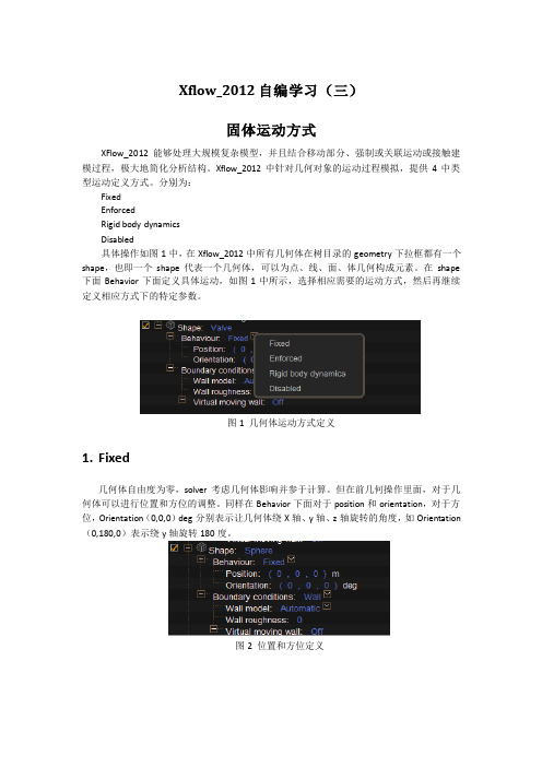
分别为:FixedEnforcedRigid body dynamicsDisabled具体操作如图1中,在Xflow_2012中所有几何体在树目录的geometry下拉框都有一个shape,也即一个shape代表一个几何体,可以为点、线、面、体几何构成元素。
在shape 下面Behavior下面定义具体运动,如图1中所示,选择相应需要的运动方式,然后再继续定义相应方式下的特定参数。
图1 几何体运动方式定义1.Fixed几何体自由度为零,solver考虑几何体影响并参于计算。
但在前几何操作里面,对于几何体可以进行位置和方位的调整。
同样在Behavior下面对于position和orientation,对于方位,Orientation(0,0,0)deg分别表示让几何体绕X轴、y轴、z轴旋转的角度,如Orientation (0,180,0)表示绕y轴旋转180度。
图2 位置和方位定义2.Enforced此类型几何体运动方式定义就是指定运动规律,同时包括位置和角速度两种方式,对于角速度方式,对应两种模式,一是Euler angles欧拉角度,二是Axis angles轴角度。
Euler angles 为指定几何体绕笛卡尔坐标轴旋转动作行为,只需输入绕X、Y、Z轴的角速度;Axis angles 为指定几何体绕任意坐标轴旋转动作,需要输入轴方向和角速度。
其次就是指定位置的定义方式相对比较简单,给定X、Y、Z方向的运动方式。
此两种方式的函数表达式中,可以有效调用的函数变量只能为时间t,即都只能为时间的函数,物理学讲即为运动方程S=S(t)、A=A(t)。
具体设置情况如图3中图3 指定几何体运动方程3.Rigid body dynamics在Xflow_2012中采用rigid body dynamics时,几何体被视为刚体,定义刚体运动方式的六自由度被激活,如X、Y、Z方向上的位置,X、Y、Z矢量轴上旋转,同时每个自由度还可以受到外力或外部动量约束。
makeFlow 1.0.2 软件说明书
Package‘makeFlow’October13,2022Type PackageTitle Visualizing Sequential ClassificationsVersion1.0.2Date2016-08-22Author Alex J.KrebsMaintainer Alex J.Krebs<*********************>Description A user-friendly tool for visualizing categorical or group movement. License GPL(>=2)Imports dplyr,RColorBrewerCopyright Copyright Notice GENERAL DISCLAIMER This program is free software;you can redistribute it and/or modify it under theterms of the GNU General Public License as published by theFree Software Foundation;either version2,or(at your option)any later version.This program is distributed in the hope thatit will be useful,but WITHOUT ANY W ARRANTY;without even theimplied warranty of MERCHANTABILITY or FITNESS FOR A PARTICULAR PURPOSE.See the GNU General Public License for more details.In short:You may use it any way you like,as long as you donot charge money for it,remove this notice,or hold anyoneliable for its results.Also,please acknowledge the source andcommunicate changes to the author.If this software is used inwork presented for publication,kindly reference it using forexample:Krebs AJ(2016):makeFlow:Visualizing SequentialClassifications.Be sure to reference R itself and otherlibraries used.RoxygenNote5.0.1NeedsCompilation noRepository CRANDate/Publication2016-08-2418:02:3812makeFlow-packageR topics documented:makeFlow-package (2)addAlpha (3)colorCount (4)FlowSummaries (5)GateSummaries (6)makeFlow (7)shelters (9)Index10 makeFlow-package Visualizing Sequential ClassificationsDescriptionA user-friendly tool for visualizing categorical or group movement.DetailsThe DESCRIPTIONfile:Package:makeFlowType:PackageTitle:Visualizing Sequential ClassificationsVersion: 1.0.2Date:2016-08-22Author:Alex J.KrebsMaintainer:Alex J.Krebs<*********************>Description:A user-friendly tool for visualizing categorical or group movement.License:GPL(>=2)Imports:dplyr,RColorBrewerCopyright:Copyright Notice GENERAL DISCLAIMER This program is free software;you can redistribute it and/or mo RoxygenNote: 5.0.1Index of help topics:FlowSummaries FlowSummaries()GateSummaries GateSummaries()addAlpha addAlpha()colorCount colorCount()makeFlow makeFlow()makeFlow-package Visualizing Sequential Classificationsshelters sheltersUsers should ensure all classFields(columns)are explicitly defined in the same dataset.color-Count(),FlowSummaries(),GateSummaries(),and makeFlow()can all operate with the same twoaddAlpha3 basic inputs:data and classFields.Graphical parameters can be defined with additional makeFlow() arguments.Author(s)Alex J.KrebsMaintainer:Alex J.Krebs<*********************>Examples##Data:##carData<-mtcars##carData$car<-"All Cars"##carData$speedclass<-ifelse(carData$qsec<15,"Fast",##ifelse(carData$qsec<18,"Mid-Speed","Slow"))##carData$speedclass<-factor(x=carData$speedclass,levels=c("Slow","Mid-Speed","Fast")) ####Create Diagram:##makeFlow(data=carData,classFields=c("car","cyl","speedclass"),##gateWidth=20,minVerticalBtwnGates=.15,distanceBtwnGates=70,##fieldLabels=c("","Cylinders","Speed"),gateBorder="black")##Generate underlying tables using GateSummaries()and FlowSummaries()addAlpha addAlpha()DescriptionAdds a specified opacity(between0and1)to any color(s)listed.UsageaddAlpha(col,alpha=1)Argumentscol A vector of one or many colors.alpha A value between0and1.0indicates complete transparency.1indicates com-plete opacity.ValueReturns the Hexadecimal representation of the modified color(s).4colorCount Examples##The function is currently defined asfunction(col,alpha=1){if(missing(col))stop("Please provide a vector of colors.")apply(sapply(col,col2rgb)/255,2,function(x){rgb(x[1],x[2],x[3],alpha=alpha)})}colorCount colorCount()DescriptionReturns an integer representing the number of unique categories from all specifiedfields.This value should serve as a guide for users specifying colors in the makeFlow()function.UsagecolorCount(data,classFields)Argumentsdata An object of class data.frame in which all specified classFields(or column names)can be found.classFields A vector of the column names intended to be represented in a makeFlow()dia-gram.Each element must be a string.NoteRelies on Hadley Wickham’s dplyr package.Author(s)Alex J.KrebsFlowSummaries5 FlowSummaries FlowSummaries()DescriptionOutputs a list of objects of class tbl_df containing values presented in a makeFlow()diagram utiliz-ing the same data and classFields arguments.UsageFlowSummaries(data,classFields)Argumentsdata An object of class data.frame in which all specified classFields(column names)can be found.classFields A vector of the column names intended to be represented in the makeFlow()diagram.Each element must be a string.DetailsOutputs tables with standard naming convention of Flow_Summary_x.For example,Flow_Summary_1 provides the counts and frequencies of each category(gate)from thefirst column specified in class-Fields moving to each of the categories(gates)in the second column listed in classFields.NoteRelies on Hadley Wickham’s dplyr package.Author(s)Alex J.KrebsExamples##myFlows<-FlowSummaries(data=shelters,classFields=c("loc","Jan","Feb","Mar"))##Flow_Summary_2will show the counts and percentages from##"Jan"categories that move to the categories in"Feb"6GateSummaries GateSummaries GateSummaries()DescriptionOutputs a list of objects of class tbl_df containing the values in a makeFlow()diagram utilizing the same data and classFields arguments.UsageGateSummaries(data,classFields)Argumentsdata An object of class data.frame in which all specified classFields(column names)can be found.classFields A vector of the column names intended to be represented in a makeFlow()dia-gram.Each element must be a string.DetailsOutputs tables with standard naming convention of Gate_Summary_x.For example,Gate_Summary_1 provides the counts and frequencies of each category within thefirst column specified in the class-Fields argument.NoteRelies on Hadley Wickham’s dplyr package.Author(s)Alex J.KrebsExamples##myGates<-GateSummaries(data=shelters,classFields=c("loc","Jan","Feb","Mar")) ##Gate_Summary_2will show the count and percentage of observations##within each category of the column"Jan"makeFlow makeFlow()DescriptionUses the selected dataset and specified order of columns to produce a left-to-rightflow diagram.This function assumes the use of a single dataset and categorical variables resembling observations’movement from one state to another,such that at every state,every observation can be mapped.Colors bridging states assume the color of the gate from which they originate.UsagemakeFlow(data,classFields,rotate=F,gatecolors=NA,minVerticalBtwnGates=0.1, connectingAlpha=0.5,bg="white",plotTitle="",titleAdj=0.5,txtColor="black", distanceBtwnGates=50,gateWidth=7,gateBorder=NA,labels=T,fieldLabels=NA, showPercentages=T,showConnectPercentages=F,percentTextColor="black",showCounts=T,countTextColor="black")Argumentsdata An object of class data.frame in which all specified classFields(column names)can be found.classFields A vector of the column names intended to be represented in a makeFlow()dia-gram.Each element in this vector must be a string.rotate Set to TRUE to rotate all text.This is a work-around to allow for a vertical(top-down)flow.Manual manipulation after exporting a diagram is needed to adjustthe orientation of the output.gatecolors A vector of colors to apply to gates.For greater control,the alphabetized orderof categories from all selected classFields will match the corresponding colorin this list.If the length of this vector is shorter than the number of uniquecategories in the full diagram,a predefined palette"Set3"is substituted in itsplace,and a warning message will alert the user of how many colors are requiredfor manual input.If more colors are supplied than necessary,only the requirednumber will be taken from the beginning of the vector.(default is NA,whichwill assign colors from palette"Set3")minVerticalBtwnGatesA single value(likely between0and1)used to determine the minumum plottedgap between categories(gates)within the same classField.For reference,thedefault plot height is1.(default is0.1)connectingAlphaA single decimal value[0,1]setting the opacity of the"flows"connecting gates.(default is0.5)bg A single color from colors()specifying the diagram’s background color.(defaultis"white")plotTitle The title of the diagram.(default is"")titleAdj A single value[0,1]adjusting the title’s horizontal placement.0implies left-align;1impllies right-align.(default is0.5)txtColor A single color from colors()specifying the text color in the diagram.(default is "black")distanceBtwnGatesA single numeric value representing the horizontal distance between classFields.(default is50)gateWidth A single numeric value representing the horizontal width of gates.(default is7) gateBorder A single color from colors()specifying the color of all gates’borders.(default is NA)labels Set to FALSE to not see the category labels above each gate.fieldLabels A character vector of names to identify each classField in the diagram.These labels will be placed below each set of gates.If labels is FALSE,fieldLabelswill not be displayed.(default is NA)showPercentagesSet to FALSE to hide the percentage values within gates.showConnectPercentagesSet to FALSE to hide the percentage values withinflows.percentTextColorA single color from colors()for the gate percentage andflow percentage texts.(default is"black")showCounts Set to FALSE to hide the counts of observations within each gate.countTextColor A single color from colors()for the gate count text.(default is"black")NoteRelies on Hadley Wickham’s dplyr package to generate summaries.Gates within eachfield are ordered alphabetically,numerically,or(if applicable)in the order of a factor’s levels.Author(s)Alex J.KrebsExamples##makeFlow(data=shelters,classFields=c("loc","Jan","Feb","Mar"),##fieldLabels=c("","Jan","Feb","Mar"),gateWidth=20)shelters9 shelters sheltersDescriptionPseudodata depicting the outcomes of10,000animals in shelters over three months generated to demonstrate the makeFlow()diagram.Aside:consider adopting your next pet:)Usagedata("shelters")FormatA data frame with10000observations on the following6variables.loc a factor with levels sheltername a character vectorid a numeric vectorJan a factor with levels Remaining Adopted Transfered EuthanizedFeb a factor with levels Remaining Adopted Transfered EuthanizedMar a factor with levels Remaining Adopted Transfered EuthanizedIndex∗datasetsshelters,9∗hplotmakeFlow,7makeFlow-package,2∗packagemakeFlow-package,2addAlpha,3colorCount,4FlowSummaries,5GateSummaries,6makeFlow,7makeFlow-package,2shelters,910。
XFlow 应用培训教程 (10)跨超音速

Engine: • Dimension: 2D • Single phase external • Thermal model : Fully compressible • Acoustic analysis: Off • Structural analysis: Off
Global attributes: • Turbulence model: Automatic • No gravity law • Initial velocity field: 0 m/s • Initial gauge pressure field: 0 Pa • Wind tunnel: (22,12,0.1) • Ground wall: off • Velocity inlet: 289 m/s = 0.85 Ma
设尔易科技
WS10 – Transonic/Supersonic Flow
4. Simulation: Set the numerical parameters
Time discretization: • Simulation time: 0.2s • Automatic time step calculation • Courant number: 1 Resolution: • Resolved scale = 0.36m • Refinement: Walls +
200Hz
设尔易科技
WS10 – Transonic/Supersonic Flow
5. Run the simulation
Run the calculation: • Hit button “Run”
设尔易科技
WS10 – Transonic/Supersonic Flow
flow3d官方培训教程中的实例中文说明
Flow3D学习——3 算例1 Aerospace TutorialAerospace Tutorial新建一个项目,Model Setup Tab-Meshing & Geometry Tab-SubcomponentTab-Geometry Files-c:\Flow3D\gui\stl_lib\tank.stl,Type and Potential 使用缺省选项,因为将引入其它形状作为固体,Subcomponent 1中坐标范围(Min/Max)为:X: 5.0~15.0, Y: 5.0~15.0, Z: 0.0~15.0tank.stl的单位对FLOW-3D来说是未知的,可能是英寸、英尺、毫米等,现在假设模型是SI(国际单位),那么流体或固体的属性都应该是SI的。
(这里有些糊涂,FLOW-3D会使用STL文件中的单位么?)模拟的情况为从圆柱形底部入口向球形水箱内充水,计算域应该和此形状范围相近,略大一点但不能紧贴着形状边界。
底边界的位置和边界条件类型有关,如果入口处流速已知那么模拟多少入口长度没有关系,因为断面形状是固定的,但是如果特定位置的压力是已知的,那么要把边界放在该位置处因为压力会受入口长度的重力和粘性效应影响而变化。
建议计算域要大于最大几何尺寸的5%,底边界除外,可以小于5%,这样计算域底部和入口交叉,不会挡住水流,因此计算域定义为X: 4.95~15.05 Y: 4.95~15.05 Z: 0.05~15.05在Mesh-Cartesian的Block 1中按上面参数修改计算域尺寸,然后在Block 1上右键选择Update Mesh更新显示。
Re = Reynold数= Inertial Force/Viscous Force = UL/νBo = Bond数= Gravitational Force/Surface Tension Force = gΔρL^2/σWe = Weber数= Inertial Force/Surface Tension Force = LU^2ρ/σU是特征流速,L是特征长度,g是重力加速度,ρ是密度,σ是表面张力系数。
中文手册 X-STREAM-X2FD

系列分析仪隔爆型(用于Zone1、Div2)使用和维护操作手册特别说明请在安装、操作之前,仔细阅读本节内容!Emerson Process Management(Rosemount Analytical)设计、生产和测试过的各种产品均符合许多国家和国际标准,仪器的性能经得起各项相应的产品性能测试。
请确保正确地安装、使用与维护,以便仪器能够在正常的技术规范内,长期连续运行完好。
在安装、使用与维护Emerson Process Management(Rosemount Analytical)分析仪器时,要严格执行以下的说明,否则,将可能导致人员伤亡、财产损失、仪器设备损坏和相关的质量承诺失效。
ò在安装、使用与维护分析仪器设备之前,请详细阅读整个说明。
ò如果有不能充分理解的地方,请与Emerson Process Management(Rosemount Analytical)联系。
说明书的解释权归属Emerson Process Management(Rosemount Analytical)当地代理办事处。
ò以下所有的警告、提醒和说明随产品一并提供,并标示在产品的相应位置。
ò为了今后对分析仪器进行正确的安装、操作与维护,Emerson Process Management (RosemountAnalytical)将在现场对用户进行产品培训。
ò根据说明书中的规定,按照当地的或国际标准代码,正确安装分析仪器设备,将所有与仪器产品有关的电缆连接到相应的电源上。
ò为了确保分析仪器能够表现出理想的性能,安装、调试、操作和维护等工作必须由有资质的专业人员进行。
ò当需要向厂方购买更换的零配件时,更换工作要由Emerson Process Management (RosemountAnalytical)指定的有资质的专业人员来进行。
未经授权的零部件替代品会影响产品的性能,并破坏系统操作的安全性,如火灾和电击危险。
XFlow 应用培训教程--风机
WS02 – Wind turbine
2. Materials: Air
MSC.Software Confidential
WS02 – Wind turbine
WS02 – Wind turbine
5. Post-Processing: Isosurfaces
MSC.Software Confidential
WS02 – Wind turbine
Volumetric field: • Field: Vorticity • Isosurfaces: On • Level: 0.2 • Colored by field: Velocity
Fluid:
• Air by default • Thermodynamic properties • Viscosity model: Newtonian
MSC.Software Confidential
3. Geometry: Import the geometries
Import geometries: • Hit the button • Browse the file
Tower:
• Fixed
[x]
• Constrained
[]
• Forced
[]
Blades:
• Fixed
[]
• Constrained
[x]
• Forced
[]
WS02 – Wind turbine
Solid properties: • Mass: 1000 kg
ProCAST模块说明2015
PRO-S-22-2013
ProCAST Flow solver
ProCAST流场求解器,用于计算铸造过程中流场的速度、压力、湍流、自由液面、氧化夹渣、充型时间\裹气、气孔等。
13
PRO-S-23-2013
ProCAST Stress solver
ProCAST应力求解器,用于计算铸件凝固过程中的残余应力分布、变形、热裂、冷裂等。
35
PRO-M-24-2013
Computherm - Material Database Cu
Cu基材料计算模块(可以通过输入成分百分比,自动计算获得材料的热物性,计算数据可以直接用于模拟)
36
PRO-S-35-2013
ProCAST DMP Thermal solver
温度场求解并行模块
37
PRO-S-36-2013
43
PRO-S-47-2013
Thermal solver - Continuous casting option
连续铸造温度场并行模块
44
PRO-S-41-2013
Thermal solver - Core Blowing option
射砂制芯温度场并行模块
45
PRO-S-44-2013
Flow solver - Lost Foam option
ProCAST DMP Flow solver
流场求解并行模块
38
PRO-S-37-2013
ProCAST DMP Stress solver
应力场求解并行模块
39
PRO-S-42-2013
ProCAST DMP Microstructure module
(待分)modflowflex20151教程部分
硬件要求要运行最新版本的,您需要以下最低系统配置:()•投影坐标系统:,•本地笛卡儿使用网格无关数据从各种数据类型导入空间和属性数据,包括:•点(,,,,,,)•多边形(,)•多义线(,)•网格数据(,)•光栅图像(,,)•时间表()•表面(,,。
,)•()横截面()•垂直和水平井()查看和修改导入数据的设置:•查看数据对象元数据,包括源文件名,字段映射和本机坐标系•在电子表格视图中查看原始属性数据•对数据应用数学运算,例如,将属性设置为常量值,将井顶转换为点数据对象,然后将横截面模型图层转换为点数据对象•将光栅图像放置在曲面数据对象上,例如数字高程模型•使用各种样式选项为点,多边形,多段线和显示标签设置符号属性•使用分类或拉伸的颜色技术指导文件,通过属性值颜色渲染形状特征•显示轮廓线并为表层设置颜色渲染选项•添加,移除和修改井和相关井数据,包括筛选间隔,潜水员观测点,井顶,井道(仅适用于水平)和抽水计划从点数据对象创建曲面:•使用一个或多个点数据对象,使用反距离,克立格或自然邻居插值方法生成表面图层•通过修改各种插值设置来配置插值方法•将生成的曲面剪切到指定多边形数据对象的水平范围使用查看器对新数据对象进行数字化使用编辑工具,数字化新的折线,多边形或点数据对象点击展开和可视化使用交互式和查看器来可视化数据对象和概念模型功能•使用各种屏幕配置同时显示多个或查看器•使用鼠标或键盘在查看器中缩放,旋转和移动数据•修改查看器设置,包括背景颜色和垂直夸张(仅限查看器)•在查看器中,通过沿,和轴创建切点来移除部分显示的数据•在查看器中,选择单个数据对象要素(点,线,形状),然后在电子表格视图中查看相应的属性数据,反之亦然在查看器中编辑数据对象几何•通过手动数字化点,多义线和多边形来修改现有的数据对象•旋转,缩放和删除形状•“撤消”所有编辑并恢复到原始形状点击展开定义多个概念模型创建多个概念模型:•用不同的解释创建多个概念模型,或者复制现有的概念模型•使用导入的数据对象定义概念模型几何•使用导入的或数字化的多边形数据对象定义水平模型边界•从要导入的曲面创建垂直水平面,或者通过插入原始点创建垂直水平面•从不同的地平线类型中选择适应各种地质条件(尖刺,不连续层等)•从定义的层位自动创建三维结构区域点击展开建模•从导入或数字化的多边形数据对象或从生成的结构区域创建属性区域•使用各种方法分配电导率,储存和初始磁头的属性值:使用一个常数值映射到导入的多边形属性映射到导入的网格数据属性使用曲面数据对象点击展开折叠边界条件建模创建边界条件•使用为概念模型定义的边界自动生成模拟域•将边界条件应用于仿真模型域的顶部,底部,侧面或中间层•支持以下边界条件:抽井指定的头河总负责人排水充值蒸散湖指定的通量不饱和区•对于线性边界条件,使用交互式查看器窗口从线段定义局部区域•对于线性边界条件,请在开始和结束时定义参数为了成为环境中最高效和最有效的方法,建议您熟悉一些简单的概念,术语以及可以在哪里找到和访问的东西。
XFlow培训讲稿-无网格CFD技术应用培训教程2风力发电机

•5. Run the simulation
•Run the calculation: • Hit button “Run”
•WS02 – turbine
•5. Calculation: Post-processing
•Post-processing: • Visualization field: Vorticity • Visualization mode: 3d field • Cutting-plane Z • Interpolation mode: On
•Data storage: • Folder name • Frequency of samples: 20Hz
•WS02 – Wind turbine
•Resolution: • Resolved scale: 8m • Refinement: walls + wake • Wake resolution: 0.05m • Wall resolution: 0.05m • Wake refinement threshold: 1e-05
XFlow培训讲稿-无网格 CFD技术应用培训教程2
风力发电机
2020年5月29日星期五
•Overview
• Energy • Single phase • External aerodynamics • Force motion • Constained motion • Post-processing
•Blades: • Position laws: (0,0,0) • Euler angles • Angular laws: (90*t,0,0)
•3. Geometry: Check the forced motion
xflow2014-介绍

X Flow 2014 - 介绍新的改进与功能Zaki Abiza提纲I.技术改进II.新功能介绍III.验证案例New FeaturesI.技术改进XFlow 2014 在哪些方面改进了呢?高升力研讨会 @ AoA = 6 deg →用于产生计算域的内存降低了15%→改进后的求解器性能提高20 %→案例 1: 高升力研讨会,攻角= 6°•计算时间: -12 %Ahmed Body @ 倾斜角 = 25 deg →用于产生计算域的内存降低了15%→改进后的求解器性能提高20 %→案例 2: 倾斜角为25度的Ahmed Body•计算时间: -16 %2.高级计算改进New Features→简化高级计算对话框.→远端产生计算域选项.→新的捕捉数据选项:•off•Locally mounted as•Copy to simulation folderNew Features→重新命名最早的多相流求解器: Particle-based tracking→物性的不同分类:•Fluid 1 properties •Fluid 2 properties •Interface properties→对于不同流体可以单独编辑物性3.多相流求解器:基于例子追踪方法Fluid 2 propertiesFluid 1 propertiesNew FeaturesII.新功能介绍XFlow 2014 在哪些方面改进了呢?1.表面以及壳体的精细化修正New Features→求解方案可以在任何集合体的表面或者壳体上直接指定→不需要建立其他的单独结构去定义表面或者壳体上的求解方案→新加入的选择模式: 壳体 (= 一组面)2.更多导出选项→表面压力场可以导出成ABAQUS 格式→可以进行单向耦合, FEA/ABAQUS 进行的应力分析(XFlow to ABAQUS)2.更多导出选项→ CGNS格式成为标准的CFD数据格式→ XFlow体积和表面数据可以被转化为CGNS 格式→新加入的耦合:•与EDEM单向耦合解决DPM问题•与支持CGNS格式的CAE软件单向耦合2.更多导出选项New Features→ CGNS格式成为标准的CFD数据格式→ XFlow体积和表面数据可以被转化为CGNS格式→新加入的耦合→XFlow计算引擎可以直接存储CGNS格式→ 表面场可以按照他们的连接矩阵导出成原始格式(X, Y , Z, VALUE) → 允许用户使用其他外部工具对带有网格信息的几何体进行后处理X Flow 表面格式NUM_VERTICES=24 NUM_TRIANGLES=12 FIELDS=VEL,SP0 0 0 5.48172 -8.50565 0 0 1 5.05112 0.434451 ...1 1 1 5.26072 -4.59222 1 1 1 5.1933 -4.91023 2 0 1 3 2 1 ... 23 15 1123 11 1924 Vertices + Fields (X Y Z VEL SP)Connectivity matrix 12 triangles (P0 P1 P2)X Flow表面格式→表面场可以按照他们的连接矩阵导出成原始格式(X, Y, Z, VALUE)→允许用户使用其他外部工具对带有网格信息的几何体进行后处理3.新的多相流求解器: Phase fieldNew Features→新的多相流求解器Phase field (Labsmode):•Momentum based: 低密度比(气/气, 液/液)•Velocity based: 高密度比(液/气)→更精确的表面张量模型→比“Particle based tracking” 多相流求解器更快更强4.专家模式New Features→三种应用模式:•Normal•Expert•Labs→基本模式只显示基本设置→专家模式显示高级设置→试验模式显示高级设置及一些还在开发的功能5.壁面函数时间过滤器New Features→在Expert mode中可以定义新的参数Wall function timefilter→提供了带有时序平均速度的壁面函数用以过滤瞬时峰值→三种模式可以决定特性时间T0 :•Off•Automatic: T0 =•Customif T0≤ t Wall function Time filter: Off6.参考长度New Features→新参数Reference length:•X bounding box•Y bounding box•Z bounding box•Custom→目前应用于:•当Wall function time filter = Automatic特性时间计算•当Turbulence generation = Automatic,湍流规模计算→将会被用来求解moments coefficients (Cmx,Cmy, Cmz)7.参考压力点New Features→如果没有输入压力边界条件的话,那么可以指定一个新的压力参考点→可以设定并保持一个压力为0的点→这个选项对于采用对流出口吸收压力波从而保持标准压力水平的内流场计算非常有帮助8.自定义参考坐标系New Features→自定义参考坐标系可以通过createreference frame定义→用户可以任意修改参考坐标系的位置和方向→一个参考坐标系可以允许将力和力矩导入到另外的参考坐标系中:•全球坐标系•几何坐标系•自定义坐标系→自定义参考坐标系可以通过create reference frame定义→用户可以任意修改参考坐标系的位置和方向→一个参考坐标系可以允许将力和力矩导入到另外的参考坐标系中:→全球坐标系→几何坐标系→自定义坐标系→自定义参考坐标系可以通过create reference frame定义→用户可以任意修改参考坐标系的位置和方向→一个参考坐标系可以允许将力和力矩导入到另外的参考坐标系中:→全球坐标系→几何坐标系→自定义坐标系继续MPI 计算:→增加了针对MPI计算的resume的选项→以下是进行MPI 继续计算的命令行:mpirun -np [N] -wdir [WORKINGDIR] -hostfile [HOSTFILE] [XFLOW_INSTALLATION_PATH]\engine-3d-mpi-ompi [PROJECT].xfb -rMPI to Serial data converter:→计算引擎集成了一个外部程序用以将MPI数据转化成Serial Data→使用转化器的命令行:[XFLOW_INSTALLATION_PATH]\engine-3d –mergedata–i [MPI_INPUT_DATAFOLDER]–o [SERIAL_OUTPUT_DATAFOLDER]–s [FRAME] (OPTIONAL)可以用命令行进行数据导出:→可以用命令行进行数据导出→可以自动导出数据到以下格式: ParaView, EnSight, CGNS→执行转化的命令行:[XFLOW_INSTALLATION_PATH]\xflow.exe –exportdata={ensight, cgns, paraview}–exportfrom=[N]–exportto=[M]-exportdatatype={inst,avg,std}-exportfields=[vel, sp, vort, tp, ti, temp,vof, cp, cf, yplus, pplus]New FeaturesIII.验证案例案例 1 - 表面精细化案例 2 - 多相流案例 3 - 气动力学分析案例 1: 表面精细化-旋转圆柱体-Enforced motion-求解方案作用在圆柱体端部表面Flow inlet:10 m/s案例 2: 多相流-T型管-两相的内流场分析-多相流场求解器Water inlet:10 m/s Air inlet: 5m/sGauge pressureoutlet案例 3: 气动力学分析-Asmo 汽车-外流场气动力学分析-自定义参考坐标系-轴向力叠加和分布。
Xflow工作流用户手册
性
打开相关文档
打开在模型属性中的文档集。这个选项依赖于操作系统的配置。它能在不同的系统中间接传递文档和应用程序。
上一节
回目录
下一节
11
编辑工具栏(包级别)
上一节
下一节
编辑工具栏(包级别)
撤销 重做 删除 编辑 属性 打开相关文档
回到用户上一步改动前的状态。 重复先前撤销的操作。 删除将移走当前所选择的。 通过工作流定制系统可以创建复杂的对象。编辑复杂对象的工作是在分开的窗口中进行的。(例如:子过程和块活动) 打开对话框定义当前选定对象的属性。 打开在模型属性中的文档集。此选项依赖于操作系统的配置。它能在不同的系统中间接传递文档和应用程序。
上一节
回目录
下一节
5
上一节
包级别界面
下一节
.第三节 包级别界面
菜单
文件菜单 模型菜单 编辑菜单(包级别) 帮助菜单
文件菜单
新建
创建新的空模型。如果在新建模型前,当前打开的模型被修改了而没有存盘,系统会自动弹出 对话框 提示保存当前的模型。
打开
通过弹出的对话框 ,选择打开工作流过程定义的XML文件。如果当前打开的模型被修改了而没有存盘,系统会自动弹出 对话框 提示保存当前的模型。
XFlow培训讲稿无网格CFD技术应用培训教程1球阀

3. Geometry: Import the valve and sphere
Import geometry: • Hit the button • Browse the files
- Bounding Box: * Axis X: [ -0.0393409 , 0.0393409 ] Size: 0.0786818 * Axis Y: [ -0.0156 , 0.0156 ] Size: 0.0312 * Axis Z: [ -0.0155954 , 0.0155954 ] Size: 0.0311909
5. Post-Processing: Streamlines
Streamlines: • Behavior: Passive • From: Inflow • Nb of tracers: 100 • Transient: Off • Reference frame: 60 • Time: 1s
WS03 – Ball Check Valve
PPT文档演模板
XFlow培训讲稿无网格CFD技术应用 培训教程1球阀
3. Geometry: Create inlet/outlet
Inlet: • Hit the button “Create Surface” • A new “Shape” item is added in the tree
WS03 – Ball Check Valve
Resolution: • Resolved scale: 0.002m • Refinement: Disw培训讲稿无网格CFD技术应用 培训教程1球阀
5. Run the simulation
Run the calculation: • Hit button “Run”
卡梅伦液压数据手册(第 20 版)说明书
iv
⌂
CONTENTS OF SECTION 1
☰ Hydraulics
⌂ Cameron Hydraulic Data ☰
Introduction. . . . . . . . . . . . . ................................................................ 1-3 Liquids. . . . . . . . . . . . . . . . . . . ...................................... .......................... 1-3
4
Viscosity etc.
Steam data....................................................................................................................................................................................... 6
1 Liquid Flow.............................................................................. 1-4
Viscosity. . . . . . . . . . . . . . . . . ...................................... .......................... 1-5 Pumping. . . . . . . . . . . . . . . . . ...................................... .......................... 1-6 Volume-System Head Calculations-Suction Head. ........................... 1-6, 1-7 Suction Lift-Total Discharge Head-Velocity Head............................. 1-7, 1-8 Total Sys. Head-Pump Head-Pressure-Spec. Gravity. ...................... 1-9, 1-10 Net Positive Suction Head. .......................................................... 1-11 NPSH-Suction Head-Life; Examples:....................... ............... 1-11 to 1-16 NPSH-Hydrocarbon Corrections.................................................... 1-16 NPSH-Reciprocating Pumps. ....................................................... 1-17 Acceleration Head-Reciprocating Pumps. ........................................ 1-18 Entrance Losses-Specific Speed. .................................................. 1-19 Specific Speed-Impeller. .................................... ........................ 1-19 Specific Speed-Suction...................................... ................. 1-20, 1-21 Submergence.. . . . . . . . . ....................................... ................. 1-21, 1-22 Intake Design-Vertical Wet Pit Pumps....................................... 1-22, 1-27 Work Performed in Pumping. ............................... ........................ 1-27 Temperature Rise. . . . . . . ...................................... ........................ 1-28 Characteristic Curves. . ...................................... ........................ 1-29 Affinity Laws-Stepping Curves. ..................................................... 1-30 System Curves.. . . . . . . . ....................................... ........................ 1-31 Parallel and Series Operation. .............................. ................. 1-32, 1-33 Water Hammer. . . . . . . . . . ...................................... ........................ 1-34 Reciprocating Pumps-Performance. ............................................... 1-35 Recip. Pumps-Pulsation Analysis & System Piping...................... 1-36 to 1-45 Pump Drivers-Speed Torque Curves. ....................................... 1-45, 1-46 Engine Drivers-Impeller Profiles. ................................................... 1-47 Hydraulic Institute Charts.................................... ............... 1-48 to 1-52 Bibliography.. . . . . . . . . . . . ...................................... ........................ 1-53
x-flow仿真算例 -回复
x-flow仿真算例-回复XFlow仿真算例- 优化流体动力学解决方案的应用在工程领域,流体动力学解决方案对于预测和优化流体流动的效率至关重要。
XFlow仿真算例是一种基于CFD(Computational Fluid Dynamics,计算流体力学)的解决方案,旨在提供高效的流体动力学仿真分析,以优化流体系统的设计与性能。
本文将逐步探讨XFlow仿真算例的应用,包括算例选择、建模过程、边界条件设置、数值求解和结果分析。
首先,选择合适的算例对于成功运用XFlow仿真算例十分重要。
算例的选择应该与实际工程问题相关,使得仿真结果有实际应用的价值。
例如,我们可以选择一个风力发电机的算例来分析其性能以及风场的复杂流动情况。
这样的算例涉及到气动力学和结构力学,需要综合考虑风扇叶片的形状、风场的速度和方向等因素。
接下来是建模过程。
XFlow的建模工具可以帮助我们构建真实且精确的几何模型。
对于前面提到的风力发电机算例,我们需要使用CAD软件绘制风扇叶片的几何模型,并将其导入到XFlow中。
在该软件中,我们可以进行网格划分,以将流体领域分割成小的体积单元,提高数值计算的准确性和效率。
XFlow提供了不同的网格划分方法,如结构化网格和非结构化网格,可以根据具体问题选择合适的网格类型。
在建模完成后,需要设置边界条件。
这些条件对于正确描述流体流动至关重要。
在风力发电机算例中,我们需要设置入口边界条件以模拟风场的速度和方向,同时还要设置出口边界条件以模拟风扇的排气。
除此之外,我们还可以设置边界上的壁面条件、对称条件等,以更好地模拟真实的流体流动。
这些边界条件的设置需要根据实际情况进行合理选择。
接下来是数值求解。
XFlow使用领先的求解算法来计算流体动力学问题。
通过离散化流体场方程,将其转化为大型稀疏矩阵的线性求解。
在求解过程中,还可以选择不同的求解器和迭代方法,以获得更准确和高效的结果。
除此之外,XFlow还提供了并行计算的功能,可以充分利用多核计算机的计算资源,加快求解速度。
CFX Tutorial 12 Flow in an Axial Rotor-Stator
Contents Index HelpTutorial 12Flow in an Axial Rotor/StatorIntroductionThe following tutorial demonstrates the versatility of GGI and MFR inCFX-Pre by combining two dissimilar meshes. The first mesh to beimported (the rotor) was created in CFX-TurboGrid. This is combinedwith a second mesh (the stator) which was created using CFX-Build.Both meshes are provided,so you do not need to use CFX-Build in thistutorial.The geometry to be modelled consists of a single stator blade passageand two rotor blade passages,as shown in Figure85.The rotor rotatesabout the Z axis while the stator is stationary.Periodic boundaries areused to allow only a small section of the full geometry to be modelled.Figure 85Hub ShroudInflowOutflow Rotor BladeStator BladeAt the change in reference frame between the rotor and stator, twodifferent interface models are considered. First a solution is obtainedusing a frozen rotor model. After viewing the results from thissimulation,the CFX-Pre simulation is modified to use a transient rotor-stator interface model. The frozen rotor solution is used as an initialguess for the transient rotor-stator simulation.The full geometry contains 60 stator blades and 113 rotor blades. Tohelp you visualise how the modelled geometry fits into the fullgeometry,Figure 86 shows approximately half of the full geometry.The Inflow and Outflow labels show the location of the modelledsection in Figure 85.Figure 86OutflowInflowAxis of RotationThe modelled geometry contains two rotor blades and one statorblade. This is an approximation to the full geometry since the ratio ofrotor blades to stator blades is close to, but not exactly, 2:1. In thestator blade passage a6o section is being modelled(360o/60blades),while in the rotor blade passage a 6.372o section is being modelled(2*360o/113 blades). This produces a pitch ratio at the interfacebetween the stator and rotor of0.942,where the pitch ratio is the areaof side1divided by the area of side2.As the flow crosses the interfaceit is scaled to allow this type of geometry to be modelled. This resultsin an approximation of the inflow to the rotor passage.Furthermore,theflow across the interface will not appear continuous due to the scalingapplied.The periodic boundary conditions will introduce an additionalapproximation since they cannot be periodic when a pitch changeoccurs.You should always try to obtain a pitch ratio as close to 1 as possiblein your model to minimise approximations, but this must be weighedagainst computational resources. A full machine analysis can beperformed (modelling all rotor and stator blades) which will alwayseliminate any pitch change, but will require significant computationaltime. For this rotor/stator geometry, a 1/4 machine section (28 rotorblades, 15 stator blades) would produce a pitch change of 1.009, butthis would require a model about 15 times larger than in this tutorialexample.If you have already completed the frozen rotor part of this tutorial youcan continue from Setting up the Transient Rotor-StatorCalculation(p.370).Note that a converged results file from the frozenrotor section is required as an initial guess. You can use your ownsolution or use the results file provided in the examples directory.Further details are given in Obtaining a Solution to the TransientRotor-Stator Model(p.373).You must make sure that the boundarynames used in the initial results file exactly match those used in thetransient rotor-stator case.FeaturesThis tutorial demonstrates the following features of CFX-5:•Using the Turbo Wizard in CFX-Pre.•Multiple Frames of Reference.•Generalised Grid Interface.•Frozen Rotor interface condition.•Modifying an existing simulation.•Setting up a transient calculation.•Transient Rotor-Stator interface condition.•Creating a transient animation in CFX-Post.Defining the Frozen-Rotor Simulation in CFX-PreThis section describes the step-by-step definition of the flow physics in CFX-Pre.If you wish,you can use the session file AxialIni.pre to complete this section for you and continue from Obtaining a Solution to the Frozen Rotor Simulation (p.362).See any of the introductory tutorials for instructions on how to play a session file.Creating a New SimulationThis tutorial will use the Turbo Wizard in CFX-Pre.This pre-processing mode is designed to simplify the setup of turbomachinery simulations.1.Start CFX-Pre and create a new simulation called AxialIni usingthe Turbo-Pre Wizard .Importing the MeshesThe first step is to import the two different mesh files. One mesh file contains the rotor mesh in a CFX-TASCflow “grd” file, while the other mesh file contains the stator in a CFX-5 Definition file.1.Copy the files rotor.grd and stator.def from the examplesdirectory to your working directory.You should use the Turbo-Pre Wizard toolbar to navigate through this tutorial.Figure 87 Turbo-Pre Wizard Toolbar2.Select the Mesh Import icon.•The Turbo Wizard: Component Setup panel will bedisplayed.(a)Set the No. Components to 2.Turbo-Pre Wizard(b)Set the Rotational Axis to Z.(c)Leave the Simulation Type as Steady State.3.Expand the Turbo Regions frame.This shows the regions that CFX-Pre attempts to automatically assign to appropriate boundary conditions. To do this it needs to know the region names to expect in the mesh files. The upper case Turbo Regions that are selected(e.g.HUB)correspond to the region names in the CFX-TASCflow “grd” file. CFX-TASCflow turbomachinery meshes use these names consistently.The lower case Turbo Regions correspond to the region names in the CFX-5 Definition file. CFX-5 turbomachinery meshes may have different region names than these. In this case just leave the Turbo Regions at their default setting, you will be able to assign regions to boundary conditions later.4.Click Next>.5.Click the Import Mesh icon in the Turbo Wizard: ComponentSetup panel.•The Import Mesh panel is displayed.6.Set the Mesh Format to CFX-5 Def/Res file.7.Select the mesh file stator.def and click Apply to import themesh.8.Now change the Mesh Format to CFX-TASCflow v2.9.Import the mesh rotor.grd using the default settings.•You will receive a warning message when importing this mesh.The message will tell you the information that has beenignored during import. See CFX-TASCflow v2 (p.93 inCFX-Pre) for further details on this and importingCFX-TASCflow meshes.10.Click OK on the warning message to continue.11.Click Next> on the Turbo Wizard: Component Setup panel tocontinue.12.For Component1, leave the Component Name as S1, theComponent Type as Stationary and Select Mesh as Default.13.Click Next> to continue.14.For Component2:(a)Leave the Component Name as S2.(b)Set the Component Type as Rotating with a Speed of523.6radian s^-1.•The Component Name will change to R2.(c)Select the mesh as Unlabelled.15.Click Next> to continue.Creating the InterfacesHere, you will set up appropriate Periodic Interfaces on the rotor andstator.These are required as you are only modelling a small section ofthe true geometry. An interface is also required to connect to twomeshes together across the frame change. See Domain Interfaces(p.275 in CFX-Pre) for more details.CFX-Pre will try to create appropriate interfaces using the TurboRegion names shown earlier.To create the stator periodic interfaceThe settings will currently show an interface called Auto Interface1ofType Periodic with the regions periodic1 and periodic2 selected.1.These are the correct settings for the periodic interface in the statordomain, so you can click Next> to continue.To create the rotor periodic interfaceThe settings will now show an interface called Auto Interface2 ofType Periodic with the regions PER1 and PER2 selected.1.These are the correct settings for the periodic interface in the rotordomain, so you can click Next> to continue.To create the frozen rotor domain interfaceThe settings will now show Auto Interface3with Type as Stage andthe regions INFLOW and out selected.1.We wish to use a Frozen Rotor interface in this tutorial, so changethe Type to Frozen Rotor.Note:If inappropriate interfaces had been created by CFX-Pre, you can ignorethem by selecting No Connections (Unused) as the Type.2.Click Next> and then Finish to continue.3.Click Yes when asked if you are sure you want to finish.Physics Setup1.Click the Define Physics icon from the main toolbar.2.Select Air Ideal Gas as the Fluid.3.Set the Reference Pressure to0.25bar.Note the change in unitsfrom Pa to bar.4.Leave the Heat Transfer Model set to Total Energy.5.Leave the Turbulence Model set to k-Epsilon (scalable wallfunctions).6.Leave the Advection Scheme set to High Resolution.7.Select the Convergence Control as Physical Timescale andenter a value of0.002s.•This timescale is approximately equal to 1/ω, which is oftenappropriate for rotating machinery applications.8.Click Next> to continue.CFX-Pre will now try to create appropriate boundary conditions usingthe Turbo Region names shown earlier.To complete the stator inlet boundary conditionThe Physics Setup panel will now show a boundary condition calledInlet on the Location named in.1.To complete the boundary condition, set the Flow SpecificationOption to Stationary Frame Total Pressure and type a Pressureof0Pa.2.Leave the Flow Direction as Normal to Boundary.3.Set the Total Temperature to340K.4.Click Next> to continue.To complete the rotor outlet boundary conditionThe Physics Setup panel will currently show a boundary conditioncalled Outlet on the Location named OUTFLOW.1.To complete the boundary condition, set the Flow SpecificationOption to Mass Flow Rate and type a Mass Flow Rate of0.06kg s^-1.2.Click Next> to continue.To set the rotor blade boundary conditionThe Physics Setup panel will now show a boundary condition calledBLADE on the Location named BLADE.1.All the details are correct for this boundary condition. Click Next>to continue.Wall boundary conditions are created relative to the local domainreference frame by default,so this boundary is stationary relative to therotating domain (i.e. rotating relative to the stationary domain).To set the rotor hub boundary conditionA boundary condition called HUB on the Location named HUB willnow be shown.1.All the details are correct for this boundary condition. Click Next>to continue.To set the rotor shroud boundary conditionA boundary condition called SHROUD on the Location namedSHROUD will now be shown.1.All the details are correct for this boundary condition. Click Next>to continue.To set the stator blade boundary conditionA boundary condition called blade on the Location named blade willnow be shown.1.All the details are correct for this boundary condition. Click Next>to continue.To set the stator hub boundary conditionA boundary condition called hub on the Location named hub will nowbe shown.1.All the details are correct for this boundary condition. Click Next>to continue.To set the stator shroud boundary conditionA boundary condition called shroud on the Location named shroudwill now be shown.1.All the details are correct for this boundary condition.Note:If inappropriate boundary conditions had been created by CFX-Pre,you canignore them by selecting Unused as the Boundary Type.2.Click Next> and then Finish to continue.3.Click Yes when asked if you are sure you want to finish.Writing the Definition File1.Select the Write File icon.2.Select the Operation as Start solver manager with def file.3.Enable the Report Summary of Interface Connections toggle.4.Click OK to write the Definition File.Since this tutorial uses domain interfaces and the Report Summary of Interface Connections toggle was enabled,an information window is displayed that informs you of the connection type used for each domain interface; see Connection Types (p.125 in Solver Modelling) for details.5.Click OK in the information window.6.Select File>Quit from the main menu bar.7.Answer Yes when asked if you want to save the CFX file.Obtaining a Solution to the Frozen Rotor SimulationCompared to previous tutorials, the mesh for this tutorial containsmany more nodes (although it is still too coarse to perform a highquality CFD simulation). This results in a corresponding increase insolution time for the problem. We recommend solving this problem inparallel. It is recommended that your machine has a minimum of256MB of memory to run this tutorial.•If you do not have a license to run CFX-5 in parallel you can run inserial by clicking the Start Run button when CFX-5Solver Managerhas opened up.Solution time in serial is approximately45minuteson a 1GHz processor.Instructions are provided below to run this tutorial in parallel. Moredetailed information about setting up CFX-5 to run in parallel isprovided in Tutorial5and in Setting Up and Running a Parallel Run(p.51 in CFX-5 Solver Manager).You can solve this example using either Local Parallel or DistributedParallel as guidance is provided for both.To solve using local parallelTo run in Local Parallel,the machine you are on must have more thanone processor.1.On the Define Run panel, set Run Mode to Local Parallel.2.Click the “plus” icon to add a partition.3.Click Start Run.•During convergence, data is written to Out File for eachequation in each Fluid Domain separately.When the Solver has finished:4.Click Post-Process Results to view the results.5.When the Start CFX-Post panel appears, enable the Shut downSolver Manager toggle and click Ok.To solve using distributed parallel1.On Define Run, set Run Mode to Distributed Parallel.•1partition should already be assigned to the host that you arelogged into.2.Click Select Host to specify new parallel hosts.3.In Select Parallel Hosts,select another Host Name(this should bea machine that you can log into using the same user name).4.Click Add then Close.•The names of the two selected machines should be listed inthe Host Name column of the Define Run panel.5.Click Start Run.•Notice that the pitch ratio is written near the start of the OUTfile:+--------------------------------------------------------------------+| Total Number of Nodes, Elements, and Faces |+--------------------------------------------------------------------+......Domain Interface Name : Auto Interface 3Non-overlap area fraction on side 1 = 0.0 %Non-overlap area fraction on side 2 = 0.1 %Area based pitch ratio ( 6.372 deg., 6.000 deg.)= 1.062•During convergence, data is written to Out File for eachequation in each Fluid Domain separately.When the Solver has finished:6.Click Post-Process Results to view the results.7.When the Start CFX-Post panel appears, enable the Shut downSolver Manager toggle and click Ok.Viewing the ResultsThe Turbo-Post feature will be demonstrated in the following sections.This feature is designed to greatly reduce the effort taken to post-process turbomachinery simulations. A number of turbo-specificfeatures are also available; see CFX-Post Turbo Menu (p.165 inCFX-Post) for more details.To initialise Turbo-PostTo initialise Turbo-post, the properties of each domain must beentered.This includes entering information about the inlet,outlet,hub,shroud, blade and periodic regions. The instancing properties are seton the Instancing tab menu.1.Select Turbo > Initialise from the main menu bar.The Turbo Setup Wizard panel is displayed.Near the top of the panelS1 is shown next to Initialise Domain; this shows that you arecurrently initialising the stator domain.1.Set the Type to Turbo Component on the Definition tab panel.2.In the Turbo Regions section of the form, check that the followingare set:(a)Hub to hub.(b)Shroud to shroud.(c)Blade to blade.(d)Inlet to Inlet.(e)Outlet to Auto Interface 3 Side2 Boundary1.•This is the stator side of the frozen rotor interface, so isthe outlet from the stator domain.(f)Periodic 1 to Auto Interface 1 Side1 Boundary1.(g)Periodic 2 to Auto Interface 1 Side2 Boundary1.Figure 883.Click the Instancing tab and set the following in the Rotationframe:(a)Angle Definition to Value.(b)Value to6degree.4.Click Next> to move onto the domain for the rotor.R2 is shown next to Initialise Domain; this shows that you are now initialising the rotor domain.5.On the Definition tab panel, set the Type to Turbo Component.6.In the Turbo Regions section of the panel,check that the followingare set:(a)Hub to HUB.(b)Shroud to SHROUD.(c)Blade to BLADE.(d)Inlet to Auto Interface 3 Side1 Boundary1.•This is the rotor side of the Frozen Rotor interface, so isthe inlet to the rotor domain.(e)Outlet to Outlet.(f)Periodic 1 to Auto Interface 2Side1 Boundary1.(g)Periodic 2 to Auto Interface 2 Side2 Boundary1.Figure 897.Click the Instancing tab and set the following in the Rotationframe:(a)Angle Definition to Value.(b)Value to6.372degree.8.Click Finish to complete the turbo initialisation.To colour a surface of constant span1.Open the Turbo Plotter by selecting Turbo>Turbo Plotter fromthe main menu bar.2.Click the Run Initial Setup button(located at the bottom right of the•Three objects are created in separate viewports when theInitial Setup option is chosen; Turbo 3D view, 2D Blade-to-Blade view and 2D Meridional view.•In this case, the meridional turbo surface will obscure part ofthe plots you will be creating in the next steps.3.In the Object Selector,uncheck the visibility for the Turbo PlotterMerid Surface.To colour a surface of constant spanOne of the default objects created when you ran the initial setup is ablade-to-blade turbo surface, drawn at a spanwise location of 0.5(halfway between the hub and shroud). For an explanation of turbolocations, please see Turbo Measurements (p.172 in CFX-Post).Here, you will colour the surface with pressure.1.In the Object Selector,right-click on the Turbo Plotter B2B Surfaceand select Edit.2.Click the Colour tab and set the following:(a)Mode to Variable.(b)Variable to Pressure.(c)Range to Global.3.Click Apply.To use instancing to view 3 domain passagesNext, you will create an instancing transformation to plot three bladepassages for the stator and six blade passages for the rotor.The instancing properties of each domain have already been enteredduring Initialisation. In the next steps, you will create a surface groupplot(see Surface Group Plot(p.57in CFX-Post))to colour the bladeand hub surfaces with the same variable. The number of instances offor each domain will then be changed.e the Object Selector to make all objects invisible.2.Select Create > Surface Group from the main menu bar.3.Accept the Default name and click OK.4.Select HUB,hub,BLADE and blade from the Locations list(usingthe “...” icon to open the Locations Selector).5.On the Colour tab, set the Mode to Variable.7.Click Apply.8.In the Turbo Plotter, make sure the Plot is set to Turbo 3D View.9.In the Instancing part of the form, set the# of Copies for the R2domains to3.10.Click Apply.11.Carry out the same step for the S1 domain.Figure 90To create a chart of blade loadingIn this section,you will create a plot of pressure around the stator bladeat a given spanwise location. For more details on this functionality,please see Turbo Plotter: Turbo Chart (p.176 in CFX-Post).In the Turbo Plotter, set the Plot to be Turbo Chart.1.Set the Type to Blade Loading.2.Set the Domain to S1.3.Leave the Span at0.5.4.Set the X Variable to Z.6.Click Apply, then View.A turbo line is automatically created in the viewer to show where pressure values have been sampled.Figure 91The profile of the pressure curve is typical in turbomachinery applications.This completes the frozen-rotor part of the tutorial. The next section describes how to use the solution to set up a transient rotor-stator calculation.Setting up the Transient Rotor-Stator CalculationThis section describes the step-by-step definition of the flow physics inCFX-Pre.The existing frozen-rotor simulation is modified to define thetransient rotor-stator simulation. If you wish, you can use the sessionfile Axial.pre to complete this section for you and continue fromObtaining a Solution to the Transient Rotor-Stator Model(p.373).See any of the introductory tutorials for instructions on how to play asession file.Note:The session file creates a new simulation called Axial.cfx and will notmodify the existing database.It also copies the required initial values files from theexamples directory to the current working directory.Opening the Existing SimulationIf you want to keep a copy of the frozen-rotor database you shouldmake a copy and rename it before proceeding.1.Start CFX-Pre and select File > Open Simulation.2.Select the name of the original simulation,AxialIni.cfx.3.Click Open to open the case.The simulation will open in General Mode.The Turbo-Pre Wizard canbe used to quickly create turbomachinery cases,but General Mode isalways used when re-opening a simulation.Modifying the Simulation TypeYou need to modify the domain to define a transient simulation. Youare going to run for a time interval such that the rotor blades passthrough 1 pitch (6.372o) using 10 timesteps. This is generally too fewtimesteps to obtain high quality results, but is sufficient for tutorialpurposes. The timestep size is calculated as follows:Rotational Speed = 523.6 rad/sRotor Pitch Modelled = 2*(2π/113) = 0.1112 radTime to pass through 1 pitch = 0.1112/523.6 = 2.124e-4 sSince 10 timesteps are going to be used over this interval, then eachtimestep should be2.124e-5 s.1.Click the Steady State/Transient icon or select Define>SteadyState / Transient.3.In the Time Duration frame:(a)Type2.124e-5for the Timesteps and leave the units set tos. This timestep will be used until the total time is reached.(b)Set Option to Total Time, and set the Total Time to2.124e-4s. This gives 10 timesteps of2.124e-5s.4.Set the Initial Time Option to Automatic with Value with a Timevalue of0s.5.Click Ok.Note:A transient rotor-stator calculation often runs through more than one pitch.In these cases, it may be useful to look at variable data averaged over the timeinterval required to complete 1 pitch. You can then compare data for each pitchrotation to see if a“steady state”has been achieved,or if the flow is still developing.See Using Statistics with Transient Rotor-Stator Cases(p.314in CFX-Pre)fordetails on how to get time averaged variable data.Modifying the Domain Interface1.Click the Domain Interfaces icon.2.Select the interface to edit as Auto Interface3 then click OK.3.On the Basic Settings tab panel, change the Frame ChangeOption to Transient Rotor Stator.4.Click Ok.InitialisationThe initial guess set in the Turbo-Pre Wizard is automatic for allvariables. Therefore, when an initial values file is specified in theCFX-5Solver Manager,the solution from the Frozen Rotor simulationwill be picked up automatically.Modifying the Solver Control1.Click the Solver Control icon.2.Set the Max. Iter. Per Timestep to3.•We do not generally recommend using a large number ofiterations per timestep, see Transient Timestep Control(p.311 in Solver Modelling) for details.3.Click Ok to set the solver parameters.Creating Transient Results Files1.Click the Output Control icon.2.On the Transient Results tab:(a)Click the Add new item icon and then click OK to accept thedefault name for the object.(b)Leave the Option set to Minimal.(c)Pick the Output Variable List as Pressure,Velocity, andVelocity in Stn Frame (use the <Ctrl> key to select morethan one variable).Note:Velocity is always defined in the local reference frame, so it will give therotating frame velocity, in the rotor component.(d)Enable the Time Interval toggle and enter a value of2.124e-5s.3.Click Ok.Writing the Definition File1.Select the Write Definition File icon.2.Change the File name to Axial.def.3.Select the Operation as Start Solver Manager with def file.4.Enable the Report Summary of Interface Connections toggle.5.Click OK.•The Information window shows that all interfaces are GGI.6.Click OK in the information window.7.Select File > Quit.8.Click Yes when asked if you want to save the CFX file.Obtaining a Solution to the Transient Rotor-Stator ModelWhen the CFX-5 Solver Manager has started you will need to specifyan Initial Values File before starting the CFX-5 Solver.1.Click Browse, next to the Initial Values File box.2.Select the results file from the Frozen Rotor solution,AxialIni_001.res, then click Open.Serial SolutionIf you do not have a license,or do not want to run CFX-5in parallel,youcan run in serial by clicking the Start Run button.Solution time in serialis similar to the first part of this tutorial.Parallel SolutionYou can solve this example using either Local Parallel or DistributedParallel, in the same way as in the first part of this tutorial. SeeObtaining a Solution to the Frozen Rotor Simulation(p.362)if youneed further guidance.Monitoring the RunDuring the solution,look for the additional information that is providedfor transient rotor-stator runs.Each time the rotor is rotated to its nextposition, the number of degrees of rotation and the fraction of a pitchmoved is given. You should see that after 10 timesteps the rotor hasbeen moved through 1 pitch.You will also notice a jump in residuals(to the order of1E-02).This isto be expected for a transient simulation under these conditions and isnot indicative of a problemWhen the Solver has finished:3.Click Post-Process Results to view the results.4.When the Start CFX-Post panel appears, enable the Shut downSolver Manager toggle and click Ok.Viewing the ResultsTo examine the transient interaction between the rotor and stator,youare going to create a blade to blade animation of pressure. A turbosurface will be used as the basis for this plot.To initialise Turbo-PostTo initialise Turbo-post, the properties of each domain must beentered.This includes entering information about the inlet,outlet,hub,shroud, blade and periodic regions. The instancing properties are seton the Instancing tab menu.1.Select Turbo > Initialise from the main menu bar.The Turbo Setup Wizard panel is displayed.Near the top of the panelS1 is shown next to Initialise Domain; this shows that you arecurrently initialising the stator domain.1.Set the Type to Turbo Component on the Definition tab panel.2.In the Turbo Regions section of the form, set the following:(a)Hub to hub.(b)Shroud to shroud.(c)Blade to blade.(d)Inlet to Inlet.(e)Outlet to Auto Interface 3 Side2 Boundary1.•This is the stator side of the frozen rotor interface, so isthe outlet from the stator domain.(f)Periodic 1 to Auto Interface 1 Side1 Boundary1.(g)Periodic 2 to Auto Interface 1 Side2 Boundary1.。
XFlow 应用培训教程 --共鸣器
Range of Frequency:
• Range: [0,fmax] • fmax = fsimulation /2
WS07 – Helmholtz resonator
MSC.Software Confidential
4. Simulation: Set the numerical parameters
Time discretization: • Simulation time: 0.1s • Automatic time step calculation • Courant number: 1
MSC.Software Confidential
Fluid:
• Air by default • Thermodynamic properties • Viscosity model: Newtonian
WS07 – Helmholtz resonator 3. Geometry: Import the domain
WS07 – Helmholtz resonator
MSC.Software Confidential
5. Post-Processing: Create a sensor
Right-click
Select Static Pressure
WS07 – Helmholtz resonator
MStion: • Go to frame 90 • Hit “Play forward” button • Observe the pressure waves travelling in the lower cavity
WS07 – Helmholtz resonator
MSC.Software Confidential
FLOWLAB算例说明
FLOWLAB算例说明Flowlab只能用于研究固定问题,这些问题的许多计算参数被固定在算例中,相当于“半成品”,通过改变其他自由参数来研究参数变化对计算结果的影响。
Flowlab的算例放置在template子目录下,每个算例有不同的名字。
现在可以提供给同学们的一共有25个算例,其中14个是Flowlab 软件自带的,11个是从网上搜集来的。
下面就分别对这些算例的特定做一说明:一、FLOWLAB自带算例:这些算例均有PDF文件说明,文件名为_tutorial,在每个template 子目录下,选择算例后出现overview界面,简单介绍该算例,点击Load Notes可自动链接打开PDF文件的详细介绍。
1、Flowlab1.0软件有10个算例:以上10个算例在《热流体数值实验指导书》中有中文说明。
2、Flowlab1.2软件新增4个算例:二、网上收集的算例Flowlab 问世后被普遍应用于流体力学和计算流体力学课程的教学之中。
在使用过程中一些用户开发出了一些非常有特点和针对性的算例。
附加算例的说明1.Elbow: Internal Flow Through a 3D ElbowIn this 3D exercise, CFD runs may be conducted using different turbulence models to evaluate flow through a pipe elbow. The predicted pressure drop and the associated turbulence model along with average pressure drop versus pipe length are reported. Fluid mechanics learning objective : Calculate pressure drop though a 90o elbow in a pipe; observe counter-rotating eddies. Calculate minor loss coefficient though a 90o elbow in a pipe, using various turbulenceFlowLab showing contours of velocity magnitudemodels.CFD learning objective : Learn to use a symmetry plane to decrease computational requirements, which are large since this is a 3-D flow field. Learn to subtract the straight pipe pressure drop from the pressure drop for the elbow case in order to isolate the effect of the elbow; learn that no turbulence model is universal, and results vary significantly between models.2.Automobile Drag: External Flow Over a 2D Car BodyIn this 2D exercise, CFD runs may be conducted considering a variety of automobile rear-end body styles. Drag coefficient is reported for each case and may be stored to a summary table.Fluid mechanics learning objective : Calculate drag on a 2-D car shape with variable rear-end shape.CFD learning objective : Learn to use velocity vectors to identify flow separation and increased drag.3.Block Domain: External Flow Around a 2D BlockIn this 2D exercise, individual CFD runs may be conducted for different domain sizes. The flowdomain encompasses the block, as shown in the figure. The drag coefficient is reported for eachcase. A plot of drag coefficient versus domain size may be created and plotted using the XY plot utility.Fluid mechanics learning objective : Calculate drag coefficient on a bluff body in free stream flow.CFD learning objective : Learn to extend the far-field boundary until solution is independent of far-field boundary effects.4.DiffuserFlowLab showing contours of static pressureFlowLab showing contours of static pressure4.1Diffuser Mesh: Internal Flow Through a 2D DiffuserIn this 2D, axisymmetric exercise, individual CFD runs may be conducted for different mesh densities. Pressure drop is reported for each case. A plot of pressure drop versus cell count may be created and plotted using the XY plot utility.Fluid mechanics learning objective : Examine pressure recovery through a 20o conical diffuser.CFD learning objective : Learn torefine a mesh until grid independence is achieved; examine streamlines.4.2 DiffuserThe problem to be solved is that of turbulent flows inside an asymmetric diffuser (2D). Reynolds number is17,000 based on inlet velocity and inletdimension (D1). The following figure shows the sketch window you will see in FlowLab withdefinitions for all geometry parameters. Before the diffuser, a straight channel was used for generating fully developed channel flow at the diffuser inlet. The origin of the coordinates is placed at the inlet of the channel before diffuser.5.Axisymmetric Nozzle: Internal Flow Through a 2D Converging-Diverging NozzleFlowLab highlighting the recirculation region using stream linesIn this 2D, axisymmetric exercise, individual CFD runs may be conducted using different nozzle back pressures. Mass flow rate is reported for each case. A plot of mass flow rate versus back pressure may be created and plotted using the XY plot utility. Fluid mechanics learning objective : Examine choking and normal shocks in a converging-diverging nozzle.CFD learning objective : Learn how CFD isapplied to compressible flows to predict choking and shock waves.6.Coronary Arterial Flow6.1Simplified 2D caseIn this exercise, a simplified coronary artery is represented by a two-dimensional bend. The inlet diameter, the bend radius, and the inlet and outlet lengths can be specified. Coarse and refined mesh types are available. Inlet velocity, fluid density, and fluid viscosity can be specified within limits. Total pressure drop and average wall shear are reported. Plots of inner and outerwall shear and velocity at the outlet areavailable. Contours of pressure, velocity, wall shear, turbulent intensity, and turbulentdissipation rate may be displayed. A velocity vector plot is also available.6.2Simplified 3D caseIn this exercise, a simplified coronary artery is represented by a tubular three-dimensionalbend. The inlet diameter, the bend radius, and the inlet and outlet lengths can be specified. Coarse and refined mesh types are available. Inlet velocity, fluid density, and fluid viscosity can be specified within limits. Total pressure drop and average wall shear are reported. Plots of inner and outer wall shear stress and velocity at the outlet are available. Contours of pressure,FlowLab showing contours of static pressureFlowLab showing pressure contours and a plot of wall shear stress for the simplified two-dimensional coronary arteryFlowLab showing pressure contours and a plot of velocity magnitude across the outlet for the simplified three-dimensional coronary arteryvelocity, wall shear, vorticity, turbulent intensity, and turbulent dissipation rate may be displayed. A velocity vector plot is also available.7.Taylor-Couette FlowIn this exercise, Taylor-Couette flow can be modeled. The geometry is represented in 2D and an axisymmetric boundary condition is applied. Inner and outer cylinder radii and cylinder length may be specified. Coarse and fine mesh types are available. The inlet velocity and the rotational speed of the inner cylinder may be specified. Material properties of water are applied. The Taylor number and averaged absolute radial velocity are reported. Plots of swirl velocity and absolute radial velocity are available.Contours of swirl velocity and radial velocity may be displayed.8.Flow in a Center Gated DiskIn this exercise, flow in a center gated disk can be modeled. The geometry is created in 2D and an axisymmetric boundary condition is applied. The radius, height, breadth, and ratio of the inlet radius to disk radius may be specified. Coarse, medium, and fine mesh types are available. The inlet velocity, fluid density, and fluid viscosity may be specified. Plots of axial velocity and pressure at different locations are available. Contours of velocity and pressure can be displayed. A velocity vector plot is also available.FlowLab showing contours of radial velocity and a plot of swirl velocity for the Taylor-Couette flow fieldFlowLab showing contours of velocity magnitude and a plot of static pressure for the center gated disk.9.Flow Over an Ahmed BodyIn this exercise, flow over atwo-dimensional Ahmed body is modeled. The slant angle as well as domain dimensions can be specified. Tri type or quad mesh elements may be applied using an automatic meshing scheme. The flow field can be solved using laminar, inviscid, Spalart-Allmaras, k-e, or k-w models. Density and viscosity of the fluid can be specified. A uniform inlet velocity with turbulence parameters can be specified as the inlet boundary condition. Unsteady or steady state formulation can be solved using either single or doubleprecision. Reports of drag forces are available. Plots of pressure coefficient distribution, skin friction distribution, drag history, lift history, wall y-plus distribution, and profiles of axial velocity and turbulent kinetic energy are included. Contours of relevant flow variables and velocity vectors may be created during post-processing.FlowLab showing an Ahmed body with a 30-degree slant angle and a hybrid mesh applied. Settings for a time dependent solution are displayed in the Solve panel.。
- 1、下载文档前请自行甄别文档内容的完整性,平台不提供额外的编辑、内容补充、找答案等附加服务。
- 2、"仅部分预览"的文档,不可在线预览部分如存在完整性等问题,可反馈申请退款(可完整预览的文档不适用该条件!)。
- 3、如文档侵犯您的权益,请联系客服反馈,我们会尽快为您处理(人工客服工作时间:9:00-18:30)。
XFlow 2015 (Build 96.01)© Copyright 2015 Next Limit Dynamics SLXFlow is a registered trademark of Next Limit Dynamics SLAll other trademarks included in this document belong to their respective owners.All rights reserved. This document, in whole or in part, may not be copied, reproduced, translated, transferred, transmitted or publicly performed, in any form or by any means - graphic, electronic, machine-readable, or mechanical, including photocopying, recording, or information storage and retrieval systems - without the prior written permission of Next Limit Dynamics SL.All images in this book have been reproduced with the knowledge and prior consent of the artists concerned and no responsibility is accepted by Next Limit Dynamics SL, producer, publisher, or printer for any infringement of copyright or otherwise, arising from the contents of this publication. Every effort has been made to ensure that credits accurately comply with information supplied.While every precaution has been taken in the preparation of this document, Next Limit Dynamics SL, the publisher and the author assume no responsibility for errors or omissions, or for damages resulting from the use of information contained in this document or from the use of programs and source code that may accompany it. In no event shall Next Limit Dynamics SL, the publisher or the author be liable for any loss of profit or any other commercial damage caused or alleged to have been caused directly or indirectly by this document.Use of the XFlow software and its documentation has been provided under a software license agreement. Next Limit Dynamics SL assumes no responsibility or liability for any damages or data loss caused by installation or use of the software. Information described in this documentation is furnished for information only, is subject to change without notice, and should not be construed as a commitment by Next Limit Dynamics SL.The software and its documentation contain valuable trade secrets and proprietary information and are protected by copyright laws. Unauthorized use of the software or its documentation can result in civil damages and criminal prosecution.Table of ContentsUsing this guide6 Conventions (6)Tutorial 01 - Flow around a NACA0012 airfoil9 Step 0: Execute XFlow (10) (11)Step 1: Create geometryStep 2: Problem setup (17)Step 3: Run (22) (25)Step 4: Post-processingStep 5: Refine the resolution (34)Step 6: Moving NACA - Enforced motion (42)Step 7: Moving NACA - Rigid body dynamics (46)Tutorial 02 - Vehicle aerodynamics50 Step 1: Import geometry (51)Step 2: Problem setup (54)Step 3: Run (58)Step 4: Post-processing (61)Tutorial 03 - Advanced postprocessing74 Advanced post-processing (75)Tutorial 04 - Dam break85 Step 1: Problem setup (86)Step 2: Post-processing (88)Tutorial 05 - Breaking waves92 Step 1: Problem setup (93)Step 2: Post-processing (97)Step 3: Gravitational potential (98)Step 4: Porous volume (101)Tutorial 06 - Ball check valve103 (104)Step 1: No damping caseStep 2: Under-damping case (113)Step 3: Critical-damping case (114)Step 4: Over-damping case (115)Tutorial 07 - Wind turbine118 Step 1: Geometry healing (119)Step 2: Enforced behaviour - Case setup (122) (127)Step 3: Enforced behaviour - Post-processingStep 4: Rigid body dynamics behaviour (130)Tutorial 08 - Heat transfer134 Step 1: Problem setup (135)Step 2: Post-processing (139)Tutorial 09 - Radiation144 Step 1: Problem setup (145)Step 2: Post-processing (147)Tutorial 10 - Cyclone flow150 Step 1: Problem setup (151)Step 2: Post-processing (155)Step 3: Stream tracers (158)Tutorial 11 - FMI standardco-simulation: OpenModelicaPendulum167 Step 1: Problem setup - XFlow (168)Step 2: Set FMI standard in XFlow (174)Step 3: Problem setup - OpenModelica (177)Step 4: Exectution of Co-simulation (182)Step 5: Post-processing (185)Tutorial 12 - MSC Nastranco-simulation: Turek Hron187 Step 1: Problem setup - SimXpert (188)Step 2: Problem setup - XFlow (201)Step 3: Execution of Co-simulation (207)Step 4: Post processing (210)Tutorial 13 - Helmholtz resonator211 (212)Step 1: Problem setupStep 2: Post-processing (215)Using this guideThis guide contains several tutorials that illustrate how to use X Flow in different types of problems: Tutorial 01 - Flow around a NACA 0012 airfoilTutorial 02 - Vehicle aerodynamicsTutorial 03 - Advanced post processingTutorial 04 - Dam breakTutorial 05 - Breaking wavesTutorial 06 - Ball check valveTutorial 07 - Wind turbineTutorial 08 - Heat transferTutorial 09 - RadiationTutorial 10 - Cyclone flowTutorial 11- FMI standard co-simulation: OpenModelica PendulumTutorial 12 - MSC Nastran co-simulation: Turek HronTutorial 13 - Helmholtz resonatorThe user can either create a new project and follow the steps described in the tutorials (recommended), or load the project file .xfp provided in the Documentation section of the client area in X Flow website (http:// /index.php/client_area/documentation/view/1).Please take into account that the tutorials presented in this guide have been set to compute in a short amount of time. To have more accurate results, you will have to lower the resolution.ConventionsSeveral typographical conventions are used in this guide:Menu options are indicated in orange.Names of windows are in italics.Items and options in the project tree are indicated in Verdana font.Links are underlined in blue colour.Routes to files are indicated in courier new font.Keys are indicated in bold blue.Cascading menus are represented as: Menu1 > Menu2 > Menu3. This means that in Menu1, click onUsing this guide Menu2. Then, in the Menu2 that comes up, click on Menu3 and so on.Additional explanations and recommendations are enclosed in a message box.Tip: Explains an easy way to do a task or just to improve the work flow.Please note: Contains a brief explanation on what must be taken into account when doing an specific task.UnitsAll units are in the international system (SI).Measure Symbol UnitsMass kgLength mTime t sVelocity v x, v y, v z m/sPressure p PaTemperatureθKelvinAcceleration m/s2Density Kg/m3Viscosity Pa-sThermal Conductivity k W/m-KSpecific Heat C P J/kg-KAngle degreesAngular velocity rad/sPlease note: Angles are given in degrees, while angular velocities are given in radians per second. Coordinate systemSpecial attention needs to be paid to the coordinate system. In X Flow the Y-axis is assumed to bevertical instead. The user may have thus to rotate the geometry when importing it from the CAD software.This can be done either in the CAD or in X Flow.ConventionsTutorial 01 - Flow around a NACA 0012 airfoil Tutorial 01 - Flow around a NACA 0012 airfoilThis first tutorial illustrates the simulation setup, execution, and post-processing of the two-dimensional flow around a NACA 0012 airfoil at Reynolds number Re = 104 based on the chord length of the airfoil. The angle-of-attack of the NACA will be 20 degrees.It is assumed that the user has no experience using X Flow, so every step will be described in detail.Please note: The aim of this first tutorial is to introduce and illustrate the basic X Flow features to the user with a NACA 0012 profile. The setup used in this tutorial cannot be considered as a best practice or a guide to perform accurate validations of the NACA profiles. For any validation purpose, please refer to the Validation Guide of X Flow where some airfoil profiles are validated and their setup are explained.This tutorial shows how to:Create a projectCreate a simple geometryUse X Flow interfaceSetup a virtual wind tunnelSet the fluid properties and boundary conditionsLaunch a simulationLoad simulation dataDo basic post-processing of the resultsRefine the resolutionSet a simple moving geometrySet a simple fluid-structure interactionStep 0: Execute XFlowExecute X Flow through the direct link in your desktop or by double-clicking the XFlow.exe file located in the installation folder. The application displays the Graphical User Interface with the default layout and the Project Manager window.Please note: Linux users should execute xflow.shIn the Project Manager enter the project name, the project path (you may need to browse to specify the path or create a new folder) and press the button Create a new project.Tutorial 01 - Flow around a NACA 0012 airfoilProject Manager windowStep 1: Create geometry1.1 Create a NA CA 0012 profileCreate a NACA 0012 airfoil with chord length of 1 m and a width of 1 m, by means of:Main menu >Geometry > Create object > Create NACA, or in Toolbar Object Creation.Introduce the geometrical data of the NACA airfoil as in the following dialogue box (Units in SI):Step 1: Create geometryThe NACA 0012 airfoil appears as a Shape in Project Tree > Geom etry > Entities:1.2 Check the position of the airfoil with the help of the gridGo to Main menu > Options > Preferences, or press .Enable the grid in: Graphic View > Show gridPreferences > Graphic View > Show gridThe red and green lines indicate the X and Y axis, respectively.The scale of the grid is displayed at the top left-hand corner of the Graphic View window.Tutorial 01 - Flow around a NACA 0012 airfoil1.3 Navigate in the Graphic ViewChange the view by clicking the following toolbar icons:Top Bottom Left Right Front Back Perspective Fit allNavigate in the Graphic View window through the following actions:Zoom: Move the mouse wheel to zoom step by step, or drag the mouse while pressing Alt and the right mouse button for a continuous zoom.Translate view: Drag the mouse while pressing Alt and the middle mouse button to pan the view.Rotate view: Drag the mouse while pressing Alt and the left mouse button to rotate the view.Please note: Linux users might need to press Ctrl+Shift instead of Alt. If this is the case, the user can change the "Movement key" to Alt in the "Window Preferences" of the Linux distribution.1.4 Select the airfoilSelect the NACA geometry either by:selecting the View only mode in the Toolbar Selection Filter, and clicking either on the NACA in the Graphic View or on the word Shape in Project Tree > Geom etry > Entities. Once the object is selected, it is highlighted in blue in the Graphic View.selecting the Object filter mode in the Toolbar Selection Filter ,and clicking either on the NACA in the Graphic View or on the word Shape in Project Tree > Geom etry > Entities. Once theobject is filtered, it is highlighted in blue and the object Gizmos is automatically shown in the Graphic View.Step 1: Create geometrySelected NACA profile - Gizmos shownGizmos allow the user to translate, rotate and scale the geometry. To familiarize yourself with theGizmos please perform the following actions:click on any of the Gizmos axes - the translation dialogue box appears - and enter X = 3 m, Y = 2 m, Z = 1 m. Observe the new position of the NACA.click on any of the Gizmos arcs - the rotation dialogue box appears - and enter X = 30 º, Y = 0 º, Z =0º. Observe the new orientation of the NACA.click on any the Gizmos axes center - the scale dialogue box appears - and enter 2. Observe the new size of the NACA (twice the original).Select the NACA and press Delete to delete the modified object and create the NACA again asindicated in Section 1.11.5 Check the geometrical properties of the airfoilSelect the NACA and measure its dimensions:Main menu > Geometry > Dimensions, or( Toolbar geometry).Please note, that the user may need to zoom, translate or rotate the view to see the numbers clearly (see navigation).With the airfoil still selected, click on again to hide the dimensions and click the right mouse button in the Graphic View window to pop-up the contextual menu:Tutorial 01 - Flow around a NACA 0012 airfoilIn this menu, select Set visualisation material to change the colour of the airfoil surface:Select geometry >right mouse button in the Graphic View >Graphic View menu > Set visualisation material > ColourIn the same menu, select the option Visualisation mode and visualise the NACA as shading, wireframe, bounding box and mesh:Select geometry > right mouse button in the Graphic View > Graphic View menu > Visualisation mode > ShadingSelect geometry > right mouse button in the Graphic View > Graphic View menu > Visualisation mode > MeshSelect geometry > right mouse button in the Graphic View > Graphic View menu > Visualisation mode > WireframeSelect geometry > right mouse button in the Graphic View > Graphic View menu > Visualisation mode > Bounding boxNow, select the option Show geometrical properties, to get a report of the main geometrical properties of the NACA:Select geometry >right mouse button in the Graphic View >Graphic View menu > Show geometrical properties. Press Accept to close this window.Step 1: Create geometryGeometrical properties report of the NACA profileThe surface of the NACA is automatically tessellated by X Flow when it is created. The surface mesh properties (Polygons and Vertices) are displayed as well as other geometrical properties (area, volume, etc.). The NACA geometry is generated as a native X Flow mesh format (.nfb) by default.For parametric geometries (STEP, IGES, etc.), the geometry tessellation is generated by X Flow automatically and depends on the parameter:Main menu > Options > Preferences > Graphic View: OpenGL mesh deflectionwhich varies between 0 and 2. The larger the mesh deflection, the coarser the tessellation will be.Check: Make sure that OpenGL mesh deflection = 0.1. If that is not the case, please change the parameter to 0.1, delete the geometry: Select geometry > right mouse button in the Graphic View >Graphic View menu > Remove selected, and create it again (see above). The geometry has to be created again in order to take into account the change of the OpenGL mesh deflection value.Tutorial 01 - Flow around a NACA 0012 airfoilPlease note: There is no Undo option. Please, save the project frequently:Main menu > File > Save project or click the toolbar iconStep 2: Problem setupFor external aerodynamic applications, such as the object of this tutorial, X Flow features a Virtual Wind Tunnel module that allows to accelerate the setup process.The setup of the problem is done in the following sections of the Project Tree:Environment > EngineEnvironment > EnvironmentMaterialsGeometrySimulation2.1 Engine settingsConfigure the section Project Tree > Environm ent > Engine > as follows:(a)Kernel : 2d(b)Flow m odel: Single phase(c)Analysis type: External(d)Therm al m odel: Isothermal(e)Turbulence settings:Turbulence m odel: AutomaticProject Tree > Environment > Engine2.2 Environment settingsConfigure the section Project Tree > Environm ent > Environm ent > as follows:Step 2: Problem setup(a)Global attributes > Dom ain type:Virtual wind tunnel(b)Global attributes > Ext. acceleration laws: leave it to zero(c)Global attributes > Initial conditions: Wind tunnel default(d)Global attributes > Reference area: Front(e)Global attributes > Reference velocity:Automatic(f)Wind tunnel > Position: move the wind tunnel 2 metres in the +X direction(g)Wind tunnel > Dim ensions: 8 metres length (X), 5 metres height (Y) and 1 metre width (Z)(h)Wind tunnel > Ground wall: Off(i)Wind tunnel > Boundary conditions:Velocity(j)Wind tunnel > Boundary conditions > Velocity law:10 m·s -1 in +X direction. This boundary condition will be applied on the -X boundary of the wind tunnel (inlet).Project Tree > Environement > EnvironmentPlease note: The flow in the wind tunnel is by default assumed to move from -X (inlet) to +X (outlet).Please note: The initial condition Wind tunnel default allows to initialise the flow using the same wind tunnel conditions.2.3 Materials settingsTutorial 01 - Flow around a NACA 0012 airfoilBy default in single phase the fluid material is called Material 1, which is initialised with the air thermophysical properties. To get a Re= 104, given a fluid velocity of 10 m·s-1 and an airfoil chord length of 1 m, the Material 1 properties have to be modified as:(a) Project Tree > Materials > Fluid > Density : 1 kg·m-3(b)Project Tree > Materials > Fluid > Viscosity m odel:Newtonian(c)Project Tree > Materials > Fluid > Viscosity m odel > Dynam ic viscosity:0.001 Pa·sProject Tree > Materials2.4 Geometry settingsThe geometry (Naca-0012-4Digit) has been previously created. In Project Tree > Geom etry, its behaviour and boundary conditions can be defined as follows:(a)Project Tree > Geom etry > Entities > Shape: Naca-0012-4Digit > Behaviour: Fixed(b)Leave the Position by default(c)Change the Orientation of the NACA profile to -20 deg around the Z-axis and check itsorientation in the Graphic View 1. The airfoil will be simulated with an angle of attack of 20degrees and should now be inclined as per the following picture.Step 2: Problem setupNACA 0012 at 20º angle-of-attack in the XFlow Virtual Wind Tunnel(d)Project Tree > Geom etry > Entities > Shape: Naca-0012-4Digit> Boundaryconditions: Wall, with Automatic wall model and zero roughnessProject Tree > Geometry > Entities2.5 Simulation settingsConfigure the section Project Tree > Sim ulation > as follows:(a)Tim e > Sim ulation tim e: 1 s(b)Tim e > Tim e step m ode: Fixed automatic (i.e. constant time step automatically calculatedby X Flow)(c)Tim e > Tim e step m ode > Courant:1(d)Resolution > Resolved scale:0.04 m(e)Resolution > Refinem ent algorithm: Disabled (i.e. uniform resolution)(f)Store data > Folder:naca. This is the name of the folder where the simulation data will beTutorial 01 - Flow around a NACA 0012 airfoilstored.(g)Store data > Fram es frequency:100 Hz (which means that a total of 100 frames will besaved for 1 second of simulation time)(h)Store data > Num erical data frequency: Solver time step, which means any curveplotted in the Function Viewer will be updated at the frequency of the solver steps.(i)Store data > Save averaged fields: Off(j)Store data > Save resum e file: Off. In case you need to stop and resume your simulation you can switch it to On, however this consumes more hard disk space.(k)Store data > Com pute m akers: Off(l)Store data > Fields to save: Leave On all the fields, which means that all the flow fields will be saved on the hard disk.Project Tree > SimulationAt this point the setup has been finished and the computation can be launched.Tip: You can directly load the setup of this problem from the project file naca.xfp in Main menuStep 2: Problem setupStep 3: Run3.1 Save projectSave the project before running the computation: Main menu > File > Save project, or in Toolbar File.X Flow project files have the extension .xfp.3.2 Set number of CPUsSet the number of CPUs, to be used for the calculation, in the preferences of the engine:Main menu > Options > Preferences > Engine, or in Toolbar File.1 or2 processors are enough for this tutorial.3.3 Start the computationClick the Run button > Start computationX Flow creates a folder called naca in the same location as the project file. The results data and log filesTutorial 01 - Flow around a NACA 0012 airfoilare saved in this folder.As X Flow is calculating, engine messages are shown in the Message View window.The progress bar moves between 0 and 100%. A new data file (frame) is written when the progress bar gets to 100%.3.4 Process ManagerWhen launching a simulation, the X Flow Process Manager appears in the Windows Taskbar. It allows the user to monitor and stop the simulations running in a machine.Note that the Message View window shows the message "Connected to Engine Daemon on port 20225".The port can be changed inMain menu > Options > Preferences > Engine: Engine Socket PortPlease note: The Graphical User Interface (GUI) can be closed while the simulation is running. The Process Manager is the minimum interface with your computation. X Flow will reconnect the simulation to the interface by means of the Process Manager when reopening the project again.3.5 Message ViewCheck the Message View window. It is showing all the information X Flow needs to communicate, including the computation logs.During the computation, the following messages will appear:Step 3: RunMessage View windowEach line corresponds to one time step (solver frequency). For each time step, X Flow outputs: Sim. time: the total simulation time reached at the current time stepStability param.: the value of the stability parameter at the current time step, see Step 3: RunWall clock time: the total time which has been required to compute the time step When enough time steps are computed to create a new frame, X Flow will show the message "Saving data..." and then "[[Data file]] 1 Done" (for the 1st frame). Every time a frame is computed, the following information is also shown:Frame wall clock time: total time which has been required to compute the current frameOverall wall clock time: total time which has been required to compute from frame 0 to thecurrent frameNum elements: number of elements in the fluid domain at the current frame3.6 Stability parameterWhen your simulation is running, the user has the possibility to monitor the evolution of the Stability parameter against the time. This Stability parameter has values between 0 and 1 and provides a feedback regarding the stability of the numerical scheme, respect of the Courant–Friedrichs–Lewy (CFL) condition.A low stability parameter (< 1) means the stability of the numerical scheme is ensured and the solutionshould therefore be consistent. If it is very close to 0, you may increase your time step to save computation time.A stability parameter of 1 means the stability of the numerical scheme is not ensured and the simulationTutorial 01 - Flow around a NACA 0012 airfoilmay diverge. You must therefore decrease your time step to ensure the convergence.Ideal value would be around 0.2 - 0.4.The Stability parameter can be monitored in the Function Viewer window. To this end, do right click on the Function Viewer window and select Stability parameter. In this case we can observe the stability is stable and within the ideal range.Stability parameter evolution, monitored in the Function ViewerStep 4: Post-processingThe post-processing is completely managed from the Post-Processing section of the Project Tree.If the GUI is left opened during the computation, the resulting numerical data can be post-processed immediately after their generation (data automatically loaded to the GUI). Otherwise, data has to be loaded into the GUI from the folder where it is stored:Main menu > Simulation data > Load simulation data or in Toolbar Data Processing.Please note: The project has to be saved before you are able to load the data.4.1 Visualize the velocity fieldCreate a cutting plane to visualize the velocity field. To proceed, go to Project Tree > Post-processing and:(a)Right-click on Cutting planes and select Add cutting plane, or press in the Post-Processing Toolbar, or go to Main menu > Post-Processing > Create cutting planeStep 4: Post-processingPost-processing > Cutting plane(b)Cutting plane > Axis: Select Z (The position of the plane cannot be modified, as it is a 2Dsimulation)(c)Cutting plane > Visualisation m ode: 3d field(d)Cutting plane > Visualisation m ode > Field:Velocity, to visualise the velocity field on thecutting plane, at the time (frame) indicated on the timeline.(e)Switch on the interpolation in General > Interpolation m ode: Convolution to interpolatedata and have smoother contours(f)In the Graphic View window, select view from the right hand side(g)In the timeline, select the last frame corresponding and observe the velocity field:Interpolated velocity field at last frame, t = 1 sPlease note: Even if the flow has already stabilised at t = 1 s, the fluctuations of the wake and the separation of the boundary layer are not captured properly.(h) Select other visualisation fields, e.g. Static pressure or Vorticity.Tutorial 01 - Flow around a NACA 0012 airfoil4.2 Use the playback controls to navigate through the transient results(a) Go to the last calculated frame by clicking on(b) Go to the first frame (frame 0) by clicking on(c) Play forward the frame sequence by clicking on(d) Play backward the frame sequence by clicking on(e) Move frame by frame by clicking on and(f) Go to a specific time frame by clicking on its number in the timeline4.3 Customise the visualisation(a) In Main menu > Simulation data > Analysis settings or using the toolbar iconprescribe the velocity legend range to [0,15] m·s-1 by disabling the automatic range and inputting the minimum and maximum values.Step 4: Post-processingAn alternative to change the range is to click on the maximum and minimum values of the color bars to edit them directly:Tutorial 01 - Flow around a NACA 0012 airfoilPlay the frame sequence again.(b) Change the background colour to white in Main menu > Options > Preferences or the toolbar icon.In the Preferences window, click on the cross of Graphic View to pull down its options Environment and Lights. Click on Environment, select One colour background, click on the coloured rectangle at the right hand side and pick the white colour in the palette.Step 4: Post-processing4.4 Explore details of the resultsThe look up tool displays numerically the value of the visualisation field at the position pointed by the mouse.To deactivate this mode, press again the same toolbar icon.4.5 Create a sensorPost-Processing > Sensors(a) Create a sensor: Post-Processing >Right clicking on Sensors > Add sensorThe new sensor is automatically called Sensor 1. Change its position to (1.5, -0.4, 0) to be in the wake region of the airfoil and set the Field to Velocity.Tutorial 01 - Flow around a NACA 0012 airfoiland make sure the(b) Hide Cutting planes > Cutting plane 1 by unchecking the box in front of itcheckbox of Sensors > Sensor 1 is checked in order to visualise the location of the sensor in theGraphic View.(c) Refresh the sensor: Right click on Post-Processing > Sensors > Sensor 1 > Refresh or clickthe icon(d) Go to the Function Viewer 1 window by switching to the Function Viewer tabulation:(e) Plot the chosen field at sensor 1: Right click on Function Viewer > Sensors > Sensor 1(f) You may want to resize the Function Viewer window by dragging its borders, and fit the plot in the window by clicking on Auto fit to refit in X and Y axis, V. fit to refit in Y-axis only, and H. fit to refit on X-axis only.。