hyperworks非线性分析理论详解
周云平_基于HyperWorks的扭力梁强度分析
基于HyperWorks的扭力梁强度分析周云平廖世辉龙弟德欧堪华长安汽车工程研究总院CAE工程所,重庆,401120摘要:某工装车在可靠性道路试验中,发现扭力梁多处开裂。
本文应用HyperWorks进行扭力梁强度分析,找出了扭力梁开裂的根本原因。
通过对扭力梁结构进行优化设计,达到了扭力梁的强度疲劳设计目标。
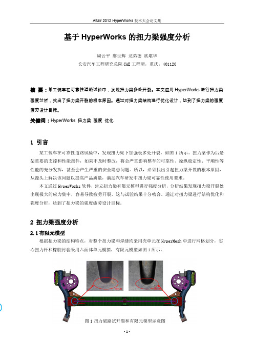
关键词:HyperWorks扭力梁强度优化1 引言某工装车在可靠性道路试验中,发现扭力梁下加强板多处开裂,如图1所示。
扭力梁作为后悬架重要的支撑和性能部件,如果不及时整改,将会严重影响整车的可靠性、操纵稳定性、平顺性等性能的充分发挥,甚至会产生严重的安全隐患问题。
所以,必须找出引起扭力梁开裂的根本原因,从源头上解决该问题以提高产品质量,满足汽车研发中扭力梁可靠性使用要求。
本文通过HyperWorks软件,建立扭力梁有限元模型进行强度分析,分析结果发现扭力梁开裂处出现极大的应力集中,容易导致疲劳开裂,这与试验结果十分吻合。
通过对扭力梁进行结构优化和强度分析,达到了扭力梁的强度疲劳设计目标。
2 扭力梁强度分析2.1有限元模型根据扭力梁的结构特点,对整个扭力梁和焊缝均采用壳单元在HyperMesh中进行网格划分,实心扭力杆和橡胶衬套采用六面体单元模拟,有限元模型如图1所示。
图1扭力梁路试开裂和有限元模型示意图2.2 材料属性为了提高计算结果的精度,计算中考虑了材料非线性和几何非线性,所以扭力梁使用的各种材料(如B510L 、Q235、DC04等等)不仅给出了它的弹性模量和泊松比,还给出了材料发生塑性变形后的应变和应力的关系曲线。
2.3 强度分析工况和设置悬架系统承受路面冲击载荷的大小与车辆行驶速度、路面状况和载重量等因素有关。
采用惯性释放方法,本文主要分析扭力梁在扭转极限工况下的强度,扭转极限工况下扭力梁各个接附点的载荷已通过多体动力学软件计算得到,如表1所示。
2.4 分析结果有限元模型经调试无误后提交计算,使用后处理软件HyperView 查看扭力梁整个结构的变形和应力分布,以及各零部件的应力大小等。
HYPERWORKS教程第14章_后处理
XIV 后处理本章部分材料来自于“Practical Finite Element Analysis”。
Kristian Holm, Hossein Shakourzadeh 和Matthias Goelke审阅并且添加了额外的内容。
请注意本章大多数内容是关于线性分析结果的后处理。
并非所有内容都适合碰撞和非线性分析。
14.1 如何判断和检查结果的准确性有限元分析是一门近似技术。
与试验数据相比,准确性可能达到25%、60%甚至90%。
下面的检查方法可以帮•肉眼检查——关键区域如果有应力不连续或者突变,那么应该对该区域进行细化。
•FEA和试验之间有10-15%的差距被认为是比较好的相关性。
•超过15%偏离的可能原因:错误的边界条件、材料属性、残余应力、局部效应如焊接,螺栓预紧、试验误差等。
14.2 如何判断和理解结果1) 第一重要原则首先要查看位移和变形的动画,然后才是其他的输出。
查看结果之前,闭上眼睛想象一下在给定载荷情况下物件应该如何变形。
软件计算所得结果应该能与其对上,部件不合理的位移和变形表明有些地方可能设置有误。
计算精度并不能保证有限元分析的正确性(比如部件在现实中的行为可能于软件预测的大相径庭)。
有必要与测试结果对比或得到有经验的CAE/测试工程师(他可能在类似的部件或产品上工作多年)的认可。
工程师需要有辨别能力,FE误差是来自于网格质量和数学模型的偏差,还是物理问题的模型假设。
为了能肉眼看到部件的变形,上图的位移结果被放大了。
由于位移值很小,真实的位移(1倍)可能无法观察到。
因此,多数的后处理软件提供了放大结果的功能(并非改变结果的真实大小)。
上图的位移云图中,位移被放大了100倍。
另外一个极其有用的可视化技术是动画。
这个功能对于理解静态分析的结果也是非常重要的。
模型的动画可以让用户深刻理解载荷(约束)对系统中结构的作用。
2) 检查反力、力矩、残余应变能和应变能比较施加载荷的合力或力矩、反力和反力矩、内功和外功、残余量可以帮助我们估计结果的数值精确性。
第三章 非线性分析

第三章非线性分析在工程结构实际中,常常会遇到许多不符合小变形假设的问题,例如板和壳等薄壁结构在一定载荷作用F,尽管应变很小,甚至未超过弹性极限,但是位移较大,材料微单元会有较大的刚体转动位移。
这时平衡条件应如实地建立在变形后的位形上,以考虑变形对平衡的影响。
同时应变表达式也应包括位移的二次项。
这样,结构的几何形变关系将是非线性的。
这种由于大位移和大转动引起的非线性问题称为几何非线性问题。
在涉及几何非线性问题的有限元方法中,可以采用两种不同的表达格式来建立有限元方程。
一种格式是所有静力学和运动学变量总是参考于初始位形的完全拉格朗日格式,即在整个分析过程中参考位形保持不变。
而另一种格式中,所有静力学和运动学的变量参考于每一载荷步增量或时间步长开始的位形,即在分析过程中参考位形是不断被更新的,这种格式就称为更新的拉格朗日格式。
下面将分别具体讨论大变形情况下应变和应力度量,几何非线性有限元方程的建立以及系数矩阵的形成。
在涉及几何非线性问题的有限元方法中,可以采用两种不同的表达格式来建立有限元方程。
一种格式是所有静力学和运动学变量总是参考于初始位形的完全拉格朗日格式,即在整个分析过程中参考位形保持不变。
而另一种格式中,所有静力学和运动学的变量参考于每一载荷步增量或时间步长开始的位形,即在分析过程中参考位形是不断被更新的,这种格式就称为更新的拉格朗日格式。
下面将分别具体讨论大变形情况下应变和应力度量,几何非线性有限元方程的建立以及系数矩阵的形成。
第三章非线性分析的数值计算方法3.1概述非线性问题一般包括三类:材料非线性、几何非线性和边界非线性;而在许多实际的结构中,常常是三种非线性问题的融合,因此其解析方法能够得到的解答是十分有限的。
对于非线性问题的求解,可以采用有限元分析的方法,因此非线性方程组的解法也就成为非线性问题有限元分析涉及的基本问题,也就是通常所说的非线性分析的数值计算方法I”。
常用的有Newton—Raphson法(简称N-R)和弧长法。
非线性分析
当F?Ku时的结构分析(非线性分析简介)1、引言1.1结构分析起源1.2有限元分析历史2、非线性的特征2.1材料非线性2.2几何非线性2.3边界条件非线性3、非线性有限元分析的概念3.1小应变3.2非线性应变-变形关系(几何方程)3.3非线性应力-应变关系(本构方程)3.4更新平衡方程3.5增量迭代求解方法4、大变形:更多关于几何非线性4.1总体拉格朗日方法4.2更新的拉格朗日方法4.3欧拉方法5、塑性:更多关于材料非线性5.1时间非相关行为5.2时间相关行为5.3屈服准则5.4硬化5.5蠕变(或称徐变)5.6粘弹性和粘塑性5.7橡胶和弹性体6、更多关于边界条件非线性6.1接触和摩擦7、非线性动力分析7.1动力问题求解方法7.2隐式解法7.3显式解法7.4两种方法的对比8、虚拟制造9、一些实用信息9.1非线性分析过程9.2网格细分和重划分10、应用实例10.1汽车业:汽车玻璃的非线性仿真辅助分析10.2航空业:Sikorsky Aircraft应用非线性求解方案解决设计瓶颈10.3土木工程:充气坝的非线性仿真分析,协助其运行一次成功10.4医疗器械:非线性有限元分析用于心血管器械的设计和安置1、引言结构和机械工程中的分析意味着基于工程原则的合适分析程序的应用,目的在于确定设计中结构的、热学的以及多种物理场的完整性。
对于简单结构,这些分析可以通过使用解析公式或其它方法解决。
更多时候,涉及到复杂部件或结构组装的分析就需要用到计算机仿真技术,这是虚拟产品开发(VPD)的一个组成部分。
用于此类分析的主要工程软件基于有限元方法,在过去50年里,有限元分析成功应用于航空、汽车、能源、制造、化工、电子、医学等所有主要工业领域。
事实上,有限元方法是现代计算机设计工程的主要突破之一。
1.1结构分析起源结构力学的起源可以追溯到伊萨克·牛顿和罗伯特·虎克等早期科学家。
对于一个刚度为K(单位N/m)的简易弹簧,自由端受力F(单位N)的作用,虎克得到了力荷载与引起的位移u之间简单的线性关系:f=Ku,此即虎克定律。
几何非线性分析非线性2几何非线性分析
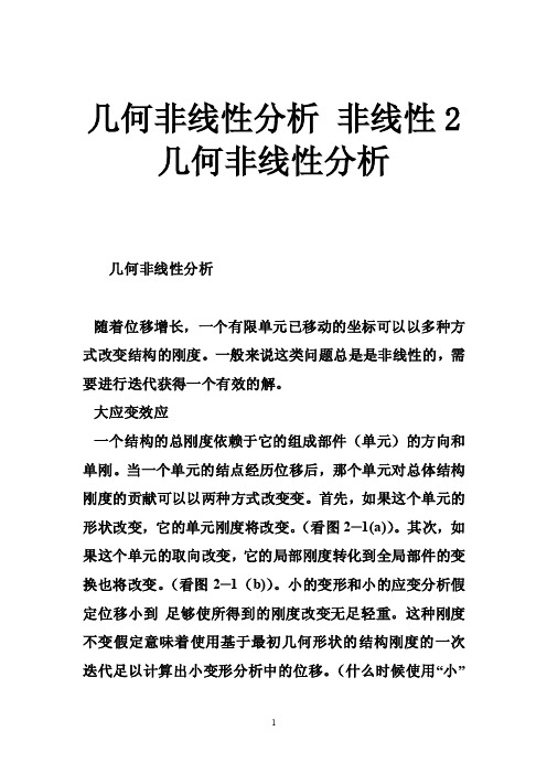
几何非线性分析非线性2几何非线性分析几何非线性分析随着位移增长,一个有限单元已移动的坐标可以以多种方式改变结构的刚度。
一般来说这类问题总是是非线性的,需要进行迭代获得一个有效的解。
大应变效应一个结构的总刚度依赖于它的组成部件(单元)的方向和单刚。
当一个单元的结点经历位移后,那个单元对总体结构刚度的贡献可以以两种方式改变变。
首先,如果这个单元的形状改变,它的单元刚度将改变。
(看图2─1(a))。
其次,如果这个单元的取向改变,它的局部刚度转化到全局部件的变换也将改变。
(看图2─1(b))。
小的变形和小的应变分析假定位移小到足够使所得到的刚度改变无足轻重。
这种刚度不变假定意味着使用基于最初几何形状的结构刚度的一次迭代足以计算出小变形分析中的位移。
(什么时候使用“小”变形和应变依赖于特定分析中要求的精度等级。
相反,大应变分析说明由单元的形状和取向改变导致的刚度改变。
因为刚度受位移影响,且反之亦然,所以在大应变分析中需要迭代求解来得到正确的位移。
通过发出NLGEOM,ON(GUI路径Main Menu>Solution>Analysis Options),来激活大应变效应。
这效应改变单元的形状和取向,且还随单元转动表面载荷。
(集中载荷和惯性载荷保持它们最初的方向。
)在大多数实体单元(包括所有的大应变和超弹性单元),以及部分的壳单元中大应变特性是可用的。
在ANSYS/Linear Plus程序中大应变效应是不可用的。
图1─11 大应变和大转动大应变处理对一个单元经历的总旋度或应变没有理论限制。
(某些ANSYS单元类型将受到总应变的实际限制──参看下面。
)然而,应限制应变增量以保持精度。
因此,总载荷应当被分成几个较小的步,这可以〔NSUBST,DELTIM,AUTOTS〕,通过GUI路径Main Menu>Solution>Time/Prequent)。
无论何时当系统是非保守系统,来自动实现如在模型中有塑性或摩擦,或者有多个大位移解存在,如具有突然转换现象,使用小的载荷增量具有双重重要性。
基于HyperWorks某变速器壳体强度分析与优化
基于HyperWorks某变速器壳体强度分析与优化赵志专;王同银【摘要】某款变速器在做静扭试验时,壳体出现长裂纹.借助HyperWorks仿真软件对壳体进行强度验证,提出改进方案.分析表明,后壳体油槽处有开裂倾向,与试验一致;通过更改油槽位置,优化壳体局部厚度,可降低壳体开裂风险.针对改进后的状态进行试验验证,结果表明优化方案可行.【期刊名称】《汽车零部件》【年(卷),期】2019(000)008【总页数】5页(P67-71)【关键词】静扭试验;变速器壳体;强度分析;结构优化【作者】赵志专;王同银【作者单位】南京越博动力系统股份有限公司,江苏南京210019;南京越博动力系统股份有限公司,江苏南京210019【正文语种】中文【中图分类】U463.2120 引言变速器可降速增扭,且可通过切换挡位,满足不同使用条件,保证了汽车的动力性和燃油经济性[1]。
静扭试验是一种测定变速器总成抵抗扭矩的试验,可反映变速器的强度。
汽车行业标准中规定,静扭强度后备系数需大于或等于规定值[2]。
HyperWorks[3]是功能强大的应用软件包,包含多个前处理、后处理工具,如HyperMesh、SimLab、HyperView,以及求解器OptiStruct,可完成不同类型的结构分析和优化。
公司某款变速器在试验扭矩3 570 N·m时,变速器内部齿坏,壳体开裂,如图1所示。
为保证试验完成时壳体无裂纹,现需对壳体结构进行优化。
迄今已有大量学者通过仿真或试验手段对变速器壳体强度进行研究。
吴仕斌等[4]应用ABAQUS软件对变速器总成铝壳体进行有限元分析,并进行试验验证。
黄德健等[5]考虑了变速器壳体承受内部齿轴力和外部冲击力的影响,应用RADIOSS计算铸铝壳体在一挡下的应力、变形的分布情况,并针对壳体薄弱处提出了优化方案。
宫唤春[6]在提高强度分析效率的同时,考虑了齿轮轴及轴承对变速器壳体强度的影响,为结构设计提供参考。
基于HyperWorks的汽车制动踏板静力分析流程自动化系统的设计
基于HyperWorks的汽车制动踏板静力分析流程自动化系统的设计肖洒;彭育辉【摘要】针对静力分析前处理过程中操作步骤繁琐,重复性工作量大等问题,本文结合企业实际CAE分析经验,设计出基于HyperWorks的汽车制动踏板静力分析流程自动化系统.该系统应用Tcl/Tk语言进行开发,实现了静力分析前处理流程的规范化,不仅可以引导CAE工程师完成流程的分析过程,而且大幅减少前处理操作时间,提高了工作效率.实践效果表明,该系统不仅提高了CAE分析工作效率,缩短了产品研发设计周期,同时也有.利于企业积累相关的CAE分析经验,对于企业有着相当明显的经济效益和积极意义.【期刊名称】《价值工程》【年(卷),期】2016(035)033【总页数】3页(P140-142)【关键词】HyperWorks;Tcl/Tk;制动踏板;静力分析;自动化系统【作者】肖洒;彭育辉【作者单位】福州大学机械工程及自动化学院,福州350002;福州大学机械工程及自动化学院,福州350002【正文语种】中文【中图分类】TP39;U266.2汽车制动踏板作为汽车操纵的五大件之一,由于使用频次非常高,其性能直接影响着汽车驾驶安全。
因此,相关企业在开发设计过程中广泛采用计算机辅助工程(Computer Aided Engineering,CAE)方法对制动踏板的强度刚度进行严格的强度刚度校核,以确保设计结构的可靠性和安全性。
虽然使用HyperWorks,ANASY等大型通用有限元分析软件进行产品结构的CAE分析可以有效缩短产品开发周期,减少企业研发成本[1],但使用此类有限元软件进行分析的操作较为复杂,基本依赖分析工程师的个人能力且不利于企业积累和传承相关使用经验。
因此根据产品设计的特点,对企业所使用的CAE软件进行具体的开发定制成为踏板设计CAE分析的一种必然需求。
而现实却是国内大多数企业对于CAE软件还只限于使用阶段,对CAE软件进行二次开发的研究并不是很多[2]。
hyperworks功能简介

Altair HyperWorks 功能简介一 .综合评价其为企业级CAE平台,集成设计与分析多种工具,拥有开放性体系和可编程工作平台,可提供顶尖的CAE建模、可视化分析、优化分析、以及健壮性分析、多体仿真、制造仿真、以及过程自动化。
二. 软件模块表1 HyperWorks软件模块分类1、OptiStruct 结构优化设计工具,提供拓扑、形貌、形状、尺寸等优化解决方案2、前后处理(1)HyperMesh高性能、开放式有限单元前后处理器,主要用于模型处理。
相对其它软件,具有更为强大的网格划分能力。
提供几乎所有主流商业CAD系统和CAE求解器接口。
CAD接口如ProE,CATIA,IGES,UG等。
CAE接口如ansys,optistruct,abaqus,nastran,dyna,ideas等(2)MotionView通用多体动力学仿真及工程数据前后处理器,拥有丰富的车身模型库并支持二次开发。
(3)HyperGraph仿真和实验结果的后处理绘图工具,拥有丰富的求解器和实验数据接口、数学函数库并支持后处理模块定制,实现数据处理自动化。
(4)HyperView完整的结果后处理工具,可处理有限元分析、多提系统仿真、视频和工程数据。
(5)HyperStudy为健壮性设计开发的参数化研究和多约束优化工具应用:实验设计(DOE)、随机仿真和优化技术3、求解器(1)OptiStruct/Analysis有限元分析求解器,具有快速而精确的特点应用:用于线性静态和频率响应分析的求解(2)MotionSolve多体动力学分析求解器应用:刚体和柔体耦合分析求解(3)Radioss应用:安全技术、生物仿真技术和车辆安全评价技术(4)HyperCrash应用:主要用于碰撞仿真4、制造工艺仿真(1)HyperForm钣金冲压成成形仿真工具,兼模具设计、管料弯曲成形和液压成形仿真模块(2)HyperXtrude 合金材料挤压成形仿真工具(3)Forging锻压方针(4)Molding注塑成型仿真(5)Friction Stir Welding模拟摩擦激光焊接三.软件应用1、拓扑优化:在给定的设计空间内寻求最佳的材料分布,载荷到约束的传力路径上材料得到保留。
结构非线性分析汇总
结构非线性分析理论1.结构设计方法结构设计方法从传统的容许应力设计法发展到了基于概率统计的极限状态设计法。
传统的容许应力设计法是基于线弹性理论,依照经验选取一定的安全系数,以构件危险截面某一点的计算应力不超过材料的容许应力为准则,目前在某些领域仍在使用。
安全系数,是一个单一的根据经验确定的数值,没有考虑不同结构之间的差异,不能保证不同结构具有同等的安全水平。
此外,容许应力设计法以弹性理论计算内力,对那些发展塑性变形能提高承载力的构件或结构(如受弯构件),比那些发展塑性变形不能提高承载力的构件或结构(如轴心受力构件)具有较大的安全储备。
概率极限状态设计法是采用数理统计方法按照一定概率确定荷载或材料的代表值,并给出结构的功能函数,用结构失效概率或可靠指标度量结构的可靠性。
《建筑结构可靠度设计统一标准》将极限状态分为两类:(1)承载能力极限状态,是指结构或结构构件达到最大承载能力或不适于继续承载的变形;(2)正常使用极限状态,是指结构或结构构件达到正常使用或耐久性能的某项规定限值。
结构按极限状态设计应符合下列要求:()0,21≥n X X X g (1.1)式((1.1)中g(X i )为结构功能函数,X i (i =1, 2……n)为基本变量,是指影响该结构功能的各种作用、材料性能、几何参数等。
目前我国结构设计规范基本都是采用以概率理论为基础的极限状态设计方法,用分项系数设计表达式进行计算。
美国的钢结构设计采用了两种设计方法:ASD(Allowable Stress Design)和LRFD(Load and Resistance Factor Design),即容许应力设计法和分项系数设计法,McCormac 指出LRFD 相比ASD ,并不一定节省材料,虽然在很多情况下可以取得这样的效果,而在不同荷载作用下能给结构提供等同的可靠性,对于活载和恒载,ASD 采用的安全系数是一样的,而LRFD 对恒载则采用了一个较小的荷载系数(恒载比活载能更准确的确定),也就是说如果恒载大于活载,LRFD 比ASD 节省材料。
03非线性分析要点

第三部分非线性分析第一章非线性有限元概述1.1非线性行为1、 非线性结构的基本特征是结构刚度随载荷的改变而变化。
如果绘制一个非线 性结构的载荷一位移曲线,则 力与位移的关系是非线性函数。
2、 引起结构非线性的原因:a 几何非线性:大应变,大位移,大旋转 (例如钓鱼竿的变形)b 材料非线性:塑性,超弹性,粘弹性,蠕变c 状态改变非线性:接触,单元死活3、 非线性行为一一分析方法特点A 不能使用叠加原理!B 结构响应与路径有关,也就是说加载的顺序可能是重要的。
C 结构响应与施加的载荷可能不成比例。
1.2非线性分析的应用1、 一些典型的非线性分析的应用包括: 非线性屈曲失稳分析金属成形研究碰撞与冲击分析制造过程分析(装配、部件接触等)材料非线性分析 (塑性材料、聚合物)2、 橡胶底密封:一个包含几何非线性(大应变与大变形),材料非线性(橡胶), 及状态非线性(接触)的例子。
2.1非线性方程组的解法1、求解一个结构的平衡问题通常等于求解结构的总位能的驻值 问题。
结构总位能n : 口 "3弋门心 2、 增量法:就是将荷载分成一系列的荷载增量,即 ANSYS 中的荷载步或荷载子 步。
A 要点:在每一个荷载增量求解完成后,继续进行下一个荷载增量之前, 刚度矩阵以反映结构刚度的变化。
B 增量法的优点:可以追踪结构变形历程,这对于材料或几何非线性(特别是 极限值屈曲分析)十分有用。
C 增量法的缺点:随着荷载步增量的增加而产生积累误差,导致荷载-位移曲 线飘移。
D 对飘移进行平衡修正,可以大大提高增量法的精度。
应用最广的就是在每一 级载荷增量上用Newton-Raphsor 或其变形的迭代法。
3、 迭代法:割线刚度法:收敛性差,因此很少应用切线刚度法Newto n-Ra phsor 迭代法:切向刚度法中 2.2 Newto n-Ra phsor 迭代法 1、 优点:对于一致的切向刚度矩阵有 二次收敛速度。
王 惠_HyperMesh在子午线轮胎三维非线性有限元分析的应用

HyperMesh在子午线轮胎三维非线性 有限元分析中的应用王惠 丁峻宏 韩轩上海超级计算中心HyperMesh 在子午线轮胎三维非线性有限元分析中的应用HyperMesh Application in Radial Tire 3D Non-Linear Finite Element Analysis王惠 丁峻宏 韩轩(上海超级计算中心 上海 201203)摘要:在HyperMesh中建立子午线轮胎的三维非线性有限元模型,用ABAQUS软件的非线性 分析技术对子午线轮胎进行了有限元分析。
考虑了轮胎的几何非线性,材料非线性,橡胶-帘线等复合材料的各向异性以及轮胎与地面的接触非线性,,给出了轮胎与地面接触过程中轮胎的变形情况,接触区域形状以及带束层应力分布情况。
对子午线轮胎的设计和改进具有一定的指导意义。
关键字:HyperMesh,子午线轮胎,非线性,有限元分析Abstract: A 3D non-linear finite element model of radial tire with contact with pavement is established using HyperMesh, radial tire’s finite element analysis is carried out using ABAQUS. With considerations of tire’s geometry non-linearity, material non-linearity, anisotropy of rubber-cord composite material and nonlinear contact of tire-pavement, deformation of the tire and tire belt layer’s effective stress are calculated and contact region contour are also described which gives helpful reference to radial tire structural design and improvement.Key word: HyperMesh, radial tire, non-linear, finite element analysis1引言轮胎是汽车和路面间传递力和力矩作用的唯一部件,具有优良的变形恢复能力和地面贴附能力,可以分散汽车对路面的压应力,降低汽车运动的能量损失,缓和行驶冲击,改善载荷条件等。
HyperWorks软件介绍与分析

Altair HyperWorks是一套杰出的企业级CAE仿真平台解决方案,它整合了一系列一流的工具,包括建模、分析、优化、可视化、流程自动化和数据管理等解决方案,在线性、非线性、结构优化、流固耦合、多体动力学、流体动力学、电磁场分析等领域有着广泛的应用。
仿真无处不在Altair HyperWorks 为工程师提供了完整的解决方案,涵盖从基于模型的系统设计、早期几何设计,到详细的多物理场仿真以及结构和多学科优化的整个产品设计周期。
HyperWorks提供的仿真驱动设计的解决方案,使工程师能更好地通过仿真理解复杂产品的物理本质,进而驱动更好的设计、满足客户的需求。
创成式设计的领导者20多年来,Altair一直是创成式设计领域的行业领导者。
HyperWorks可以优化结构、机构、复合材料和增材制造零件。
无论您的产品是如何生产的,HyperWorks都可以通过提出既高效又具有创新性的、可制造的设计来增强创造力。
统一的用户界面体验如今,设计师、工程师和CAE专家可以在一个直观的、一致的用户界面体验中工作。
HyperWorks平台提供了领先的解决方案,使得用户界面更加友好、前后处理软件界面风格更为统一。
对仿真专家和普通分析人员都适用的工具HyperWorks平台中众多的求解器和前后处理产品,方便设计工程师和普通分析人员能够快速轻松地通过优化来获得更多的产品设计。
仿真专家可以使用更多的高级功能,包括结构、机构、热、电磁和流体等多物理场仿真。
2019年6月10日Altair正式发布了Altair HyperWorks™ 2019。
新版本在单一开放式架构平台下为设计师及仿真工程师提供了更多的解决方案,可加快决策制定、缩短产品上市时间。
其亮点功能包括:✧复杂模型的快速仿真分析功能Altair SimSolid™可在几秒到几分钟内对未简化的原始CAD装配体进行结构分析,提高设计师及分析人员的工作效率。
SimSolid可分析复杂零件和大型装配体,而使用传统结构分析工具则可能会花费数小时或数天。
HyperWorks介绍

软件简介—S o f t W a r e?D e s c r i p t i o n A L T A I R?H y p e r W o r k s?7.0?S P1?HyperWorks?企业级的CAE软件,几乎所有财富500强制造企业都应用.为工程师量身定做的软件.强力推荐.?系列产品集成了开放性体系和可编程工作平台,可提供顶尖的CAE建模、可视化分析、优化分析、以及健壮性分析、多体仿真、制造仿真、以及过程自动化。
?HyperWorks的开放式平台可以直接运用顶尖的CAD、CAE求解技术,并内嵌与产品数据管理以及客户端软件包交互的界面。
?Altair?HyperWorks是一个创新、开放的企业级CAE平台,它集成设计与分析所需各种工具,具有无比的性能以及高度的开放性、灵活性和友好的用户界面。
HyperWorks包括以下模块:?Altair?HyperMesh?高性能、开放式有限单元前后处理器,让您在一个高度交互和可视化的环境下验证及分析多种设计情况。
?Altair?MotionView?通用多体系统动力学仿真及工程数据前后处理器,它在一个直观的用户界面中结合了交互式三维动画和强大无比的曲线图绘制功能。
?Altair?HyperGraph?强大的数据分析和图表绘制工具,具有多种流行的工程文件格式接口、强大的数据分析和图表绘制功能、以及先进的定制能力和高质量的报告生成器。
?Altair?HyperForm?集成HyperMesh强大的功能和金属成型单步求解器,是一个使用逆向逼近方法的金属板材成型仿真有限元软件。
?Altair?HyperOpt?使用各种分析软件进行参数研究和模型调整的非线性优化工具。
?Altair?OptiStruct?世界领先的基于有限元的优化工具,使用拓扑优化方法进行概念设计。
?Altair?OptiStruct/FEA?基本线性静态、特征值分析模块。
?创新、灵活、合理的许可证?无论是单机版还是网络版,HyperWorks?许可单位(HWUs)都是平行的,所以不管你运行多少个HyperWorks模块,只有需要HWUs最多的模块才占用HWUs数。
HyperWorks介绍

软件简介—SoftWare Description ALTAIR HyperWorks 7.0 SP1 HyperWorks 企业级的CAE软件,几乎所有财富500强制造企业都应用.为工程师量身定做的软件.强力推荐. 系列产品集成了开放性体系和可编程工作平台,可提供顶尖的CAE建模、可视化分析、优化分析、以及健壮性分析、多体仿真、制造仿真、以及过程自动化。
HyperWorks的开放式平台可以直接运用顶尖的CAD、CAE求解技术,并内嵌与产品数据管理以及客户端软件包交互的界面。
Altair HyperWorks是一个创新、开放的企业级CAE平台,它集成设计与分析所需各种工具,具有无比的性能以及高度的开放性、灵活性和友好的用户界面。
HyperWorks包括以下模块:Altair HyperMesh 高性能、开放式有限单元前后处理器,让您在一个高度交互和可视化的环境下验证及分析多种设计情况。
Altair MotionView 通用多体系统动力学仿真及工程数据前后处理器,它在一个直观的用户界面中结合了交互式三维动画和强大无比的曲线图绘制功能。
Altair HyperGraph 强大的数据分析和图表绘制工具,具有多种流行的工程文件格式接口、强大的数据分析和图表绘制功能、以及先进的定制能力和高质量的报告生成器。
Altair HyperForm 集成HyperMesh强大的功能和金属成型单步求解器,是一个使用逆向逼近方法的金属板材成型仿真有限元软件。
Altair HyperOpt 使用各种分析软件进行参数研究和模型调整的非线性优化工具。
Altair OptiStruct 世界领先的基于有限元的优化工具,使用拓扑优化方法进行概念设计。
Altair OptiStruct/FEA 基本线性静态、特征值分析模块。
创新、灵活、合理的许可证无论是单机版还是网络版,HyperWorks 许可单位(HWUs)都是平行的,所以不管你运行多少个HyperWorks 模块,只有需要HWUs最多的模块才占用HWUs数。
HyperWorks介绍和基础培训
常用基础操作介绍
1、焊缝的处理,通常采用的方法有: 1)通过rbe2进行连接;2)节点重合处理;3)采用梁单元
来模拟焊缝。
2、模型的运动关系的处理:通常是通过rbe2和梁单元共同来模 拟,通过释放自由度来实现运动关系。
3、力的加载区域的建立:一般是通过平移节点来得到需要的区 域大小
网格划分技巧介绍
所以必须使用工具使之清楚查看这两点,才能建立Spring。因为建 立Spring需要两个节点。 按O键(Operation)——Graphics——点击右侧的 Coincident picking
单元类型介绍
Gap单元
间隙伪单元(gap单元)能较好的反应“大面积接触区域性”的 特
点,提高求解的精度。
F 总 区 域 内 总 节 点 数 每 个 节 点 受 力 大 小
可以将该区域的所有节点设置为一个集合Sets,并且计算出 每个节点受力大小。以该值作为所加力的大小。但是,如果该区 域的网格重新划分了,那么就要重新加载。 (3)采用Pressure(压力)加载。
F总区域面积压力
力施加的是节点,而压力施加的是单元。这里同样可以将区域 的单元作为一个Set。同样,网格重新划分时加载也要更新。
1、巧用F7修改倒角处网格,另将节点拉直在一条直线上,再对 其他区域进行网格重划,得到较好的网格质量。 2、shift+F7进行网格的投影(平面、曲面、线) 3、shift+F4和reflect进行相同几何的网格复制 4、采用detach对局部区域的网格remesh,保持另一部分的网 格不受影响 5、采用rule、element offset、edit element等来修补缺失的单元
2、同一有限元模型可能存在多个载荷(即多个load collector ) 并且同一有限元模型的约束位置的约束自由度是不相同的。但是 在建立Load step时,只能选择一个载荷和一个约束。这些问题 将如何处理?
非线性分析

非线性分析线性分析在结构方面就是指应力应变曲线刚开始的弹性部分,也就是没有达到应力屈服点的结构分析。
非线性分析包括状态非线性,几何非线性,以及材料非线性。
状态非线性,比如就是钓鱼竿,几何比如就是物体的大变形,材料比如就是塑性材料属性。
两个区别其实很多,不过两个关键,一个就是材料定义的时候不同,[材料属性根据需要设置,静力学分析一般只要弹性模量和泊松比,如果考虑体载荷或动力学分析还需要定义密度(一般问题这样就可以了)]。
一个就是在求解设置选项的时候不同,因为非线性一般存在收敛困难的问题。
结构非线性中,最典型的分析是材料非线性[由于材料本身非线性的应力-应变关系导致的结构响应非线性叫材料非线性。
除了材料本身固有的应力-应变关系外,加载过程的不同,机构所处的环境的变化(如温度的变化)均可导致材料的应力应变的非线性。
]。
材料非线性包括弹塑性分析,蠕变分析,超弹性分析,弹塑性分析。
以金属为例,当应力低于比例极限,应力应变式线性的,当应力低于屈服强度,材料表现为弹性行为,就是说卸载后应变小时,应力超过屈服强度,应力-应变曲线表现为非线性,这个时候产生塑性行为,也就是卸载后,变形不能完全恢复,残留的部分变形就是塑性变形了。
对于超出屈服强度的部分,因为是塑性变形,所以要用塑性力学来求解,此时的分析手段是屈服准则和强化准则。
屈服准则就是当物体内一点出现塑性变形时,其所受应力必须满足的条件叫屈服准则,结构出浴一般应力状态时,是否达到屈服强度时需要通过屈服准则来检验的。
就是用理论上的一些判定原则,如果这些原则满足(充分条件满足),那么就够就达到了屈服强度。
屈服准则的值,叫等效应力,也可以说等效应力随着加载的增大到超过屈服应力是,就发生塑性变形,通用的屈服准则是Von Mises准则(这种准则除了土壤和塑性材料不能用,其它都可以用),脆性材料使用的准则是莫尔-库伦准则。
正如我们所知,很多结构响应与所受的外载荷并不成比例。
HyperWorks功能

XX集团澳汰尔工程软件(上海)有限公司二〇一三年四月目录1HyperWorks 软件的背景 (3)2Hyperworks 软件介绍 (3)2.1HyperMesh (3)2.2HyperView (7)2.3HyperGraph (8)2.4MotionView (9)2.5MotionSolve (11)2.6OptiStructy (12)1HyperWorks 软件的背景HYPERWORKS 软件由美国Altair Engineering, Inc开发。
公司成立于1985年,位于美国密歇根州底特律。
Altair Engineering, Inc是世界领先的工程设计技术的开发者之一,在CAE建模、可视化、结构优化和过程自动化等领域的软件产品始终站在技术的最前沿。
自成立以来,Altair 公司始终以为客户开发高效、实用的工程解决方案为己任,在工程技术创新方面不断获得大奖。
目前HYPERWORKS的全球用户超过3000家,在美国以外的13个国家设有分支机构。
作为一家CAE工程咨询公司,Altair公司在概念设计、结构优化、制造过程仿真和机械系统仿真等领域的经验在世界工业界得到了广泛的认可。
Altair公司的HyperWorks®产品已经被广泛应用于几乎所有的工业科技领域。
Altair公司分布在全球的专家精诚合作,利用独一无二的经验交流机制为客户创造解决方案,从而为客户极大地改进其工程产品的设计水平和质量、节约成本。
2001年Altair Engineering, Inc.来到中国,成立了全资子公司澳汰尔工程软件(上海)有限公司。
扎根中国,Altair将全力为中国客户提供更有效、更直接、更全面的工程服务。
2Hyperworks 软件介绍2.1 HyperMeshHyperMesh是一个针对主流有限元求解器的高性能前后处理软件,允许工程师在一个高度交互式和可视化的环境下分析产品的性能。
HyperMesh用户界面简单易学,并支持最广泛的几何CAD和CAE接口,增强协同能力和工作效率。
Hypermesh_Optistruct有限元非线性分析
Table of ContentsAbout This Book (7)1 Introduction to Nonlinearity (13)1.1 Sources of Nonlinearity (14)1.2 Features of Nonlinear Problems (15)1.3 When to Choose a Nonlinear Analysis? (17)1.4 Small vs Large Displacement Nonlinear Analysis (18)2 Solution Techniques (21)2.1 Incremental-Iterative Procedure (22)2.2 Automatic Increment Size Control (23)2.3 Convergence Criteria (24)2.4 Analysis Controls (24)2.5 Path Dependent Loading (31)2.6 Restarting a Nonlinear Analysis (33)2.7 Energy Output for Nonlinear Analysis (34)2.8 On the Fly Output of Displacement Results for Nonlinear Analysis (34)3 Material Nonlinearity (38)3.1 Elastic-Plastic Material (39)3.2 Hyperelastic Material (55)4 Geometric Nonlinearity (64)4.1 Large Deflection (64)4.2 Large Strain (66)4.3 Non-Uniqueness of the Solution: Snap-Through (68)4.4 Follower Forces (69)5 Contact Nonlinearity (77)5.1 Contact Discretization (77)5.2 Contact Types & Properties (90)5.3 Contact Utilities (99)5.4 Contact Setup – General Steps (117)5.5 Analysis Controls for Contacts (123)5.6 Contact Output (124)5.7 General Tips for Contact Setup (127)5.8 Tutorial : Nonlinear Analysis of an Interference Fit (127)5.9 Capstone Tutorial Part 1: Setting Up Frictional Contact in a Bolted Pipe (140)6 Bolt Pretension (145)6.1 Pretensioning Process (145)6.2 Bolt Pretension in OptiStruct (146)6.3 Capstone Tutorial Part 2: Creating Pretensioned 3D Bolts in the Bolted (151)7 Analyzing Gaskets (156)7.1 Loading/Unloading Data Setup (156)7.2 Gasket Material & Property Cards (158)7.3 Gasket Elements Setup (160)7.4 Capstone Tutorial Part 3: Creating Gaskets for the Bolted Pipe Flange (161)8 Nonlinear Direct Transient Analysis (167)8.1 Solution Method (168)8.2 Nonlinear Transient Analysis Setup (169)8.3 Tutorial: Nonlinear Transient Analysis of a Plate with a Hole (171)9 Tips and Tricks (178)9.1 Essential Steps To Start With Nonlinear FEA (178)9.2 Debugging (179)9.3 Useful Tutorials and Industry Examples (181)10 Appendix (185)About This BookThis study guide aims to provide a fundamental to advanced approach into the exciting and challenging world of NonLinear Analysis. The focus will be on aspects of NonLinear Dynamic Analysis. As with our other eBooks we have deliberately kept the theoretical aspects as short as possible.The tool of choice used in this book is OptiStruct. Altair ® OptiStruct® is an industry proven, modern structural analysis solver for linear and nonlinear structural problems under static and dynamic loadings. OptiStruct is used by thousands of companies worldwide to analyze and optimize structures for their strength, durability and NVH (noise, vibration and harshness) characteristics.In this eBook, we will describe in some detail:•Nonlinear Materials•Nonlinear Geometry•Contacts•Bolt Pretension•Gasket Analysis•Nonlinear Direct Transient AnalysisPlease note that a commercially released software is a living “thing” and so at every release (major or point release) new methods, new functions are added along with improvement to existing methods. This document is written using HyperWorks Solvers 2018.0. Any feedback helping to improve the quality of this book would be very much appreciated.Thank you very much.Dr. Matthias GoelkeOn behalf of the Altair University TeamModel FilesThe models (geometry) referenced in this book can be downloaded using the link provided in the exercises, respectively. These model files are based on HyperWorks OptiStruct 2017. You can download the HyperWorks 2017 model files from here ... These models are compatible with the latest version.SoftwareObviously, to practice you need to have access to HyperWorks. As a student, you are eligible to download and install the free Student Edition:https:///free-hyperworks-2017-student-edition Note: From the different software packages listed in the download area, you just need to download and install HyperWorks.SupportIn case you encounter issues (during installationbut also how to utilize Altair HyperWorks) postyour question in the moderated Support Forumhttps://It’s an active forum with several thousands ofposts – moderated by Altair experts!Free eBooksIn case you are interested in more details about the “things” happening in the background we recommend our free eBookshttps:///free-ebooks-2Learning & Certification ProgramMany different eLearning courses are available for free in theLearning & Certification Program.For instance, you may find this eLearning course helpful:Learn Mechanics of Solids Fundamentalshttps:///course/view.php?id=66T his course is to introduce the subject of mechanics of solids with a focus on theory. Of course, there is also an eLearning course about HyperWorks availableFor OptiStruct Nonlinear Analysis, the prerequisite (or recommended) course is Structural Analysis:Learn Structural Analysis with OptiStructhttps:///course/view.php?id=71Acknowledgement“If everyone is moving forward together, then success takes care of itself” Henry Ford (1863 -1947)A very special Thank You goes to all the many colleagues who contributed in different ways:Gabriel Stankiewicz for writing the first draft of the book. Sanjay Nainani for the review of manuscript for the first edition. Rahul Rajan for editing, reviewing & updating the new features in the second edition of this book. Prakash Pagadala for helpful discussions and explanations.Rahul Ponginan for overall review of the book. Premanand Suryavanshi, Priyanka Nagraj, Pranav Harikrishnan and Nimisha Srivastava for the valuable support. For sure, your feedback and suggestions had a significant impact on the “shape” and content of this book.Sean Putman and Elizabeth White for all the support, especially with respect to the video recordings used in here.Junji Saiki, Warren Dias, Ujwal Patnaik and Girish Mudigonda from OptiStruct team.Mike Heskitt, Nelson Dias, Pavan Kumar, Rajneesh Shinde & Dev Anand for all the support.The entire Altair HyperWorks Documentation Team for putting together 1000’s of pages of documentation.Lastly, the entire Altair OptiStruct team deserves huge credit for their passion & dedication! It is so exciting to see how OptiStruct has evolved throughout the last couple of years.DisclaimerEvery effort has been made to keep the book free from technical as well as other mistakes. However, publishers and authors will not be responsible for loss, damage in any form and consequences arising directly or indirectly from the use of this book. © 2018 Altair Engineering, Inc. All rights reserved. No part of this publication may be reproduced, transmitted, transcribed, or translated to another language without the written permission of Altair Engineering, Inc. To obtain this permission, write to the attention Altair Engineering legal department at:1820B ig Beaver, Troy, Michigan, USA, or call +1-248-614-2400.1 Introduction to NonlinearityIn this book, we discuss the practical aspects of Nonlinear Finite Element Analysis. But how do we know that our problem is nonlinear? The best way is to look at the load-displacement response of one or more characteristic load introduction points. As discussed in one of our earlier books on Type of Analyses, when the structural response (deformation, stress and strain) is linearly proportional to the magnitude of the load (force, pressure, moment, torque, temperature etc.), then the analysis of such a structure is known as linear analysis. When the load to response relationship is not linearly proportional, then the analysis falls under nonlinear analysis (see figure below). For example, when a compact structure made of stiff metal is subjected to a load relatively lower in magnitude as compared to the strength of the material, the deformation in the structure will be linearly proportional to the load and the structure is known to have been subjected to linear static deformation. But most of the time either the material behavior is not linear in the operating conditions or the geometry of the structure itself keeps it from responding linearly. Due to the cost or weight advantage of nonmetals (polymers, woods, composites etc.) over metals, nonmetals are replacing metals for a variety of applications. These applications have nonlinear load to response characteristics, even under mild loading conditions. Also, the structures are optimized to make most of its strength, pushing the load level so close to the strength of the material, that it starts behaving nonlinearly. In order to accurately predict the strength of the structures in these circumstances, it is necessary to perform a nonlinear analysis.As discussed in the earlier chapter, the stiffness matrix relating to the load and response is assumed to be constant for static analysis; however, all the real-world structures behave nonlinearly. The stiffness matrix consists of geometric parameters such as length, cross sectional area and moment of inertia, etc. and material properties such as elastic modulus, rigidity modulus etc. The static analysis assumes that these parameters do not change when the structure is loaded. On the other hand, nonlinear static analysis considers the changes in these parameters as the load isapplied to the structure. These changes are accommodated in the analysis by rebuilding the stiffness matrix with respect to the deformed structure (i.e. altered properties) after each incremental load application. Although, the world is nonlinear, it should be mentioned that in many cases the assumption of linearity is valid and in that way a linear analysis can be done instead. Also, from a computation point of view, it is a much less expensive approach.1.1 Sources of NonlinearityNonlinear analysis should be introduced when the linear solution is not valid anymore, this can be caused by any one of the three main sources of nonlinearity:•Material nonlinearityMaterial nonlinearity is caused by plasticity i.e. material stiffness changes as the strain increases.Material nonlinearity involves the nonlinear behavior of a material based on current deformation, deformation history, rate of deformation, temperature, pressure, and so on.•Geometric nonlinearityIn analyses involving geometric nonlinearity, changes in geometry as the structure deforms are considered in formulating the constitutive and equilibrium equations. Many engineering applications require the use of large deformation analysis based on geometric nonlinearity. Applications such as metal forming, tire analysis, and medicaldevice analysis. Small deformation analysis based on geometric nonlinearity is required for some applications, like analysis involving cables, arches and shells. Such applications involve small deformation, except finite displacement or rotation.•Boundary and Contact NonlinearityPresence of contact definition between two bodies imposes an additional condition that they do not penetrate each other. During relative displacement, the bodies may come in contact which in fact happens to be an additional displacement constraint for them, this causes a nonlinearity called boundary nonlinearity. During large displacements, we may also require that pressure is normal to the moving surface, so that it moves with respect to the global coordinate system. This is also classified as boundary nonlinearity.Images after K.J. Bathe, Finite Elemente Methoden1.2 Features of Nonlinear ProblemsNonlinear problems need consideration of several features that are especially characteristic:•Non-uniqueness: For an applied load P there may be no solution, one solution, or many displacement solutions uA great example is snap through behavior of a shallow curved plate. Notice that for certain P values, there can even be 3 different solutions of displacement u, such an example presents a history-dependent behavior.•Non-scalability: If an applied load P causes displacement u, then an applied load x times P may not cause displacement x time u,•No superposition: If an applied load P causes displacement u and load F causes displacement d, then P+F may not cause displacement u+dOverview1.3 When to Choose a Nonlinear Analysis?Choice of a proper analysis type is sometimes not done correctly due to insufficient knowledge about the problem being examined. Often a simpler solver solution is chosen and complexity of the situation is neglected, such as choosing linear analysis when the problem needs plasticity considerations. Below a chart is presented that shows how one should investigate the type of analysis that is applicable for a structural problem. Five types of analyses are presented that in fact are somehow similar - it is sometimes parameters, like velocity, strains and forces that are critical to a proper choice of solution from the below presented analyses.Difference between Nonlinear Quasi-Static Analysis and Nonlinear Transient Analysis:The Nonlinear Quasi-Static Analysis differs from a transient analysis due to its assumption that time and hence inertial forces and momentums are negligible. One may even wonder why we compare nonlinear analysis to time-dependent solutions. As explained before, the solution for nonlinear analysis also considershistory-Is inertial behavior still relevant?NOYESDoes our problemcontain nonlinearity?NOYESLinear Static Analysis Nonlinear Quasi-Static Analysis Does our problemcontain nonlinearity?NOYESLinear TransientAnalysis RADIOSS Explicit Dynamic Analysisdependent behavior. Therefore, both solutions consider an incremental approach, but nonlinear quasi-static analysis increments are loading-based instead of time-based. This topic will be discussed further in the next chapter.1.4 Small vs Large Displacement Nonlinear AnalysisOptiStruct can perform two types of Quasi-Static analyses, depending on the types of nonlinearities available in the model. Below is a table that describes most relevant differences for small and large displacement analyses.Type Small Displacement NonlinearAnalysis Large Displacement Nonlinear AnalysisOverview Finds application mainly whenthe nonlinearity is limited tocontact and small strains. Thistype will not accurately solvefor larger displacements,significant geometry changeand when following forces arerequired. Accurately solves problems containing large deformations, rotations, displacements. Applicable to all types of nonlinearity.Remarks Active by default (LGDISP,0) Must be activated by changingthe LGDISP control card to 1.Needs to be used together withhash assembly option(PARAM,HASHASSM,YES). Strain range 0 < ε < 5% (recommended) ε > 5% (recommended)Material nonlinearity Supported only for MATS1elastic-plastic material.Supported for both MATS1elastic-plastic and MATHEhyperelastic material ofpolynomial form.Type Small Displacement NonlinearAnalysis Large Displacement Nonlinear AnalysisContact nonlinearity Supported(However, no update ofgap/contact element locationsor orientation due to geometry change)SupportedFollowerloadsNot supported SupportedSupported elements All generally used elementtypes are supportedSolid elements, Shell (first orderonly) elements,CBUSH, RROD,CELASi, RBAR, RBE2, and RBE3.Composites using PCOMP,PCOMPG, and PCOMPP entriesare supported2 Solution TechniquesGenerally, there are two main techniques to solve nonlinear problems:•Explicit, which is used to solve highly nonlinear dynamic problems - implemented in RADIOSS,•Implicit, which assumes that the simulated process runs infinitely slowly (Nonlinear Quasi-Static Analysis) or in a longer period of time (Nonlinear Direct Transient Analysis).Key differences between these two methods are presented in the table:Method Implicit ExplicitSolver OptiStruct, RADIOSS RADIOSSEquilibrium equations Static equilibrium (Quasi-Static)Dynamic equilibrium (Transient)Dynamic equilibriumStability Unconditionally stable (stabilityof the system does not dependon increment size) Conditionally stable (stability of the system depends on an increment time step, which in turn depends on smallest element size and material properties)Procedure Incremental and iterative (eachload increment consists ofseveral iterations untilconvergence is reached)IncrementalTime step size Larger time steps are used, sinceafter each increment Newton-Raphson iterations areperformed until the solution isconvergent enough.Much smaller time steps -small enough to assume thesolution is accurate, noiterations are performed.Application Static nonlinear eventsRelatively slow speed events(Transient) or allowingassumption of fully static (Quasi-Static) features. Highly dynamic events, occurring in relatively short period of timeTo solve Nonlinear Quasi-Static problems, OptiStruct applies implicit method.2.1 Incremental-Iterative ProcedureAlthough in Nonlinear Quasi-Static Analysis time is not considered and we omit any dynamic effects, the solution is always history-dependent (non-uniqueness of the solution), hence, we need to apply loading in small increments.Since the increments are much larger than in the explicit method accuracy is not achieved and therefore several iterations need to be performed to achieve certain, user-defined convergence criteria. Such iterations may sometimes be time consuming, but on the other hand the increment size can be even a few orders bigger than for explicit. In the figure below, an increment calculation procedure is shown.Consider a nonlinear problem:Where, u is the displacement vector, f is the global load vector, and L(u) is the nonlinear response of the system (nodal reactions). Note that for a linear problem, L(u) would simply be Ku (as described in Linear Static Analysis). Application of Newton's method to this equation leads to an iterative solution procedure:Where,In the above formulas, Kn represents a "slope" matrix, defined as a tangent to the L(u) curve at a point un, and Rn is the nonlinear residual. Repeating this procedure iteratively, under certain convergence conditions, leads to systematic reduction of residual Rn and hence, convergence.Note: Specifically, only for small displacement nonlinear analysis, that the above scheme is somewhat modified to an equivalent format wherein, instead of calculating Δun, the new solution un+1 is directly obtained:This form is readily produced by adding Kn un to both sides of Newton's equation, and has certain advantages in practical implementations.2.2 Automatic Increment Size ControlChoosing a suitable time increment is very important. In OptiStruct, an automatic time increment control is available. It should be suitable for a wide range of nonlinear problems and, in general, is a very reliable approach. In future OptiStruct versions, additional user control options to set up automatic time increments may be provided.The automatic time increment control functionality measures the difficulty of convergence at the current increment. If the calculated number of iterations is equal to optimal number of iterations for convergence, OptiStruct will proceed with the same increment size. If a lesser number of iterations is required to achieve convergence, the increment size will be increased for next increment. Similarly, if it is determined that too many iterations are required, the current increment will be attempted again with a smaller increment size.2.3 Convergence CriteriaAs mentioned before, the iteration process for a single increment is repeated until certain convergence criteria are met, by default there are three convergence criteria activated, so that means all of them must be met simultaneously. They are: Relative error in displacement EU (printed as EUI in OUT file):E U=q1−q‖A∙∆u‖‖A∙u‖where ‖A∙u‖=�|A i u i|i and q=‖∆u n‖‖∆u n−1‖Relative error in terms of load EP (printed as EPI in OUT file):E P=‖R∙u‖‖P∙u‖Relative error in work EW (printed as EWI in OUT file):E W=‖R∙∆u‖‖P∙u‖For more information regarding convergence criteria, please refer to Help documentation.2.4 Analysis ControlsThe incremental-iterative procedure due to its complexity needs to be controlled by several parameters. Hence, user can specify them through load collectors with proper card images, which are later referenced by NLQS load step. The basic card image is NLPARM, which controls the main parameters. Besides that, user can additionallyspecify NLADAPT to define more detailed time step and convergence controls. NLOUT allows one to request for additional results to an h3d file.2.4.1 Main Parameters - NLPARMMain parameters that control the Nonlinear Quasi-Static Analysis load step are defined within NLPARM card, which is activated as a Load Collector. Some of the most useful parameters, referenced in this card, are shown below (parameters which are important to understand during the first steps of NL analysis are presented in bold letters): Where:(1) (2) (3)(4) (5) (6) (7) (8) (9) (10) NLPARM IDNINC DT KSTEP MAXITER CONVEPSU EPSP EPSW MAXLS LSTOLTTERM IDIdentification number (must be unique) NINCNumber of implicit load sub-increments. DTInitial load increment MAXITERLimit on number of implicit iterations for each load increment. CONV Flags to select implicit convergence criteria.EPSU, EPSP, EPSWError tolerance for displacement (U), load (P), and work (W) criteria. MAXLSMaximum number of line searches allowed for each iteration. LSTOLLine search tolerance. TTERMTermination time.•Number of load increments (NINC or alternatively DT + TTERM)When NINC is not specified, there will be only one increment (full loading at once) applied during simulation, this causes high risk of divergence and error. With significantly nonlinear problems, it is recommended to use even NINC = 1000 (0.001 load increments), mildly nonlinear problems can be solved with NINC = 10.NINC number defines only initial increment size. Since automatic control is used for increment size – it may change over the analysis progress.It is recommended that the analysis usually should start with smaller increments than the targeted one.Alternatively, analysis increment size can be defined by use of DT (initial increment size) and TTERM (termination time) entries. These options are used for user-defined load curve, i.e. instead of defining only the end value of the load, one can also specify the load path TLOAD1 bulk data entry via DLOAD in the subcase information entry. When both DT and NINC are specified, DT will be used.2.4.2 Additional Time Step and Convergence Controls – NLADAPT Sometimes additional parameters may help achieve convergence for e.g. terminate diverging simulation earlier, saving time spent waiting until the simulation ends. Through this card user can also specify whether increment size should be adaptive (automatic control, as described before) or fixed (constant increment size).ID Unique identification numberNCUTS Number of cutbacks allowed to reduce the time increment.DTMAX Maximum time increment allowed.DTMIN Minimum time increment allowed.NOPCL Number of grids allowed to have open-close contact status change.NSTSL Number of grids allowed to have stick-slip contact status change when the current time step converged.EXTRA Determines whether to use linear extrapolation for load increments.DIRECT Sets adaptive or fixed time increment scheme.• NCUTS – available only for LGDISP . This parameter controls how many timessolver can reduce the load increment (within one increment) after divergence occurs. By default, it is 5, which is reasonable for most of the cases.• DTMAX and DTMIN – available only for LGDISP . There are cases, when we willwant to specify the maximum time increment allowed, for instance, to obtain accurate information about intermediate results, view smoother animation during postprocessing. DTMIN can also be specified to omit large analysis time for instance.• DIRECT – as mentioned earlier, user can specify a fixed increment (DIRECT,YES )for the whole analysis (NLPARM,NINC + NLADAPT,DIRECT,YES ), when certain intermediate results are required. However, this often leads to divergence, as a larger nonlinearity is present. In that case, either NINC should be lowered or DIRECT set to default NO .2.4.3 Request for Intermediate Results with NLOUT • NINT – user can request for results after each increment, so that the loadingprocess can be displayed later in HyperView.• SVNONCNV – also, a nonconvergent result from the last increment can berequested, it sometimes may help debugging by viewing what happened in the IDUnique identification number NINTNumber of intervals specified to output intermediate results. SVNONCNVFlag to output the non-convergent solution, if nonlinear iterations does not converge.model during last converged increments. Activate SVNONCNV,YES to write h3d file containing non-convergent solution2.4.4 Helpful Analysis Control Tool – EXPERTNLNonlinear expert system allows users flexibility in solving nonlinear solutions •PARAM, EXPERTNL,AUTO (default)/YES/CNTSTB/NO•The expert system monitors the convergence of nonlinear processes and tries to improve the convergence for poorly converging cases•“YES” activates an ‘expert system’ that aids in the convergence. Possible actions like performing additional iterations, under-relaxation, automatic adjustment of the load increment, backing off to the last converged solution and retrying. May lead to a large number of nonlinear iterations.•“AUTO” activates a ‘light’ version of the expert system which facilitates converging nonlinear process in reasonably close to minimum number of iterations.•“CNTSTB” introduces temporary stabilization on contact interfaces to improve nonlinear convergence (discussed further in contact topic).Adaptive load increment technique with the expert system (PARAM, EXPERTNL) is currently not supported with large displacement nonlinear analysis. However, the stabilization with PARAM,EXPERTNL,CNTSTB is supported for large displacement analysis.2.4.5 Loadsteps SequenceIt may so happen that a simulation run must involve a sequence of different loading cases (loadcase) one after another. That means, a result from some specific loadcase needs to be taken as the initial model condition for the next loadcase. Such a configuration is used when a loading-unloading cycle is evaluated for e.g. some metal forming processes consist of a few steps in a sequence. Below is an example of a loading-unloading cycle of a chair subjected to plastic deformation:Here one thing should be mentioned additionally. Despite being unloaded in the final state, the chair remains largely deformed. It is actually another very good example that proves the history-dependent character of NL analysis. Initial and final states are not subjected to any load, but due to load path that was applied to the model in the meantime, chair model ended up with pure plastic deformation. Loaded state deformation is a sum of elastic and plastic strains, here one can see that elastic strain was just a minor part (small difference between loaded and unloaded state). Continuation of multiple subcases is activated through CNTNLSUB card, this can be done in two ways:TNLSUB activation in SUBCASE OPTIONS, where following options areavailable•CNTNLSUB = YES:This nonlinear subcase continues the solution from the nonlinear subcase preceding. “Preceding” refers to the sequence in the input deck and NOT thenumbering of the subcases•CNTNLSUB = NO:This nonlinear subcase executes a new solution sequence starting from theinitial, stress-free state of the model.•CNTNLSUB = SID:。
hyperworks非线性分析理论详解
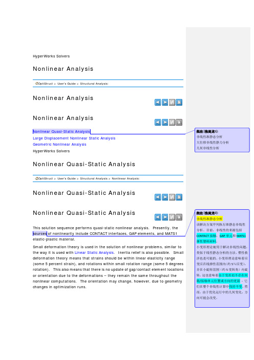
批注 [张剑龙2]: 非线性准静态分析 该解决方案序列执行准静态非线性 分析。目前,非线性的来源包括 CONTACT 接触,GAP 单元和 MATS1 弹性塑料材料。 小变形理论被用于解决非线性问题, 类似于线性静态分析的方法。惯性救 济也是可能的。小变形理论意味着应 变应在线弹性范围内(约 5%应变), 并在小旋转范围(约 5 度转角)内旋 转。这也意味着由于变形而不存在间 隙/接触单元位置或方向的更新 - 它 们在整个非线性计算中保持不变。然 而,由于优化运行中的几何变化,方 向可能会改变。
This solution sequence performs quasi-static nonlinear analysis. Presently, the sources of nonlinearity include CONTACT interfaces, GAP elements, and MATS1 elastic-plastic material.
OptiStruct > User's Guide > Structural Analysis > Nonlinear Analysis:
Nonlinear Quasi-Static Analysis
批注 [张剑龙1]: 非线性准静态分析 大位移非线性静力分析 几何非线性分析
Nonlinear Quasi-Static Analysis
This procedure, known as incremental loading, helps to keep the consecutive iterations closer to the true load path, thereby improving the chances of obtaining a final, converged solution (though usually at the expense of an increased total number of iterations).
- 1、下载文档前请自行甄别文档内容的完整性,平台不提供额外的编辑、内容补充、找答案等附加服务。
- 2、"仅部分预览"的文档,不可在线预览部分如存在完整性等问题,可反馈申请退款(可完整预览的文档不适用该条件!)。
- 3、如文档侵犯您的权益,请联系客服反馈,我们会尽快为您处理(人工客服工作时间:9:00-18:30)。
Incremental Loading
For a large class of problems satisfying certain stability and smoothness conditions, the Newton's iterative method is proven to converge, provided that the initial guess is sufficiently close to the true force-displacement path L(u). Hence, to improve convergence for strongly nonlinear problems, the total loading P is often applied in smaller increments, as shown in the figure below. At each of the intermediate loads, P1, P2, etc., the standard Newton iterations are performed.
Where,
In the above formulas, Kn represents a "slope" matrix, defined as a tangent to the L(u) curve at a point un , and Rn is the nonlinear residual. Repeating this procedure iteratively, under certain convergence conditions, leads to systematic reduction of residual Rn and hence, convergence.
Nonlinear Solution Method
The basic Newton method is used for the solution of nonlinear problems. The principle of this method is illustrated for a one-dimensional problem in the figure below and can be formulated as follows:
Small deformation theory is used in the solution of nonlinear problems, similar to the way it is used with Linear Static Analysis. Inertia relief is also possible. Small deformation theory means that strains should be within linear elasticity range (some 5 percent strain), and rotations within small rotation range (some 5 degrees rotation). This also means that there is no update of gap/contact element locations or orientation due to the deformations – they remain the same throughout the nonlinear computations. The orientation may change, however, due to geometry changes in optimization runs.
批注 [张剑龙5]: 非线性收敛准则 为了评估非线性过程是否收敛,可以 使用多个收敛准则。可以在 NLPARM 批量数据卡上选择这些标准和相应 的公差。评估非线性收敛的基本原理 是将解决方案的误差测量与预定的 公差水平进行比较。当误差低于规定 的公差时,该问题被认为是收敛的。 在多个同时收敛标准的情况下,需要 满足要收敛的解的所有标准。
Nonlinear Quasi-Static Analysis
This solution sequence performs quasi-static nonlinear analysis. Presently, the sources of nonlinearity include CONTACT interfaces, GAP elements, and MATS1 elastic-plastic material.
这种形式很容易通过在牛顿方程的 两边添加 Kn un 而产生,并且在实际 实现中具有一定的优点。
Note that the above scheme is somewhat modified to an equivalent format wherein,
instead of calculating
其中,u 是位移矢量,P 是全局负载 矢量,L(u)是系统的非线性响应(节 点反应)。 注意,对于线性问题,L (u)将简单地是 Ku(如线性静态分 析部分所述)。 牛顿方法在这个方程 中的应用导致迭代解法:
其中,
在上述公式中,Kn 表示“斜率”矩 阵,定义为在点 un 处的 L(u)曲线 的切线,Rn 是非线性残差。 在一定 的收敛条件下迭代地重复这个过程, 导致残差 Rn 的系统减少,从而导致 收敛。 注意,上述方案被稍微修改为等价格 式,其中,代替计算,直接获得新解 un + 1:
The relative error in displacements (printed in the convergence summary as EUI) is calculated as:
Here, A is a normalizing vector consisting of square roots of diagonal elements of
Nonlinear Convergence Criteria
In order to assess whether the nonlinear process has converged, a number of convergence criteria are available. These criteria and respective tolerances can be
This procedure, known as incremental loading, helps to keep the consecutive iterations closer to the true load path, thereby improving the chances of obtaining a final, converged solution (though usually at the expense of an increased total number of iterations).
HyperWorks Solvers
Nonlinear Analysis
OptiStruct > User's Guide > Structural Analysis:
Nonlinear Analysis
Nonlinear Analysis
Nonlinear Quasi-Static Analysis Large Displacement Nonlinear Static Analysis Geometric Nonlinear Analysis HyperWorks Solvers
stiffness matrix
and the vector norm II. II is calculated as:
批注 [张剑龙6]: 位移的相对误差(作为 EUI 汇总在汇 总表中表示)计算为:
Nonlinear Quasi-Static Analysis
OptiStruct > User's Guide > Structural Analysis > Nonlinear Analysis:
Nonlinear Quasi-Static Analysis
批注 [张剑龙1]: 非线性准静态分析 大位移非线性静力分析 几何非线性分析
批注 [张剑龙3]: 非线性解法 基本的牛顿法用于解决非线性问题。 该方法的原理如下图所示,用于一维 问题,可以表达如下:
考虑一个非线性问题:
Consider a nonlinear problem:
Where, u is the displacement vector, P is the global load vector, and L(u) is the nonlinear response of the system (nodal reactions). Note that for a linear problem, L(u) would simply be Ku (as described in the Linear Static Analysis section). Application of Newton's method to this equation leads to an iterative solution procedure:
, the new solution un+1 is directly obtained:
This form is readily produced by adding Kn un to both sides of Newton's equation, and has certain advantages in practical implementations.
批注 [张剑龙2]: 非线性准静态分析 该解决方案序列执行准静态非线性 分析。目前,非线性的来源包括 CONTACT 接触,GAP 单元和 MATS1 弹性塑料材料。 小变形理论被用于解决非线性问题, 类似于线性静态分析的方法。惯性救 济也是可能的。小变形理论意味着应 变应在线弹性范围内(约 5%应变), 并在小旋转范围(约 5 度转角)内旋 转。这也意味着由于变形而不存在间 隙/接触单元位置或方向的更新 - 它 们在整个非线性计算中保持不变。然 而,由于优化运行中的几何变化,方 向可能会改变。