直方图统计及均衡化matlab代码
直方图均衡化实例
实验一直方图的均衡化一.实验目的1.熟练使用opencv编写程序。
2.熟悉并运用直方图均衡话的方法处理图像。
二.实验原理及代码#include "cv.h"#include "highgui.h"#include "stdio.h"#include "stdlib.h"#include "math.h"#define LEVEL 256int main( int argc, char** argv ){IplImage* pImgSource,*pImgDestination; //声明IplImage指针int height,width,stepSource,stepDestination,channels,grayLevel[LEVEL], pixelsC[LEVEL];uchar *dataSource,*dataDestination;int i,j,k,p;//载入图像pImgSource = cvLoadImage("couple.bmp");if( !pImgSource ){printf("Image was not loaded.\n");return -1;}//获取图像信息height = pImgSource->height;width = pImgSource->width;stepSource = pImgSource->widthStep;channels = pImgSource->nChannels;dataSource = (uchar *)pImgSource->imageData;printf("Processing a %d*%d with %d channels\n",height,width,channels);//获得NO. of pixelsfor(i = 0; i < LEVEL; i++)grayLevel[i] = 0; // 初始化灰度级数组for(i = 0; i < height; i++)for(j = 0; j < width; j++)for(k = 0; k < channels; k++) {p = dataSource[i*stepSource + j*channels + k];grayLevel[p]++;}//均衡化处理pixelsC[0] = grayLevel[0];for(i = 1; i < LEVEL; i++) {pixelsC[i] = grayLevel[i] + pixelsC[i-1];} //pixelsC[]中存储统计量for(i = 0; i < LEVEL; i++)pixelsC[i] = pixelsC[i]*LEVEL/ (height*width*channels) ;//在内存中新建图像数据存储区域,并取得stepDestination参数pImgDestination = cvCreateImage(cvSize(width, height), pImgSource->depth,channels);dataDestination = (uchar*)pImgDestination->imageData;stepDestination = pImgDestination->widthStep;//将源图像处理后的数据添加到新建图像的数据区域for(i = 0; i < height; i++)for(j = 0;j < width; j++)for(k = 0;k < channels; k ++) {p = dataSource[i*stepSource + j*channels + k];dataDestination[i*stepDestination + j*channels + k] =pixelsC[p];}//显示处理前和处理后的图像cvNamedWindow("Image1",1); //创建窗口cvShowImage("Image1",pImgSource); //显示图像cvNamedWindow("Image2",1);cvShowImage("Image2",pImgDestination);cvWaitKey(0);cvDestroyWindow("Image1"); //销毁窗口cvDestroyWindow("Image2");cvReleaseImage(&pImgSource); //释放图像cvReleaseImage(&pImgDestination);return 0;}三.实验结果实验原图均衡化后四.实验心得通过实验我对opencv的上机环境变得更加的熟悉,并对直方图均衡化处理图像和中值滤波也有了一定的理解。
MATLAB图像直方图及均衡化处理报告
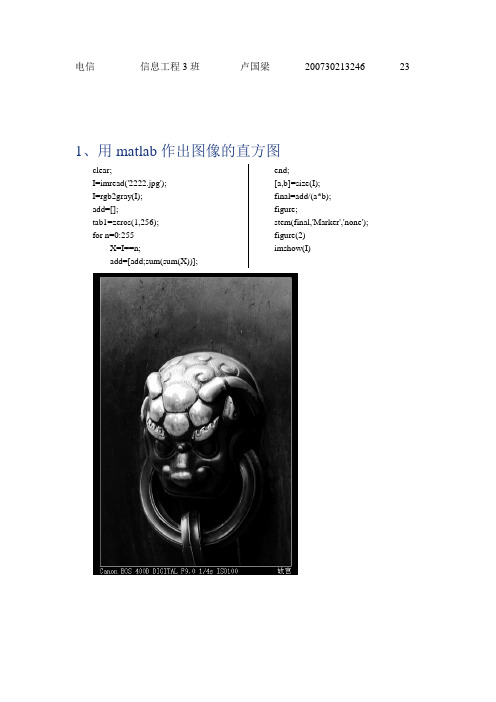
电信信息工程3班卢国梁200730213246 23 1、用matlab作出图像的直方图clear;I=imread('2222.jpg');I=rgb2gray(I);add=[];tab1=zeros(1,256);for n=0:255X=I==n;add=[add;sum(sum(X))]; end;[a,b]=size(I);final=add/(a*b);figure;stem(final,'Marker','none'); figure(2)imshow(I)2、用matlab实现图像的直方图均衡化均衡化前均衡化后程序:clear;I=imread('2222.jpg');I=rgb2gray(I);I2=I;add=[];add1=[];tab1=zeros(1,256);tab2=zeros(1,256);for n=0:255X=I==n;add=[add;sum(sum(X))]; end;[a,b]=size(I);final=add/(a*b);for n=1:256for i=1:ntab1(n)=tab1(n)+final(i);end;end;tab1=tab1*255;tab2=round(tab1); for n=1:afor m=1:bfor t=0:255if I(n,m)==tI2(n,m)=tab2(t+1);end;end;end;end;for n=0:255X1=I2==n;add1=[add1;sum(sum(X1))]; end;[a1,b1]=size(I2);final1=add1/(a1*b1);figure;stem(final,'Marker','none');figure(2)imshow(I2);figure(3)stem(final1,'Marker','none')均衡化后直方图实验心得体会:这次先是把老师的课件都看了一次,知道了各种方法,包括多幅图像去噪声啊,中值滤波啊等等,看了一些参考的程序,请教了同学,就写了这么几个程序,中间遇到了一些问题,比如在均衡化的时候判断的时候用错了序列,结果图像处理之后变得更加难看,思量着不可能越处理越糟糕,就里里外外看了好久的程序,毕竟是当局者,看不出来,请教了同学帮忙看错误,才找出了那个错误:if I(n,m)==add(t);I2(n,m)=tab2(t+1);后来改为if I(n,m)==t;I2(n,m)=tab2(t+1);图像也好看很多了!。
MATLAB直方图均衡化代码(MATLABhistogramequalizationcode)

MATLAB直方图均衡化代码(MATLAB histogram equalization code)Im = imread (' c: \ 1. JPG); The % file is called 1.jpg image, which is in the bottom of c disk, and of course the path can be changed by itselfIf size (im, 3) > 1 % determines if it is color image, convert to grayscaleIm = rgb2gray (im);Endhist_im = imhist (im); % computing hist_im; % draw histogram Close allI = imread (' C: \ Documents and Settings \ DMT \ desktop \ intern \ image \ gray image \ lenna.bmp ')Imshow (I);Imhist (I);The Matlab complete program of histogram and histogram equalization is 2010-06-04 15:43:10Classification:I. experimental purposeGrasp the basic image enhancement method, observe the effect of image enhancement, deepen the understanding of grayscale histogram and histogram equalization, and master the method ofhistogram equalization.Second, experimental contentConvert a color image into a gray image, paint grayscale histogram and equalization of the histogram, and compare the grayscale to the equalization.Third, the experimental principleThe grayscale histogram is to calculate the frequency of all pixels in the digital image according to the size of the gray value. Generally, the horizontal coordinates of the grayscale histogram indicate the gray value, the ordinate is the number of pixels, or the pixel value of a certain gray value can be used as the vertical coordinate.The basic principle of histogram equalization method is that the number of pixels in the image of grey value (that is, a major role on the image grey value) for broadening, and a small number of pixels of grey value (that is, does not play a major role on the picture of the grey value) to carry on the merge. To achieve the purpose of clear image.4. Experimental procedure% % % % % % % % % % % % % % % % % % % % % % % % % % % % % % % % % % % % % % % % % % % % % % % % % % % % % % % % % % % % % % % % % % % % % % % % % % %Function of % function, draw the histogram of the image, andmake histogram equalization to the image% direct read ABC. JPG, read to tuu% graydis is the number of grayscale pixels in the original histogram% primitive histogram graydispro, using the original histogram to calculate the original cumulative histogram graydisproThe new grayscale t [] calculated and the original grayscale corresponds to the new gray value t [], the mapping relationship is established, the t coordinates represent the original grayscale, and t [] represents the new coordinates corresponding to the original coordinates% new_graydis is the number of grayscale pixels of the new histogramThe new histogram new_graydispro is calculated and the new histogram new_graydispro is calculated using the new histogramThe new figure new_tu after the histogram equalization is calculated% % % % % % % % % % % % % % % % % % % % % % % % % % % % % % % % % % % % % % % % % % % % % % % % % % % % % % % % % % % % % % % % % % % % % % % % % % %Clear allClose allTuu = imread (' ABC. JPG); % read in picturesTu = rgb2gray (tuu); % converts color images to grayscaleGraydis = zeros (1256); % sets the matrix sizeGraydispro = zeros (1256);New_graydis = zeros (1256);New_graydispro = zeros (1256);H [w] = size (tu);New_tu = zeros (h, w);Graydis of grayscale pixels in the original histogram of the original histogramFor x = 1: hFor y = 1: wGraydis (1, tu (x, y)) = graydis (1, tu (x, y)) + 1;The endThe end% computing the original histogram graydisproGraydispro = graydis. / sum (graydis);Subplot (1, 2, 1);The plot (graydispro);Title (' grayscale histogram ');Xlabel (' gray value '); Ylabel (' pixel probability density ');Calculate the original cumulative histogram6 for I ="Graydispro (1, I) = graydispro (1, I) + graydispro (1, I - 1);The endThe new grayscale t [] with the corresponding % computation and the original grayscale is established to map the relationshipFor I = 25 JuneT (1, I) = floor (254 * graydispro (1, I) + 0.5);The end% statistics new histogram each grayscale pixel numbernew_graydisFor I = 25 JuneNew_graydis (1, t + 1) (1, I) = new_graydis (1, t (1, I) + 1) + graydis (1, I);The endCalculate the new grayscale histogram new_graydisproNew_graydispro = new_graydis. / sum (new_graydis);Subplot (1,2,2);The plot (new_graydispro);Title (" equalization of grayscale histogram ");Xlabel (' gray value '); Ylabel (' the probability density of pixels');The new figure new_tu after the histogram equalization is calculatedFor x = 1: hFor y = 1: wNew_tu (x, y) = t (1, tu (x, y));The endThe endFigure, imshow (tu, []);The title (' artwork ');Figure, imshow (new_tu, []);Title (' histogram equalization ');/ / / / / / / / / / / / / / / / / / / / / / / / / / / / / / / / / / / / / / / / / / / / / / / / / / / / / /The other two codes:codeMatlabThe following code is from archiless, which is very detailed and suitable for beginners.The % digital image processing program job% this program can grayscale and histogram equalization of JPG color image files%% input file: picsam.jpg for image processing% output file: PicSampleGray. BMP grayscale image% PicEqual. BMP equalization after image%% output graphical window descriptionThe color image is processed in % figure NO 1% figure NO 2 grayscale image% figure NO 3 histogram% figure NO 4 equalization of histogram% figure NO 5 greyscale% figure NO 6 equalization of the image% 1, the image you handle is picsam.jpg% 2, the program will clear the workspace every time it runs % the author; Archiless lorderClear all% 1, the image preprocessing, read into the color image to thegrayscalePS = imread (' PicSample. JPG);% read in JPG color image filesImshow (PS) % shows figure NO 1Title (' input color JPG image ')Imwrite (rgb2gray (PS), 'PicSampleGray. BMP); % color image grayscale and savePS = rgb2gray (PS); % grayscale data is stored in an arrayFigure, imshow (PS) % shows the grayscale image and the sample figure NO 2 before equalizationTitle (' grayscale image ')% 2 draw histogram[m, n] = size (PS); % measurement of image size parametersGP = zeros (1256); % precreate vectors that store probability of grayscaleFor k = 0:25 5GP (k + 1) = length (find (PS = = k))/(m * n); The probability of calculating the gray level of each level is calculated anddeposited into the corresponding position in the GPThe endFigure, bar (0:255, GP, 'g') % draw histogram figure NO 3 Title (' original image histogram ')Xlabel (' gray value ')Ylabel (' occurrence probability ')Third, the histogram equalizationS1 = zeros (1256);For I = 25 JuneFor j = 1: i.S1 (I) = GP (j) + S1 (I); % calculation SkThe endThe endS2 = round (S1 * 256); % return Sk to a similar level of grayscale For I = 25 JuneGPeq (I) = sum (GP (find (S2 = = I))); The probability of thepresent occurrence of each grayscale is calculatedThe endFigure, bar (0:25, GPeq, 'b') % display equalization of the histogram figure NO 4Title (histogram after equalization)Xlabel (' gray value ')Ylabel (' occurrence probability ')Figure, plot (0:25, S2, 'r') % display grayscale change curve figure NO 5Legend (' grayscale change curve ')Xlabel (' original image greyscale ')Ylabel (' post-equalization greyscale ')4. Image equalizationPA = PS;For I = 0:25 5PA (find (PS = = I)) = S2 (I + 1); % assigns each pixel to the pixel with a normalized gray valueThe endFigure, imshow (PA) % display equalization of the image figure NO 6Title (' equalized image ')Imwrite (PA, 'PicEqual. BMP);Another Matlab code, from histogram equalization - image enhancementI = imread (' LENA256. BMP);Imshow (I);Figure;Imhist (I);[m, n] = size (I);Hf = zeros (1256);Pa = zeros (1256);I = double (I);For I = 1: mFor j = 1: nHf (I + 1) (I, j) = hf (I (I, j) + 1) + 1; % statistics the number of grayscale pixelsThe endThe endBmap = zeros (1256);For I = 25 JuneTemp = 0;For j = 1: i.Temp = temp + hf (j);The endBmap (I) = floor (temp * 255 / (m * n));The endY = zeros (m, n);For I = 1: mFor j = 1: nY (I, j) = bmap (I (I, j) + 1);The endThe endY = uint8 (y);Figure;Imshow (y);Clear all;I = imread (' 1. JPG);I = rgb2gray (I); % gray,Make a histogram[m, n] = size (I);GP = zeros (1256);For k = 0:25 5GP (k + 1) = length (find) (I = = k)/(m * n); The probability of calculating the occurrence of grayscale at each level is deposited into GPThe endThird, the histogram equalizationS1 = zeros (1256);For I = 25 JuneFor j = 1: i.S1 (I) = GP (j) + S1 (I);The endThe endS2 = round (+ 0.5) * 256 (S1); % return Sk to a similar level of grayscaleFor I = 25 JuneGPeq (I) = sum (GP (find (S2 = = I))); The probability of the present occurrence of each grayscale is calculatedThe endFigure;Subplot (221); Bar (0:25 5, GP, 'b');Title (' original image histogram ')Subplot (222); Bar (0:25 5, GPeq, 'b')Title (histogram after equalization)X = I;For I = 0:25 5X (find (I = = I)) = S2 (I + 1);The endSubplot (223); Imshow (I);Title (' original image ');Subplot (224); Imshow (X);Title (' histogram equilibrium image ');。
matlab实验(直方图均衡化、频域锐化、空域锐化)
实验一直方图均衡化一、实验目的掌握基本的图象增强方法,观察图象增强的效果,加深对灰度直方图及直方图均衡化的理解,掌握直方图均衡化方法。
二、实验内容将一张彩色图片转换成灰色图片,做出均衡化后的直方图,并将灰度图和均衡化后的图片对比。
三、实验原理直方图均衡方法的基本原理是:对在图像中像素个数多的灰度值(即对画面起主要作用的灰度值)进行展宽,而对像素个数少的灰度值(即对画面不起主要作用的灰度值)进行归并。
从而达到清晰图像的目的。
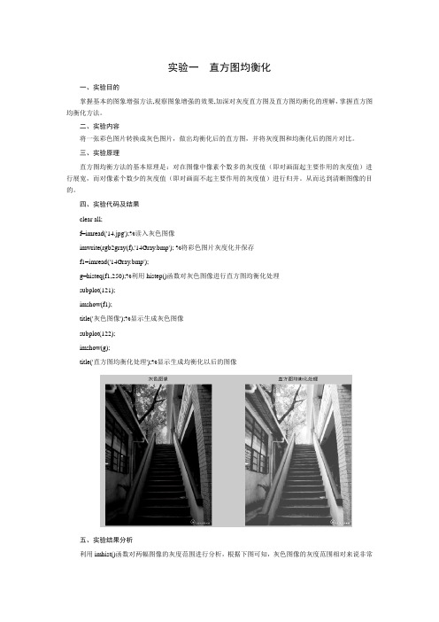
四、实验代码及结果clear all;f=imread('14.jpg');%读入灰色图像imwrite(rgb2gray(f),'14Gray.bmp'); %将彩色图片灰度化并保存f1=imread('14Gray.bmp');g=histeq(f1,250);%利用histep()函数对灰色图像进行直方图均衡化处理subplot(121);imshow(f1);title('灰色图像');%显示生成灰色图像subplot(122);imshow(g);title('直方图均衡化处理');%显示生成均衡化以后的图像五、实验结果分析利用imhist()函数对两幅图像的灰度范围进行分析,根据下图可知,灰色图像的灰度范围相对来说非常狭窄,图像质量比较差。
而经过直方图均衡化处理后,图像的对比度及平均亮度明显提高,直方图在整个亮度标度上明显扩展,图像质量明显提高。
实验二空域锐化一、实验目的理解图象锐化的概念,掌握常用空域锐化增强技术。
加深理解和掌握图像锐化的原理和具体算法,理解图象锐化增强的处理过程和特点。
二、实验内容利用一阶微分锐化增强,实现Roberts算子的锐化处理。
观察处理前后图像效果,分析实验结果和算法特点。
三、实验原理Roberts算子是突出图像的细节或者是增强被模糊了的细节。
因此要对图像实现锐化处理,可以用空间微分来完成,但是,这样图像的微分增强了边缘和其他的突变(如噪声)并削弱了灰度变化缓慢区域。
直方图均衡化matlab程序
直方图和直方图均衡的Matlab完整程序(数字图像处理)一、实验目的掌握基本的图象增强方法,观察图象增强的效果,加深对灰度直方图及直方图均衡化的理解,掌握直方图均衡化方法。
二、实验内容将一张彩色图片转换成灰色图片,画灰度直方图和均衡化后的直方图,并将灰度图和均衡化后的图片对比。
三、实验原理灰度直方图是将数字图像中的所有像素,按照灰度值的大小,统计其所出现的频度。
通常,灰度直方图的横坐标表示灰度值,纵坐标为像素个数,也可以采用某一灰度值的像素数占全图像素数的百分比作为纵坐标。
直方图均衡方法的基本原理是:对在图像中像素个数多的灰度值(即对画面起主要作用的灰度值)进行展宽,而对像素个数少的灰度值(即对画面不起主要作用的灰度值)进行归并。
从而达到清晰图像的目的。
四、实验程序%%%%%%%%%%%%%%%%%%%%%%%%%%%%%%%%%%%%%%%%%%%%%%%%% %%%%%%%%%%%%%%%%%%%%%%%%%%%函数功能,画出图像的直方图,并对图像进行直方图均衡%直接读图像abc.jpg,读到tuu中%graydis是原始直方图各灰度级像素个数%原始直方图graydispro,利用原始直方图计算原始累计直方图graydispro%t[]计算和原始灰度对应的新的灰度t[],建立映射关系,t坐标代表原始的灰度,t[]代表对应原始坐标的新坐标%new_graydis是统计新直方图各灰度级像素个数%计算新的灰度直方图new_graydispro,利用新的直方图计算新的累计直方图new_graydispro%计算直方图均衡后的新图new_tu %%%%%%%%%%%%%%%%%%%%%%%%%%%%%%%%%%%%%%%%%%%%%%%%% %%%%%%%%%%%%%%%%%%%%%%%%%%clear allclose alltuu=imread('abc.jpg'); %读入图片tu=rgb2gray(tuu); %将彩色图片转换为灰度图graydis=zeros(1,256); %设置矩阵大小graydispro=zeros(1,256);new_graydis=zeros(1,256);new_graydispro=zeros(1,256);[h w]=size(tu);new_tu=zeros(h,w);%计算原始直方图各灰度级像素个数graydisfor x=1:hfor y=1:wgraydis(1,tu(x,y))=graydis(1,tu(x,y))+1;endend%计算原始直方图graydisprograydispro=graydis./sum(graydis);subplot(1,2,1);plot(graydispro);title('灰度直方图');xlabel('灰度值');ylabel('像素的概率密度');%计算原始累计直方图for i=2:256graydispro(1,i)=graydispro(1,i)+graydispro(1,i-1); end%计算和原始灰度对应的新的灰度t[],建立映射关系for i=1:256t(1,i)=floor(254*graydispro(1,i)+0.5);end%统计新直方图各灰度级像素个数new_graydisfor i=1:256new_graydis(1,t(1,i)+1)=new_graydis(1,t(1,i)+1)+graydis(1,i); end%计算新的灰度直方图new_graydispronew_graydispro=new_graydis./sum(new_graydis);subplot(1,2,2);plot(new_graydispro);title('均衡化后的灰度直方图');xlabel('灰度值');ylabel('像素的概率密度');%计算直方图均衡后的新图new_tufor x=1:hfor y=1:wnew_tu(x,y)=t(1,tu(x,y));endendfigure,imshow(tu,[]);title('原图');figure,imshow(new_tu,[]);title('直方图均衡化后的图');//////////////////////////////////////////////////////另外两种代码:Matlab下面的代码来自archiless,注释非常详细,适合初学。
Matlab图像处理命令及实验程序
Matlab图像处理命令及实验程序图像增强1. 直方图均衡化的Matlab 实现1.1 imhist 函数功能:计算和显示图像的色彩直方图格式:imhist(I,n)imhist(X,map)说明:imhist(I,n) 其中,n 为指定的灰度级数目,缺省值为256;imhist(X,map) 就算和显示索引色图像X 的直方图,map 为调色板。
用stem(x,counts) 同样可以显示直方图。
1.2 imcontour 函数功能:显示图像的等灰度值图格式:imcontour(I,n),imcontour(I,v)说明:n 为灰度级的个数,v 是有用户指定所选的等灰度级向量。
1.3 imadjust 函数功能:通过直方图变换调整对比度格式:J=imadjust(I,[low high],[bottom top],gamma)newmap=imadjust(map,[low high],[bottom top],gamma)说明:J=imadjust(I,[low high],[bottom top],gamma) 其中,gamma 为校正量r,[low high] 为原图像中要变换的灰度范围,[bottom top]指定了变换后的灰度范围;newmap=imadjust(map,[low high],[bottom top],gamma) 调整索引色图像的调色板map 。
此时若[low high] 和[bottom top] 都为2×3的矩阵,则分别调整R、G、B 3个分量。
1.4 histeq 函数功能:直方图均衡化格式:J=histeq(I,hgram)J=histeq(I,n)[J,T]=histeq(I,...)newmap=histeq(X,map,hgram)newmap=histeq(X,map)[new,T]=histeq(X,...)说明:J=histeq(I,hgram) 实现了所谓“直方图规定化”,即将原是图象I 的直方图变换成用户指定的向量hgram 。
MATLAB图像处理-线性变换和直方图均衡
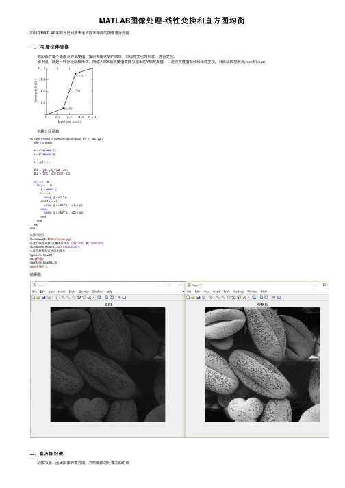
MATLAB图像处理-线性变换和直⽅图均衡如何在MATLAB中对于已经被表⽰成数字矩阵的图像进⾏处理⼀、灰度拉伸变换 把图像中每个像素点的灰度值,按照希望达到的效果,以线性变化的形式,进⾏变换。
如下图,就是⼀种分段函数形式,把输⼊的X轴灰度值变换为输出的Y轴灰度值,只是将灰度值做分段线性变换。
分段函数控制点(r1,s1)和(r2,s2) 创建分段函数: function [ new ] = StretchFunc(original, x1, y1, x2, y2 )new = original;w = size(new, 1);h = size(new, 2);k1 = y1 / x1;dk1 = (y2 - y1) / (x2 - x1);dk2 = (500 - y2) / (500 - x2);for i = 1 : wfor j = 1 : hx = new(i, j);if x < x1new(i, j) = k1 * x;elseif x < x2new(i, j) = dk1 * (x - x1) + y1;elsenew(i, j) = dk2 * (x - x2) + y2;endendendend%读⼊图⽚O=imread('F:\Maths\tupian.jpg');%进⾏线性变换,设置转折点为(200,100)和(300,400)NO=StretchFunc(O,200,100,300,400);%显⽰原图和变换后的图⽚figure,imshow(O);title('原图');figure,imshow(NO,[]);title('变换后');结果图:⼆、直⽅图均衡 函数功能,画出图像的直⽅图,并对图像进⾏直⽅图均衡 直接读图像tupian.jpg,读到O中 graydis是原始直⽅图各灰度级像素个数 原始直⽅图graydispro,利⽤原始直⽅图计算原始累计直⽅图graydispro t[]计算和原始灰度对应的新的灰度t[],建⽴映射关系,t坐标代表原始的灰度,t[]代表对应原始坐标的新坐标 new_graydis是统计新直⽅图各灰度级像素个数 计算新的灰度直⽅图new_graydispro,利⽤新的直⽅图计算新的累计直⽅图new_graydispro 计算直⽅图均衡后的新图NO%读⼊图⽚O=imread('F:\Maths\tupian.jpg');graydis=zeros(1,256); %设置矩阵⼤⼩graydispro=zeros(1,256);new_graydis=zeros(1,256);new_graydispro=zeros(1,256);[h w]=size(O);NO=zeros(h,w);%计算原始直⽅图各灰度级像素个数graydisfor x=1:hfor y=1:wgraydis(1,O(x,y))=graydis(1,O(x,y))+1;endend%计算原始直⽅图graydisprograydispro=graydis./sum(graydis);subplot(1,2,1);plot(graydispro);title('灰度直⽅图');xlabel('灰度值');ylabel('像素的概率密度');%计算原始累计直⽅图for i=2:256graydispro(1,i)=graydispro(1,i)+graydispro(1,i-1);end%计算和原始灰度对应的新的灰度t[],建⽴映射关系for i=1:256t(1,i)=floor(254*graydispro(1,i)+0.5);end%统计新直⽅图各灰度级像素个数new_graydisfor i=1:256new_graydis(1,t(1,i)+1)=new_graydis(1,t(1,i)+1)+graydis(1,i);end%计算新的灰度直⽅图new_graydispronew_graydispro=new_graydis./sum(new_graydis);subplot(1,2,2);plot(new_graydispro);title('均衡化后的灰度直⽅图');xlabel('灰度值');ylabel('像素的概率密度');%计算直⽅图均衡后的新图NOfor x=1:hfor y=1:wNO(x,y)=t(1,O(x,y));endendfigure,imshow(O);title('原图');figure,imshow(NO,[]);title('直⽅图均衡化后的图'); 结果:。
matlab 直方图均衡实验报告

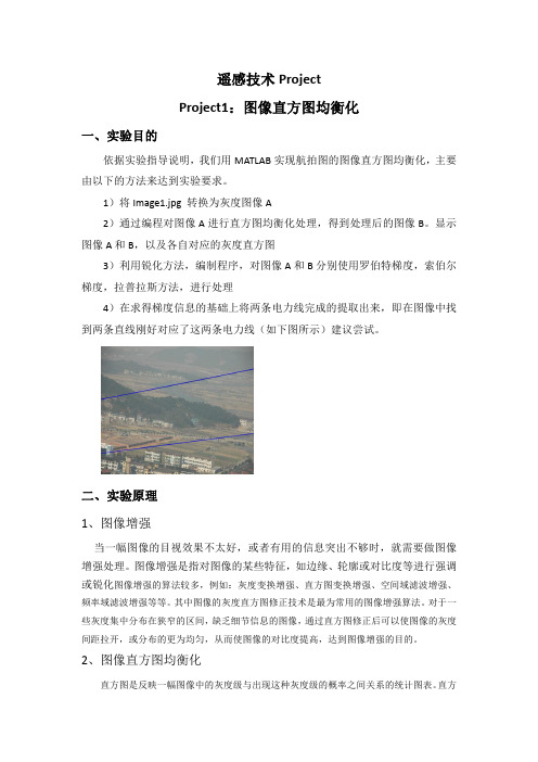
基于直方图的灰度级修正班级:电子信息科学与技术0901班姓名:学号:设计时间: 2012年5月24日一 设计课题:基于直方图的灰度级修正二 设计内容及要求:实验原理: 1.直方图均衡化处理技术是用累积分布函数作变换函数的直方图修正方法;2.用累积分布函数作为变换函数可产生一幅灰度级分布具有均匀概率密度的图像。
均衡步骤:1、统计原始图像的直方图,求出)(k r r P ;2、用累积分布函数作变换∑==kj j r k r P s 0)( ,求变换后的新灰度;3、用新灰度代替旧灰度,求出)(k s s P ,这一步是近似的,力求合理,同时把灰度相等的或相近的合在一起。
设计要求:1. 利用fopen 等函数打开*.dat 文件,采用for 循环统计图像里各灰度级的个数,并用换图函数表示出来。
2. 将打开的图像,采用直方图均衡对原始图像进行灰度级转换,并绘出其灰度直方图。
三 程序设计及其说明:本程序采用matlab GUI 绘图来实现,操作界面、菜单内容如下:图1 操作界面图2 菜单内容程序特色:1.原始图像灰度直方图统计算法一for l=0:255for i=1:rowif fid(i,1)==lh(l+1)=h(l+1)+1;endendend2. 原始图像灰度直方图统计算法二for i=1:rowh(fid(i)+1)=h(fid(i)+1)+1;end由主要代码部分可以看出:算法二算法复杂度很小,这是利用fopen打开文件的特色来决定的,它读入数组时是m行1列。
四实验结果及分析:灰度直方图统计:原始图像与均衡后图像灰度直方图(以LENA女孩图像为例)不同亮度图像直方图均衡效果显示1. LENA 图像 (1)正常图5 LENA 正常 原始及均衡后图像显示(2)高亮度图3 原始图像直方图图4 图像均衡后直方图图6 LENA高光原始及均衡后图像显示(3)偏暗图7 LENA偏暗原始及均衡后图像显示2.couple图像(1)正常图8 couple正常原始及均衡后图像显示图9 couple高亮原始及均衡后图像显示(3)偏暗图10 couple偏暗原始及均衡后图像显示3.NBA图像(1)正常图11 NBA正常原始及均衡后图像显示(3)偏暗图13 NBA偏暗原始及均衡后图像显示不同亮度的原始图像与均衡后图像灰度直方图1. LENA图像(1)正常(2)高亮度(3)偏暗图16 原始图像直方图图17 图像均衡后直方图图14 原始图像直方图图15 图像均衡后直方图2. couple 图像 (1)正常(2)高亮度图20 原始图像直方图图21 图像均衡后直方图图18 原始图像直方图图19 图像均衡后直方图(3)偏暗3. NBA 图像 (1)正常图24 原始图像直方图图25 图像均衡后直方图图22 原始图像直方图图23 图像均衡后直方图(2)高亮度(3)偏暗图28 原始图像直方图图29 图像均衡后直方图图26 原始图像直方图图27 图像均衡后直方图结果分析:通过几个图像显示结果可以看出:直方图均衡结果使图像亮度有所提高,所以它对比较暗的图像显示的更加清晰,而太亮的图像或曝光过度的图像,经过直方图均衡,效果不是很好,但是轮廓勾画的会明显些。
直方图均衡化的MATLAB实现(遥感课程设计)
s T r Pr r dr
0
(2.4)
其中,
P r dr 是 r 的累积分布函数,由于累积分布函数是 r 的函数,且从 0 到 1 单调递
0 r
r
增,所以变换函数即式(2.4)满足关于 T r 在 0 r 1 区间内单值单调增加,在 0 r 1 内有 0 T r 1 的两个条件。 对公式(2.4)中的 r 求导,有 ds / dr Pr r ,把求导结果代入式(2.3),则有:
2、图像直方图均衡化
直方图是反映一幅图像中的灰度级与出现这种灰度级的概率之间关系的统计图表。 直方
图的横坐标是灰度级 rk , 纵坐标是图像中具有该灰度级的像素个数或出现这个灰度级数的概 率 P rk 。直方图能直观地表示出图像具有某种灰度级的像素个数,是对图像灰度值分布情 总数, nk 为第 k 级灰度的像素数。 通过观察图像的灰度直方图, 就可以判断这幅图像的对比度和清晰度, 也可以掌握图像 的明暗程度。本文即采用直方图均衡化[11]的方法来对航拍图像进行增强处理。 设 r 和 s 分别表示归一化 (注: 归一化是指图像的灰度值通过某个比例变换后限制在[0,1] 之间)的图像灰度和经直方图修正后的图像灰度,即 0 r , s 1 。在 0,1 区间内的任何一 个 r 值都可产生一个 s 值,且有: s T r 。T r 为变换函数,满足:(1)在 0 r 1 区 间内是单调递增函数;(2)对于 0 r 1 ,有 0 T r 1 。条件(1)保证变换后的灰度 从黑到白的次序不变,条件(2)确保灰度变换后的像素处于允许的范围之内。从 s 到 r 的 反变换关系为: r T 况的整体描述。概率灰度直方图的计算公式为: P rk nk / N 。其中 N 为图像中的像素
matlab直方图修正
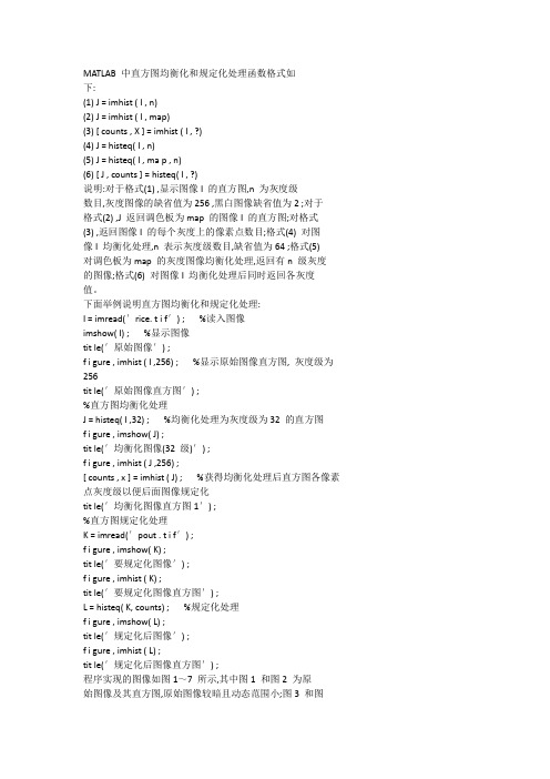
MATLAB 中直方图均衡化和规定化处理函数格式如下:(1) J = imhist( I , n)(2) J = imhist( I , map)(3) [ counts , X ] = imhist ( I , ?)(4) J = histeq( I , n)(5) J = histeq( I , ma p , n)(6) [ J , counts ] = histeq( I , ?)说明:对于格式(1) ,显示图像I 的直方图,n 为灰度级数目,灰度图像的缺省值为256 ,黑白图像缺省值为2 ;对于格式(2) ,J 返回调色板为map 的图像I 的直方图;对格式(3) ,返回图像I 的每个灰度上的像素点数目;格式(4) 对图像I 均衡化处理,n 表示灰度级数目,缺省值为64 ;格式(5)对调色板为map 的灰度图像均衡化处理,返回有n 级灰度的图像;格式(6) 对图像I 均衡化处理后同时返回各灰度值。
下面举例说明直方图均衡化和规定化处理:I = imread(′rice. t i f′) ; %读入图像imshow( I) ; %显示图像tit le(′原始图像′) ;f igure , imhist ( I ,256) ; %显示原始图像直方图, 灰度级为256tit le(′原始图像直方图′) ;%直方图均衡化处理J = histeq( I ,32) ; %均衡化处理为灰度级为32 的直方图figure , imshow( J) ;tit le(′均衡化图像(32 级)′) ;figure , imhist ( J ,256) ;[ counts , x ] = imhist ( J) ; %获得均衡化处理后直方图各像素点灰度级以便后面图像规定化tit le(′均衡化图像直方图1′) ;%直方图规定化处理K = imread(′pout . t i f′) ;figure , imshow( K) ;tit le(′要规定化图像′) ;figure , imhist ( K) ;tit le(′要规定化图像直方图′) ;L = histeq( K, counts) ; %规定化处理figure , imshow( L) ;tit le(′规定化后图像′) ;figure , imhist ( L) ;tit le(′规定化后图像直方图′) ;程序实现的图像如图1~7 所示,其中图1 和图2 为原始图像及其直方图,原始图像较暗且动态范围小;图3 和图4 分别是对原始图像进行灰度级为32 级的均衡化处理的结果,可以看到处理后图像亮度值出现的频数趋于平衡,灰度的动态范围和对比度差都得到了增强;图5 和图6 为需要规定化处理的图像及其直方图;图7 和图8 是采用直方图规定化处理后的结果,可以看到规定化处理将原来较暗区域的一些细节得到增强而变得更加清晰了。
MATLAB直方图均衡化代码
I = imread('C:\Documents and Settings\dmt\桌面\实习\图像\灰度图像\lenna.bmp')
imshow(I);
imhist(I);
直方图和直方图均衡的Matlab完整程序 2010-06-04 15:43:10
title('灰度化后的图像')
%二,绘制直方图
[m,n]=size(PS); %测量图像尺寸参数
GP=zeros(1,256); %预创建存放灰度出现概率的向量
for k=0:255
y(i,j)=bmap(I(i,j)+1);
end
end
y=uint8(y);
figure;
imshow(y);
clear all;
I = imread('1.jpg');
I=rgb2gray(I); %灰度化
%绘制直方图
[m,n]=size(I);
GP=zeros(1,256);
for k=0:255
GP(k+1)=length(find(I==k))/(m*n); %计算每级灰度出现的概率,将其存入GP
end
%三,直方图均衡化
S1=zeros(1,256);
for i=1:256
temp=0;
for j=1:i
temp=temp+hf(j);
end
bmap(i)=floor(temp*255/(m*n));
end
y=zeros(m,n);
for i=1:m
for j=1:n
直方图均衡化matlab代码

图片采用了维基百科直方图均衡化中的图片保存为文件名test0.jpg直方图均衡化的原理参考《数字图像处理第三版(冈萨雷斯)》第75页公式3.3-8(主要就是一个公式)代码如下:imgdat0=imread('test0.jpg');%读图[r,c]=size(imgdat0);%图像尺寸PixelNum=r*c;%图像尺寸distribute=zeros(1,256);%原始直方图统计for i=1:PixelNumpos=imgdat0(i)+1;%加1是因为matlab索引从1开始而不是从0开始distribute(pos)=distribute(pos)+1;%pos为像素值,范围0-255/1-256enddistribute=distribute/PixelNum;%原始直方图统计convertarray=zeros(1,256);%像素转换对应tempadd=0;%累加计算使用for i=1:255%计算像素转换对应公式tempadd=tempadd+distribute(i);convertarray(i)=uint8(255*tempadd);endrimgdat0=uint8(zeros(r,c));%计算结果图像for i=1:PixelNumrimgdat0(i)=convertarray(imgdat0(i));%像素值转换end%显示figureimshow(imgdat0)figureimshow(rimgdat0)figurebar(distribute)rdistribute=zeros(1,256);%计算结果直方图统计for i=1:PixelNumpos=rimgdat0(i)+1;rdistribute(pos)=rdistribute(pos)+1;endfigurebar(rdistribute)原图结果图计算前后的直方图。
matlab的histeq函数

Matlab的histeq函数1. 简介histeq函数是Matlab中用于直方图均衡化的函数。
直方图均衡化是一种图像增强的技术,它通过调整图像的灰度级分布,使得图像的对比度增加,细节更加清晰。
2. 直方图均衡化原理直方图均衡化的原理基于对图像的像素值进行变换,以实现灰度级分布的改变。
具体步骤如下:1.统计原始图像中每个灰度级的像素个数,得到灰度级直方图。
2.计算原始图像的累积分布函数(CDF),即每个灰度级的累积像素个数。
3.通过将CDF进行归一化,得到灰度级分布的概率密度函数(PDF)。
4.对于每个输入像素,将其映射到新的灰度级,即将原始的CDF值映射到0到255的范围内。
5.得到均衡化后的图像。
3. histeq函数的使用方法histeq函数的基本语法如下:J = histeq(I)其中,I为输入的灰度图像,J是经过直方图均衡化处理后的输出图像。
4. histeq函数的参数histeq函数还可以通过一些参数来进一步控制直方图均衡化的效果。
常用的参数包括:•numbins:用于计算灰度直方图的bin数,默认为256。
•mask:用于指定ROI(感兴趣区域)的二进制掩码图像。
•n:用于指定直方图均衡化的迭代次数,默认为1。
5. 示例以下是一个示例,演示了如何使用histeq函数对图像进行直方图均衡化:I = imread('lena.jpg');J = histeq(I);imshowpair(I, J, 'montage')上述代码会加载一张名为lena.jpg的图像,然后对其进行直方图均衡化处理,并显示原始图像和均衡化后的图像对比。
6. 直方图均衡化的效果直方图均衡化能够显著改善图像的对比度,并提升图像细节的可见性。
它在各种图像处理任务中都有广泛的应用,例如图像增强、边缘检测和目标识别等。
7. 结论通过本文对Matlab的histeq函数进行了详细的介绍,包括其原理、使用方法和参数。
实验3 图像的直方图均衡化
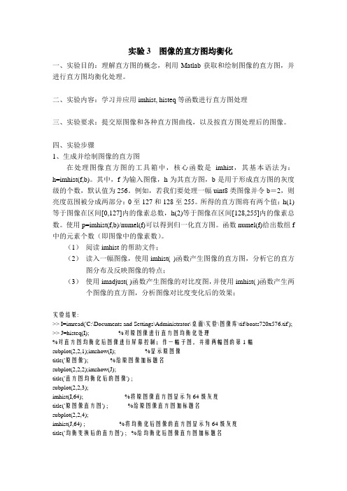
实验3 图像的直方图均衡化一、实验目的:理解直方图的概念,利用Matlab获取和绘制图像的直方图,并进行直方图均衡化处理。
二、实验内容:学习并应用imhist, histeq等函数进行直方图处理三、实验要求:提交原图像和各种直方图曲线,以及按直方图处理后的图像。
四、实验步骤1、生成并绘制图像的直方图在处理图像直方图的工具箱中,核心函数是imhist,其基本语法为:h=imhist(f,b)。
其中,f为输入图像,h为其直方图,b是用于形成直方图的灰度级的个数,默认值为256。
例如,若我们要处理一幅uint8类图像并令b=2,则亮度范围被分成两部分:0至127和128至255。
所得的直方图将有两个值:h(1)等于图像在区间[0,127]内的像素总数,h(2)等于图像在区间[128,255]内的像素总数。
使用p=imhist(f,b)/numel(f)可以得到归一化直方图。
函数numel(f)给出数组f 中的元素个数(即图像中的像素数)。
(1)阅读imhist的帮助文件;(2)读入一幅图像,使用imhist( )函数产生图像的直方图,分析它的直方图分布及反映图像的特点;(3)使用imadjust( )函数产生图像的对比度图,并使用imhist( )函数产生两个图像的直方图,分析图像对比度变化后的效果;实验结果:>> I=imread('C:\Documents and Settings\Administrator\桌面\实验\图像库\tif\boats720x576.tif'); >> J=histeq(I); %对原图像进行直方图均衡化处理%对直方图均衡化后图像进行屏幕控制;作一幅子图,并排两幅图的第1幅subplot(2,2,1);imshow(I); %显示原图像title('原图像'); %给原图像加标题名subplot(2,2,2);imshow(J);title('直方图均衡化后的图像') ;subplot(2,2,3);imhist(I,64); %将原图像直方图显示为64级灰度title('原图像直方图') ; %给原图像直方图加标题名subplot(2,2,4);imhist(J,64) ; %将均衡化后图像的直方图显示为64级灰度title('均衡变换后的直方图') ; %给均衡化后图像直方图加标题名原图像直方图均衡化后的图像01002004原图像直方图0100200050001000015000均衡变换后的直方图2、直方图均衡化直方图均衡化由工具箱中的函数histeq 实现,该函数语法为g=histeq(f,nlev)。
用MATLAB统计图像直方图

f (m,n)
f (1,0)
f (1,1)
f (1, N 1)
f(m,n)
f
(M
1,0)
f (M 1,1)
f (M 1, N 1)
m
编程思想
1、读入图像,cห้องสมุดไป่ตู้meraman.tif,并显示
2、获取图像空间坐标,灰度范围 3、统计各个灰度的像素个数 4、绘制直方图
绘图:plot(x,y) x = -pi:pi/10:pi; y = tan(sin(x)) - sin(tan(x)); plot(x,y,'--rs','LineWidth',2,...
用MATLAB统计图像直方图
安玉磊
基本概念
灰度直方图:数字图像中各灰度级与其出现的概 率的统计关系。可以表示为
p(i) ni ,i 0,1,2...L 1 n
且满足
L 1
p(i)
n L1 i
1
i0
i0 n
基本概念
数字图像的矩阵存储格式
O n
f (0,0) f (0,1) f (0, N 1)
5
1
上机一
熟悉MatLab环境及基本操作 作业
1、图像的基本操作
读图像文件及显示图像
2、绘制图像的直方图及直方图均衡变换
自己编程求解图像的直方图
3、自己退化一幅图像,并用维纳滤波复原
1、无噪声 2、有噪声
IJ KL
4.2 图像的直方图修正
•步
骤
•计算方法或公式
•1 •列出图像灰度级(i或j)
•2 •统计原图像各灰度级像素个数ni
•3
计算原始直方图:
- 1、下载文档前请自行甄别文档内容的完整性,平台不提供额外的编辑、内容补充、找答案等附加服务。
- 2、"仅部分预览"的文档,不可在线预览部分如存在完整性等问题,可反馈申请退款(可完整预览的文档不适用该条件!)。
- 3、如文档侵犯您的权益,请联系客服反馈,我们会尽快为您处理(人工客服工作时间:9:00-18:30)。
自己编的代码
Matlab中自带的函数
clc;clear all;
%用自己编的函数
pic1=imread('188_2.jpg');%修改数字可以看到另一幅图片的效果pic1=rgb2gray(pic1);
subplot(221);imshow(pic1);title('均衡化前的图像'); subplot(222);imhist(pic1);title('均衡化前的直方图');
L=256;%设置灰度级为256
[width,height]=size(pic1);
%求nk
nk=zeros(1,L);
for i=0:L-1
num=find(pic1==(i+1));
nk(i+1)=length(num);
end
%求pr(rk)=nk/MN
pr=zeros(1,L);
for i=1:L
pr(i)=nk(i)/(width*height);
end
%pc存储的就是累计的归一化直方图
pc=zeros(1,L);
for i=1:L
for j=1:i
pc(i)=pc(i)+pr(j);
end
end
sk=zeros(1,L);
for i=1:L
sk(i)=round((L-1)*pc(i));
end
%求pr(sk),即计算现有每个灰度级出现的概率并显示在屏幕上for i=0:L-1
pr(i+1)=sum(pc(find(sk==i)));
end
pr %显示pr值
%替换原有图片
pic2=pic1;
for i=1:L
pic2(find(pic2==(i-1)))=sk(i);
end
subplot(223);imshow(pic2);title('均衡化后的图像'); subplot(224);imhist(pic2);title('均衡化后的直方图');
%用matlab自带的函数
pic1=imread('188_2.jpg');%先把要处理的图像读入
pic1=rgb2gray(pic1);%转化成灰度图像
%显示灰度图像与直方图
figure;
subplot(221);imshow(pic1);title('均衡化前的图像'); subplot(222);imhist(pic1);title('均衡化前的直方图');
%直方图均衡化
pic2=histeq(pic1);
subplot(223);imshow(pic2);title('均衡化后的图像'); subplot(224);imhist(pic2);title('均衡化后的直方图');。