数字信号处理实验2 答案
数字信号处理第2章答案 史林 赵树杰编著
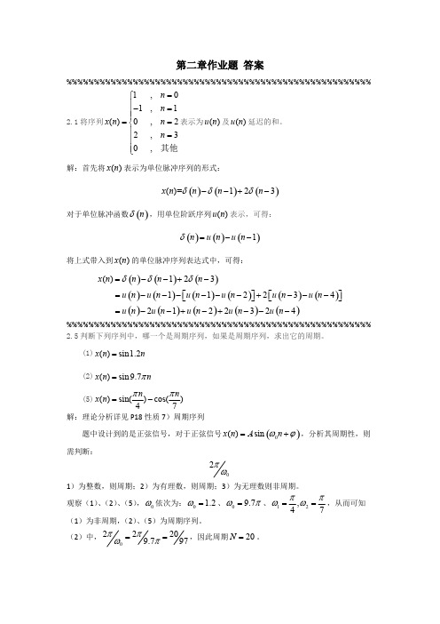
第二章作业题 答案%%%%%%%%%%%%%%%%%%%%%%%%%%%%%%%%%%%%%%%%%%%%%%%%%%%%%%%2.1将序列1,01,1()0,22,30,n n x n n n =⎧⎪-=⎪⎪==⎨⎪=⎪⎪⎩其他表示为()u n 及()u n 延迟的和。
解:首先将表示为单位脉冲序列的形式:()x n ()()()()=123x n n n n δδδ--+-对于单位脉冲函数,用单位阶跃序列表示,可得:()n δ()u n ()()()1n u n u n δ=--将上式带入到的单位脉冲序列表达式中,可得:()x n ()()()()()()()()()()()()()()()1231122342122324x n n n n u n u n u n u n u n u n u n u n u n u n u n δδδ=--+-=------+---⎡⎤⎡⎤⎣⎦⎣⎦=--+-+---%%%%%%%%%%%%%%%%%%%%%%%%%%%%%%%%%%%%%%%%%%%%%%%%%%%%%%%2.5判断下列序列中,哪一个是周期序列,如果是周期序列,求出它的周期。
(1)()sin1.2x n n =(2)()sin 9.7x n n π=(5)()sin()cos()47nnx n ππ=-解:理论分析详见P18性质7)周期序列题中设计到的是正弦信号,对于正弦信号,分析其周期性,则()0()sin x n A n ωϕ=+需判断:2πω1)为整数,则周期;2)为有理数,则周期;3)为无理数则非周期。
观察(1)、(2)、(5),依次为:、、,从而可知0ω0 1.2ω=09.7ωπ=12,47ππωω==(1)为非周期,(2)、(5)为周期序列。
(2)中,,因此周期。
022209.797ππωπ==20N =(5)中,第一部分周期为,第二部分周期为,因此序列1028N πω==20214N πω==周期为。
数字信号处理实验答案
实验一熟悉Matlab环境一、实验目的1.熟悉MATLAB的主要操作命令。
2.学会简单的矩阵输入和数据读写。
3.掌握简单的绘图命令。
4.用MATLAB编程并学会创建函数。
5.观察离散系统的频率响应。
二、实验内容认真阅读本章附录,在MATLAB环境下重新做一遍附录中的例子,体会各条命令的含义。
在熟悉了MATLAB基本命令的基础上,完成以下实验。
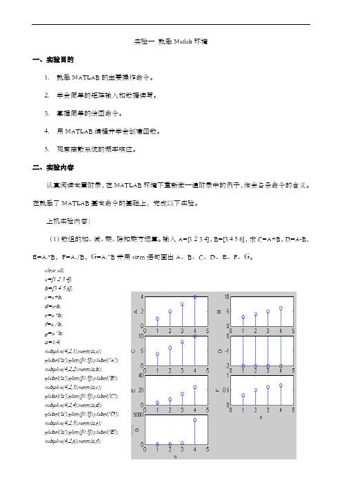
上机实验内容:(1)数组的加、减、乘、除和乘方运算。
输入A=[1 2 3 4],B=[3 4 5 6],求C=A+B,D=A-B,E=A.*B,F=A./B,G=A.^B并用stem语句画出A、B、C、D、E、F、G。
clear all;a=[1 2 3 4];b=[3 4 5 6];c=a+b;d=a-b;e=a.*b;f=a./b;g=a.^b;n=1:4;subplot(4,2,1);stem(n,a);xlabel('n');xlim([0 5]);ylabel('A');subplot(4,2,2);stem(n,b);xlabel('n');xlim([0 5]);ylabel('B');subplot(4,2,3);stem(n,c);xlabel('n');xlim([0 5]);ylabel('C');subplot(4,2,4);stem(n,d);xlabel('n');xlim([0 5]);ylabel('D');subplot(4,2,5);stem(n,e);xlabel('n');xlim([0 5]);ylabel('E');subplot(4,2,6);stem(n,f);xlabel('n');xlim([0 5]);ylabel('F');subplot(4,2,7);stem(n,g);xlabel('n');xlim([0 5]);ylabel('G');(2)用MATLAB实现下列序列:a) x(n)=0.8n0≤n≤15b) x(n)=e(0.2+3j)n0≤n≤15c) x(n)=3cos(0.125πn+0.2π)+2sin(0.25πn+0.1π) 0≤n≤15d) 将c)中的x(n)扩展为以16为周期的函数x16(n)=x(n+16),绘出四个周期。
数字信号处理 答案 第二章(精编文档).doc

【最新整理,下载后即可编辑】第二章2.1 判断下列序列是否是周期序列。
若是,请确定它的最小周期。
(1)x(n)=Acos(685ππ+n )(2)x(n)=)8(π-ne j (3)x(n)=Asin(343ππ+n )解 (1)对照正弦型序列的一般公式x(n)=Acos(ϕω+n ),得出=ω85π。
因此5162=ωπ是有理数,所以是周期序列。
最小周期等于N=)5(16516取k k =。
(2)对照复指数序列的一般公式x(n)=exp[ωσj +]n,得出81=ω。
因此πωπ162=是无理数,所以不是周期序列。
(3)对照正弦型序列的一般公式x(n)=Acos(ϕω+n ),又x(n)=Asin(343ππ+n )=Acos(-2π343ππ-n )=Acos(6143-n π),得出=ω43π。
因此382=ωπ是有理数,所以是周期序列。
最小周期等于N=)3(838取k k =2.2在图2.2中,x(n)和h(n)分别是线性非移变系统的输入和单位取样响应。
计算并列的x(n)和h(n)的线性卷积以得到系统的输出y(n),并画出y(n)的图形。
(a)1111(b)(c)111110 0-1-1-1-1-1-1-1222222 3333444………nnn nnnx(n)x(n)x(n)h(n)h(n)h(n)21u(n)u(n)u(n)a n ===22解 利用线性卷积公式y(n)=∑∞-∞=-k k n h k x )()(按照折叠、移位、相乘、相加、的作图方法,计算y(n)的每一个取样值。
(a) y(0)=x(O)h(0)=1y(l)=x(O)h(1)+x(1)h(O)=3y(n)=x(O)h(n)+x(1)h(n-1)+x(2)h(n-2)=4,n ≥2 (b) x(n)=2δ(n)-δ(n-1)h(n)=-δ(n)+2δ(n-1)+ δ(n-2) y(n)=-2δ(n)+5δ(n-1)= δ(n-3) (c) y(n)= ∑∞-∞=--k kn k n u k u a)()(=∑∞-∞=-k kn a=aa n --+111u(n)2.3 计算线性线性卷积 (1) y(n)=u(n)*u(n) (2) y(n)=λn u(n)*u(n)解:(1) y(n)=∑∞-∞=-k k n u k u )()( =∑∞=-0)()(k k n u k u =(n+1),n ≥0 即y(n)=(n+1)u(n)(2) y(n)=∑∞-∞=-k k k n u k u )()(λ=∑∞=-0)()(k kk n u k u λ=λλ--+111n ,n ≥0即y(n)=λλ--+111n u(n)2.4 图P2.4所示的是单位取样响应分别为h 1(n)和h 2(n)的两个线性非移变系统的级联,已知x(n)=u(n), h 1(n)=δ(n)-δ(n-4), h 2(n)=a n u(n),|a|<1,求系统的输出y(n).解ω(n)=x(n)*h1(n)=∑∞-∞=k ku)([δ(n-k)-δ(n-k-4)] =u(n)-u(n-4)y(n)=ω(n)*h2(n)=∑∞-∞=k k k ua)([u(n-k)-u(n-k-4)]=∑∞-=3nk ka,n≥32.5 已知一个线性非移变系统的单位取样响应为h(n)=a n-u(-n),0<a<1 用直接计算线性卷积的方法,求系统的单位阶跃响应。
数字信号处理II习题解答-2004(老师版)精选全文
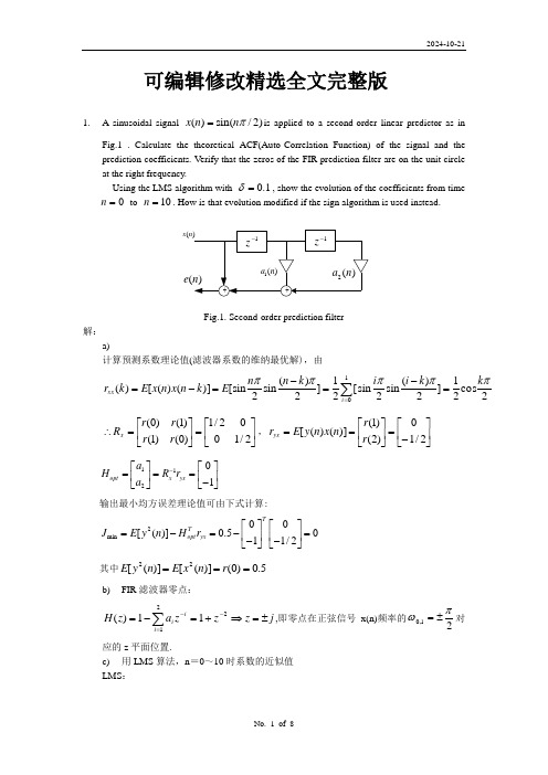
可编辑修改精选全文完整版1. A sinusoidal signal )2/sin()(πn n x =is applied to a second-order linear predictor as inFig.1 . Calculate the theoretical ACF(Auto-Correlation Function) of the signal and the prediction coefficients. Verify that the zeros of the FIR prediction filter are on the unit circle at the right frequency.Using the LMS algorithm with 1.0=δ, show the evolution of the coefficients from time 0=n to 10=n . How is that evolution modified if the sign algorithm is used instead.(n x (e Fig.1. Second-order prediction filter解:a)计算预测系数理论值(滤波器系数的维纳最优解),由2cos21]2)(sin 2sin [21]2)(sin 2[sin )]()([)(10πππππk k i i k n n E k n x n x E k r i xx =-=-=-=∑=⎥⎦⎤⎢⎣⎡=⎥⎦⎤⎢⎣⎡=∴2/1002/1)0()1()1()0(r r r r R x ,⎥⎦⎤⎢⎣⎡-=⎥⎦⎤⎢⎣⎡==2/10)2()1()]()([r r n x n y E r yx11201opt x yx a H R r a -⎡⎤⎡⎤===⎢⎥⎢⎥-⎣⎦⎣⎦输出最小均方误差理论值可由下式计算:2min00[()]0.5011/2TTopt yx J E y n H r ⎡⎤⎡⎤=-=-=⎢⎥⎢⎥--⎣⎦⎣⎦其中5.0)0()]([)]([22===r n x E n y E b) FIR 滤波器零点:j z z z a z H i i i ±=⇒+=-=-=-∑22111)(,即零点在正弦信号x(n)频率的21,0πω±=对应的z 平面位置.c) 用LMS 算法,n =0~10时系数的近似值 LMS :⎩⎨⎧+-+=++++=+)1()()1()1()1()1()()1(n X n H n y n e n e n X n H n H Tδ 在线性预测误差滤波的LMS 算法中:)1()1()]1(),([)()1()](),([)()(21+⇒+-=⇒+=⇒n x n y n x n x n X n X n a n a n A n H T T⎩⎨⎧-+=+++=+)()()1()1()1()()()1(n X n A n x n e n e n X n A n A Tδ ()⎪⎩⎪⎨⎧=<==TA n n x n n x ]0,0[)0(0,0)(),2sin()(π所以, LMS 算法下的预测误差滤波器[]⎪⎪⎩⎪⎪⎨⎧⎥⎦⎤⎢⎣⎡-++⎥⎦⎤⎢⎣⎡=⎥⎦⎤⎢⎣⎡++⎥⎦⎤⎢⎣⎡--+=+)1()()1()()()1()1()1()()()()1()1(212121n x n x n e n a n a n a n a n x n x n a n a n x n e δ 344.00344.00729.027.00027.0081.019.00019.009.01.0001.0010)2(0)2(0)2()2(20)1(0)1(1)1()1(10)0(0)0(0212121----------============= a a x e n a a x e n a a n d) 符号算法[]⎪⎪⎩⎪⎪⎨⎧⎥⎦⎤⎢⎣⎡-++⎥⎦⎤⎢⎣⎡=⎥⎦⎤⎢⎣⎡++⎥⎦⎤⎢⎣⎡--+=+)1()()]1([)()()1()1()1()()()()1()1(212121n x n x sign n e sign n a n a n a n a n x n x n a n a n x n e δ )()]([0,1)(n x n x sign n x =∴±=4.004.007.03.0003.008.02.0002.009.01.0001.0010)2(0)2(0)2()2(20)1(0)1(1)1()1(10)0(0)0(0212121----------============= a a x e n a a x e n a a n2. A second-order adaptive FIR filter has the input as )2/sin()(πn n x = and)2(5.0)1()()(-+-+=n x n x n x n yas reference signal. Calculate the coefficients, starting from zero initial values, from time n=0 to n = 10 . Calculate the theoretical residual error and the time constant and compare with the experimental results.()1.0=δ 解:取1.0=δa) 计算n =0~10的系数⎪⎩⎪⎨⎧+++=++-+=+-+-+=)3()1()1()()1()2()1()()1()1()1()2(5.0)1()()(n e n X n H n H n X n H n y n e n x n x n x n y Tδ 2cos 21)(πk k r xx =⎥⎦⎤⎢⎣⎡=⎥⎦⎤⎢⎣⎡=2/1002/1)0()1()1()0(r r r r R x ,⎥⎦⎤⎢⎣⎡=⎥⎦⎤⎢⎣⎡++++=2/14/1)1(5.0)0()1()2(5.0)1()0(r r r r r r r yx①⎥⎦⎤⎢⎣⎡==-12/11yx x opt r R H 2min [()]Topt yx J E y n H r =-⎥⎦⎤⎢⎣⎡⎥⎦⎤⎢⎣⎡--+--+-+-+-+=2/14/112/1)]2()()2()1()1()(2)2(25.0)1()([222Tn x n x n x n x n x n x n x n x n x E08/5)2()1(3)0(25.2=-++=r r r②Theoretical residual error: 0)21()(2min =+≈∞⇒∞σδN J J③Theoretical time constant :2211111120 (,)(0)0.10.5N e k x k x k x R r N τλλσλδλδσδ=≈======⨯∑是特征值 注意: 由于均方收敛的时间常数比均值收敛的时间常数小, 所以实际应用中采用较保守的理论估计值,即采用均值收敛的时间常数作为算法收敛的时间常数的理论估计值. ④利用(2)(3)作迭代:)0(0)(<=n n x ,0)0()0(21==h h[]⎪⎪⎩⎪⎪⎨⎧⎥⎦⎤⎢⎣⎡+++⎥⎦⎤⎢⎣⎡=⎥⎦⎤⎢⎣⎡++⎥⎦⎤⎢⎣⎡+-+=+)()1()1()()()1()1()()1()()()1()1(212121n x n x n e n h n h n h n h n x n x n h n h n y n e δ )1(5.0)()1()1(-+++=+n x n x n x n y5.01112624.0]0,1[]4095.0,2376.0[1010]4095.0,2376.0[]06561.0,0[6561.0]1,0[]3439.0,2376.0[5.019]3429.0,2376.0[]0,02916.0[2916.0]0,1[]3439.0,2084.0[108]3439.0,2084.0[]0729.0,0[729.0]1,0[]271.0,2084.0[5.017]271.0,2084.0[]0,0324.0[324.0]0,1[]271.0,176.0[106]271.0,176.0[]081.0,0[81.0]1,0[]19.0,176.0[5.015]19.0,176.0[]0,036.0[36.0]0,1[]19.0,14.0[104]19.0,14.0[]09.0,0[9.0]1,0[]1.0,14.0[5.013]1.0,14.0[]0,04.0[4.0]0,1[]1.0,1.0[102]1.0,1.0[]1.0,0[1]1,0[]0,1.0[111.]0,01[]0,1.0[1]0,1[]0,0[000)1()1()1()1()1()()()(------------------+++++TTTTT T T T T T T T T T T T T T T T T T T T T T T T T T T T T T T T T T T T T T n H n X n e n e n X n H n y n x nδb) 根据实验结果计算残差和时间常数 残差 = 0698.0)11(2=e时间常数:通过观察见,在n 为偶数时, 误差变化波动大, 因此应选择在n 为奇数时的误差值确定时间常数较合理.2916.0)9()8()9()9(=-=X H y e T 26424.0)11()10()11()11(-=-=X H y e T)0)(,0)()]([(2994.20)()11()]()9([2222)911(222=∞=∞=∞=⇒∞-=∞--⨯-e J e E e e ee e 所以在计算时可假设由于ττ所以实验结果和理论值是符合的.3. Adaptive line enhancer. Consider an adaptive third-order FIR predictor. The input signal is )()sin()(0n b n n x +=ω where )(n b is a white noise with power 2b σ.Calculate the optimal coefficients 31,,≤≤i a opt i .Give the noise power in the sequence∑=-=31,)()(i opt i i n x a n sas well as the signal power. Calculate the SNR enhancement. 解:a) 计算31,,≤≤i a opt i⎥⎥⎥⎥⎥⎥⎦⎤⎢⎢⎢⎢⎢⎢⎣⎡+++=20002000221cos 212cos 21cos 2121cos 212cos 21cos 2121b b b x R σωωωσωωωσ,)1()(+=n x n y 由于窄带信号为白噪声,时延参数D 选择1。
数字信号处理实验答案湖南大学经典
实验二 DFT 和FFT一、实验目的1)认真复习周期序列 DFS、有限长序列DFT 的概念、旋转因子的定义、以及DFS 和DFT的性质等有关内容;复习基2-FFT 的基本算法,混合基-FFT 的基本算法、Chirp-Z 变换的算法等快速傅立叶变换的方法。
2)掌握有限长序列的循环移位、循环卷积的方法,对序列共轭对称性的含义和相关内容加深理解和掌握,掌握利用DFT 分析序列的频谱特性的基本方法。
3)掌握 FFT 算法的基本原理和方法、Chirp-Z 变换的基本原理和方法,掌握利用FFT 分析序列的频谱特性的方法。
4)熟悉利用 MATLAB 进行序列的DFT、FFT 的分析方法。
二、实验内容1)设周期序列( ) { xn =……,0,1,2,3,0,1,2,3,0,1,2,3,……},求该序列的离散傅立叶级数X (k) = DFS[x(n)],并画出DFS 的幅度特性。
主程序:clc;N=4;n=0:N-1;k=0:N-1;xn=[0 1 2 3];Xk=xn*exp(-j*2*pi/N).^(n'*k);stem(k, abs(Xk));xlabel('k');gtext('|X(k)|');分析:由定义可知,对于周期序列,根据离散傅里叶级数公式即可求出,此实验中显示了一个周期的傅里叶级数。
2)设周期方波序列为其中 N 为基波周期,L/N 是占空比。
(1) 用L 和N求| X(k) |的表达式;(2) 当L 和N 分别为:L=5,N=20;L=5,N=40;L=5,N=60 以及L=7,N=60 时画出DFS 的幅度谱;(3) 对以上结果进行讨论,总结其特点和规律。
主程序:L=5,N=20时clc;N=20;xn=[ones(1,5),zeros(1,15)];xn=[xn,xn,xn];n=0:3*N-1;k=0:3*N-1;Xk=xn*exp(-j*2*pi/N).^(n'*k)stem(k,abs(Xk));xlabel('k');title('L=5,N=20时DFS幅度谱');结果:(修改代码中的L和N(x(n)),可以得到其他占空比时DFS的幅度谱)分析:由四组图对比可知,N越大,其频域抽样间隔越小,N为频域的重复周期。
(完整word版)数字信号处理答案第二章
第二章2.1 判断下列序列是否是周期序列。
若是,请确定它的最小周期.(1)x (n )=Acos(685ππ+n ) (2)x (n)=)8(π-ne j(3)x (n)=Asin(343ππ+n ) 解 (1)对照正弦型序列的一般公式x (n )=Acos (ϕω+n ),得出=ω85π。
因此5162=ωπ是有理数,所以是周期序列。
最小周期等于N=)5(16516取k k =。
(2)对照复指数序列的一般公式x (n )=exp[ωσj +]n,得出81=ω。
因此πωπ162=是无理数,所以不是周期序列。
(3)对照正弦型序列的一般公式x (n)=Acos(ϕω+n ),又x (n)=Asin (343ππ+n )=Acos (-2π343ππ-n )=Acos(6143-n π),得出=ω43π.因此382=ωπ是有理数,所以是周期序列。
最小周期等于N=)3(838取k k =2.2在图2.2中,x (n )和h(n)分别是线性非移变系统的输入和单位取样响应。
计算并列的x (n )和h (n)的线性卷积以得到系统的输出y(n ),并画出y(n)的图形。
(a)1111(b)(c)111110 0-1-1-1-1-1-1-1-1222222 33333444………nnn nnnx(n)x(n)x(n)h(n)h(n)h(n)21u(n)u(n)u(n)a n ===22解 利用线性卷积公式y(n )=∑∞-∞=-k k n h k x )()(按照折叠、移位、相乘、相加、的作图方法,计算y(n)的每一个取样值。
(a ) y (0)=x (O)h (0)=1y (l )=x (O )h(1)+x (1)h (O)=3y (n)=x(O)h (n )+x (1)h(n-1)+x(2)h (n —2)=4,n ≥2 (b) x(n )=2δ(n )-δ(n-1)h(n)=-δ(n)+2δ(n —1)+ δ(n —2)y(n )=-2δ(n)+5δ(n —1)= δ(n-3) (c ) y (n )=∑∞-∞=--k kn k n u k u a)()(=∑∞-∞=-k kn a=aa n --+111u (n )2。
数字信号处理实验(吴镇扬)答案-2
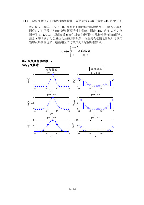
(1) 观察高斯序列的时域和幅频特性,固定信号)(n x a 中参数p=8,改变q 的值,使q 分别等于2、4、8,观察他们的时域和幅频特性,了解当q 取不同值时,对信号序列的时域和幅频特性的影响;固定q=8,改变p,使p 分别等于8、13、14,观察参数p 变化对信号序列的时域和幅频特性的影响,注意p 等于多少时会发生明显的泄漏现象,混叠是否也随之出现?记录实验中观察到的现象,绘出相应的时域序列和幅频特性曲线。
()()⎪⎩⎪⎨⎧≤≤=-其他0150,2n e n x q p n a解:程序见附录程序一:P=8,q 变化时:t/T x a (n )k X a (k )t/T x a (n )p=8 q=4k X a (k )p=8 q=4t/Tx a (n )p=8 q=8kX a (k )p=8 q=8幅频特性时域特性t/T x a (n )p=8 q=8k X a (k )p=8 q=8t/T x a (n )51015k X a (k )p=13 q=8t/Tx a (n )p=14 q=851015kX a (k )p=14 q=8时域特性幅频特性分析:由高斯序列表达式知n=p 为期对称轴; 当p 取固定值时,时域图都关于n=8对称截取长度为周期的整数倍,没有发生明显的泄漏现象;但存在混叠,当q 由2增加至8过程中,时域图形变化越来越平缓,中间包络越来越大,可能函数周期开始增加,频率降低,渐渐小于fs/2,混叠减弱;当q 值固定不变,p 变化时,时域对称中轴右移,截取的时域长度渐渐地不再是周期的整数倍,开始无法代表一个周期,泄漏现象也来越明显,因而图形越来越偏离真实值,p=14时的泄漏现象最为明显,混叠可能也随之出现;(2) 观察衰减正弦序列 的时域和幅频特性,a=0.1,f=0.0625,检查谱峰出现的位置是否正确,注意频谱的形状,绘出幅频特性曲线,改变f ,使f 分别等于0.4375和0.5625,观察这两种情况下,频谱的形状和谱峰出现的位置,有无混叠和泄漏现象?说明产生现象的原因。
(完整版)数字信号处理实验二

y = filter(num,den,x,ic);
yt = a*y1 + b*y2;
d = y - yt;
subplot(3,1,1)
stem(n,y);
ylabel('振幅');
title('加权输入: a \cdot x_{1}[n] + b \cdot x_{2}[n]的输出');
subplot(3,1,2)
%扫频信号通过2.1系统:
clf;
n = 0:100;
s1 = cos(2*pi*0.05*n);
s2 = cos(2*pi*0.47*n);
a = pi/2/100;
b = 0;
arg = a*n.*n + b*n;
x = cos(arg);
M = input('滤波器所需的长度=');
num = ones(1,M);
三、实验器材及软件
1.微型计算机1台
2. MATLAB 7.0软件
四、实验原理
1.三点平滑滤波器是一个线性时不变的有限冲激响应系统,将输出延时一个抽样周期,可得到三点平滑滤波器的因果表达式,生成的滤波器表示为
归纳上式可得
此式表示了一个因果M点平滑FIR滤波器。
2.对线性离散时间系统,若y1[n]和y2[n]分别是输入序列x1[n]和x2[n]的响应,则输入
plot(n, y);
axis([0, 100, -2, 2]);
xlabel('时间序号 n'); ylabel('振幅');
数字信号处理习题答案及matlab实验详解.pdf
阶跃响应为: y[n] x[n] h[n] x[m]h[n m] h(n m), n m, m 0
m
m0
即 y(0) 0, y(1) 0.25, y(2) 0.5, y(3) 0.75,其余y(n) 1, (n 3)
利用函数 h=impz(b,a,N)和 y=filter(b,a,x)分别绘出冲激和阶跃响应 b=[0,0.25,0.25,0.25,0.25]; a=1; x=ones(1,100); h=impz(b,a,100);y=filter(b,a,x) figure(1) subplot(2,1,1); stem(h,’.’); subplot(2,1,2); plot(y,’.’);
4
解:(1)系统的转移函数是是其单位抽样响应的 Z 变换,因此
H (z)
1 1 z1
1 1 0.3z1
1 1 0.6z1
(1
3 3.8z1 1.08z2 z1)(1 0.3z1)(1 0.6z1)
1
3 1.9
3.8z1 1.08z2 z1 1.08z2 0.18z
3
Z 1
系统的零极点图如下图所示: B=[3,-3.8,1.08]; A=[1,-1.9,1.08,-0.18]; [Z,P,K]=tf2zp(B,A); Zplane(B,A)
5
单位抽样响应:
h(n)
1 2
n1
u
(n
1)
(n)
1
y(n) x(n) * h(n)
2 m1
1 2
m1
e
j (n m)
e
jn
e
jn
e j
1 2 1
2
n
u(n1)
数字信号处理 课后习题答案 第2章.docx

习题1.设X(e"。
)和r(e JC0)分别是印7)和)仞的傅里叶变换,试求下面序列的傅里叶变换:(1) x("-"o) (3) x(-n) (5) x(")y(")(7) x(2n)⑵ x*(〃)(4) x(") * v(«) (6) nx(n) (8) /(〃)解:⑴00 FT[X(/7-Z70)] = £x(〃一〃o)e—S令n r = n-n0,即〃=n' + n Q,贝!J00FT[x(n-n o y\=工》(〃')以"''*""="初。
乂(烈)00 00(2)FT[x («)] = £ x* (n)e*= [ £ 戏〃)攻以]* = X* (e「W=—00 w=—00(3)00FT[x(—")]= 〃)e*"令=一〃,则00FT[x(—”)]= Zx(〃')e" =X(e—〃")”'=—00(4)00 x(〃) *'(〃)= ^\x(jrT)y(n -m)W=-0000 00FT[x(n) * v(w)] = Z【Z x("y("-初)]e""' n=-<x> w=-oo k = n-m,贝U00 00FT[x(ri)*y(ri)]= £[ £x(初) k=—CD W=-0000 00k=-<x> m=—cc= X(e5(em)_00 00 1时[x(M)贝〃)]= Z》(〃)贝〃)e「9 = Zx(〃)[-Lf/(em'"'"d 渺]e-加""=—00 〃=—00 2l "1 00=—£ Y(e j0)')2l " n=—<x>1 伙=一L "口")*?®"、技或者FT[x{n)y{ny\ = —「171 »兀oo(6)因为X(e,")= »("初,对该式两边口求导,得到叫、)=-J £仗"如=-jFT[nx(n)]因此矶孙(〃)]=j至@3)dco00⑺ FT\x(2ri)\=加n=-(x)令n' = 2n ,则FT[X(2W)]= £x(z/)e 7 %W--00,且取偶数00 1 r r・l 八1°0 . 1 00 . 1£?kO + (T)“x(")厂=| 广伽+£ef ("广伽〃=—oo 匕匕〃=—oo 〃=—00=L「xa*+x(/*E)F7[x(2z?)] = | X(e‘2") + X(—e'尸)(8) F7[X2(»)]= J X2(77)6^»=-OO利用(5)题结果,令x{n) = y{n),则F巾2(”)] = _£x(em)*X(eS) = —「X®。
数字信号处理实验(吴镇扬)答案-2

(1) 观察高斯序列的时域和幅频特性,固定信号)(n x a 中参数p=8,改变q 的值,使q 分别等于2、4、8,观察他们的时域和幅频特性,了解当q 取不同值时,对信号序列的时域和幅频特性的影响;固定q=8,改变p,使p 分别等于8、13、14,观察参数p 变化对信号序列的时域和幅频特性的影响,注意p 等于多少时会发生明显的泄漏现象,混叠是否也随之出现?记录实验中观察到的现象,绘出相应的时域序列和幅频特性曲线。
()()⎪⎩⎪⎨⎧≤≤=-其他0150,2n e n x q p n a解:程序见附录程序一:P=8,q 变化时:t/T x a (n )p=8 q=2k X a (k )t/T x a (n )p=8 q=4k X a (k )p=8 q=4t/Tx a (n )p=8 q=8kX a (k )p=8 q=8幅频特性时域特性t/T x a (n )p=8 q=8k X a (k )p=8 q=8t/T x a (n )p=13 q=851015k X a (k )p=13 q=8t/Tx a (n )p=14 q=851015kX a (k )p=14 q=8时域特性幅频特性分析:由高斯序列表达式知n=p 为期对称轴; 当p 取固定值时,时域图都关于n=8对称截取长度为周期的整数倍,没有发生明显的泄漏现象;但存在混叠,当q 由2增加至8过程中,时域图形变化越来越平缓,中间包络越来越大,可能函数周期开始增加,频率降低,渐渐小于fs/2,混叠减弱;当q 值固定不变,p 变化时,时域对称中轴右移,截取的时域长度渐渐地不再是周期的整数倍,开始无法代表一个周期,泄漏现象也来越明显,因而图形越来越偏离真实值,p=14时的泄漏现象最为明显,混叠可能也随之出现;(2) 观察衰减正弦序列 的时域和幅频特性,a=0.1,f=0.0625,检查谱峰出现的位置是否正确,注意频谱的形状,绘出幅频特性曲线,改变f ,使f 分别等于0.4375和0.5625,观察这两种情况下,频谱的形状和谱峰出现的位置,有无混叠和泄漏现象?说明产生现象的原因。
数字信号处理 刘顺兰第二章完整版习题解答
即 0 不在采样点上时,
X (k )
1 e
1 e
b 当 ○
j ( 0
1 e 1 e
j 0 N 2 k) N
j ( 0
sin[(
0
2
N
k)N ] e ) N
j(
0
2 N
k )( N 1)
sin(
0
2
k
0
X (1) 2 2 j
nk N
x(n)W
n 0
N 1
k 2k 3k 1 jW N WN jW N ,
可求得 X (0) 0,
N 1 n 0
X (1) 4, X (2) 0 , N ( k ) c 1 N 1 c c 1 k cW N
(3) x( n) c , 0 n N 1
n
解: (1) X ( k )
x(n)W
n 0
3
nk 4
1 W4k W42 k W43k , k 0,1,2,3 X (2) 0, X (3) 2 2 j N 4
可求得 X (0) 0, (2) X ( k )
1 N 1 j ( k ' k ) n N 1 j N ( k k ') n X ( k ) [ e N e ] 2 n 0 n 0 N , 2 0 ,
(3) X ( k )
N 1 N 1 n 0
2
2
k k ' 及k N k ' 其它
k N
1 k N 1
即
N ( N 1) , 2 X (k ) N k , W N 1
数字信号处理米特拉第四版实验二答案

Name: SOLUTIONSection:Laboratory Exercise 2DISCRETE-TIME SYSTEMS: TIME-DOMAIN REPRESENTATION 2.1 SIMULATION OF DISCRETE-TIME SYSTEMSProject 2.1The Moving Average SystemA copy of Program P2_1 is given below:% Program P2_1% Simulation of an M-point Moving Average Filter% Generate the input signaln = 0:100;s1 = cos(2*pi*0.05*n); % A low-frequency sinusoids2 = cos(2*pi*0.47*n); % A high frequency sinusoidx = s1+s2;% Implementation of the moving average filterM = input('Desired length of the filter = ');num = ones(1,M);y = filter(num,1,x)/M;% Display the input and output signalsclf;subplot(2,2,1);plot(n, s1);axis([0, 100, -2, 2]);xlabel('Time index n'); ylabel('Amplitude');title('Signal #1');subplot(2,2,2);plot(n, s2);axis([0, 100, -2, 2]);xlabel('Time index n'); ylabel('Amplitude');title('Signal #2');subplot(2,2,3);plot(n, x);axis([0, 100, -2, 2]);xlabel('Time index n'); ylabel('Amplitude');title('Input Signal');subplot(2,2,4);plot(n, y);axis([0, 100, -2, 2]);xlabel('Time index n'); ylabel('Amplitude');title('Output Signal');axis;Answers:Q2.1 The output sequence generated by running the above program for M = 2 with x[n] =s1[n]+s2[n] as the input is shown below .50100-2-1012Time index n A m p l i t u d eSignal #150100-2-1012Time index n A m p l i t u d eSignal #250100-2-1012Time index nA m p l i t u d eInput Signal50100-2-1012Time index nA m p l i t u d eOutput SignalThe component of the input x[n] suppressed by the discrete-time system simulated by this program is – Signal #2, the high frequency one (it is a low pass filter).Q2.2Program P2_1 is modified to simulate the LTI system y[n] = 0.5(x[n]–x[n–1]) and process the input x[n] = s1[n]+s2[n] resulting in the output sequence shown below :Note: the code is not required; however, it is included here to demonstrate a tricky way ofmaking the modification to P2_1.% Program Q2_2% Modification of P1_1 to convert it to a high pass filter % Generate the input signal n = 0:100;s1 = cos(2*pi*0.05*n); % A low-frequency sinusoid s2 = cos(2*pi*0.47*n); % A high frequency sinusoid x = s1+s2;% Implementation of high pass filterM = input('Desired length of the filter = ');% By comparing eq. (2.13) to (2.3), you can see that "num" % actually contains the impulse response (times the constant % M). What we are actually doing in Q2.2 is multiplying the % impulse response of the low pass filter in P2_1 by the % sequency (-1)^n. This shifts the low pass frequency% response up to be centered at f=0.25, making it a high % pass filter.num = (-1).^[0:M-1]; y = filter(num,1,x)/M;% Display the input and output signals clf;subplot(2,2,1); plot(n, s1);axis([0, 100, -2, 2]);xlabel('Time index n'); ylabel('Amplitude'); title('Signal #1'); subplot(2,2,2); plot(n, s2);axis([0, 100, -2, 2]);xlabel('Time index n'); ylabel('Amplitude'); title('Signal #2'); subplot(2,2,3); plot(n, x);axis([0, 100, -2, 2]);xlabel('Time index n'); ylabel('Amplitude'); title('Input Signal'); subplot(2,2,4); plot(n, y);axis([0, 100, -2, 2]);xlabel('Time index n'); ylabel('Amplitude'); title('Output Signal'); axis;Time index n A m p l i t u d eSignal #1-2-1012Time index n A m p l i t u d eSignal #2Time index nA m p l i t u d eInput Signal-2-1012Time index nA m p l i t u d eOutput SignalThe effect of changing the LTI system on the input is – The system is now a high pass filter.It passes the high-frequency input component s2 instead of the low frequency input component s1.Q2.3Program P2_1 is run for the following values of filter length M and following values of the fre-quencies of the sinusoidal signals s1[n] and s2[n]. The output generated for these different values of M and the frequencies are shown below.f1=0.05; f2=0.47; M=1550100-2-1012Time index n A m p l i t u d eSignal #150100Time index n A m p l i t u d eSignal #250100-2-1012Time index nA m p l i t u d eInput Signal50100Time index nA m p l i t u d eOutput SignalFrom these plots we make the following observations – with M=15, the low passcharacteristic is much more pronounced (the passband is now very narrow). s2 is still nearly eliminated in the output signal. s1 is still passed, but at an attenuated level.f1=0.30; f2=0.47; M=4-2-1012Time index n A m p l i t u d eSignal #1Time index n A m p l i t u d eSignal #2-2-1012Time index nA m p l i t u d eInput SignalTime index nA m p l i t u d eOutput SignalFrom these plots we make the following observations – with M=4, this filter performs moresmoothing than in the case M=2. Both s1 and s2 are high frequency in this case, and they are both substantially attenuated in the output.f1=0.05; f2=0.10; M=3-2-1012Time index n A m p l i t u d eSignal #1Time index n A m p l i t u d eSignal #2-2-1012Time index nA m p l i t u d eInput SignalTime index nA m p l i t u d eOutput SignalFrom these plots we make the following observations – here s1 and s2 are both low passand they are both visible in the filter output. However, s2, the higher frequency input,is attenuated slightly more than s1 in the system output.Q2.4 The required modifications to Program P2_1 by changing the input sequence to a swept-frequency sinusoidal signal (length 101, minimum frequency 0, and a maximum frequency 0.5) as the input signal (see Program P1_7) are listed below:% Program Q2_4% Modify P2_1 to use a swept frequency chirp input% Generate the input signaln = 0:100;a = pi/200;b = 0;arg = a*n.*n + b*n;x = cos(arg);% Implementation of the moving average filterM = input('Desired length of the filter = ');num = ones(1,M);y = filter(num,1,x)/M;% Display the input and output signalsclf;subplot(2,1,1);plot(n, x);axis([0, 100, -1.5, 1.5]);xlabel('Time index n'); ylabel('Amplitude');title('Input Signal');subplot(2,1,2);plot(n, y);axis([0, 100, -1.5, 1.5]);xlabel('Time index n'); ylabel('Amplitude');title('Output Signal');axis;The output signal generated by running this program is plotted below .102030405060708090100-101Time index n A m p l i t u d eInput Signal102030405060708090100-101Time index nA m p l i t u d eOutput SignalThe results of Questions Q2.1 and Q2.2 from the response of this system to the swept-frequency signal can be explained as follows : we see again that this system is a low passfilter. At the left of the graphs, the input signal is a low frequency sinusoid that is passed to the output without attenuation. As n increases, the frequency of the input rises, and increasing attenuation is seen at the output. In Q2.1, the input was a sum of two sinusoids s1 and s2 with f1=0.05 and f2=0.47. The swept frequency input of Q2.4 reaches a frequency of 0.05 at n=10, where there is virtually no attenuation in the output shown above. This “explains” why s1 was passed by the system in Q2.1. The swept frequency input of Q2.4 reaches a frequency of 0.47 at approximately n=94, where the attenuation of the system is substantial. This “explains” why s2 was almost completely suppressed in the output in Q2.1.There is no direct relationship between the result shown above for Q2.4 and the result obtained in Q2.2. However, using frequency domain concepts (Chapter 3) we can reason that, if the swept frequency signal was input to the system y[n] = 0.5(x[n] – x[n-1]), we would see a result opposite to what is shown above. Since the system would then be a high pass filter, there would be substantial attenuation of the output at the left side of the graph and virtually no attenuation at the right side of the graph. This “explains” why in Q2.2 the low frequency component s1 was suppressed in the system output, whereas the high frequency component s2 was passed.Project 2.2 (Optional) A Simple Nonlinear Discrete-Time SystemA copy of Program P2_2 is given below:% Program P2_2% Generate a sinusoidal input signalclf;n = 0:200;x = cos(2*pi*0.05*n);% Compute the output signalx1 = [x 0 0]; % x1[n] = x[n+1]x2 = [0 x 0]; % x2[n] = x[n]x3 = [0 0 x]; % x3[n] = x[n-1]y = x2.*x2-x1.*x3;y = y(2:202);% Plot the input and output signalssubplot(2,1,1)plot(n, x)xlabel('Time index n');ylabel('Amplitude');title('Input Signal')subplot(2,1,2)plot(n,y)xlabel('Time index n');ylabel('Amplitude');title('Output signal');Answers:Q2.5The sinusoidal signals with the following frequencies as the input signals were used to generate the output signals: f=0.05, f=0.1, f=0.25The output signals generated for each of the above input signals are displayed below:Time index nA m p l i t u d eTime index nA m p l i t u d eOutput SignalTime index nA m p l i t u d eThe output signals depend on the frequencies of the input signal according to the following rules : up to “edge effects” visible at the very left and right sides of the first graph, theoutput is given by y[n] = sin 2(2πf).This observation can be explained mathematically as follows : Let 2f ω=π. Then[]cos()x n n =ω and22[]cos ()x n n =ω (1.1)Now, [1]cos[(1)]cos()x n n n +=ω+=ω+ω and [1]cos[(1)]x n n −=ω−= cos()n ω−ω, so [1][1]cos()cos()x n x n n n +−=ω+ωω−ω. Applying the trigonometric identity 1122cos()cos()cos(2)cos(2)A B A B A B +−=+, this becomes11[1][1]cos(2)cos(2).22x n x n n +−=ω+ω (1.2) Applying the trigonometric identity 2cos(2)2cos ()1A A =− to the first term of (1.2), we obtain211[1][1]cos ()cos(2).22x n x n n +−=ω−+ω (1.3)Applying the identity 2cos(2)12sin ()A A =−to the second term of (1.3) gives us22[1][1]cos ()sin ().x n x n n +−=ω−ω (1.4)It follows immediately from (1.1) and (1.4) that222[][][1][1]sin ()sin (2).y n x n x n x n f =−+−=ω=πQ2.6The output signal generated by using sinusoidal signals of the form x[n] = sin(ωo n) +K as the input signal is shown below for the following values of ωo and K -ωo = 0.1; K = 0.5Time index nA m p l i t u d eOutput SignalThe dependence of the output signal y[n] on the DC value K can be explained as –Again let2.f ω=π Then []cos()x n n K =ω+ and222[]cos ()2cos().x n n K n K =ω+ω+ (1.5)We have [1]cos[(1)]cos()x n n K n K +=ω++=ω+ω+and[1]cos[(1)]cos().x n n K n K −=ω−+=ω−ω+ So2[1][1]cos()cos()cos()cos().x n x n n n K n K n K +−=ω+ωω−ω+ω+ω+ω−ω+(1.6)From (1.4), we have that 22cos()cos()cos ()sin (),n n n n ω+ωω−ω=ω−ωso (1.6) may be written as222[1][1]cos ()sin ()[cos()cos()].x n x n n n K n n K +−=ω−ω+ω+ω+ω−ω+(1.7)Applying the trigonometric identity cos()cos()2cos()cos()A B A B A B ++−=to the term in square brackets in (1.7), we have that22[1][1]cos ()sin ()2cos()cos()2.x n x n K n K +−=ω−ω+ωω+Combining the this result with (1.5), it follows immediately that2[]sin (2)2[1cos(2)]cos(2).y n f K f fn =π+−ππSo addition of the constant K to the input cosine signal has the effect of adding a ripple onto the result that was obtained before in Q2.5. This ripple is a cosine wave of frequency f and amplitude 2[1cos(2)],K f −πas can be seen plainly in the graph above.Project 2.3Linear and Nonlinear SystemsA copy of Program P2_3 is given below :% Program P2_3% Generate the input sequences clf;n = 0:40; a = 2;b = -3;x1 = cos(2*pi*0.1*n); x2 = cos(2*pi*0.4*n); x = a*x1 + b*x2;num = [2.2403 2.4908 2.2403]; den = [1 -0.4 0.75];ic = [0 0]; % Set zero initial conditionsy1 = filter(num,den,x1,ic); % Compute the output y1[n] y2 = filter(num,den,x2,ic); % Compute the output y2[n] y = filter(num,den,x,ic); % Compute the output y[n] yt = a*y1 + b*y2;d = y - yt; % Compute the difference output d[n] % Plot the outputs and the difference signal subplot(3,1,1) stem(n,y);ylabel('Amplitude');title('Output Due to Weighted Input: a \cdot x_{1}[n] + b \cdot x_{2}[n]'); subplot(3,1,2) stem(n,yt);ylabel('Amplitude');title('Weighted Output: a \cdot y_{1}[n] + b \cdot y_{2}[n]'); subplot(3,1,3) stem(n,d);xlabel('Time index n');ylabel('Amplitude'); title('Difference Signal');Answers: Q2.7The outputs y[n], obtained with weighted input, and yt[n], obtained by combining the two outputs y1[n] and y2[n] with the same weights, are shown below along with the difference between the two signals :0510152025303540A m p l i t u d eOutput Due to Weighted Input: a ⋅ x 1[n] + b ⋅ x 2[n]0510152025303540A m p l i t u d eWeighted Output: a ⋅ y 1[n] + b ⋅ y 2[n]x 10-15Time index nA m p l i t u d eDifference SignalThe two sequences are – the same up to numerical roundoff. The system is – Linear.Q2.8 Program P2_3 was run for the following three different sets of values of the weightingconstants, a and b , and the following three different sets of input frequencies :1. a=1; b=-1; f1=0.05; f2=0.4;2. a=10; b=2; f1=0.10; f2=0.25;3. a=2; b=10; f1=0.15; f2=0.20;The plots generated for each of the above three cases are shown below :0510152025303540A m p l i t u d eOutput Due to Weighted Input: a ⋅ x 1[n] + b ⋅ x 2[n]0510152025303540A m p l i t u d eWeighted Output: a ⋅ y 1[n] + b ⋅ y 2[n]0510152025303540x 10-15Time index nA m p l i t u d eDifference Signal0510152025303540A m p l i t u d eOutput Due to Weighted Input: a ⋅ x 1[n] + b ⋅ x 2[n]0510152025303540A m p l i t u d eWeighted Output: a ⋅ y 1[n] + b ⋅ y 2[n]0510152025303540x 10-14Time index nA m p l i t u d eDifference SignalA m p l i t u d eOutput Due to Weighted Input: a ⋅ x 1[n] + b ⋅ x 2[n]0510152025303540A m p l i t u d eWeighted Output: a ⋅ y 1[n] + b ⋅ y 2[n]0510152025303540x 10-14Time index nA m p l i t u d eDifference SignalBased on these plots we can conclude that the system with different weights is – Linear.Q2.9 Program 2_3 was run with the following non-zero initial conditions – ic = [5 10];The plots generated are shown below -A m p l i t u d eOutput Due to Weighted Input: a ⋅ x 1[n] + b ⋅ x 2[n]A m p l i t u d eWeighted Output: a ⋅ y 1[n] + b ⋅ y 2[n]Time index nA m p l i t u d eDifference SignalBased on these plots we can conclude that the system with nonzero initial conditions is –Nonlinear.Q2.10Program P2_3 was run with nonzero initial conditions and for the following three different sets of values of the weighting constants, a and b , and the following three different sets of input frequencies :1. a=1; b=-1; f1=0.05; f2=0.4;2. a=10; b=2; f1=0.10; f2=0.25;3. a=2; b=10; f1=0.15; f2=0.20;The plots generated for each of the above three cases are shown below :0510152025303540A m p l i t u d eOutput Due to Weighted Input: a ⋅ x 1[n] + b ⋅ x 2[n]0510152025303540A m p l i t u d eWeighted Output: a ⋅ y 1[n] + b ⋅ y 2[n]0510152025303540Time index nA m p l i t u d eDifference Signal0510152025303540A m p l i t u d eOutput Due to Weighted Input: a ⋅ x 1[n] + b ⋅ x 2[n]0510152025303540A m p l i t u d eWeighted Output: a ⋅ y 1[n] + b ⋅ y 2[n]0510152025303540Time index nA m p l i t u d eDifference Signal0510152025303540A m p l i t u d eOutput Due to Weighted Input: a ⋅ x 1[n] + b ⋅ x 2[n]0510152025303540A m p l i t u d eWeighted Output: a ⋅ y 1[n] + b ⋅ y 2[n]0510152025303540Time index nA m p l i t u d eDifference SignalBased on these plots we can conclude that the system with nonzero initial conditions and different weights is – Nonlinear.Q2.11 Program P2_3 was modified to simulate the system :y[n] = x[n]x[n –1]The output sequences y1[n], y2[n],and y[n]of the above system generated by running the modified program are shown below :0510152025303540y 1[n]0510152025303540y 2[n]y t [n]0510152025303540A m p l i t u d eOutput Due to Weighted Input: a ⋅ x 1[n] + b ⋅ x 2[n]0510152025303540A m p l i t u d eWeighted Output: a ⋅ y 1[n] + b ⋅ y 2[n]0510152025303540Time index nA m p l i t u d eDifference SignalComparing y[n] with yt[n] we conclude that the two sequences are – Not the Same. This system is – Nonlinear.Project 2.4 Time-invariant and Time-varying SystemsA copy of Program P2_4 is given below:% Program P2_4% Generate the input sequencesclf;n = 0:40; D = 10;a = 3.0;b = -2;x = a*cos(2*pi*0.1*n) + b*cos(2*pi*0.4*n);xd = [zeros(1,D) x];num = [2.2403 2.4908 2.2403];den = [1 -0.4 0.75];ic = [0 0]; % Set initial conditions% Compute the output y[n]y = filter(num,den,x,ic);% Compute the output yd[n]yd = filter(num,den,xd,ic);% Compute the difference output d[n]d = y - yd(1+D:41+D);% Plot the outputssubplot(3,1,1)stem(n,y);ylabel('Amplitude');title('Output y[n]'); grid;subplot(3,1,2)stem(n,yd(1:41));ylabel('Amplitude');title(['Output due to Delayed Input x[n Ð', num2str(D),']']); grid; subplot(3,1,3)stem(n,d);xlabel('Time index n'); ylabel('Amplitude');title('Difference Signal'); grid;Answers: Q2.12The output sequences y[n] and yd[n] generated by running Program P2_4 are shown below -0510152025303540A m p l i t u d eOutput y[n]0510152025303540A m p l i t u d eOutput due to Delayed Input x[n -10]Time index nA m p l i t u d eDifference SignalThese two sequences are related as follows – y[n-10] = yd[n].The system is – Time Invariant.Q2.13 The output sequences y[n] and yd[n] generated by running Program P2_4 for thefollowing values of the delay variable D – 2; 6; 8.are shown below -0510152025303540A m p l i t u d eOutput y[n]0510152025303540A m p l i t u d eOutput due to Delayed Input x[n -2]0510152025303540Time index nA m p l i t u d eDifference Signal510152025303540A m p l i t u d eOutput y[n]0510152025303540A m p l i t u d eOutput due to Delayed Input x[n -6]0510152025303540Time index nA m p l i t u d eDifference Signal0510152025303540A m p l i t u d eOutput y[n]0510152025303540A m p l i t u d eOutput due to Delayed Input x[n -8]0510152025303540Time index nA m p l i t u d eDifference SignalIn each case, these two sequences are related as follows – y[n-D] = yd[n].The system is – Time Invariant.Q2.14 The output sequences y[n] and yd[n] generated by running Program P2_4 for thefollowing values of the input frequencies –1. f1=0.05; f2=0.40;2. f1=0.10; f2=0.25;3. f1=0.15; f2=0.20;are shown below –0510152025303540A m p l i t u d eOutput y[n]0510152025303540A m p l i t u d eOutput due to Delayed Input x[n -10]0510152025303540Time index nA m p l i t u d eDifference Signal510152025303540A m p l i t u d eOutput y[n]0510152025303540A m p l i t u d eOutput due to Delayed Input x[n -10]0510152025303540Time index nA m p l i t u d eDifference Signal0510152025303540A m p l i t u d eOutput y[n]0510152025303540A m p l i t u d eOutput due to Delayed Input x[n -10]0510152025303540Time index nA m p l i t u d eDifference SignalIn each case, these two sequences are related as follows – y[n-10] = yd[n].The system is – Time Invariant.Q2.15The output sequences y[n] and yd[n] generated by running Program P2_4 for non-zero initial conditions are shown below –0510152025303540A m p l i t u d eOutput y[n]0510152025303540A m p l i t u d eOutput due to Delayed Input x[n -10]0510152025303540Time index nA m p l i t u d eDifference SignalThese two sequences are related as follows – yd[n] is NOT equal to the shift of y[n].The system is – Time Varying.Q2.16The output sequences y[n] and yd[n] generated by running Program P2_4 for non-zero initial conditions and following values of the input frequencies –1. f1=0.05; f2=0.40;2. f1=0.10; f2=0.25;3. f1=0.15; f2=0.20;are shown below -0510152025303540A m p l i t u d eOutput y[n]A m p l i t u d eOutput due to Delayed Input x[n -10]0510152025303540Time index nA m p l i t u d eDifference Signal0510152025303540A m p l i t u d eOutput y[n]510152025303540A m p l i t u d eOutput due to Delayed Input x[n -10]0510152025303540Time index nA m p l i t u d eDifference SignalA m p l i t u d eOutput y[n]0510152025303540A m p l i t u d eOutput due to Delayed Input x[n -10]0510152025303540Time index nA m p l i t u d eDifference SignalIn each case, these two sequences are related as follows – yd[n] is NOT given by theshift of y[n].The system is – Time Varying.Q2.17The modified Program 2_4 simulating the systemy[n] = n x[n] + x[n-1]is given below :% Program Q2_17% Modification of P2_4 to implement the system% given by (2.16).% Generate the input sequencesclf;n = 0:40; D = 10;a = 3.0;b = -2;x = a*cos(2*pi*0.1*n) + b*cos(2*pi*0.4*n);xd = [zeros(1,D) x];nd = 0:length(xd)-1;% Compute the output y[n]y = (n .* x) + [0 x(1:40)];% Compute the output yd[n]yd = (nd .* xd) + [0 xd(1:length(xd)-1)];% Compute the difference output d[n]d = y - yd(1+D:41+D);% Plot the outputssubplot(3,1,1)stem(n,y);ylabel('Amplitude');title('Output y[n]'); grid;subplot(3,1,2)stem(n,yd(1:41));ylabel('Amplitude');title(['Output due to Delayed Input x[n -', num2str(D),']']); grid;subplot(3,1,3)stem(n,d);xlabel('Time index n'); ylabel('Amplitude');title('Difference Signal'); grid;The output sequences y[n]and yd[n] generated by running modified Program P2_4 are shown below -0510152025303540A m p l i t u d eOutput y[n]0510152025303540A m p l i t u d eOutput due to Delayed Input x[n -10]0510152025303540Time index nA m p l i t u d eDifference SignalThese two sequences are related as follows – yd[n] is NOT the shifted version of y[n]. The system is – Time Varying.Q2.18 (optional) The modified Program P2_3 to test the linearity of the system of (2.16) is shown below :% Program Q2_18% Modify P2_3 for Q2.18.% Generate the input sequences clf;n = 0:40; a = 2;b = -3;x1 = cos(2*pi*0.1*n); x2 = cos(2*pi*0.4*n); x = a*x1 + b*x2;y1 = (n .* x1) + [0 x1(1:40)]; % Compute the output y1[n] y2 = (n .* x2) + [0 x2(1:40)]; % Compute the output y2[n] y = (n .* x) + [0 x(1:40)]; % Compute the output y[n] yt = a*y1 + b*y2;d = y - yt; % Compute the difference output d[n] % Plot the outputs and the difference signal subplot(3,1,1) stem(n,y);ylabel('Amplitude');title('Output Due to Weighted Input: a \cdot x_{1}[n] + b \cdot x_{2}[n]'); subplot(3,1,2)stem(n,yt);ylabel('Amplitude');title('Weighted Output: a \cdot y_{1}[n] + b \cdot y_{2}[n]'); subplot(3,1,3) stem(n,d);xlabel('Time index n');ylabel('Amplitude'); title('Difference Signal');The outputs y[n]and yt[n] obtained by running the modified program P2_3 are shown below :0510152025303540A m p l i t u d eOutput Due to Weighted Input: a ⋅ x 1[n] + b ⋅ x 2[n]A m p l i t u d eWeighted Output: a ⋅ y 1[n] + b ⋅ y 2[n]0510152025303540x 10-14Time index nA m p l i t u d eDifference SignalThe two sequences are – The same up to numerical roundoff.The system is – Linear.2.5 LINEAR TIME-INVARIANT DISCRETE-TIME SYSTEMS Project 2.5Computation of Impulse Responses of LTI SystemsA copy of Program P2_5 is shown below :% Program P2_5% Compute the impulse response y clf; N = 40;num = [2.2403 2.4908 2.2403]; den = [1 -0.4 0.75]; y = impz(num,den,N);% Plot the impulse response stem(y);xlabel('Time index n'); ylabel('Amplitude'); title('Impulse Response'); grid;Answers:Q2.19 The first 41 samples of the impulse response of the discrete-time system of Project 2.3generated by running Program P2_5 is given below:-3-2-11234Time index nA m p l i t u d eImpulse ResponseQ2.20 The required modifications to Program P2_5 to generate the impulse response of the followingcausal LTI system :y[n] + 0.71y[n-1] – 0.46y[n-2] – 0.62y[n-3]= 0.9x[n] – 0.45x[n-1] + 0.35x[n-2] + 0.002x[n-3]are given below :% Program Q2_20% Compute the impulse response y clf; N = 45;num = [0.9 -0.45 0.35 0.002]; den = [1.0 0.71 -0.46 -0.62]; y = impz(num,den,N);% Plot the impulse response stem(y);xlabel('Time index n'); ylabel('Amplitude'); title('Impulse Response'); grid;The first 45 samples of the impulse response of this discrete-time system generated by running the modified is given below :051015202530354045-1.5-1-0.50.511.52Time index nA m p l i t u d eImpulse Responsethe filter command is indicated below :% Program Q2_21% Compute the impulse response y clf; N = 40;num = [0.9 -0.45 0.35 0.002]; den = [1.0 0.71 -0.46 -0.62]; % input: unit pulse x = [1 zeros(1,N-1)]; % outputy = filter(num,den,x);% Plot the impulse response% NOTE: the time axis will be WRONG; h[0] will % be plotted at n=1; but this will agree with % the INCORRECT plotting that was also done % by program P2_5. stem(y);xlabel('Time index n'); ylabel('Amplitude'); title('Impulse Response'); grid;The first 40 samples of the impulse response generated by this program are shown below :0510152025303540-1.5-1-0.50.511.52Time index nA m p l i t u d eImpulse ResponseComparing the above response with that obtained in Question Q2.20 we conclude - They are the SAME.indicated below :% Program Q2_22% Compute the step response s clf; N = 40; n = 0:N-1;num = [2.2403 2.4908 2.2403]; den = [1.0 -0.4 0.75]; % input: unit step x = [ones(1,N)]; % outputy = filter(num,den,x); % Plot the step response stem(n,y);xlabel('Time index n'); ylabel('Amplitude'); title('Step Response'); grid;The first 40 samples of the step response of the LTI system of Project 2.3 are shown below :0510152025303540Time index nA m p l i t u d eStep ResponseProject 2.6 Cascade of LTI SystemsA copy of Program P2_6 is given below:% Program P2_6% Cascade Realizationclf;x = [1 zeros(1,40)]; % Generate the inputn = 0:40;% Coefficients of 4th order systemden = [1 1.6 2.28 1.325 0.68];num = [0.06 -0.19 0.27 -0.26 0.12];% Compute the output of 4th order systemy = filter(num,den,x);% Coefficients of the two 2nd order systemsnum1 = [0.3 -0.2 0.4];den1 = [1 0.9 0.8];num2 = [0.2 -0.5 0.3];den2 = [1 0.7 0.85];% Output y1[n] of the first stage in the cascadey1 = filter(num1,den1,x);% Output y2[n] of the second stage in the cascadey2 = filter(num2,den2,y1);% Difference between y[n] and y2[n]d = y - y2;% Plot output and difference signalssubplot(3,1,1);stem(n,y);ylabel('Amplitude');title('Output of 4th order Realization'); grid;subplot(3,1,2);stem(n,y2)ylabel('Amplitude');title('Output of Cascade Realization'); grid;subplot(3,1,3);stem(n,d)xlabel('Time index n');ylabel('Amplitude');title('Difference Signal'); grid;Answers:Q2.23The output sequences y[n], y2[n], and the difference signal d[n]generated by running Program P2_6 are indicated below:。
数字信号处理(英文版)课后习题答案2
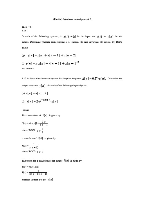
(Partial) Solutions to Assignment 2pp.73-761.16In each of the following systems, let or be the input and or be the output. Determine whether each systems is (1) linear, (2) time invariant, (3) causal, (4) BIBO stable(g).(i).ans: omitted----------------------------------------------------1.17 A linear time invariant system has impulse response Determine the output sequence for each of the followign input signals:(b)(f)(b) ans:h n is given byThe z-transform of []where ROC1:x n is given byz-transform of []where ROC2:h n is given byTherefore, the z-transform of the output []y nPerform inverse z to get [](f) ans: using the same method as in (b) (details omitted )----------------------------------------------------1.18. A linear time invariant system is defined by the difference equationb. Determine the output of the system when the intpu isc. Determine the output of the system when the input isans: omitted----------------------------------------------------1.19 The following expressions define linear time invariant systems. For each one determine the impulse respnose(a)(e)(a) ans: the impulse response is(e) ans: the impulse response is----------------------------------------------------1.20 Each of the following expressions defines a linear time invariant system. For each one determine whether it is BIBO stable or not(g)(k)BIBO: Bounded input and bounded output(g) ans: omitted(k) ans: omitted----------------------------------------------------1.21. Using the geometric series, for each of the following sequence determine the z-transform and its ROC(d)(g)(i)(d) ans:where ROC:(g) ans:The first part is equal towhere ROC1 isThe second part is equal towhere ROC2 isTherefore combining both parts:where ROC={ROC1 and ROC2}:(i) ans:where ROC: whole complex domain----------------------------------------------------1.22. You know what the and are. Using theproperties only (do not reuse the definition of the z-transform.) determine the z-transform of the following signals(c)(g)where ROC1:where ROC2:(c) ans: using z-transform property:We have:where ROC:(g) ans:details omitted. The final answer isTherefore combining both parts:where ROC={ROC1 and ROC2}:----------------------------------------------------1.23 Using partial fraction expansion, determine the inverse z-transform of the following functions:(c) ,(e) ,(c) ans:(e) ans:procedures are the same as above. details omitted.----------------------------------------------------1.24. For each of the followign linear difference equations, determine the impulse response, and indicate whether the system is BIBO stable or not(a)(c)(a) ans:Take z-transform on both sideswhere ROC:Because is finiteTherefore, the system is BIBO stable(c) ans: omitted (the same as (a))----------------------------------------------------1.25. Although most of the time we assume causality, a linear difference equation can be interpreted in a number of ways. Consider the linear difference equation(a) Determine the transfer function and the impulse response. Is the system causal ? BIBO stable ?(a) omitted.----------------------------------------------------1.26. 1.26 Consider the linear difference equation(a) Determine the transfer function . Do you have enough information to determine theregion of convergenceans:Don't have enough information to determine ROC.----------------------------------------------------1.27. Given the system described by the linear difference equationDetermine the output for each of the following input signals(a)(e)(a) ans:Take z-transform on both sides:----------------------------------------------------1.28. Repeat Problem 1.27 when the system is given in terms of the impulse responseBefore you do anything, is the system stable ? Does the frequency responseexist ?ans: omitted.----------------------------------------------------1.29. Repeat Problem 1.27 when the system isgiven by the linear difference equationBefore you do anything, is the system stable ? Does the frequency response exist ?Ans: omitted.----------------------------------------------------。
数字信号处理实验二
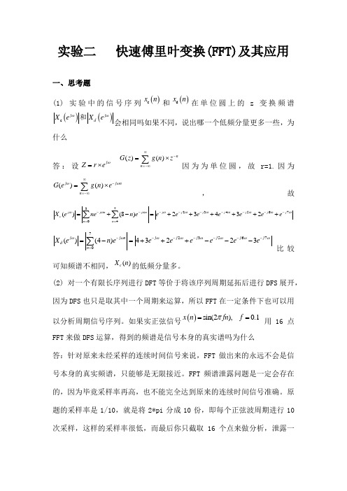
实验二 快速傅里叶变换(FFT)及其应用一、思考题(1) 实验中的信号序列()c x n 和()d x n 在单位圆上的z 变换频谱()()c j j d X e X e ωω和会相同吗如果不同,说出哪一个低频分量更多一些,为什么答:设j Z r e ω=⨯ ()()n n G z g n z ∞-=-∞=⨯∑因为为单位圆,故r=1.因为()()j j n n G e g n eωω∞-=-∞=⨯∑,故3723456704()(8)23432j j n j n j j j j j j j c n n X e nen e e e e e e e e ωωωωωωωωωω---------===+-=++++++∑∑ 7235670()(4)43223j j n j j j j j j d n X e n ee e e e e e ωωωωωωωω-------==-=+++---∑比较可知频谱不相同,()c X n 的低频分量多。
(2) 对一个有限长序列进行DFT 等价于将该序列周期延拓后进行DFS 展开,因为DFS 也只是取其中一个周期来运算,所以FFT 在一定条件下也可以用以分析周期信号序列。
如果实正弦信号()sin(2),0.1x n fn f π== 用16点FFT 来做DFS 运算,得到的频谱是信号本身的真实谱吗为什么答:针对原来未经采样的连续时间信号来说,FFT 做出来的永远不会是信号本身的真实频谱,只能够是无限接近。
FFT 频谱泄露问题是一定会存在的,因为毕竟采样率再高,也不能完全达到原来的连续时间信号准确。
原题的采样率是1/10,就是将2*pi 分成10份,即每个正弦波周期进行10次采样,这样的采样率很低,而最后你只截取16个点来做分析,泄露一般会挺严重,看到的频谱,应该是一个上头尖,下面慢慢变宽的尖锥形,而纯正的正弦波的理想频谱应该是在某频点只有一个尖峰。
二.?实验原理:?(1)混叠:采样序列的频谱是被采样信号频谱的周期延拓,当采样频率不满足奈奎斯特采样定理的时候,就会发生混叠,使得刺痒后的序列信号的频谱不能真实的反映原采样信号的频谱。
数字信号处理答案第2章

X (k ) − W X (k ) = ∑ WNkm − ( N − 1)
k N m =1
kn = ∑ W N − 1 − ( N − 1) = − N n =0 N −1
N −1
14
所以,
X (k ) =
−N , k ≠ 0 ,即 k 1 − WN N ( N − 1) k =0 2 X (k ) = −N k = 1, 2, L, N − 1 k 1 − WN
2. 已知下列X(k), 求x(n)=IDFT[X(k)]
N jθ 2e N − jθ X (k ) = e 2 0 k =m k = N −m 其它k
15
(1)
(2)
N jθ − j 2 e N − jθ X (k ) = j e 2 0
2π j( 2 π mn +θ ) − j( mn +θ ) 1 = e N +e N 2
2π = cos mn + θ N
n=0, 1, …, N-1
17
(2)
1 x ( n) = N
N jθ − mn N − jθ − ( N −m ) n − 2 je WN + 2 je WN
=
1− e
−j
2π (m−k ) N N 2π (m−k ) N
1− e
−j
N = 0
k =m k≠m
0≤k≤N-1
5
(6) X (k ) = ∑ cos
n =0
N −1
1 2π kn mn ⋅ WN = (e 2 N n =0
∑
N −1
j
2π mn N
数字信号处理实验指导书思考题答案实验图[精品文档]
![数字信号处理实验指导书思考题答案实验图[精品文档]](https://img.taocdn.com/s3/m/0d4c8b2b82c4bb4cf7ec4afe04a1b0717fd5b3aa.png)
数字信号处理实验指导书思考题答案实验图[精品⽂档]⽬录实验⼀ Matlab与数字信号处理基础 (2)实验⼆离散傅⾥叶变换与快速傅⾥叶变换 (4)实验三数字滤波器结构 (6)注释 (9)主要参考⽂献 (9)实验⼀ Matlab与数字信号处理基础⼀、实验⽬的和任务1、熟悉Matlab的操作环境2、学习⽤Matlab建⽴基本序列的⽅法;3、学习⽤仿真界⾯进⾏信号抽样的⽅法。
⼆、实验内容1、基本序列的产⽣:单位抽样序列、单位阶跃序列、矩形序列、实指数序列和复指数序列的产⽣2、⽤仿真界⾯进⾏信号抽样练习:⽤simulink建模仿真信号的抽样三、实验仪器、设备及材料计算机、Matlab软件四、实验原理序列的运算、抽样定理五、主要技术重点、难点Matlab的各种命令与函数、建模仿真抽样定理六、实验步骤1、基本序列的产⽣:单位抽样序列δ(n): n=-2:2;x=[0 0 1 0 0];stem(n,x);单位阶跃序列u(n):n=-10:10;x=[zeros(1,10) ones(1,11)];stem(n,x);矩形序列R N(n):n=-2:10;x=[0 0 ones(1,5) zeros(1,6)];stem(n,x);实指数序列0.5n:n=0:30;x=0.5.^nstem(n,x);复指数序列e(-0.2+j0. 3)n:n=0:30;x=exp((-0.2+j*0.3)*n);模:stem(n,abs(x));幅⾓:stem(n,angle(x));2、⽤仿真界⾯进⾏信号抽样练习:(1)在Matlab命令窗⼝中输⼊simulink 并回车,以打开仿真模块库;(2)按CTRL+N,以新建⼀仿真窗⼝;在仿真模块库中⽤⿏标点击Sources(输⼊源模块库),从中选择sine wave(正弦波模块)并将其拖⾄仿真窗⼝;(3)在仿真模块库中⽤⿏标点击Discrete(离散模块库),从中选择Zero-Order Hold(零阶保持器模块)并将其拖⾄仿真窗⼝;(4)在仿真模块库中⽤⿏标点击Sinks(显⽰模块库),从中选择Scope(⽰波器模块)并将其拖⾄仿真窗⼝;(5)在仿真窗⼝中把上述模块依次连接起来;(6)⽤⿏标双击Scope模块,以打开⽰波器的显⽰界⾯;(7)⽤⿏标点击仿真窗⼝⼯具条中的?图标开始仿真,结果显⽰在⽰波器中;(8)⽤⿏标双击Zero-Order Hold模块,打开其参数设置窗⼝,改变sample time参数值,例如1、0.5、0.1、0.05…,⽤⿏标点击仿真窗⼝⼯具条中的?图标开始仿真,⽐较⽰波器显⽰结果(选三个参数值,得三个结果);(9)在仿真模块库中⽤⿏标点击Sinks(显⽰模块库),从中选择To Workspace(输出到当前⼯作空间的变量模块)并将其拖⾄仿真窗⼝;(10)⽤⿏标双击To Workspace模块,打开其参数设置窗⼝,改变variable name参数值为x ;同时把save format参数值设置为Array ;(11)在仿真窗⼝中先⽤⿏标点击Zero-Order Hold模块与Scope模块的连线,然后按住CTRL 键,从选中连线的中部引出⼀条线到To Workspace模块;(12)⽤⿏标双击Zero-Order Hold模块,打开其参数设置窗⼝,改变sample time参数值,例如1、0.5、0.1、0.05…,⽤⿏标点击仿真窗⼝⼯具条中的?图标开始仿真,并返回命令窗⼝,⽤stem(x)作图,⽐较序列图显⽰结果(选三个参数值,得三个结果);七、实验报告要求1、实验步骤按实验内容指导进⾏;2、对于实验内容1和2的数据必须给出的离散图,其相关参数应在图中注明;3、具有关联性和⽐较性的图形最好⽤subplot()函数,把它们画在⼀起;4、实验报告按规定格式填写,要求如下:(1)实验步骤根据⾃⼰实际操作填写;(2)各⼩组实验数据不能完全相同,否则以缺席论处;5、实验结束,实验数据交指导教师检查,得到允许后可以离开,否则以缺席论处;⼋、实验注意事项1、Matlab编程、⽂件名、存盘⽬录均不能使⽤中⽂。
数字信号处理课后答案 第2章高西全
π
1 = 2π 1 = 2π
∫ ∫
π
−π
Y ( e jω ′ )
n = −∞
∑
x(n)e − j(ω −ω ′) n dω ′
π
−π
Y (e jω ′ ) X (e j(ω −ω ′) )dω ′
或者
1 FT[ x (n) y (n)] = 2π
(6) 因为
X ( e jω ) =
∫
π
−π
X (e jω ′ )Y (e j(ω −ω ′) )dω ′
m = −∞
∑
∞
x ( m ) e − j ωn
= x(e jω ) y (e jω )
(5)FT[ x(n) y (n)] =
n = −∞
∑
∞
∞
x ( n ) y ( n ) e − j ωn
1 x ( n) = 2π n = −∞
∑
∫
Y (e jω ′ )e jω ′n dω ′e − jωn −π
或者:
x3 (n) = u (n + 3) − u (n − 4) = R7 (n + 3)
X 4 ( e jω ) =
FT[ R7 (n)] =
n = −∞
∑
6 n =0
∞
R7 (n + 3)e − jωn
1 − e − j7ω = 1 − e − jω
∑
e − jωn
− j ωn
X 4 (e ) =
题4解图
或者
1 1 − j πk j πk e 2 (e 2 1 − j πk −e 2 )
~ X (k ) =
∑
n =0
1
数字信号处理实验二时域采样和频域采样
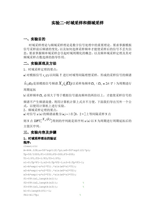
实验二-时域采样和频域采样一、实验目的时域采样理论与频域采样理论是数字信号处理中的重要理论。
要求掌握模拟信号采样前后频谱的变化,以及如何选择采样频率才能使采样后的信号不丢失信息;要求掌握频率域采样会引起时域周期化的概念,以及频率域采样定理及其对频域采样点数选择的指导作用。
二、实验原理及方法1、时域采样定理的要点:a)对模拟信号)(t x a 以间隔T 进行时域等间隔理想采样,形成的采样信号的频谱)(ˆΩj X 是原模拟信号频谱()aX j Ω以采样角频率s Ω(T s /2π=Ω)为周期进行周期延拓b)采样频率s Ω必须大于等于模拟信号最高频率的两倍以上,才能使采样信号的频谱不产生频谱混叠。
利用计算机计算上式并不方便,下面我们导出另外一个公式,以便用计算机上进行实验。
2、频域采样定理的要点:a)对信号x(n)的频谱函数X(ej ω)在[0,2π]上等间隔采样N 点 则N 点IDFT[()N X k ]得到的序列就是原序列x(n)以N 为周期进行周期延拓后的主值区序列。
三、实验内容及步骤1、时域采样理论的验证程序:clear;clcA=444.128;a=50*sqrt(2)*pi;w0=50*sqrt(2)*pi;Tp=50/1000;F1=1000;F2=300;F3=200;T1=1/F1;T2=1/F2;T3=1/F3;n1=0:Tp*F1-1;n2=0:Tp*F2-1;n3=0:Tp*F3-1;x1=A*exp(-a*n1*T1).*sin(w0*n1*T1);x2=A*exp(-a*n2*T2).*sin(w0*n2*T2);x3=A*exp(-a*n3*T3).*sin(w0*n3*T3);f1=fft(x1,length(n1));f2=fft(x2,length(n2)); %f3=fft(x3,length(n3)); %k1=0:length(f1)-1;fk1=k1/Tp; %k2=0:length(f2)-1;fk2=k2/Tp; % k3=0:length(f3)-1;fk3=k3/Tp; % subplot(3,2,1)stem(n1,x1,'.')title('(a)Fs=1000Hz');xlabel('n');ylabel('x1(n)');subplot(3,2,3)stem(n2,x2,'.')title('(b)Fs=300Hz');xlabel('n');ylabel('x2(n)');subplot(3,2,5)stem(n3,x3,'.')title('(c)Fs=200Hz');xlabel('n');ylabel('x3(n)');subplot(3,2,2)plot(fk1,abs(f1))title('(a) FT[xa(nT)],Fs=1000Hz'); xlabel('f(Hz)');ylabel('·ù¶È')subplot(3,2,4)plot(fk2,abs(f2))title('(b) FT[xa(nT)],Fs=300Hz'); xlabel('f(Hz)');ylabel('·ù¶È')subplot(3,2,6)plot(fk3,abs(f3))title('(c) FT[xa(nT)],Fs=200Hz'); xlabel('f(Hz)');ylabel('·ù¶È')结果分析:由图2.2可见,采样序列的频谱的确是以采样频率为周期对模拟信号频谱的周期延拓。
- 1、下载文档前请自行甄别文档内容的完整性,平台不提供额外的编辑、内容补充、找答案等附加服务。
- 2、"仅部分预览"的文档,不可在线预览部分如存在完整性等问题,可反馈申请退款(可完整预览的文档不适用该条件!)。
- 3、如文档侵犯您的权益,请联系客服反馈,我们会尽快为您处理(人工客服工作时间:9:00-18:30)。
实验二 离散时间信号的时域分析
1.实验目的
(1)学习MA TLAB 软件及其在信号处理中的应用,加深对常用离散时间信号的理解。
(2)利用MA TLAB 产生常见离散时间信号及其图形的显示,进行简单运算。
(3)熟悉MA TLAB 对离散信号的处理及其应用。
2.实验原理
离散时间信号是时间为离散变量的信号。
其函数值在时间上是不连续的“序列”。
(1)单位抽样序列
⎩⎨⎧=01
)(n δ 00≠=n n
如果序列在时间轴上面有K 个单位的延迟,则可以得到)(k n -δ,即:
1,()0,n k n k n k
d ì=ïï-=íï¹ïî 该序列可以用MA TLAB 中的zeros 函数来实现。
(2)正弦序列
)/2sin()(ϕπ+=Fs fn A n x
可以利用sin 函数来产生。
(3)指数序列
()(),n x n a n a R e =
在MA TLAB 中通过:0:1;n N =-和.^;x a n =来实现。
3.实验内容及其步骤
(1)复习有关离散时间信号的有关内容。
(2)通过程序实现上述几种信号的产生,并进行简单的运算操作。
① 单位抽样序列
⎩⎨⎧=01
)(n δ 00≠=n n
② 如果序列在时间轴上面有K 个单位的延迟,则可以得到)(k n -δ,即:
1,()0,n k n k n k
d ì=ïï-=íï¹ïî clf;
n = -10:20;
u = [zeros(1,10) 1 zeros(1,20)];
xlabel('Time index n');ylabel('Amplitude');
stem(n,u);
title('Unit Sample Sequence');
axis([-10 20 0 1.2]);
③ 正弦序列
)/2sin()(ϕπ+=Fs fn A n x
n = 0:40;
f = 0.1;
phase = 0;
A = 1.5;
arg = 2*pi*f*n - phase;
x = A*cos(arg);
clf;
stem(n,x);
axis([0 40 -2 2]);
grid;
title('Sinusoidal Sequence');
xlabel('Time index n');
ylabel('Amplitude');
axis;
④ 指数序列
()(),n x n a n a R e =
(3)加深对离散时间信号及其特性的理解,对于离散信号能进行基本的运算(例如信号加、乘、延迟等等),并且绘出其图形。
(4)通过实际的操作应用,实现对一段语音信号的简单处理。
4. 实验用MATLAB函数介绍
其中在实验过程中常用到的MATLAB指令(函数名)有:clf, zeros, ones, length, wavread, sound命令等,具体调用格式参看“help”或者查阅相关书籍。
另外,在具体的实验过程中也可以根据实际需要自己定义函数。
5.思考题
(1)离散时间信号在时域上有何特点。
(2)总结实验过程中所得到的结论,并能进行分析处理。
(3)对实验过程中所涉及的问题进行分析,对于信号经过时延之后,试编写和修改相应的程序,得出最终正确的结果和波形图,并对实验报告进行整理分析。
(4)对于离散时间信号进行计算。
6.实验报告要求:
(1)明确实验目的以及实验的原理。
(2)通过实验内容分析离散时间信号的性质。
(3)完成思考题的内容,对实验结果及其波形图进行分析对比,总结主要结论。
实验内容:
1.产生单位阶跃信号(用ones 函数)
2.产生指数序列 x(n)等于2乘以负一的n次方再乘以yisou n=-10:50;
k=sin(n);
u=2*(-1).^n.*k;
stem(n,u);
3.产生一个周期正弦函数
4.已知:x[n]={-4 5 1 -2 -3 0 2}, -4<n<4;
y[n]={6 -3 -1 0 8 7 -2}; -2<n<6;
编程计算x[n-1]和y[-n]的内积
5.求y[n]=a[n]*b[n] 用编程实现两个因果离散信号的卷积。