ansys公司培训教材疲劳分析
ansys疲劳分析基本方法
疲劳是指结构在低于静态极限强度载荷的重复载荷作用下,出现断裂破坏的现象。
例如一根能够承受 300 KN 拉力作用的钢杆,在 200 KN 循环载荷作用下,经历 1,000,000 次循环后亦会破坏。
导致疲劳破坏的主要因素如下:????? 载荷的循环次数;????? 每一个循环的应力幅;????? 每一个循环的平均应力;????? 存在局部应力集中现象。
????? 真正的疲劳计算要考虑所有这些因素,因为在预测其生命周期时,它计算“消耗”的某个部件是如何形成的。
???? ANSYS程序处理疲劳问题的过程????? ANSYS 疲劳计算以ASME锅炉和压力容器规范(ASME Boiler and Pressure Vessel Code)第三节(和第八节第二部分)作为计算的依据,采用简化了的弹塑性假设和Mimer累积疲劳准则。
????? 除了根据 ASME 规范所建立的规则进行疲劳计算外,用户也可编写自己的宏指令,或选用合适的第三方程序,利用 ANSYS 计算的结果进行疲劳计算。
《ANSYS APDL Programmer‘s Guide》讨论了上述二种功能。
????? ANSYS程序的疲劳计算能力如下:????? 对现有的应力结果进行后处理,以确定体单元或壳单元模型的疲劳寿命耗用系数(fatigue usage factors)(用于疲劳计算的线单元模型的应力必须人工输入);????? 可以在一系列预先选定的位置上,确定一定数目的事件及组成这些事件的载荷,然后把这些位置上的应力储存起来;????? 可以在每一个位置上定义应力集中系数和给每一个事件定义比例系数。
???? 基本术语?????位置(Location):在模型上储存疲劳应力的节点。
这些节点是结构上某些容易产生疲劳破坏的位置。
????? 事件(Event):是在特定的应力循环过程中,在不同时刻的一系列应力状态,见本章§。
????? 载荷(Loading):是事件的一部分,是其中一个应力状态。
ansys疲劳分析基本方法
疲劳是指结构在低于静态极限强度载荷的重复载荷作用下,出现断裂破坏的现象。
例如一根能够承受 300 KN 拉力作用的钢杆,在 200 KN 循环载荷作用下,经历 1,000,000 次循环后亦会破坏。
导致疲劳破坏的主要因素如下:载荷的循环次数;每一个循环的应力幅;每一个循环的平均应力;存在局部应力集中现象。
真正的疲劳计算要考虑所有这些因素,因为在预测其生命周期时,它计算“消耗”的某个部件是如何形成的。
3.1.1 ANSYS程序处理疲劳问题的过程ANSYS 疲劳计算以ASME锅炉和压力容器规(ASME Boiler and Pressure Vessel Code)第三节(和第八节第二部分)作为计算的依据,采用简化了的弹塑性假设和Mimer累积疲劳准则。
除了根据 ASME 规所建立的规则进行疲劳计算外,用户也可编写自己的宏指令,或选用合适的第三方程序,利用 ANSYS 计算的结果进行疲劳计算。
《ANSYS APDL Programmer‘s Guide》讨论了上述二种功能。
ANSYS程序的疲劳计算能力如下:对现有的应力结果进行后处理,以确定体单元或壳单元模型的疲劳寿命耗用系数(fatigue usage factors)(用于疲劳计算的线单元模型的应力必须人工输入);可以在一系列预先选定的位置上,确定一定数目的事件及组成这些事件的载荷,然后把这些位置上的应力储存起来;可以在每一个位置上定义应力集中系数和给每一个事件定义比例系数。
3.1.2 基本术语位置(Location):在模型上储存疲劳应力的节点。
这些节点是结构上某些容易产生疲劳破坏的位置。
事件(Event):是在特定的应力循环过程中,在不同时刻的一系列应力状态,见本章§3.2.3.4。
载荷(Loading):是事件的一部分,是其中一个应力状态。
应力幅:两个载荷之间应力状态之差的度量。
程序不考虑应力平均值对结果的影响。
3.2 疲劳计算完成了应力计算后,就可以在通用后处理器 POST1 中进行疲劳计算。
ansys疲劳分析解析

1.1 疲劳概述结构失效的一个常见原因是疲劳,其造成破坏与重复加载有关。
疲劳通常分为两类:高周疲劳是当载荷的循环(重复)次数高(如1e4 -1e9)的情况下产生的。
因此,应力通常比材料的极限强度低,应力疲劳(Stress-based)用于高周疲劳;低周疲劳是在循环次数相对较低时发生的。
塑性变形常常伴随低周疲劳,其阐明了短疲劳寿命。
一般认为应变疲劳(strain-based)应该用于低周疲劳计算。
在设计仿真中,疲劳模块拓展程序(Fatigue Module add-on)采用的是基于应力疲劳(stress-based)理论,它适用于高周疲劳。
接下来,我们将对基于应力疲劳理论的处理方法进行讨论。
1.2 恒定振幅载荷在前面曾提到,疲劳是由于重复加载引起:当最大和最小的应力水平恒定时,称为恒定振幅载荷,我们将针对这种最简单的形式,首先进行讨论。
否则,则称为变化振幅或非恒定振幅载荷。
1.3 成比例载荷载荷可以是比例载荷,也可以非比例载荷:比例载荷,是指主应力的比例是恒定的,并且主应力的削减不随时间变化,这实质意味着由于载荷的增加或反作用的造成的响应很容易得到计算。
相反,非比例载荷没有隐含各应力之间相互的关系,典型情况包括:σ1/σ2=constant在两个不同载荷工况间的交替变化;交变载荷叠加在静载荷上;非线性边界条件。
1.4 应力定义考虑在最大最小应力值σmin和σmax作用下的比例载荷、恒定振幅的情况:应力范围Δσ定义为(σmax-σmin)平均应力σm定义为(σmax+σmin)/2应力幅或交变应力σa是Δσ/2应力比R是σmin/σmax当施加的是大小相等且方向相反的载荷时,发生的是对称循环载荷。
这就是σm=0,R=-1的情况。
当施加载荷后又撤除该载荷,将发生脉动循环载荷。
这就是σm=σmax/2,R=0的情况。
1.5 应力-寿命曲线载荷与疲劳失效的关系,采用的是应力-寿命曲线或S-N曲线来表示:(1)若某一部件在承受循环载荷, 经过一定的循环次数后,该部件裂纹或破坏将会发展,而且有可能导致失效;(2)如果同个部件作用在更高的载荷下,导致失效的载荷循环次数将减少;(3)应力-寿命曲线或S-N曲线,展示出应力幅与失效循环次数的关系。
ansys疲劳分析基本方法
疲劳就是指结构在低于静态极限强度载荷的重复载荷作用下,出现断裂破坏的现象。
例如一根能够承受 300 KN 拉力作用的钢杆,在 200 KN 循环载荷作用下,经历 1,000,000 次循环后亦会破坏。
导致疲劳破坏的主要因素如下:载荷的循环次数;每一个循环的应力幅;每一个循环的平均应力;存在局部应力集中现象。
真正的疲劳计算要考虑所有这些因素,因为在预测其生命周期时,它计算“消耗”的某个部件就是如何形成的。
3、1、1 ANSYS程序处理疲劳问题的过程ANSYS 疲劳计算以ASME锅炉与压力容器规范(ASME Boiler and Pressure Vessel Code)第三节(与第八节第二部分)作为计算的依据,采用简化了的弹塑性假设与Mimer累积疲劳准则。
除了根据 ASME 规范所建立的规则进行疲劳计算外,用户也可编写自己的宏指令,或选用合适的第三方程序,利用 ANSYS 计算的结果进行疲劳计算。
《ANSYS APDL Programmer‘s Guide》讨论了上述二种功能。
ANSYS程序的疲劳计算能力如下:对现有的应力结果进行后处理,以确定体单元或壳单元模型的疲劳寿命耗用系数(fatigue usage factors)(用于疲劳计算的线单元模型的应力必须人工输入);可以在一系列预先选定的位置上,确定一定数目的事件及组成这些事件的载荷,然后把这些位置上的应力储存起来;可以在每一个位置上定义应力集中系数与给每一个事件定义比例系数。
3、1、2 基本术语位置(Location):在模型上储存疲劳应力的节点。
这些节点就是结构上某些容易产生疲劳破坏的位置。
事件(Event):就是在特定的应力循环过程中,在不同时刻的一系列应力状态,见本章§3、2、3、4。
载荷(Loading):就是事件的一部分,就是其中一个应力状态。
应力幅:两个载荷之间应力状态之差的度量。
程序不考虑应力平均值对结果的影响。
3、2 疲劳计算完成了应力计算后,就可以在通用后处理器 POST1 中进行疲劳计算。
ansys疲劳分析基本方法

疲劳是指结构在低于静态极限强度载荷的重复载荷作用下,出现断裂破坏的现象。
例如一根能够承受 300 KN 拉力作用的钢杆,在 200 KN 循环载荷作用下,经历 1,000,000 次循环后亦会破坏。
导致疲劳破坏的主要因素如下:载荷的循环次数;每一个循环的应力幅;每一个循环的平均应力;存在局部应力集中现象。
真正的疲劳计算要考虑所有这些因素,因为在预测其生命周期时,它计算“消耗”的某个部件是如何形成的。
3.1.1 ANSYS程序处理疲劳问题的过程ANSYS 疲劳计算以ASME锅炉和压力容器规范(ASME Boiler and Pressure Vessel Code)第三节(和第八节第二部分)作为计算的依据,采用简化了的弹塑性假设和Mimer累积疲劳准则。
除了根据 ASME 规范所建立的规则进行疲劳计算外,用户也可编写自己的宏指令,或选用合适的第三方程序,利用 ANSYS 计算的结果进行疲劳计算。
《ANSYS APDL Programmer‘s Guide》讨论了上述二种功能。
ANSYS程序的疲劳计算能力如下:对现有的应力结果进行后处理,以确定体单元或壳单元模型的疲劳寿命耗用系数(fatigue usage factors)(用于疲劳计算的线单元模型的应力必须人工输入);可以在一系列预先选定的位置上,确定一定数目的事件及组成这些事件的载荷,然后把这些位置上的应力储存起来;可以在每一个位置上定义应力集中系数和给每一个事件定义比例系数。
3.1.2 基本术语位置(Location):在模型上储存疲劳应力的节点。
这些节点是结构上某些容易产生疲劳破坏的位置。
事件(Event):是在特定的应力循环过程中,在不同时刻的一系列应力状态,见本章§3.2.3.4。
载荷(Loading):是事件的一部分,是其中一个应力状态。
应力幅:两个载荷之间应力状态之差的度量。
程序不考虑应力平均值对结果的影响。
3.2 疲劳计算完成了应力计算后,就可以在通用后处理器 POST1 中进行疲劳计算。
ansys公司培训教材疲劳分析

疲劳模块
本章概述
• • 本章将介绍疲劳模块拓展功能的使用:
– 使用者要先学习第4章线性静态结构分析.
培训手朋
ANSYS Workbench – Simulation ANSYS Workbench – Simulation ANSYS Workbench – Simulation ANSYS Workbench – Simulation
– 否则,则称为变化振幅或非恒定振幅 载荷 (本章之后将给予讨论).
February 20, 2004 Inventory #002018 14-4
疲劳模块
… 成比例载荷
•
培训手朋
ANSYS Workbench – Simulation ANSYS Workbench – Simulation ANSYS Workbench – Simulation ANSYS Workbench – Simulation
Availability x x x x x x
February 20, 2004 Inventory #002018 14-11
疲劳模块
… 疲劳程序
•
培训手朋
ANSYS Workbench – Simulation ANSYS Workbench – Simulation ANSYS Workbench – Simulation ANSYS Workbench – Simulation
… 恒定振幅载荷
• 在前面曾提到, 疲劳是由于重复加载 引起:
– 当最大和最小的应力水平恒定时, 称 为恒定振幅载荷. 我们将针对这种最 简单的形式,首先进行讨论.
培训手朋
ANSYS Workbench – Simulation ANSYS Workbench – Simulation ANSYS Workbench – Simulation ANSYS Workbench – Simulation
ANSYS疲劳分析

ANSYS疲劳分析疲劳是指结构在低于静态极限强度载荷的重复载荷作用下,出现断裂破坏的现象。
例如一根能够承受300 KN 拉力作用的钢杆,在200 KN 循环载荷作用下,经历1,000,000 次循环后亦会破坏。
导致疲劳破坏的主要因素如下:载荷的循环次数;每一个循环的应力幅;每一个循环的平均应力;存在局部应力集中现象。
真正的疲劳计算要考虑所有这些因素,因为在预测其生命周期时,它计算“消耗”的某个部件是如何形成的。
1.ANSYS程序处理疲劳问题的过程ANSYS 疲劳计算以ASME锅炉和压力容器规范(ASME Boiler and Pressure Vessel Code)作为计算的依据,采用简化了的弹塑性假设和Mimer累积疲劳准则。
除了根据ASME 规范所建立的规则进行疲劳计算外,用户也可编写自己的宏指令,或选用合适的第三方程序,利用ANSYS 计算的结果进行疲劳计算。
《ANSYS APDL Programmer’s Guide》讨论了上述二种功能。
ANSYS程序的疲劳计算能力如下:(1)对现有的应力结果进行后处理,以确定体单元或壳单元模型的疲劳寿命耗用系数(fatigue usage factors)(用于疲劳计算的线单元模型的应力必须人工输入);(2)可以在一系列预先选定的位置上,确定一定数目的事件及组成这些事件的载荷,然后把这些位置上的应力储存起来;(3)可以在每一个位置上定义应力集中系数和给每一个事件定义比例系数。
2.基本术语位置(Location):在模型上储存疲劳应力的节点。
这些节点是结构上某些容易产生疲劳破坏的位置。
事件(Event):是在特定的应力循环过程中,在不同时刻的一系列应力状态。
载荷(Loading):是事件的一部分,是其中一个应力状态。
应力幅:两个载荷之间应力状态之差的度量。
程序不考虑应力平均值对结果的影响。
3.疲劳计算完成了应力计算后,就可以在通用后处理器POST1 中进行疲劳计算。
疲劳分析1

ANSYS帮助中疲劳一章的翻译(1)(资料来源:半导体仿真论坛—)第13章疲劳13.1 疲劳的定义疲劳是结构在承受低于其极限载荷的力的反复作用下发生破裂的现象。
例如,一根钢条或许可以承受只有300KN的静态拉力的作用,但在200KN的力的反复作用下,就很可能发生破坏。
引起疲劳失效的主要因素包括:·经历的载荷周期数;·单周期内应力的变化幅度;·单周期内的平均应力;·局部应力集中的存在。
当计算在预计的生命周期中某个部分的耗用状况时,一个正式的疲劳评估要涉及以上任何一个因素。
13.1.1 ANSYS程序的任务ANSYS 疲劳计算是以ASME锅炉与压力容器规范的第3部分(和第8部分第二章)为依据,采用了简化了的弹塑性假设和Miner累积疲劳准则。
除了基于ASME规范的疲劳计算外,用户也可以自己定义宏指令,或者用合适的第三方程序与ANSYS分析结果相接。
(更多信息请参考ANSYS APDL程序指南)ANSYS有以下疲劳计算能力:·用户可以对现有的应力结果进行后处理来确定任何实体单元和壳单元的疲劳耗用因数(对线单元模型疲劳分析用户也可以手工输入应力)。
·用户可以在预先选定的位置上确定一定数目的事件以及这些事件中的载荷,然后保存这些位置上的应力。
·用户可以为每个位置定义应力集中系数和给每个事件定义比例因数。
13.1.2 基本术语位置在模型上所要保存疲劳应力的节点。
用户通常可以选取结构上易于发生疲劳破坏的的点的位置。
事件是在某个特定的应力循环中出现在不同的时刻的一系列应力状态。
更多信息请参考本章后面的获取精确耗用系数指南。
载荷一个应力状态,是事件的一部分。
交变应力强度是任何两个载荷间的应力状态的差的测量值,程序不因平均应力的影响而调整交变应力强度。
13.2 疲劳计算的步骤疲劳计算是应力计算结束后在通用后处理器POST1中进行的。
通常包括以下五个主要步骤:1. 进入通用后处理POST1,恢复数据库;2. 设定尺寸(位置﹑事件和载荷的数目),定义疲劳材料特性,确定应力位置,定义应力集中因数。
ansys疲劳分析基本方法
疲劳是指结构在低于静态极限强度载荷的重复载荷作用下,出现断裂破坏的现象。
例如一根能够承受 300 KN 拉力作用的钢杆,在 200 KN 循环载荷作用下,经历 1,000,000 次循环后亦会破坏。
导致疲劳破坏的主要因素如下:载荷的循环次数;每一个循环的应力幅;每一个循环的平均应力;存在局部应力集中现象。
真正的疲劳计算要考虑所有这些因素,因为在预测其生命周期时,它计算“消耗”的某个部件是如何形成的。
3.1.1 ANSYS程序处理疲劳问题的过程ANSYS 疲劳计算以ASME锅炉和压力容器规范(ASME Boiler and Pressure Vessel Code)第三节(和第八节第二部分)作为计算的依据,采用简化了的弹塑性假设和Mimer累积疲劳准则。
除了根据 ASME 规范所建立的规则进行疲劳计算外,用户也可编写自己的宏指令,或选用合适的第三方程序,利用 ANSYS 计算的结果进行疲劳计算。
《ANSYS APDL Programmer‘s Guide》讨论了上述二种功能。
ANSYS程序的疲劳计算能力如下:对现有的应力结果进行后处理,以确定体单元或壳单元模型的疲劳寿命耗用系数(fatigue usage factors)(用于疲劳计算的线单元模型的应力必须人工输入);可以在一系列预先选定的位置上,确定一定数目的事件及组成这些事件的载荷,然后把这些位置上的应力储存起来;可以在每一个位置上定义应力集中系数和给每一个事件定义比例系数。
3.1.2 基本术语位置(Location):在模型上储存疲劳应力的节点。
这些节点是结构上某些容易产生疲劳破坏的位置。
事件(Event):是在特定的应力循环过程中,在不同时刻的一系列应力状态,见本章§3.2.3.4。
载荷(Loading):是事件的一部分,是其中一个应力状态。
应力幅:两个载荷之间应力状态之差的度量。
程序不考虑应力平均值对结果的影响。
3.2 疲劳计算完成了应力计算后,就可以在通用后处理器 POST1 中进行疲劳计算。
ANSYSWORKBENCH疲劳分析指南
ANSYSWORKBENCH疲劳分析指南第一章简介1.1 疲劳概述结构失效的一个常见原因是疲劳,其造成破坏与重复加载有关。
疲劳通常分为两类:高周疲劳是当载荷的循环(重复)次数高(如1e4 -1e9)的情况下产生的。
因此,应力通常比材料的极限强度低,应力疲劳(Stress-based)用于高周疲劳;低周疲劳是在循环次数相对较低时发生的。
塑性变形常常伴随低周疲劳,其阐明了短疲劳寿命。
一般认为应变疲劳(strain-based)应该用于低周疲劳计算。
在设计仿真中,疲劳模块拓展程序(Fatigue Module add-on)采用的是基于应力疲劳(stress-based)理论,它适用于高周疲劳。
接下来,我们将对基于应力疲劳理论的处理方法进行讨论。
1.2 恒定振幅载荷在前面曾提到,疲劳是由于重复加载引起:当最大和最小的应力水平恒定时,称为恒定振幅载荷,我们将针对这种最简单的形式,首先进行讨论。
否则,则称为变化振幅或非恒定振幅载荷。
1.3 成比例载荷载荷可以是比例载荷,也可以非比例载荷:比例载荷,是指主应力的比例是恒定的,并且主应力的削减不随时间变化,这实质意味着由于载荷的增加或反作用的造成的响应很容易得到计算。
相反,非比例载荷没有隐含各应力之间相互的关系,典型情况包括:σ1/σ2=constant在两个不同载荷工况间的交替变化;交变载荷叠加在静载荷上;非线性边界条件。
1.4 应力定义考虑在最大最小应力值σ和σ作用下的比例载荷、恒定振幅的情况:应力范围Δσ定义为(σ-σ)平均应力σ定义为(σ+σ)/2应力幅或交变应力σa是Δσ/2应力比R是σ/σ当施加的是大小相等且方向相反的载荷时,发生的是对称循环载荷。
这就是σm=0,R=-1的情况。
当施加载荷后又撤除该载荷,将发生脉动循环载荷。
这就是σ=σ/2,R=0的情况。
1.5 应力-寿命曲线载荷与疲劳失效的关系,采用的是应力-寿命曲线或S-N曲线来表示:(1)若某一部件在承受循环载荷, 经过一定的循环次数后,该部件裂纹或破坏将会发展,而且有可能导致失效;(2)如果同个部件作用在更高的载荷下,导致失效的载荷循环次数将减少;(3)应力-寿命曲线或S-N曲线,展示出应力幅与失效循环次数的关系。
ANSYSWORKBENCH疲劳分析指南第三章
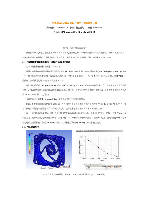
ANSYSWORKBENCH疲劳分析指南第三章发表时间:2009-2-21 作者: 安世亚太来源: e-works关键字: CAE ansys Workbench疲劳分析第三章不稳定振幅的疲劳在前面一章中,考察了恒定振幅和比例载荷的情况,并涉及到最大和最小振幅在保持恒定的情况下的循环或重复载荷。
在本章将针对不定振幅、比例载荷情况,尽管载荷仍是成比例的,但应力幅和平均应力却是随时间变化的。
3.1 不规律载荷的历程和循环(History and Cycles)对于不规律载荷历程,需要进行特殊处理:计算不规律载荷历程的循环所使用的是“雨流”rainflow循环计算,“雨流”循环计算(Rainflowcycle counting)是用于把不规律应力历程转化为用于疲劳计算的循环的一种技术(如右面例子),先计算不同的“平均”应力和应力幅(“range”)的循环,然后使用这组“雨流”循环完成疲劳计算。
损伤累加是通过Palmgren-Miner 法则完成的,Palmgren-Miner法则的基本思想是:在一个给定的平均应力和应力幅下,每次循环用到有效寿命占总和的百分之几。
对于在一个给定应力幅下的循环次数Ni,随着循环次数达到失效次数Nfi时,寿命用尽,达到失效。
“雨流”循环计算和Palmgren-Miner损伤累加都用于不定振幅情况。
因此,任何任意载荷历程都可以切分成一个不同的平均值和范围值的循环阵列(“多个竖条”),右图是“雨流”阵列,指出了在每个平均值和范围值下所计算的循环次数,较高值表示这些循环的将出现在载荷历程中。
在一个疲劳分析完成以后,每个“竖条”(即“循环”)造成的损伤量将被绘出,对于“雨流”阵列中的每个“竖条”(bin),显示的是对应的所用掉的寿命量的百分比。
在这个例子中,即使大多数循环发生在低范围/平均值,但高范围(range)循环仍会造成主要的损伤。
依据Per Miner法则,如果损伤累加到1(100%),那么将发生失效。
Fatigue_ANSYS疲劳分析
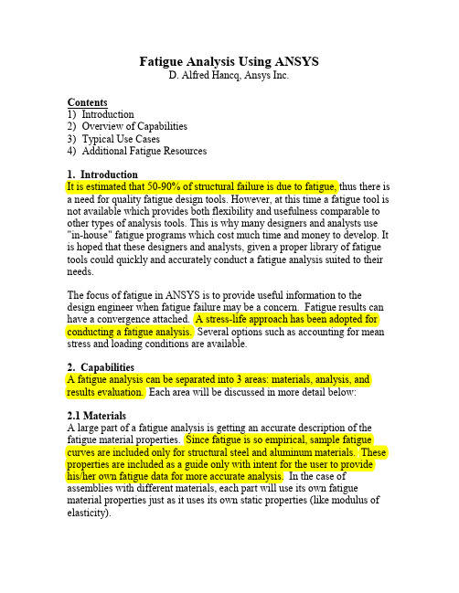
Fatigue Analysis Using ANSYSD. Alfred Hancq, Ansys Inc.Contents1) Introduction2) Overview of Capabilities3) Typical Use Cases4) Additional Fatigue Resources1. IntroductionIt is estimated that 50-90% of structural failure is due to fatigue, thus there is a need for quality fatigue design tools. However, at this time a fatigue tool is not available which provides both flexibility and usefulness comparable to other types of analysis tools. This is why many designers and analysts use "in-house" fatigue programs which cost much time and money to develop. It is hoped that these designers and analysts, given a proper library of fatigue tools could quickly and accurately conduct a fatigue analysis suited to their needs.The focus of fatigue in ANSYS is to provide useful information to the design engineer when fatigue failure may be a concern. Fatigue results can have a convergence attached. A stress-life approach has been adopted for conducting a fatigue analysis. Several options such as accounting for mean stress and loading conditions are available.2. CapabilitiesA fatigue analysis can be separated into 3 areas: materials, analysis, and results evaluation. Each area will be discussed in more detail below:2.1 MaterialsA large part of a fatigue analysis is getting an accurate description of the fatigue material properties. Since fatigue is so empirical, sample fatigue curves are included only for structural steel and aluminum materials. These properties are included as a guide only with intent for the user to provide his/her own fatigue data for more accurate analysis. In the case of assemblies with different materials, each part will use its own fatigue material properties just as it uses its own static properties (like modulus of elasticity).2.1.1 Stress-life Data Options/Features• Fatigue material data stored as tabular alternating stress vs. life points.• The ability to define mean stress dependent or multiple r-ratio curves if the data is available.• Options to have log-log, semi-log, or linear interpolation.• Ability to graphically view the fatigue material data• The fatigue data is saved in XML format along with the other static material data.• Figure 1 is a screen shot showing a user editing fatigue data in ANSYS.Figure 1: Editing SN curves in ANSYS2.2 AnalysisFatigue results can be added before or after a stress solution has been performed. To create fatigue results, a fatigue tool must first be inserted into the tree. This can be done through the solution toolbar or through context menus. The details view of the fatigue tool is used to define the various aspects of a fatigue analysis such as loading type, handling of mean stress effects and more. As seen in Figure 2, a graphical representation of the loading and mean stress effects is displayed when a fatigue tool is selected by the user. This can be very useful to help a novice understand the fatigue loading and possible effects of a mean stress.Figure 2: Fatigue tool information page in ANSYS2.2.1 LoadingFatigue, by definition, is caused by changing the load on a component over time. Thus, unlike the static stress safety tools, which perform calculations for a single stress, fatigue damage occurs when the stress at a point changes over time. ANSYS can perform fatigue calculations for either constant amplitude loading or proportional non-constant amplitude loading. A scale factor can be applied to the base loading if desired. This option, located under the “Loading” section in the details view, is useful to see the effects of different finite element load magnitudes without having to re-run the stress analysis.• Constant amplitude, proportional loading: This is the classic, “backof the envelope” calculation. Loading is of constant amplitude becauseonly 1 set of finite element stress results along with a loading ratio is required to calculate the alternating and mean stress. The loading ratio is defined as the ratio of the second load to the first load (LR = L2/L1).Loading is proportional since only 1 set of finite element stress results is needed (principal stress axes do not change over time). No cumulative damage calculations need to be done. Common types of constantamplitude loading are fully reversed (apply a load then apply an equal and opposite load; a load ratio of –1) and zero-based (apply a load then remove it; a load ratio of 0). Fully reversed, zero-based, or a specified loading ratio can be defined in the details view under the “Loading”section.• Non-constant amplitude, proportional loading: In this case, again only 1 set of results are needed, however instead of using a single load ratio to calculate the alternating and mean stress, the load ratio varies over time. Think of this as coupling an FEM analysis with strain-gauge results collected over a given time interval. Cumulative damagecalculations including cycle counting and damage summation need to be done. A rainflow cycle counting method is used to identify stressreversals and Miner’s rule is used to perform the damage summation.The load scaling comes from an external data file provided by the user, (such as the one in Figure 3) and is simply a list of scale factors.Figure 3: Chart of loading historySeveral sample load histories can be found in the “Load Histories” directory under the “Engineering Data” folder. Setting the loading type to “History Data” in the fatigue tool details view specifies non-constant amplitude loading. Several analysis options are available for non-constant amplitude loading. Since rainflow counting is used, using a “quick counting” technique substantially reduces runtime and memory. In quick counting, alternating and mean stresses are sorted into bins before partial damage is calculated. Without quick counting, the data is not sorted into bins until afterpartial damages are found. Theaccuracy of quick counting isusually very good if a propernumber of bins is used whencounting. The default setting forthe number of bins can be set inthe Control Panel. Turning offquick counting is notrecommended and in fact is nota documented feature. To allowquick counting to be turned off, set the variable “AllowQuickCounting” to 1 in the Variable Manager. Another available option when conducting a variable amplitude fatigue analysis is the ability to set the value used for infinite life. In constant amplitude loading, if the alternating stress is lower than the lowest alternating stress on the fatigue curve, ANSYS will use the life at the last point. This provides for an added level of safety because many materials do not exhibit an endurance limit. However, in non-constant amplitude loading, cycles with very small alternating stresses may be present and may incorrectly predict too much damage if the number of the small stress cycles is high enough. To help control this, the user can set the infinite life value that will be used if the alternating stress is beyond the limit of the SN curve. Setting a higher value will make small stress cycles less damaging if they occur many times. The rainflow and damage matrix results can be helpful in determining the effects of small stress cycles in your loading history. The rainflow and damage matrices shown in Figure 4 illustrate the possible effects of infinite life. Both damage matrices came from the same loading (and thus same rainflow matrix), but the first damage matrix was calculated with an infinite life if 1e6 cycles and the second was calculated with an infinite life of 1e9 cycles.Rainflow matrix for ahistory.loadgivenDamage matrix with an infinitelife of 1e6 cycles. Total damageis calculated to be .19 .Damage matrix with aninfinite life of 1e9 cycles.Total damage is calculatedto be .12 (37% less damage)Figure 4: Effect of infinite life on fatigue damage2.2.2 Load EffectsFatigue material tests are usually conducted in a uniaxial loading under a fixed or zero mean stress state. It is cost-prohibitive to conduct experiments that capture all mean stress, loading, and surface conditions. Thus, empirical relations are available if the fatigue data is not.• Mean Stress correction. If the loading is other than fully reversed, a mean stress exists and should be accounted for. Methods for handling mean stress effects can be found in the “Options” section.If experimental data atdifferent mean stresses or r-ratio’s exist, mean stress canbe accounted for directlythrough interpolation betweenmaterial curves. Ifexperimental data is notavailable, several empiricaloptions may be chosenincluding Gerber, Goodmanand Soderberg theories whichuse static material properties(yield stress, tensile strength)along with S-N data to account for any mean stress. In general, mostexperimental data fall between the Goodman and Gerber theories with the Soderberg theory usually being over conservative. The Goodman theory can be a good choice for brittle materials with the Gerber theory usually a good choice for ductile materials. As can be seen from thescreen shots in Figure 5, the Gerber theory treats negative and positive mean stresses the same whereas Goodman and Soderberg do not apply any correction for negative mean stresses. This is because although a compressive mean stress can retard fatigue crack growth, ignoring anegative mean is usually more conservative. The selected mean stress theory is shown graphically in the display window as seen below. Note that if an empirical mean stress theory is chosen and multiple SN curves are defined, any mean stresses that may exist will be ignored whenquerying the material data since an empirical theory was chosen. Thus if you have multiple r-ratio SN curves and use the Goodman theory, the SN curve at r=-1 will be used. In general it is not advisable to use anempirical mean stress theory if multiple mean stress data exists.Figure 5: The chosen mean stress theory is illustrated in the graphics window• Multiaxial Stress Correction . Experimental test data is uniaxial whereas stresses are usually multiaxial. At some point stress must beconverted from a multiaxial stress state to a uniaxial one. Von-Mises, Max shear, Maximum principal stress, or any of the component stresses can be used as the uniaxial stress value. In addition, a “signed” Von-Mises stress may be chosen where the Von-Mises stress takes the sign of the largest absolute principal stress. This is useful to identify any compressive mean stresses since several of the mean stress theories treatpositive and negative mean stresses differently. Setting the “StressComponent” is done in the Options section in the fatigue tool detail view.2.2.3 Miscellaneous Analysis optionsFatigue material property tests are usually conducted under very specific and controlled conditions (eg. axial loading, polished specimens, .5 inch gauge diameter). If the service part conditions differ from as tested, modification factors can be applied to try to account for the difference. The fatigue alternating stress is usually divided by this modification factor and can be found in design handbooks. (Dividing the alternating stress is equivalent to multiplying the fatigue strength by K f.) The fatigue strength reduction factor is defined by setting “Fatigue Strength Factor (K f)” in the details view for the fatigue tool. Note that this factor is applied to the alternating stress only and does not affect the mean stress.2.3 Results OutputSeveral results for evaluating fatigue are available to the user. Some are contour plots of a specific result over the model while others give information about the most damaged point in the model(or the most damage, factor of safety, stress biaxiality, fatigue sensitivity, rainflow matrix, and damage matrix output. Each output will now be described in detail.• A contour plot of available life over the model. This result can be over the whole model or scoped to a given part or surface. This result contour plot shows the available life for the given fatigue analysis. If loading is of constant amplitude, this represents the number of cycles until the part will fail due to fatigue. If loading is non-constant, this represents thenumber of loading blocks until failure. Thus if the given load historyrepresents one month of loading and the life was found to be 120, theexpected model life would be 120 months. In a constant amplitudeanalysis, if the alternating stress is lower than the lowest alternating stress defined in the S-N curve, the life at that point will be used. See section2.2.1 for more information about the difference between constant andnon-constant amplitude loading.• A contour plot of the fatigue damage at a given design life. Fatigue damage is defined as the design life divided by the available life. This result may be scoped. The default design life may be set through the Control Panel.• A contour plot of the factor of safety with respect to a fatigue failure at a given design life. The maximum FS reported is 15. Like damage and life, this result may be scoped. This calculation is iterative for non-constant amplitude loading and may substantially increase solve time.• A stress biaxiality contour plot over the model. As mentioned previously, material properties are uniaxial but stress results are usually multiaxial. This result gives the user some idea of the stress state over the model and how to interpret the results. Biaxiality indication isdefined as the principal stress smaller in magnitude divided by the larger principal stress with the principal stress nearest zero ignored. Abiaxiality of zero corresponds to uniaxial stress, a value of –1corresponds to pure shear, and a value of 1 corresponds to a pure biaxial state. From the sample biaxiality plot shown below, most of the model is under a pure shear or uniaxial stress. This is expected since a simpletorque has been applied at the top of the model. When using thebiaxiality plot along with the safety factor plot above, it can be seen that the most damaged point occurs at a point of nearly pure shear. Thus it would be desirable to use S-N data collected through torsional loading if available. Of course collecting experimental data under different loading conditions is cost prohibitive and not often done.• A fatigue sensitivity plot. This plot shows how the fatigue results change as a function of the loading at the critical location on the model. This result may be scoped to parts or surfaces. Sensitivity may be found for life, damage, or factory of safety.The user may set the number of fillpoints as well as the load variationlimits. For example, the user maywish to see the sensitivity of themodel’s life if the load was 50% ofthe current load up to if the load150% of the current load. (The x-value of 1 on the graph correspondsto the life at the current loading ofthe model; The x-value at 1.5corresponds to the critical fatiguelife if the finite element loads were 50% higher then they are currently, etc…). Negative variations are allowed in order to see the effects of a possible negative mean stress if the loading is not totally reversed.Linear, Log-X, Log-Y, or Log-Log scaling can be chosen for chartdisplay. Default values for the sensitivity options may be set through the Control Panel.• A plot of the rainflow matrix for the critical location. This result is only applicable for non-constant amplitude loading where rainflow counting is needed. This result may be scoped. In this 3-D histogram, alternating and mean stress is divided into bins and plotted. The Z-axis corresponds to the number of counts for a given alternating and mean stress bin. This result gives the user a measure of the composition of a loading history.(Such as if most of the alternating stress cycles occur at a negative mean stress.) From the rainflow matrix below, the user can see that most of the alternating stresses have a positive mean stress and that bulk of thesmaller alternating stresses have a higher mean stress then the largeralternating stresses.• A plot of the damage matrix at the critical location on the model. This result is only applicable for non-constant amplitude loading whererainflow counting is needed. This result may be scoped. This result is similar to the rainflow matrix except the %damage that each bin caused is plotted as the Z-axis. As can be seen from the corresponding damage matrix for the above rainflow matrix, in this particular case althoughmost of the counts occur at the lower stress amplitudes, most of thedamage occurs at the higher stress amplitudes.3. Typical Use CasesScenario I, Connecting Rod under fully reversed loading: Here we have a connecting rod in a compressor under fully reversed loading (load is applied, removed, then applied in the opposite direction with a max loading of 1000 pounds).• Import geometry and apply boundary conditions. Apply loading corresponding to the maximum developed load of 1000 pounds.• Insert fatigue tool.• Specify fully reversedloading to createalternating stress cycles.• Specify that this is astress-life fatigueanalysis. No meanstress theory needs to bespecified since no meanstress will exist (fullyreversed loading). Specify that Von-Mises stress will be used to compare against fatigue material data.• Specify a modification factor of .8 since material data represents a polished specimen and the in-service component is cast.• Perform stress and fatigue calculations (Solve command in context menu).• Plot factor of safety for a design life of 1,000,000 cycles.• Find the sensitivity of available life with respect to loading. Specify a minimum base load variation of 50% (an alternating stress of 500 lbs.) and a maximum base load variation of 200% (an alternating stress of 2000 lbs.)• Determine multiaxial stress state (uniaxial, shear, biaxial, or mixed) at critical life location by inserting “biaxiality indicator” into fatiguetool. The stress state near the critical location is not far from uniaxial (.1~.2), which gives and added measure of confidence since thematerial properties are uniaxial.Scenario II, Connecting Rod under random loading: Here we have the same connecting rod and boundary conditions but the loading is not of a constant amplitude over time. Assume that we have strain gauge results that were collected experimentally from the component and that we know that a strain gauge reading of 200 corresponds to an applied load of 1,000 pounds. • Conduct the static stress analysis as before using a load of 1,000 pounds.• Insert fatigue tool. • Specify fatigue loading as coming from a scale history and select scale history file containing strain gauge results over time(ex. Common Files\Ansys Inc\Engineering Data\Load Histories\SAEBracketHistory.dat ). Define the scale factor to be .005. (We must normalize the loadhistory so that the FEM load matches the scale factors in the load history file).factor scale load needed gauge strain 200load FEM 1gauge strain 20010001000load FEM 1== × lbs lbs •Specify a bin size of 32 (Rainflow and damage matrices will be of dimension 32x32). •Specify Goodman theory to account for mean-stress effects. (The chosen theory will be illustrated graphically in the graphics window. Specify that a signed Von-Mises stress will be used to compare against fatigue material data. (Use signed since Goodman theory treats negative and positive mean stresses differently.) • Perform fatigue calculations (Solve command in context menu). • View rainflow and damage matrix.• Plot life, damage, and factor of safety contours over the model at a design life of 1000. (The fatigue damage and FS if this loading history was experienced 1000 times). Thus if the loading historycorresponded to the loading experienced by the part over a month’s time, the damage and FS will be at a design life of 1000 months. Note that although a life of only 88 loading blocks is calculated, the needed scale factor (since FS@1000=.61) is only .61 to reach a life of 1000 blocks.• Plot factor of safety as a function of the base load (fatigue sensitivity plot, a 2-D XY plot).• Copy and paste to create another fatigue tool and specify that mean stress effects will be ignored (SN-None theory) This will be done to ascertain to what extent mean stress is affecting fatigue life.• Perform fatigue calculations.• View damage and factor of safety and compare results obtained when using Goodman theory to get the extent of any possible mean stress effect.• Change bin size to 50, rerun analysis, and compare fatigue results to verify that the bin size of 32 was of adequate size to get desiredprecision for alternating and mean stress bins.4. Additional fatigue resources• Hancq, D.A., Walters, A.J., Beuth, J.L., “Development of an Object-Oriented Fatigue Tool”, Engineering with Computers, Vol 16, 2000,pp. 131-144.This paper gives details on both the underlying structure andengineering aspects of the fatigue tool used by the DesignSpaceprogram.• Bannantine, J., Comer, J., Handrock, J. “Fundamentals of Metal Fatigue Analysis”, New Jersey, Prentice Hall (1990).This is an excellent book that explains the fundamentals of fatigue to a novice user. Many topics such as mean stress effects and rainflowcounting are topics in this book.• Lampman, S.R. editor, “ASM Handbook: Volume 19, Fatigue and Fracture”, ASM International (1996).Good reference to have when conducting a fatigue analysis. Contains papers on a wide variety of fatigue topics.• U.S. Dept. of Defense, “MIL-HDBK-5H: “Metallic materials and Elements for Aerospace Vehicle Structures”, (1998).This publication distributed by the United States government givesfatigue material properties of several common engineering alloys. Itis freely downloadable over the Internet from the NASA website.</FEMCI/links.html>。
ansys-workbench疲劳分析流程

ansys workbench疲劳分析流程基于S-N曲线的疲劳分析的最终目的是将变化无规律的多轴应力转化为简单的单轴应力循环,以便查询S-N曲线,得到相应的疲劳寿命。
ansysworkbench 的疲劳分析模块采用如下流程,其中r=Smin/Smax,Sa为应力幅度,Sm应力循环中的应力均值,注意后一个m不是大写:):(1)无规律多轴应力-->无规律单轴应力这个转换其实就是采用何种应力(或分量)。
只能有以下选择:Von-Mises等效应力;最大剪应力;最大主应力;或某一应力分量(Sx,Syz 等等)。
有时也采用带符号的Mises应力(大小不变等于Mises应力,符号取最大主应力的符号,好处是可以考虑拉或压的影响(反映在平均应力或r上))。
同强度理论类似,Von-Mises等效应力和最大剪应力转换适用于延展性较好的材料,最大主应力转换用于脆性材料。
(2)无规律单轴应力-->简单单轴应力循环其本质是从无规律的高高低低的等效单轴应力--时间曲线中提取出一系列的简单应力循环(用Sa,Sm表征)以及对应的次数。
有很多种方法可以完成此计数和统计工作,其中又分为路径相关方法和路径无关方法。
用途最广的雨流法(rainflowcountingmethod)就是一种路径相关方法。
其算法和原理可见“Downing, S., Socie, D. (1982) Simplified rain flow counting algorithms. Int J Fatigue,4, 31–40“。
经过雨流法的处理后,无规律的应力--时间曲线转化为一系列的简单循环(Sa,Sm和ni,ni为该循环的次数,Sm如果不等于0,即r!=-1,需要考虑r的影响)。
然后将r!=-1的循环再转化到r=-1对应的应力循环(见下),这样就可以根据损伤累计理论(Miner准则)计算分析了:Sum(ni/Ni) Ni为该应力循环对应的寿命(考虑Sa,Sm)。
ANSYS疲劳分析介绍

3.1 疲劳的定义疲劳是指结构在低于静态极限强度载荷的重复载荷作用下,出现断裂破坏的现象。
例如一根能够承受300 KN 拉力作用的钢杆,在200 KN 循环载荷作用下,经历1,000,000 次循环后亦会破坏。
导致疲劳破坏的主要因素如下:载荷的循环次数;每一个循环的应力幅;每一个循环的平均应力;存在局部应力集中现象。
真正的疲劳计算要考虑所有这些因素,因为在预测其生命周期时,它计算“消耗”的某个部件是如何形成的。
3.1.1 ANSYS程序处理疲劳问题的过程ANSYS 疲劳计算以ASME锅炉和压力容器规范(ASME Boiler and Pressure Vessel Code)第三节(和第八节第二部分)作为计算的依据,采用简化了的弹塑性假设和Mimer累积疲劳准则。
除了根据ASME 规范所建立的规则进行疲劳计算外,用户也可编写自己的宏指令,或选用合适的第三方程序,利用ANSYS 计算的结果进行疲劳计算。
《ANSYS APDL Programmer…s Guide》讨论了上述二种功能。
ANSYS程序的疲劳计算能力如下:对现有的应力结果进行后处理,以确定体单元或壳单元模型的疲劳寿命耗用系数(fatigue usage factors)(用于疲劳计算的线单元模型的应力必须人工输入);可以在一系列预先选定的位置上,确定一定数目的事件及组成这些事件的载荷,然后把这些位置上的应力储存起来;可以在每一个位置上定义应力集中系数和给每一个事件定义比例系数。
3.1.2 基本术语位置(Location):在模型上储存疲劳应力的节点。
这些节点是结构上某些容易产生疲劳破坏的位置。
事件(Event):是在特定的应力循环过程中,在不同时刻的一系列应力状态,见本章§3.2.3.4。
载荷(Loading):是事件的一部分,是其中一个应力状态。
应力幅:两个载荷之间应力状态之差的度量。
程序不考虑应力平均值对结果的影响。
3.2 疲劳计算完成了应力计算后,就可以在通用后处理器POST1 中进行疲劳计算。
ANSYS疲劳分析

ANSYS疲劳分析ANSYS是一种流行的工程仿真软件,用于进行各种工程问题的有限元分析。
在工程实践中,疲劳分析是一个非常重要的领域。
疲劳是指材料在重复载荷作用下逐渐破坏的过程。
疲劳分析的目的是评估结构在实际使用条件下的寿命和性能。
ANSYS可以用来进行疲劳分析,通过确定应力和应变的分布,评估结构在长期使用中可能出现的问题。
在进行疲劳分析之前,首先要进行有限元模型的建立。
这包括将结构模型导入到ANSYS中,确定边界条件和加载条件等。
在进行疲劳分析时,首先要确定疲劳载荷的类型和大小。
这可以通过实验测量或数值模拟来获取。
然后,将载荷应用在结构模型上,并进行动态分析。
ANSYS可以模拟不同的载荷情况,例如正弦载荷、随机载荷和脉冲载荷等。
通过分析结果,可以获得结构在不同位置的应力和应变分布。
在完成动态分析后,可以对结果进行验证和修正。
如果分析的结果与实际测量不符,可能需要对模型进行修正。
修正的方法包括调整材料的本构模型、改变模型的几何形状或重新定义载荷条件等。
完成验证后,可以进行疲劳分析。
在ANSYS中,可以使用不同的疲劳分析模块进行分析。
其中最常用的是疲劳寿命评估模块。
该模块可以根据疲劳参数和材料的S-N曲线,预测结构在给定载荷下的疲劳寿命。
这可以帮助工程师评估结构的安全性和可靠性,并采取适当的措施来延长结构的使用寿命。
疲劳分析还可以进行应力寿命曲线分析。
该分析方法可以通过建立不同应力水平和循环数的组合,预测结构的疲劳寿命。
这对于识别结构中的关键部位和进行寿命预测非常有帮助。
此外,还可以使用应变寿命方法进行疲劳分析。
该方法通过应变历程和损伤累积,评估结构在疲劳载荷下的性能。
在完成疲劳分析后,可以对结果进行后处理。
这包括评估结构的疲劳寿命、疲劳裕度和故障位置等。
通过分析结果,可以确定哪些部位可能会在疲劳过程中发生破坏,并采取适当的措施来加强这些部位。
总之,ANSYS是进行疲劳分析的强大工具。
它可以用于建立结构模型、应用载荷、进行动态分析和预测结构的疲劳寿命。
ANSYS疲劳分析介绍
3.1 疲劳的定义疲劳是指结构在低于静态极限强度载荷的重复载荷作用下,出现断裂破坏的现象。
例如一根能够承受300 KN 拉力作用的钢杆,在200 KN 循环载荷作用下,经历1,000,000 次循环后亦会破坏。
导致疲劳破坏的主要因素如下:载荷的循环次数;每一个循环的应力幅;每一个循环的平均应力;存在局部应力集中现象。
真正的疲劳计算要考虑所有这些因素,因为在预测其生命周期时,它计算“消耗”的某个部件是如何形成的。
3.1.1 ANSYS程序处理疲劳问题的过程ANSYS 疲劳计算以ASME锅炉和压力容器规范(ASME Boiler and Pressure Vessel Code)第三节(和第八节第二部分)作为计算的依据,采用简化了的弹塑性假设和Mimer累积疲劳准则。
除了根据ASME 规范所建立的规则进行疲劳计算外,用户也可编写自己的宏指令,或选用合适的第三方程序,利用ANSYS 计算的结果进行疲劳计算。
《ANSYS APDL Programmer…s Guide》讨论了上述二种功能。
ANSYS程序的疲劳计算能力如下:对现有的应力结果进行后处理,以确定体单元或壳单元模型的疲劳寿命耗用系数(fatigue usage factors)(用于疲劳计算的线单元模型的应力必须人工输入);可以在一系列预先选定的位置上,确定一定数目的事件及组成这些事件的载荷,然后把这些位置上的应力储存起来;可以在每一个位置上定义应力集中系数和给每一个事件定义比例系数。
3.1.2 基本术语位置(Location):在模型上储存疲劳应力的节点。
这些节点是结构上某些容易产生疲劳破坏的位置。
事件(Event):是在特定的应力循环过程中,在不同时刻的一系列应力状态,见本章§3.2.3.4。
载荷(Loading):是事件的一部分,是其中一个应力状态。
应力幅:两个载荷之间应力状态之差的度量。
程序不考虑应力平均值对结果的影响。
3.2 疲劳计算完成了应力计算后,就可以在通用后处理器POST1 中进行疲劳计算。
(完整版)疲劳分析的数值计算方法及ANSYS疲劳分析实例

第十四章疲劳分析的数值计算方法及实例第一节引言零件或构件由于交变载荷的反复作用,在它所承受的交变应力尚未达到静强度设计的许用应力情况下就会在零件或构件的局部位置产生疲劳裂纹并扩展、最后突然断裂。
这种现象称为疲劳破坏。
疲劳裂纹的形成和扩展具有很大的隐蔽性而在疲劳断裂时又具有瞬发性,因此疲劳破坏往往会造成极大的经济损失和灾难性后果。
金属的疲劳破坏形式和机理不同与静载破坏,所以零件疲劳强度的设计计算不能为经典的静强度设计计算所替代,属于动强度设计。
随着机车车辆向高速、大功率和轻量化方向的迅速发展,其疲劳强度及其可靠性的要求也越来越高。
近几年随着我国铁路的不断提速,机车、车辆和道轨等铁路设施的疲劳断裂事故不断发生,越来越引起人们的重视。
疲劳强度设计及其研究正在成为我国高速机车车辆设计制造中的一项不可缺少的和重要的工作。
金属疲劳的研究已有近150年的历史,有相当多的学者和工程技术人员进行了大量的研究,得到了许多关于金属疲劳损伤和断裂的理论及有关经验技术。
但是由于疲劳破坏的影响因素多而复杂并且这些因素互相影响又与构件的实际情况密切相关,使得其应用性成果尚远远不能满足工程设计和生产应用的需要。
据统计,至今有约90%的机械零部件的断裂破坏仍然是由直接于疲劳或者间接疲劳而引起的。
因此,在21世纪的今天,尤其是在高速和大功率化的新产品的开发制造中,其疲劳强度或疲劳寿命的设计十分重要,并且往往需要同时进行相应的试验研究和试验验证。
疲劳断裂是因为在零件或构件表层上的高应力或强度比较低弱的部位区域产生疲劳裂纹,并进一步扩展而造成的。
这些危险部位小到几个毫米甚至几十个微米的范围,零件或构件的几何缺口根部、表面缺陷、切削刀痕、碰磕伤痕及材料的内部缺陷等往往是这种危险部位。
因此,提高构件疲劳强度的基本途径主要有两种。
一种是机械设计的方法,主要有优化或改善缺口形状,改进加工工艺工程和质量等手段将危险点的峰值应力降下来;另一种是材料冶金的方法,即用热处理手段将危险点局部区域的疲劳强度提高,或者是提高冶金质量来减少金属基体中的非金属夹杂等材料缺陷等局部薄弱区域。
- 1、下载文档前请自行甄别文档内容的完整性,平台不提供额外的编辑、内容补充、找答案等附加服务。
- 2、"仅部分预览"的文档,不可在线预览部分如存在完整性等问题,可反馈申请退款(可完整预览的文档不适用该条件!)。
- 3、如文档侵犯您的权益,请联系客服反馈,我们会尽快为您处理(人工客服工作时间:9:00-18:30)。
线模型目前还不能输出应力结果,所以疲劳计算对于线是忽略的.
– 线仍然可以包括在模型中以给结构提供刚性, 但在疲劳分析并不计算 线模型
ANSYS License Fatigue Module DesignSpace Entra DesignSpace Professional Structural Mechanical/Multiphysics
σmax σmin
February 20, 2004 Inventory #002018 14-6
疲劳模块
… 应力-寿命曲线
•
培训手朋
ANSYS Workbench – Simulation ANSYS Workbench – Simulation ANSYS Workbench – Simulation ANSYS Workbench – Simulation
– 否则,则称为变化振幅或非恒定振幅 载荷 (本章之后将给予讨论).
February 20, 2004 Inventory #002018 14-4
疲劳模块
… 成比例载荷
•
培训手朋
ANSYS Workbench – Simulation ANSYS Workbench – Simulation ANSYS Workbench – Simulation ANSYS Workbench – Simulation
ANSYS Workbench 疲劳分析
疲劳绍疲劳模块拓展功能的使用:
– 使用者要先学习第4章线性静态结构分析.
培训手朋
ANSYS Workbench – Simulation ANSYS Workbench – Simulation ANSYS Workbench – Simulation ANSYS Workbench – Simulation
– 一个部件通常经受多轴应力状态.如果疲劳数据(S-N 曲线)是从反映 单轴应力状态的测试中得到的,那么在计算寿命时就要注意
• 设计仿真为用户提供了如何把结果和S-N 曲线相关联的选择,包括多轴应 力的选择 • 双轴应力结果有助于计算在给定位置的情况
– 平均应力影响疲劳寿命,并且变换在S-N曲线的上方位置与下方位置 ( 反映出在给定应力幅下的寿命长短)
疲劳模块
A. 疲劳概述
• • 结构失效的一个常见原因是疲劳,其造成破坏与重复加载有关
培训手朋
ANSYS Workbench – Simulation ANSYS Workbench – Simulation ANSYS Workbench – Simulation ANSYS Workbench – Simulation
对压缩和拉伸平均应力,平均应力将分别提高和降低S-N曲线.
February 20, 2004 Inventory #002018 14-8
疲劳模块
…应力-寿命曲线
• 因此,记住以下几点:
培训手朋
ANSYS Workbench – Simulation ANSYS Workbench – Simulation ANSYS Workbench – Simulation ANSYS Workbench – Simulation
考虑在最大最小应力值σmin 和 σmax作用下的比例载荷、恒定振幅 的情况: – 应力范围 Δσ 定义为 (σmax- σmin) – 平均应力 σm 定义为 (σmax+σmin)/2 – 应力幅或交变应力 σa是Δσ/2
– 应力比 R 是 σmin/ σmax – 当施加的是大小相等且方向相反的载荷时,发生的是对称循环载荷. 这就是σm = 0 ,R = -1的情况. – 当施加载荷后又撤除该载荷,将发生脉动循环载荷. 这就是 σm = σmax/2 , R = 0的情况.
… 恒定振幅载荷
• 在前面曾提到, 疲劳是由于重复加载 引起:
– 当最大和最小的应力水平恒定时, 称 为恒定振幅载荷. 我们将针对这种最 简单的形式,首先进行讨论.
培训手朋
ANSYS Workbench – Simulation ANSYS Workbench – Simulation ANSYS Workbench – Simulation ANSYS Workbench – Simulation
•
在设计仿真中, 疲劳模块拓展程序( Fatigue Module add-on) 采用的是基于应力疲劳(stress-based)理论,它适用于高周疲 劳. 接下来,我们将对基于应力疲劳理论的处理方法进行讨论.
February 20, 2004 Inventory #002018 14-3
疲劳模块
载荷可以是比例载荷, 也可以非比例载荷: – 比例载荷, 是指主应力的比例是恒定的,并且主应力的削减不随时间 变化. 这实质意味着由于载荷的增加或反作用的造成的响应很容易
得到计算. – 相反, 非比例载荷没有隐含各应力之间 相互的关系,典型情况包括:
• 在两个不同载荷工况间的交替变化 • 交变载荷叠加在静载荷上 • 非线性边界条件
疲劳模块
… 总结
• •
培训手朋
ANSYS Workbench – Simulation ANSYS Workbench – Simulation ANSYS Workbench – Simulation ANSYS Workbench – Simulation
疲劳模块允许用户采用基于应力理论的处理方法,来解决高周疲 劳问题. 以下情况可以用疲劳模块来处理:
σ2 = constant σ1
February 20, 2004 Inventory #002018 14-5
疲劳模块
… 应力定义
•
培训手朋
ANSYS Workbench – Simulation ANSYS Workbench – Simulation ANSYS Workbench – Simulation ANSYS Workbench – Simulation
对数显示
上述数据曲线,分别是用线性与对数来表示的. 由于数据的本质原因, 采用对数绘制曲线,往往 能更方便地查看S-N曲线的情况.
February 20, 2004 Inventory #002018 14-7
疲劳模块
…应力-寿命曲线
• S-N曲线是通过对试件做疲劳测试得到的
– 弯曲或轴向测试反映的是单轴的应力状态 – 影响S-N 曲线的因素很多, 其中的一些需要的注意,如下: – 材料的延展性, 材料的加工工艺 – 几何形状信息,包括表面光滑度、残余应力以及存在的应力集中 – 载荷环境, 包括平均应力、温度和化学环境 •
在这部分中将包括以下内容:
– 疲劳概述 – 恒定振幅下的通用疲劳程序,比例载荷情况 比例 – 变振幅下的疲劳程序, 比例载荷情况 比例 – 恒定振幅下的疲劳程序,非比例载荷情况 比例
•
上述功能适用于 ANSYS DesignSpace licenses和 附带疲劳模 块的更高级的licenses.
February 20, 2004 Inventory #002018 14-2
疲劳通常分为两类: – 高周疲劳是当载荷的循环(重复)次数高 (如 1e4 - 1e9)的情况下产
生的. 因此,应力通常比材料的极限强度低. 应力疲劳(Stressbased )用于高周疲劳. – 低周疲劳是在循环次数相对较低时发生的 。塑性变形常常伴随低周 疲劳,其阐明了短疲劳寿命。一般认为应变疲劳(strain-based ) 应该用于低周疲劳计算 .
February 20, 2004 Inventory #002018 14-10
疲劳模块
B. 疲劳程序 (基本情况)
•
培训手朋
ANSYS Workbench – Simulation ANSYS Workbench – Simulation ANSYS Workbench – Simulation ANSYS Workbench – Simulation
Availability x x x x x x
February 20, 2004 Inventory #002018 14-11
疲劳模块
… 疲劳程序
•
培训手朋
ANSYS Workbench – Simulation ANSYS Workbench – Simulation ANSYS Workbench – Simulation ANSYS Workbench – Simulation
载荷与疲劳失效的关系,采用的是应力-寿命曲线或S-N曲线来表 示:
– 若某一部件在承受循环载荷, 经过一定的循环次数后,该部件裂纹或 破坏将会发展,而且有可能导致失效 – 如果同个部件作用在更高的载荷下,导致失效的载荷循环次数将减少 – 应力-寿命曲线或S-N曲线,展示出应力幅与失效循环次数的关系
线性显示
– 在本节中,将涵盖关于恒定振幅、比例载荷的情况. 而变化振幅、比 例载荷的情况和恒定振幅、非比例载荷的情况,将分别在以后的C 和 D节中逐一讨论.
ANSYS License Fatigue Module DesignSpace Entra DesignSpace Professional Structural Mechanical/Multiphysics
•
培训手朋
ANSYS Workbench – Simulation ANSYS Workbench – Simulation ANSYS Workbench – Simulation ANSYS Workbench – Simulation
例如,压缩平均应力比零平均应力的疲劳寿命长,相反,拉伸平均应力 比零平均应力的疲劳寿命短.
进行疲劳分析是基于线性静力分析, 所以不必对所有的步骤进行 详尽的阐述.
– 疲劳分析是在线性静力分析之后,通过设计仿真自动执行的.