c数值分析c6-8
《数值分析》所有参考答案
等价三角方程组
, ,
11.设计算机具有4位字长。分别用Gauss消去法和列主元Gauss消去法解下列方程组,并比较所得的结果。
解:Gauss消去法
回代
列主元Gauss消去
15.用列主元三角分解法求解方程组。其中
A= ,
解:
等价三角方程组
回代得
, , ,
16.已知 ,求 , , 。
解:
, ,
17.设 。证明
,(II)
,
当 时
当 时
迭代格式(II)对任意 均收敛
3) ,
构造迭代格式 (III)
,
当 时
当 时
迭代格式(III)对任意 均收敛
4)
取格式(III)
, , ,
4.用简单迭代格式求方程 的所有实根,精确至有3位有效数。
解:
当 时, ,
1 2
当 时
,
,
, ,
1)
迭代格式 ,
,
当 时, ,
任取 迭代格式收敛于
是中的一种向量范数。
解:
当 时存在 使得
,
,
所给 为 上的一个范数
18.设 。证明
(1) ;
(2) ;
(3) 。
解:(1)
(2)
(3)
19.设
A=
求 , , 及 , 。
解: ,
Newton迭代格式
,
20.设 为 上任意两种矩阵(算子)范数,证明存在常数
, 使得
对一切 均成立。
解:由向量范数的等价性知道存在正常数 使得
,
=0.187622
[23.015625 , 23.015625+0.187622]
c同位素分析
c同位素分析以“C同位素分析”为标题,写一篇3000字的中文文章C同位素分析是一种通过分析物质中C同位素组成,以确定物质成分及原料来源来支撑定量生态学研究的方法,也是研究生物群落结构特征及其变化的一种重要手段。
它是一种独特的工具,可以揭示营养的来源、群落的食物网络特征、物种的食性、捕食者的捕食过程、以及生态网络的调节作用等。
C同位素分析是利用气相色谱-质谱联用设备,以放射性稳定同位素C-12、C-13的质量比做指标,对无机和有机物质中的碳按其生物同位素丰度分析的方法,从而进行识别和定量分析。
C-13定位素在碳物质中的丰度水平是由物质的来源决定的,主要有生物还原和来自工业分配,工业分配的C-13丰度偏低,而生物还原的C-13丰度一般较高,因此,还原的碳源的C-13定位素比值普遍较低,而来自有机物的碳则具有较高的C-13定位素比值。
C同位素分析可以分析物质来源,如有机碳物质来源于植物或动物,而石油、天然气等无机碳物质则来自非生物源。
在分析食物网络中,C同位素分析可以确定消费者在食物链中的位置,从而帮助研究物种特征、个体数目及其饱食度等信息,进而提高营养学研究的准确性。
C同位素分析也可以用于追踪污染物的原料来源。
C同位素分析可以将污染物来源分辨为有机或无机物质,从而比较定位素的比值,以识别污染来源。
此外,C同位素分析可以用于鉴别生物体的季节性变化,以及研究生态系统中物质的健康状态和变化趋势。
例如,碳同位素可以用来确定森林生物群落的碳循环过程,从而了解森林的能量来源和消耗,研究森林碳汇的效应,并进一步推断森林处于保护状态或被破坏状态。
C同位素分析在实际应用中仍然有很多不足,这主要是由于C同位素分析需要购买特殊的设备和贵重的试剂,而且,C同位素分析的过程比较繁琐复杂,分析结果不够准确。
因此,要提高C同位素分析的实用性,还需要更多研究来完善该技术。
总而言之,C同位素分析是一种重要的生态学研究技术,它可以用于物质来源的分析,同时可以分析食物网络的结构,为森林碳汇的研究及污染物的追踪提供定量的信息,然而,其实用性还存在许多不足,需要进一步的改进。
数值分析报告
数值实验报告实验名称:递推计算的稳定性班级:姓名:学号:日期:一、实验课题:计算积分dx xa x I nn ⎰+=1(n=0,1,2,...10) 其中a 为参数,分别对a=10及a=15按下列两种方案计算,列出其结果,并对其可靠性进行分析比较,说明原因。
解:采用如下两种方案: 方案I :用递推公式naI I n n 11+=- (n=0,1,2,...10)递推初值由积分直接求得1ln(0aa I +=。
(1)算法设计:N(2)程序清单:program project1real a,i(10) open(unit=2,file='project1.xls',status='new', $ access='sequential',form='formatted') print*,'请输入参数a 的值' read*,a i(0)=log((a+1.0)/a) write(2,20) a,i(0)20 format(2ha=,f5.2/5hi(0)=,e14.8) do 10 n=1,10 i(n)=-a*i(n-1)+1.0/n write(2,100)n,i(n) 10 continue100 format(2hi(,i2,2h)=,e14.8) close(2) end(3)输出结果: 表方案II :用递推公式)1(11nI a I n n +=- (n=N,N-1, (1)根据估计式 )1(1)1)(1(1+<<++n a I n a n 当1+≥n n a或nI n a n 1)1)(1(1<<++ 当10+<≤n n a 取递推初值为 1)1)(1(212)1(1)1)(1(121+≥∆+++=⎥⎦⎤⎢⎣⎡++++≈N Na N a a a N a N a I NN 当 或 101)1)(1(121+<≤∆⎥⎦⎤⎢⎣⎡+++≈N Na I N N a I NN 当 计算中取N=13开始。
李庆扬-数值分析第五版第6章习题答案(20130819)
试考察解此方程组的雅可比迭代法及高斯-赛德尔迭代法的收敛性。 雅可比迭代的收敛条件是
( J ) ( D 1 ( L U )) 1
高斯赛德尔迭代法收敛条件是
(G ) (( D L) 1U ) 1
因此只需要求响应的谱半径即可。 本题仅解 a),b)的解法类似。 解:
3.设线性方程组
a11 x1 a12 x2 b1 a11 , a12 0 a21 x1 a22 x2 b2
证明解此方程的雅可比迭代法与高斯赛德尔迭代法同时收敛或发散, 并求两种方 法收敛速度之比。 解:
a A 11 a21
则
a12 a22
5. 何谓矩阵 A 严格对角占优?何谓 A 不可约? P190, 如果 A 的元素满足
aij aij ,i=1,2,3….
j 1 j i
n
称 A 为严格对角占优。 P190 设 A (aij )nn (n 2) ,如果存在置换矩阵 P 使得
A PT AP 11 0
x ( k 1) x ( k )
10 4 时迭代终止。
2 1 5 (a)由系数矩阵 1 4 2 为严格对角占优矩阵可知,使用雅可比、高斯 2 3 10
赛德尔迭代法求解此方程组均收敛。[精确解为 x1 4, x 2 3, x3 2 ] (b)使用雅可比迭代法:
2.给出迭代法 x ( k 1) Bx (k ) f 收敛的充分条件、误差估计及其收敛速度。 迭代矩阵收敛的条件是谱半径 ( B0 ) 1 。其误差估计为
1 k
(k) Bk (0)
R ( B) ln B k 迭代法的平均收敛速度为 k
数值分析方法计算定积分
数值分析⽅法计算定积分⽤C语⾔实现⼏种常⽤的数值分析⽅法计算定积分,代码如下:1 #include <stdio.h>2 #include <string.h>3 #include <stdlib.h>4 #include <math.h>56#define EPS 1.0E-14 //计算精度7#define DIV 1000 //分割区间,值越⼤,精确值越⾼8#define ITERATE 20 //⼆分区间迭代次数,区间分割为2^n,初始化应该⼩⼀点,否则会溢出910#define RECTANGLE 0 //矩形近似11#define TRAPEZOID 1 //梯形近似12#define TRAPEZOID_FORMULA 2 //递推梯形公式13#define SIMPSON_FORMULA 3 //⾟普森公式14#define BOOL_FORMULA 4 //布尔公式1516double function1(double);17double function2(double);18double function3(double);19void Integral(int, double f(double), double, double); //矩形, 梯形逼近求定积分公式20void Trapezoid_Formula(double f(double), double a, double b); //递推梯形公式21void Simpson_Formula(double f(double), double a, double b); //⾟普森公式22void Bool_Formula(double f(double), double a, double b); //布尔公式23void Formula(int, double f(double), double, double);2425double function1(double x)26 {27double y;28 y = cos(x);29return y;30 }3132double function2(double x)33 {34double y;35 y=1/x;36// y = 2+sin(2 * sqrt(x));37return y;38 }3940double function3(double x)41 {42double y;43 y = exp(x);44return y;45 }4647int main()48 {49 printf("y=cos(x) , x=[0, 1]\n");50 printf("Rectangle : "); Integral(RECTANGLE, function1, 0, 1);51 printf("Trapezoid : "); Integral(TRAPEZOID, function1, 0, 1);52 Formula(TRAPEZOID_FORMULA, function1, 0, 1);53 Formula(SIMPSON_FORMULA, function1, 0, 1);54 Formula(BOOL_FORMULA, function1, 0, 1);55 printf("\n");5657 printf("y=1/x , x=[1, 5]\n");58 printf("Rectangle : "); Integral(RECTANGLE, function2, 1, 5);59 printf("Trapezoid : "); Integral(TRAPEZOID, function2, 1, 5);60 Formula(TRAPEZOID_FORMULA, function2, 1, 5);61 Formula(SIMPSON_FORMULA, function2, 1, 5);62 Formula(BOOL_FORMULA, function2, 1, 5);63 printf("\n");6465 printf("y=exp(x) , x=[0, 1]\n");66 printf("Rectangle : "); Integral(RECTANGLE, function3, 0, 1);67 printf("Trapezoid : "); Integral(TRAPEZOID, function3, 0, 1);68 Formula(TRAPEZOID_FORMULA, function3, 0, 1);69 Formula(SIMPSON_FORMULA, function3, 0, 1);70 Formula(BOOL_FORMULA, function3, 0, 1);7172return0;73 }74//积分:分割-近似-求和-取极限75//利⽤黎曼和求解定积分76void Integral(int method, double f(double),double a,double b) //f(double),f(x), double a,float b,区间两点77 {79double x;80double sum = 0; //矩形总⾯积81double h; //矩形宽度82double t = 0; //单个矩形⾯积8384 h = (b-a) / DIV;8586for(i=1; i <= DIV; i++)87 {88 x = a + h * i;89switch(method)90 {91case RECTANGLE :92 t = f(x) * h;93break;94case TRAPEZOID :95 t = (f(x) + f(x - h)) * h / 2;96break;97default:98break;99 }100 sum = sum + t; //各个矩形⾯积相加101 }102103 printf("the value of function is %.10f\n", sum);104 }105106//递推梯形公式107void Trapezoid_Formula(double f(double), double a, double b)//递推梯形公式108 {109 unsigned int i, j, M, J=1;110double h;111double F_2k_1 = 0;112double T[32];113double res = 0;114115 T[0] = (f(a) + f(b)) * (b-a)/2;116for(i=0; i<ITERATE; i++)117 {118 F_2k_1 = 0;119 J = 1;120121for(j=0; j<=i; j++) //区间划分122 J <<= 1; //2^J123 h = (b - a) /J; //步长124//M = J/2; //2M表⽰将积分区域划分的块数125for(j=1; j <= J; j += 2) //126 {127 F_2k_1 += f(a + j*h); //f(2k-1)累加和128 }129 T[i+1] = T[i]/2 + h * F_2k_1; //递推公式130 res = T[i+1];131132if(fabs(T[i+1] - T[i]) < EPS)133if(i < 3) continue;134else break;135 }136137 printf("Trapezoid_Formula : the value of function is %.10f\n", res);138//return res;139 }140//⾟普森公式141void Simpson_Formula(double f(double), double a, double b) //⾟普森公式142 {143 unsigned int i, j, M, J=1;144double h;145double F_2k_1 = 0;146double T[32], S[32];147double res_T = 0, res_S = 0;148149 T[0] = (f(a) + f(b)) * (b-a)/2;150for(i=0; i<ITERATE; i++)151 {152 F_2k_1 = 0;153 J = 1;154155for(j=0; j<=i; j++) //区间划分156 J <<= 1; //2^J157 h = (b - a) /J; //步长158//M = J/2; //2M表⽰将积分区域划分的块数159for(j=1; j <= J; j += 2) //160 {161 F_2k_1 += f(a + j*h); //f(2k-1)累加和163 T[i+1] = T[i]/2 + h * F_2k_1; //递推梯形公式164 res_T = T[i+1];165166if(fabs(T[i+1] - T[i]) < EPS)167if(i < 3) continue;168else break;169 }170171for(i=1; i<ITERATE; i++)172 {173 S[i] = (4 * T[i] - T[i-1]) / 3; //递推⾟普森公式174 res_S = S[i];175if(fabs(S[i] - S[i-1]) < EPS)176if(i < 3) continue;177else break;178 }179180 printf("Simpson_Formula : the value of function is %.10f\n", res_S);181//return res_S;182 }183184//布尔公式185void Bool_Formula(double f(double), double a, double b) //布尔公式186 {187 unsigned int i, j, M, J=1;188double h;189double F_2k_1 = 0;190double T[32], S[32], B[32];191double res_T = 0, res_S = 0, res_B;192193 T[0] = (f(a) + f(b)) * (b-a)/2;194for(i=0; i<ITERATE; i++)195 {196 F_2k_1 = 0;197 J = 1;198199for(j=0; j<=i; j++) //区间划分200 J <<= 1; //2^J201 h = (b - a) /J; //步长202//M = J/2; //2M表⽰将积分区域划分的块数203for(j=1; j <= J; j += 2) //204 {205 F_2k_1 += f(a + j*h); //f(2k-1)累加和206 }207 T[i+1] = T[i]/2 + h * F_2k_1; //递推公式208 res_T = T[i+1];209210if(fabs(T[i+1] - T[i]) < EPS)211if(i < 3) continue;212else break;213 }214215for(i=1; i<ITERATE; i++)216 {217 S[i] = (4 * T[i] - T[i-1]) / 3; //递推⾟普森公式218 res_S = S[i];219if(fabs(S[i] - S[i-1]) < EPS)220if(i < 3) continue;221else break;222 }223224for(i=1; i<ITERATE; i++)225 {226 B[i] = (16 * S[i] - S[i-1]) / 15; //递推布尔公式227 res_B = B[i];228if(fabs(B[i] - B[i-1]) < EPS)229if(i < 3) continue;230else break;231 }232233 printf("Bool_Formula : the value of function is %.10f\n", res_B);234//return res_B;235 }236237//采⽤⼆分区间的⽅法迭代,实际运⾏速度很慢238void Formula(int method, double f(double), double a, double b)//递推梯形公式239 {240 unsigned int i, j, M, J=1;241double h;242double F_2k_1 = 0;243double T[32], S[32], B[32];244double res_B = 0, res_S = 0, res_T = 0;247for(i=0; i<ITERATE; i++)248 {249 F_2k_1 = 0;250 J = 1;251252for(j=0; j<=i; j++) //区间划分253 J <<= 1; //2^J254 h = (b - a) /J; //步长255//M = J/2; //2M表⽰将积分区域划分的块数256for(j=1; j <= J; j += 2) //257 {258 F_2k_1 += f(a + j*h); //f(2k-1)累加和259 }260 T[i+1] = T[i]/2 + h * F_2k_1; //递推公式261 res_T = T[i+1];262263if(fabs(T[i+1] - T[i]) < EPS)264if(i < 3) continue;265else break;266 }267268switch(method)269 {270default :271case TRAPEZOID_FORMULA :272 printf("Trapezoid_Formula : the value of function is %.10f\n", res_T); 273//return res_T;274break;275case SIMPSON_FORMULA :276for(i=1; i<ITERATE; i++)277 {278 S[i] = (4 * T[i] - T[i-1]) / 3;279 res_S = S[i];280if(fabs(S[i] - S[i-1]) < EPS)281if(i < 3) continue;282else break;283 }284 printf("Simpson_Formula : the value of function is %.10f\n", res_S); 285//return res_S;286break;287case BOOL_FORMULA :288for(i=1; i<ITERATE; i++)289 {290 S[i] = (4 * T[i] - T[i-1]) / 3;291 res_S = S[i];292if(fabs(S[i] - S[i-1]) < EPS)293if(i < 3) continue;294else break;295 }296for(i=1; i<ITERATE; i++)297 {298 B[i] = (16 * S[i] - S[i-1]) / 15;299 res_B = B[i];300if(fabs(B[i] - B[i-1]) < EPS)301if(i < 3) continue;302else break;303 }304305 printf("Bool_Formula : the value of function is %.10f\n", res_B); 306//return res_B;307break;308 }309310 }测试结果:。
顺层滑坡c、φ值参数分析
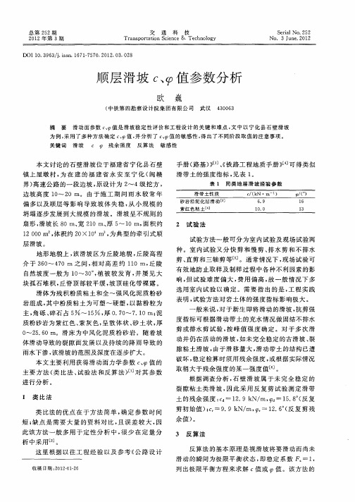
界 ) 速公路 的一 段边 坡 , 设计 为 2 高 原 ~4级 挖方 ,
边 坡高 度 1 ~2 I 由于 施 工 期 间 雨 水 较 常 年 O 0I。 T
偏 多 以及顺 层等 影 响 导 致坡 体 失 稳 , 小 规 模 的 从 坍 塌逐 步发 展到 大规模 的滑坡 。滑坡 呈不 规则 的
扇形 , 滑坡 长 8 宽 2 0m、 5 1 面积 约 Om、 1 厚 ~ 0m,
2 试 验 法
1 0 , 20 0m2体积约 2 ×l T , O O 1。 为典 型的 牵引式 顺 I
层 滑坡 。
试 验方法 一般 可分 为室 内试 验及现 场试验 两 种 。室 内试 验又 分 快 剪 和慢 剪 、 水 剪 和不 排 水 排 剪、 直剪 和三轴 剪等 [ 。通 常情 况下 , 5 ] 现场试 验 可 有 效地 防止取 样及 制样 过程 中各 种不利 因素 的影 响, 但试 验 难 度偏 大 , 费用 偏 高 , 故一 般 情 况下 多
总第 22 5 期 21 0 2年第 3 期
交
通
科
技
Se ilNo. 2 ra 25
Tr n p rain S in e& Te h oo y a s o tt ce c o c n lg
No u e 2 1 .3 J n . 0 2
顺 层 滑 坡 c 值 参 数 分 析 、
选用 室 内试 验 以确 定 。需 要 指 出的 是 , 程 实 践 工
地形 地 貌上 , 滑坡 区为丘 陵地貌 , 陵高 程 该 丘
介 于 3 O 4 0 m 之 间 , 对 高 差 约 1 0i , 陵 6 ~ 7 相 1 n 丘
自然坡度 一 般为 1 ~ 3 。植 被 较 发 育 , 屡见 大 O 0, 并
用分光光度法测定桃罐头中果肉的维生素C含量
用分光光度法测定桃罐头中果肉的维生素C含量Using Spectrophotometry In Canned Peach Pulp of Vitamin C Content李书亚付佳哈尔滨工业大学(威海)Harbin Industrial University at Weihai摘要:不同价钱品牌的水果罐头中果肉所富含的维生素C的量是不同的,通过分光光度计法测定不同品牌黄桃罐头的维生素C含量,从而有对比的选择维生素C含量更高的罐头食用。
维生素C极不稳定,处理样品时要添加2%偏磷酸防止抗坏血酸氧化。
Abstract: different price brand in the canned fruit pulp contain the amount of vitamin C is different, through the spectrophotometer method determination of different brands canned doods vitamin C content, and the choice of contrast vitamin C content higher canned food.Vitamin C highly stable, processing of samples to add 2% metaphosphoric acid to prevent ascorbic acid oxidation.关键词:不同品牌;黄桃罐头;维生素C;分光光度法;Keywords: different brand; Canned doods, Vitamin C; spectrophotometry.维生素C(Vitamin C ,Ascorbic Acid)又叫L-抗坏血酸,是一种水溶性维生素。
是人体正常生理代谢不可缺少的一类有机物[1],VC 缺乏会导致坏血病[2]。
数值分析-第四版-课后习题答案-李庆扬
第一章1、设0>x ,x 的相对误差为δ,求x ln 的误差。
[解]设0*>x 为x 的近似值,则有相对误差为δε=)(*x r ,绝对误差为**)(x x δε=,从而x ln 的误差为δδεε=='=*****1)()(ln )(ln x x x x x , 相对误差为****ln ln )(ln )(ln x x x x r δεε==。
2、设x 的相对误差为2%,求n x 的相对误差。
[解]设*x 为x 的近似值,则有相对误差为%2)(*=x r ε,绝对误差为**%2)(x x =ε,从而n x 的误差为n n x x n x n x x n x x x **1***%2%2)()()()(ln *⋅=='=-=εε, 相对误差为%2)()(ln )(ln ***n x x x n r ==εε。
3、下列各数都是经过四舍五入得到的近似数,即误差不超过最后一位的半个单位,试指出它们是几位有效数字:1021.1*1=x ,031.0*2=x ,6.385*3=x ,430.56*4=x ,0.17*5⨯=x 。
[解]1021.1*1=x 有5位有效数字;0031.0*2=x 有2位有效数字;6.385*3=x 有4位有效数字;430.56*4=x 有5位有效数字;0.17*5⨯=x 有2位有效数字。
4、利用公式(3.3)求下列各近似值的误差限,其中*4*3*2*1,,,x x x x 均为第3题所给的数。
(1)*4*2*1x x x ++;[解]3334*4*2*11***4*2*1*1005.1102110211021)()()()()(----=⨯=⨯+⨯+⨯=++=⎪⎪⎭⎫ ⎝⎛∂∂=++∑x x x x x f x x x e nk k k εεεε;(2)*3*2*1x x x ;[解]52130996425.010********.2131001708255.01048488.2121059768.01021)031.01021.1(1021)6.3851021.1(1021)6.385031.0()()()()()()()()(3333334*3*2*1*2*3*1*1*3*21***3*2*1*=⨯=⨯+⨯+⨯=⨯⨯+⨯⨯+⨯⨯=++=⎪⎪⎭⎫ ⎝⎛∂∂=-------=∑x x x x x x x x x x x f x x x e n k k k εεεε;(3)*4*2/x x 。
(完整版)数值分析第四版习题和答案解析

h 应取多少 ?
9. 若 yn 2 n , 求 4 yn 及 4 yn .
10. 如 果 f ( x) 是 m 次 多 项 式 , 记 f (x) f (x h) f ( x) , 证 明 f (x) 的 k 阶 差 分
k f (x)(0 k m) 是 m k 次多项式 , 并且 m l f ( x) 0(l 为正整数 ).
.专业资料 . 整理分享 .
.WORD. 格式 .
11. 证明 ( f k g k ) fk g k gk 1 f k .
n1
fk gk
12. 证明 k 0
fngn
f0 g0
n1
gk 1 f k .
k0
n1
2 yj
13. 证明 j 0
14. 若 f (x) a0
yn y0. a1 x L an 1 xn 1
.
.专业资料 . 整理分享 .
.WORD. 格式 .
18. f ( x) 、 g( x) C1 a,b , 定义
b
b
( a)( f , g) f (x) g (x)dx;( b)( f , g ) f ( x) g ( x) dx f (a) g (a);
a
a
问它们是否构成内积 ?
6
1 x dx
19. 用许瓦兹不等式 (4.5) 估计 0 1 x 的上界 , 并用积分中值定理估计同一积分的上下界
5. 计算球体积要使相对误差限为 1% , 问度量半径 R时允许的相对误差限是多少 ?
6. 设 Y0 28, 按递推公式
1
Yn Yn 1
783
100
( n=1,2, … )
计算到 Y100 . 若取 783 ≈ 27.982( 五位有效数字 ), 试问计算 Y100 将有多大误差 ?
数值分析课程第五版课后习题答案(李庆扬等)(OCR)
根是x,,2…,x-,且V。x,x…·,x)=V,Cx6,x…·)(x-x)…(x-x)。
V,(xo,x,…x-x)=11】 -x,)用a-x,)
[证明]由
可得求证。
=V,(Cx8,x,…,xX))11(x-x)
2、当x=1-1,2时,f(x)=0,-3.4,求f(x)的二次插值多项式。
L,(x)=y%((xx6--xx,)((xx-2x-x22))
y=f(x)=f0.5)=-0.693147,y2=f(x)=f(0.6)=-0.510826,则
L2(x)=y。 (x-x)(x-x2)
(x6-x)x-x)
(x-x)(x-x)
(x-x)(x-x2)
(x-xo)(x-x) (x2-xo)(x2-x)
=-0.916291×.(0(.x4-0-.05.)5()x(-00..64)-0.6-.
30—+2—9.x9583x31 ̄02'=0.8336×10⁴
14、试用消元法解方程x组1+10"x=100
x+x2=2
,假定只有三位数计算,问结果是否
可靠?
[解]精确解为x1=0100-*1 10"-2 ,当使用三位数运 算时,得到
x =1,x2=1,结果可靠。
15、已知三角形面积s=s去= absinc,其中c为弧度,0<c< 且测量a,b,c
位有效数字;x=56.430有5位有效数字;x=7×10有2位有效数字。 4、利用公式(3.3)求下列各近似值的误差限,其中x,x;,x,x;均为第3题所给
的数。
(1)x+x2+x:
e(x+x写+x)=>
[解]
E(x)=E(x)+E(x)+E(x;)
3+tx10=1.05×10³
(2)xxx;
c数值分析c6-12
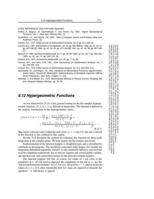
6.12Hypergeometric Functions 271Sample page from NUMERICAL RECIPES IN C: THE ART OF SCIENTIFIC COMPUTING (ISBN 0-521-43108-5)Copyright (C) 1988-1992 by Cambridge University Press.Programs Copyright (C) 1988-1992 by Numerical Recipes Software. Permission is granted for internet users to make one paper copy for their own personal use. Further reproduction, or any copying of machine-readable files (including this one) to any server computer, is strictly prohibited. To order Numerical Recipes books or CDROMs, visit website or call 1-800-872-7423 (North America only),or send email to directcustserv@ (outside North America).CITED REFERENCES AND FURTHER READING:Erd´elyi,A.,Magnus,W.,Oberhettinger,F .,and T ricomi,F .G.1953,Higher T ranscendentalFunctions ,Vol.II,(New Y ork:McGraw-Hill).[1]Gradshteyn,I.S.,and Ryzhik,I.W.1980,T able of Integrals,Series,and Products (New Y ork:Academic Press).[2]Carlson,B.C.1977,SIAM Journal on Mathematical Analysis ,vol.8,pp.231–242.[3]Carlson,B.C.1987,Mathematics of Computation ,vol.49,pp.595–606[4];1988,op.cit.,vol.51,pp.267–280[5];1989,op.cit.,vol.53,pp.327–333[6];1991,op.cit.,vol.56,pp.267–280.[7]Bulirsch,R.1965,Numerische Mathematik ,vol.7,pp.78–90;1965,op.cit.,vol.7,pp.353–354;1969,op.cit.,vol.13,pp.305–315.[8]Carlson,B.C.1979,Numerische Mathematik ,vol.33,pp.1–16.[9]Carlson,B.C.,and Notis,E.M.1981,ACM T ransactions on Mathematical Software ,vol.7,pp.398–403.[10]Carlson,B.C.1978,SIAM Journal on Mathematical Analysis ,vol.9,p.524–528.[11]Abramowitz,M.,and Stegun,I.A.1964,Handbook of Mathematical Functions ,Applied Mathe-matics Series,Volume 55(Washington:National Bureau of Standards;reprinted 1968by Dover Publications,New Y ork),Chapter 17.[12]Mathews,J.,and Walker,R.L.1970,Mathematical Methods of Physics ,2nd ed.(Reading,MA:W.A.Benjamin/Addison-Wesley),pp.78–79.6.12Hypergeometric FunctionsAs was discussed in §5.14,a fast,general routine for the the complex hyperge-ometric function 2F 1(a,b,c ;z ),is difficult or impossible.The function is defined as the analytic continuation of the hypergeometric series,2F 1(a,b,c ;z )=1+ab c z 1!+a (a +1)b (b +1)c (c +1)z 22!+···+a (a +1)...(a +j −1)b (b +1)...(b +j −1)z j+···(6.12.1)This series converges only within the unit circle |z |<1(see [1]),but one’s interest in the function is not confined to this region.Section 5.14discussed the method of evaluating this function by direct path integration in the complex plane.We here merely list the routines that result.Implementation of the function hypgeo is straightforward,and is described by comments in the program.The machinery associated with Chapter 16’s routine for integrating differential equations,odeint ,is only minimally intrusive,and need not even be completely understood:use of odeint requires one zeroed global variable,one function call,and a prescribed format for the derivative routine hypdrv .The function hypgeo will fail,of course,for values of z too close to the singularity at 1.(If you need to approach this singularity,or the one at ∞,use the “linear transformation formulas”in §15.3of [1].)Away from z =1,and for moderate values of a,b,c ,it is often remarkable how few steps are required to integrate the equations.A half-dozen is typical.272Chapter 6.Special FunctionsSample page from NUMERICAL RECIPES IN C: THE ART OF SCIENTIFIC COMPUTING (ISBN 0-521-43108-5)Copyright (C) 1988-1992 by Cambridge University Press.Programs Copyright (C) 1988-1992 by Numerical Recipes Software. Permission is granted for internet users to make one paper copy for their own personal use. Further reproduction, or any copying of machine-readable files (including this one) to any server computer, is strictly prohibited. To order Numerical Recipes books or CDROMs, visit website or call 1-800-872-7423 (North America only),or send email to directcustserv@ (outside North America).#include <math.h>#include "complex.h"#include "nrutil.h"#define EPS 1.0e-6Accuracy parameter.fcomplex aa,bb,cc,z0,dz;Communicates with hypdrv .int kmax,kount;Used by odeint .float *xp,**yp,dxsav;fcomplex hypgeo(fcomplex a,fcomplex b,fcomplex c,fcomplex z)Complex hypergeometric function 2F 1for complex a,b,c ,and z ,by direct integration of the hypergeometric equation in the complex plane.The branch cut is taken to lie along the real axis,Re z >1.{void bsstep(float y[],float dydx[],int nv,float *xx,float htry,float eps,float yscal[],float *hdid,float *hnext,void (*derivs)(float,float [],float []));void hypdrv(float s,float yy[],float dyyds[]);void hypser(fcomplex a,fcomplex b,fcomplex c,fcomplex z,fcomplex *series,fcomplex *deriv);void odeint(float ystart[],int nvar,float x1,float x2,float eps,float h1,float hmin,int *nok,int *nbad,void (*derivs)(float,float [],float []),void (*rkqs)(float [],float [],int,float *,float,float,float [],float *,float *,void (*)(float,float [],float [])));int nbad,nok;fcomplex ans,y[3];float *yy;kmax=0;if (z.r*z.r+z.i*z.i <=0.25){Use series...hypser(a,b,c,z,&ans,&y[2]);return ans;}else if (z.r <0.0)z0=Complex(-0.5,0.0);...or pick a starting point for the path integration.else if (z.r <=1.0)z0=Complex(0.5,0.0);else z0=Complex(0.0,z.i >=0.0?0.5:-0.5);aa=a;Load the global variables to pass pa-rameters “over the head”of odeint to hypdrv .bb=b;cc=c;dz=Csub(z,z0);hypser(aa,bb,cc,z0,&y[1],&y[2]);Get starting function and derivative.yy=vector(1,4);yy[1]=y[1].r;yy[2]=y[1].i;yy[3]=y[2].r;yy[4]=y[2].i;odeint(yy,4,0.0,1.0,EPS,0.1,0.0001,&nok,&nbad,hypdrv,bsstep);The arguments to odeint are the vector of independent variables,its length,the starting and ending values of the dependent variable,the accuracy parameter,an initial guess for stepsize,a minimum stepsize,the (returned)number of good and bad steps taken,and the names of the derivative routine and the (here Bulirsch-Stoer)stepping routine.y[1]=Complex(yy[1],yy[2]);free_vector(yy,1,4);return y[1];}6.12Hypergeometric Functions 273Sample page from NUMERICAL RECIPES IN C: THE ART OF SCIENTIFIC COMPUTING (ISBN 0-521-43108-5)Copyright (C) 1988-1992 by Cambridge University Press.Programs Copyright (C) 1988-1992 by Numerical Recipes Software. Permission is granted for internet users to make one paper copy for their own personal use. Further reproduction, or any copying of machine-readable files (including this one) to any server computer, is strictly prohibited. To order Numerical Recipes books or CDROMs, visit website or call 1-800-872-7423 (North America only),or send email to directcustserv@ (outside North America).#include "complex.h"#define ONE Complex(1.0,0.0)void hypser(fcomplex a,fcomplex b,fcomplex c,fcomplex z,fcomplex *series,fcomplex *deriv)Returns the hypergeometric series 2F 1and its derivative,iterating to machine accuracy.For |z |≤1/2convergence is quite rapid.{void nrerror(char error_text[]);int n;fcomplex aa,bb,cc,fac,temp;deriv->r=0.0;deriv->i=0.0;fac=Complex(1.0,0.0);temp=fac;aa=a;bb=b;cc=c;for (n=1;n<=1000;n++){fac=Cmul(fac,Cdiv(Cmul(aa,bb),cc));deriv->r+=fac.r;deriv->i+=fac.i;fac=Cmul(fac,RCmul(1.0/n,z));*series=Cadd(temp,fac);if (series->r ==temp.r &&series->i ==temp.i)return;temp=*series;aa=Cadd(aa,ONE);bb=Cadd(bb,ONE);cc=Cadd(cc,ONE);}nrerror("convergence failure in hypser");}#include "complex.h"#define ONE Complex(1.0,0.0)extern fcomplex aa,bb,cc,z0,dz;Defined in hypgeo .void hypdrv(float s,float yy[],float dyyds[])Computes derivatives for the hypergeometric equation,see text equation (5.14.4).{fcomplex z,y[3],dyds[3];y[1]=Complex(yy[1],yy[2]);y[2]=Complex(yy[3],yy[4]);z=Cadd(z0,RCmul(s,dz));dyds[1]=Cmul(y[2],dz);dyds[2]=Cmul(Csub(Cmul(Cmul(aa,bb),y[1]),Cmul(Csub(cc,Cmul(Cadd(Cadd(aa,bb),ONE),z)),y[2])),Cdiv(dz,Cmul(z,Csub(ONE,z))));dyyds[1]=dyds[1].r;dyyds[2]=dyds[1].i;dyyds[3]=dyds[2].r;dyyds[4]=dyds[2].i;}CITED REFERENCES AND FURTHER READING:Abramowitz,M.,and Stegun,I.A.1964,Handbook of Mathematical Functions ,Applied Mathe-matics Series,Volume 55(Washington:National Bureau of Standards;reprinted 1968by Dover Publications,New Y ork).[1]。
维生素C的测定实验报告
2.指出本实验采用的定量测定维生素C的方法有何优缺点?
答:优点:2,6-二氯靛酚(DCIP)滴定法利用还原型VC能将染料DCIP还原
为无色的原理,有经济、准确、快速、简便的特点,常用于果蔬中还原型VC含量测定。
缺点:该方法是利用DCIP染料滴定果蔬提取液,只能测定还原型抗坏血酸,不能测出具有同样生理功能的氧化型抗坏血酸和结合型抗坏血酸。滴定终点为过量一滴染料呈现的红色,所以待测果蔬呈红色,提取液本身颜色会干扰滴定终点的观察。
维生素C的应用:胶原蛋白的合成;治疗坏血病;预防牙龈萎缩、出血;预防动脉硬化;抗氧化剂;治疗贫血;防癌;保护作用;提高人体的免疫力;提高机体的应急能力。
4.为何整个滴定过程不要超过2分钟?
答:因为还原型抗坏血酸易被氧化,空气中的氧气会氧化Vc,样品中没有抗氧化的2%的草酸Vc就更容易被氧化,所以滴定过程不要超过2分钟。
教师批阅评语:
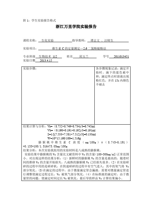
S=1/[(7.533+7.581+7.512)/3]=0.133ml
W=10*15.160/100=1.516g
猕猴桃中维生素C浓度(mg/100g)=(8.745-0,191)*0.133*100/1.516=75.05mg/100g
结果分析:本次实验我组用的实验材料是八成熟的猕猴桃。
实验结果中猕猴桃的Vc含量比文献资料中Vc的含量(100-300mg/ml)正常范围小。对出现这样的结果分析:(1)新鲜时的猕猴桃Vc的含量是最高的,随着时间的推移Vc的含量开始损失,八成熟的猕猴桃Vc已经损失很多。(2)在实验研碎的过程中用的是研碎机,在快速研碎的过程中有空气进入,其中的氧气将Vc部分氧化。(3)在滴定的过程中,由于微量滴定管会漏液,需要对微量滴定管进行调整使滴定过程过长,Vc被氧气部分氧化。(4)在标准液的滴定时,由于微量管的问题,使滴定时间过长Vc被氧化,最后导致样品Vc计算结果偏小。
数值分析课后习题答案
习 题 一 解 答1.取3.14,3.15,227,355113作为π的近似值,求各自的绝对误差,相对误差和有效数字的位数。
分析:求绝对误差的方法是按定义直接计算。
求相对误差的一般方法是先求出绝对误差再按定义式计算。
注意,不应先求相对误差再求绝对误差。
有效数字位数可以根据定义来求,即先由绝对误差确定近似数的绝对误差不超过那一位的半个单位,再确定有效数的末位是哪一位,进一步确定有效数字和有效数位。
有了定理2后,可以根据定理2更规范地解答。
根据定理2,首先要将数值转化为科学记数形式,然后解答。
解:(1)绝对误差:e(x)=π-3.14=3.14159265…-3.14=0.00159…≈0.0016。
相对误差:3()0.0016()0.51103.14r e x e x x -==≈⨯有效数字:因为π=3.14159265…=0.314159265…×10,3.14=0.314×10,m=1。
而π-3.14=3.14159265…-3.14=0.00159…所以│π-3.14│=0.00159…≤0.005=0.5×10-2=21311101022--⨯=⨯所以,3.14作为π的近似值有3个有效数字。
(2)绝对误差:e(x)=π-3.15=3.14159265…-3.14=-0.008407…≈-0.0085。
相对误差:2()0.0085()0.27103.15r e x e x x --==≈-⨯有效数字:因为π=3.14159265…=0.314159265…×10,3.15=0.315×10,m=1。
而π-3.15=3.14159265…-3.15=-0.008407…所以│π-3.15│=0.008407……≤0.05=0.5×10-1=11211101022--⨯=⨯所以,3.15作为π的近似值有2个有效数字。
(3)绝对误差:22() 3.141592653.1428571430.0012644930.00137e x π=-=-=-≈-相对误差:3()0.0013()0.4110227r e x e x x--==≈-⨯有效数字: 因为π=3.14159265…=0.314159265…×10, 223.1428571430.3142857143107==⨯,m=1。
c-8位甲氧基 -回复
c-8位甲氧基-回复【c8位甲氧基】化合物及其应用引言:化学合成领域中,功能性基团的引入对于设计和合成具有特定性质的化合物具有重要意义。
其中的一个重要功能基团就是甲氧基(methoxy,–OCH3)基团,它包含一个碳-氧键以及一个甲基基团。
在碳骨架上的不同位置引入甲氧基,可以产生多种不同的化合物,其中包括c8位甲氧基的化合物。
本文将从c8位甲氧基的定义、合成方法和应用方面进行阐述。
一、c8位甲氧基的定义c8位甲氧基是指将甲氧基基团引入到分子的第8个碳原子上。
在有机化学中,通常使用数字来标记碳原子的位置。
对于具有连续碳骨架的有机化合物,可以用数字来标记每个碳原子的位置,从而辨别不同的位点。
因此,c8位甲氧基表示甲氧基基团连接在分子的第8个碳原子上。
二、c8位甲氧基的合成方法1. 核苷化合物工具:核苷化合物是常用的合成c8位甲氧基的起始材料之一。
核苷化合物是由糖类和碱基两部分组成的,可以通过差异化修饰糖部分来引入甲氧基基团。
例如,通过保护糖部分的羟基,然后在c8位引入甲氧基,最后再去除保护基团,得到c8位甲氧基的核苷化合物。
2. 置换反应:另一种常用的合成c8位甲氧基的方法是通过置换反应。
这种方法通常涉及到通过亲核取代反应,用带有甲氧基的试剂替代分子中原有的官能团。
例如,可以使用类似碘甲烷等试剂,在碳原子的位置将碘原子置换为甲氧基基团。
3. 氧化反应:氧化反应也可以用于合成c8位甲氧基的化合物。
例如,可以使用过氧化物或者氧化剂来将分子中的碳原子转变成碳氧化合物,进而引入甲氧基基团。
三、c8位甲氧基的应用1. 药物合成:c8位甲氧基的化合物在药物领域具有广泛的应用。
该功能基团可以改变药物的物理化学性质,例如溶解度、稳定性和生物活性。
一些研究表明,引入c8位甲氧基的药物分子往往具有更好的生物利用度和药效。
2. 化学合成:c8位甲氧基也被广泛用于有机合成中。
在合成复杂有机化合物时,可以利用c8位甲氧基作为反应步骤的保护基团,以避免其他官能团的干扰。
EXP8Vc含量测定
►从滴定时2,6- 二氯酚靛 酚标淮溶液的消耗量,可 以计算出被检物质中VC 的含量
►氧化型的2,6-二氯酚靛酚在酸性 溶液中呈红色
3.试剂&材料&仪器
标准抗坏血酸溶液(1mg/mL): 准确称取100mg纯 抗坏血酸(应为洁白色,如变为黄色则不能用)溶于 1%草酸溶液中,并稀释至100mL,贮于棕色瓶中, 冷藏。最好临用前配制。
称取10-30g 加入20mL 2%草酸
研磨
静置约10min 2层纱布过滤
滤液(如浑浊可离心)滤入50mL容量瓶
反复抽提2~3次 用 2%草酸
将滤液并入同一容量瓶中 定容
混匀
计算
提取液10mL于锥形瓶
空白对照Βιβλιοθήκη 重复2-3次 滴定整个滴定过程不要超过2min
微弱的玫瑰色 终点
标准液滴定
准确吸取标准抗坏血酸溶液1mL置50mL锥形瓶中,加 9mL 1%草酸,用微量滴定管以0.1% 2,6-二氯酚靛 酚溶液滴定至淡红色,并保持15s不褪色,即达终点。 由所用染料的体积计算出1mL染料相当于多少mg抗坏 血酸(取10mL 1%草酸作空白对照,按以上方法滴 定)。
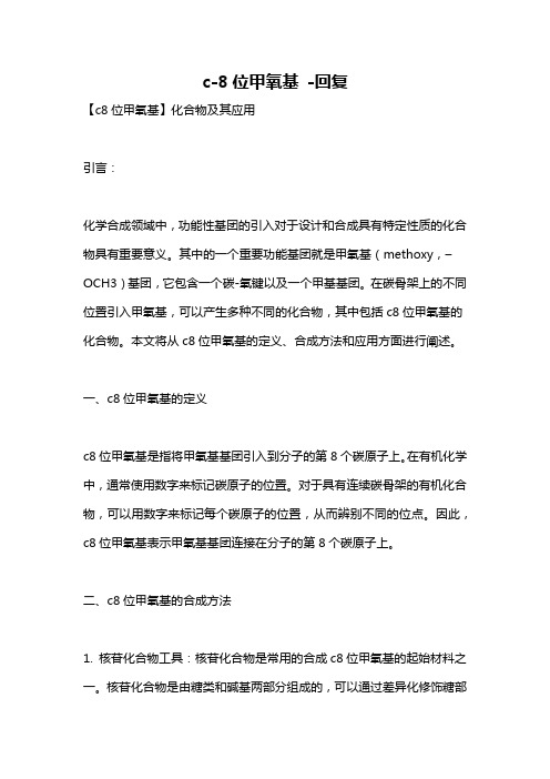
▪ VC在机体内参与氧化还原反应,是一些氧化还原酶的辅酶,能 保护机体中许多含—SH基的酶使之不受氧化;
▪ VC在体内能促进胶原蛋白和粘多糖的合成,增加微血管的致密 性,降低其通透性及脆性
▪VC促进免疫球蛋白的合成,增强 机体的抵抗力; ▪VC有增强机体对肿瘤的抵抗力, 并具有对化学致癌物的阻断作用; ▪VC能使氧化型谷光甘肽转化为还 原 型 谷 光 甘 肽 ( 简 称 GSH ) , 而 GSH可与重金属结合而排出体外, 因此VC常用于重金属的解毒。
c6仪器原理

c6仪器原理
C6仪器原理
C6仪器是一种用于测量样品中的碳、氮、硫、氧等元素含量的仪器。
它采用了现代化的技术,可以高效、准确地分析样品中的元素含量,具有广泛的应用价值。
C6仪器的工作原理是基于元素分析的原理。
在样品中,元素存在于化合物的形式下,因此需要将其分解为单质状态,才能进行分析。
C6仪器采用了高温燃烧-红外检测的方法,将样品中的化合物分解为单质状态,然后通过红外检测器检测单质的含量,从而计算出样品中元素的含量。
具体来说,C6仪器的工作流程如下:
1. 样品处理
样品首先需要进行处理,以去除样品中的杂质和水分等物质。
通常情况下,样品需要经过研磨、筛选、干燥等步骤,以确保样品的纯度和均匀度。
2. 燃烧
处理后的样品被放入燃烧器中,加热至高温状态。
在高温状态下,样品中的化合物会被分解为单质状态,如硫化物会被分解成SO2和H2O,氧化物会被分解成CO2和H2O等。
3. 红外检测
分解后的单质进入红外检测器,利用红外吸收光谱的原理,检测单质的含量。
红外吸收光谱是一种非常敏感的检测方法,可以检测出极低浓度的单质,从而保证分析结果的准确性。
4. 计算元素含量
根据红外检测器检测到的单质含量,计算出样品中元素的含量。
计算过程中需要考虑多种因素,如样品中其他元素的影响、红外检测器的响应特性等,以确保分析结果的准确性。
C6仪器的优点是分析速度快、准确性高、操作简便等。
同时,C6仪器还可以进行多种元素的分析,如碳、氮、硫、氧等元素,具有广泛的应用价值。
在化学、环境、食品等领域,C6仪器已经成为一种不可或缺的分析工具。
分子荧光法测定维生素C 的含量

注意事项
• 生成的荧光物质见光易分解,实验过程要注意避 光。
• 维生素C(抗坏血酸)在1%草酸溶剂中,可被2,6二氯酚靛酚定量氧化成脱氢抗坏血酸,与邻苯二 胺(OPDA)反应生成蓝色荧光物质,用荧光分光光 度计测定其荧光强度,其荧光强度与维生素C的浓 度成正比,以外标法定量。
• 试样中可能存在的丙酮酸与OPDA反应,生成荧光 化合物,脱氢抗坏血酸与硼酸可形成复合物不与 邻苯二胺反应,硼酸不与丙酮酸作用,由此可以 排除试样中荧光杂质产生的干扰。
• 荧光是物质吸收光的能量后产生的,因此任何荧光物 质都具有两种光谱:激发光谱和发射光谱。不同物质 由于分子结构的不同,其激发态能级的分布具有各自 不同的特征,这种特征反映在荧光上表现为各种物质 都有其特征荧光激发和发射光谱,因此可以用荧光激 发和发射光谱的不同来定性地进行物质的鉴定。
• 荧光强度是表示发射相对强度的物理量,它是最常用的荧 光参数之一。目前一般的商品仪器都采用荧光强度来表示, 所以单位为任意单位,表示的是相对强度。物质发射的荧 光强度与它吸收的光能成正比,当测量的溶液很稀时,可 用如下公式表示:
实验步骤
• 1.工作曲线的绘制 • 取50ml棕色容量瓶8只,分别加入100mg/l抗坏血酸标准溶
液0.10,0.40,0.80,1.60ml各两份;各逐滴加入0.1% 2,6二氯酚靛酚溶液至样品溶液显微红色,再加入硫脲使红色 退去,再向一系列中加入2ml硼酸-乙酸钠溶液(空白系 列),另一系列中加入2ml乙酸钠溶液,在避光条件下不 断振摇15min;各加入0.2g/L邻苯二胺6ml,摇匀,于暗处放 置40-45min,用1%草酸溶液定容至刻度,然后以365nm光 激发,在429处测量荧光强度,以荧光强度(扣除空白) 为纵坐标,以浓度为横坐标作工作曲线。 • 2.待测试样的测定 • 与步骤1同时进行,取未知样品按上述程序操作并测量荧 光强度,平行测定两份,从工作曲线上查的待测液浓度并 计算待测样中维生素的含量。
c6仪器原理
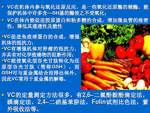
c6仪器原理C6仪器原理C6仪器是一种用于分析和检测材料成分的仪器,其原理基于光谱技术。
光谱技术是通过测量材料与特定波长的光的相互作用来获取关于材料成分的信息的一种方法。
C6仪器使用的光谱技术主要有紫外-可见光吸收光谱和红外光谱。
紫外-可见光吸收光谱是通过测量材料对紫外-可见光的吸收来确定材料的成分。
红外光谱则是通过测量材料对红外光的吸收或散射来获得材料成分的信息。
C6仪器的工作原理可以简单概括为以下几个步骤:1. 光源发射:C6仪器通过一个光源发射特定波长的光,这些波长的选择取决于所要分析的材料成分。
2. 光与样品的相互作用:发射的光通过一个样品池或探头与待分析的样品相互作用。
在这个过程中,光会被样品吸收、散射或透射。
3. 光谱的获取:C6仪器会测量经过样品后的光的强度和波长变化。
根据光的强度和波长的变化,可以得到样品对不同波长光的吸收或散射的信息。
4. 数据处理:C6仪器会将测量得到的光谱数据进行处理和分析。
通过与已知标准样品进行比较,可以确定样品中的成分。
C6仪器的原理可以应用于多种领域,如化学、生物、环境监测等。
在化学领域,C6仪器可以用于分析溶液中的化学物质浓度。
在生物领域,C6仪器可以用于分析生物样品中的蛋白质、核酸等分子的含量。
在环境监测领域,C6仪器可以用于检测空气中的污染物浓度。
C6仪器的优点在于其快速、准确和无损的分析方法。
相比传统的化学分析方法,C6仪器可以在短时间内完成分析,并且不需要破坏样品。
此外,C6仪器还可以进行实时监测,对于需要频繁分析的应用场景非常适用。
然而,C6仪器也有一些限制。
首先,C6仪器对样品的要求比较高,需要样品具备一定的透明性或散射性。
其次,C6仪器在分析复杂样品时可能存在干扰,需要进行数据处理和校正。
总的来说,C6仪器是一种基于光谱技术的分析仪器,通过测量样品与特定波长光的相互作用来获得样品的成分信息。
它具有快速、准确和无损的特点,在化学、生物、环境监测等领域有着广泛的应用前景。
- 1、下载文档前请自行甄别文档内容的完整性,平台不提供额外的编辑、内容补充、找答案等附加服务。
- 2、"仅部分预览"的文档,不可在线预览部分如存在完整性等问题,可反馈申请退款(可完整预览的文档不适用该条件!)。
- 3、如文档侵犯您的权益,请联系客服反馈,我们会尽快为您处理(人工客服工作时间:9:00-18:30)。
252Chapter 6.Special FunctionsSample page from NUMERICAL RECIPES IN C: THE ART OF SCIENTIFIC COMPUTING (ISBN 0-521-43108-5)Copyright (C) 1988-1992 by Cambridge University Press.Programs Copyright (C) 1988-1992 by Numerical Recipes Software. Permission is granted for internet users to make one paper copy for their own personal use. Further reproduction, or any copying of machine-readable files (including this one) to any server computer, is strictly prohibited. To order Numerical Recipes books or CDROMs, visit website or call 1-800-872-7423 (North America only),or send email to directcustserv@ (outside North America).CITED REFERENCES AND FURTHER READING:Barnett,A.R.,Feng,D.H.,Steed,J.W.,and Goldfarb,L.J.B.1974,Computer Physics Commu-nications ,vol.8,pp.377–395.[1]T emme,N.M.1976,Journal of Computational Physics ,vol.21,pp.343–350[2];1975,op.cit.,vol.19,pp.324–337.[3]Thompson,I.J.,and Barnett,A.R.1987,Computer Physics Communications ,vol.47,pp.245–257.[4]Barnett,A.R.1981,Computer Physics Communications ,vol.21,pp.297–314.Thompson,I.J.,and Barnett,A.R.1986,Journal of Computational Physics ,vol.64,pp.490–509.Abramowitz,M.,and Stegun,I.A.1964,Handbook of Mathematical Functions ,Applied Mathe-matics Series,Volume 55(Washington:National Bureau of Standards;reprinted 1968by Dover Publications,New Y ork),Chapter 10.6.8Spherical HarmonicsSpherical harmonics occur in a large variety of physical problems,for ex-ample,whenever a wave equation,or Laplace’s equation,is solved by separa-tion of variables in spherical coordinates.The spherical harmonic Y lm (θ,φ),−l ≤m ≤l,is a function of the two coordinates θ,φon the surface of a sphere.The spherical harmonics are orthogonal for different l and m ,and they are normalized so that their integrated square over the sphere is unity:2π0dφ1−1d (cos θ)Y l m *(θ,φ)Y lm (θ,φ)=δl l δm m (6.8.1)Here asterisk denotes complex conjugation.Mathematically,the spherical harmonics are related to associated Legendre polynomials by the equationY lm (θ,φ)=2l +14π(l −m )!(l +m )!P ml (cos θ)e imφ(6.8.2)By using the relationY l,−m (θ,φ)=(−1)m Y lm *(θ,φ)(6.8.3)we can always relate a spherical harmonic to an associated Legendre polynomial with m ≥0.With x ≡cos θ,these are defined in terms of the ordinary Legendre polynomials (cf.§4.5and §5.5)byP m l (x )=(−1)m(1−x 2)m/2d mdx mP l (x )(6.8.4)6.8Spherical Harmonics 253Sample page from NUMERICAL RECIPES IN C: THE ART OF SCIENTIFIC COMPUTING (ISBN 0-521-43108-5)Copyright (C) 1988-1992 by Cambridge University Press.Programs Copyright (C) 1988-1992 by Numerical Recipes Software. Permission is granted for internet users to make one paper copy for their own personal use. Further reproduction, or any copying of machine-readable files (including this one) to any server computer, is strictly prohibited. To order Numerical Recipes books or CDROMs, visit website or call 1-800-872-7423 (North America only),or send email to directcustserv@ (outside North America).The first few associated Legendre polynomials,and their corresponding nor-malized spherical harmonics,areP 00(x )=1Y 00= 14πP 11(x )=−(1−x 2)1/2Y 11=−38πsin θe iφP 01(x )=x Y 10=34πcos θP 22(x )=3(1−x 2)Y 22=14152πsin 2θe 2iφP 12(x )=−3(1−x 2)1/2x Y 21=−158πsin θcos θe iφP 02(x )=12(3x 2−1)Y 20=54π(32cos 2θ−12)(6.8.5)There are many bad ways to evaluate associated Legendre polynomials numer-ically.For example,there are explicit expressions,such asP m l (x )=(−1)m (l +m )!2m m !(l −m )!(1−x 2)m/21−(l −m )(m +l +1)1!(m +1) 1−x 2+(l −m )(l −m −1)(m +l +1)(m +l +2) 1−x2−··· (6.8.6)where the polynomial continues up through the term in (1−x )l −m .(See [1]forthis and related formulas.)This is not a satisfactory method because evaluation of the polynomial involves delicate cancellations between successive terms,which alternate in sign.For large l ,the individual terms in the polynomial become very much larger than their sum,and all accuracy is lost.In practice,(6.8.6)can be used only in single precision (32-bit)for l up to 6or 8,and in double precision (64-bit)for l up to 15or 18,depending on the precision required for the answer.A more robust computational procedure is therefore desirable,as follows:The associated Legendre functions satisfy numerous recurrence relations,tab-ulated in [1-2].These are recurrences on l alone,on m alone,and on both l and m simultaneously.Most of the recurrences involving m are unstable,and so dangerous for numerical work.The following recurrence on l is,however,stable (compare 5.5.1):(l −m )P m l =x (2l −1)P m l −1−(l +m −1)P ml −2(6.8.7)It is useful because there is a closed-form expression for the starting value,P m m =(−1)m (2m −1)!!(1−x 2)m/2(6.8.8)(The notation n !!denotes the product of all odd integers less than or equal to n .)Using (6.8.7)with l =m +1,and setting P mm −1=0,we findP m m +1=x (2m +1)P mm(6.8.9)Equations (6.8.8)and (6.8.9)provide the two starting values required for (6.8.7)for general l .The function that implements this is254Chapter 6.Special FunctionsSample page from NUMERICAL RECIPES IN C: THE ART OF SCIENTIFIC COMPUTING (ISBN 0-521-43108-5)Copyright (C) 1988-1992 by Cambridge University Press.Programs Copyright (C) 1988-1992 by Numerical Recipes Software. Permission is granted for internet users to make one paper copy for their own personal use. Further reproduction, or any copying of machine-readable files (including this one) to any server computer, is strictly prohibited. To order Numerical Recipes books or CDROMs, visit website or call 1-800-872-7423 (North America only),or send email to directcustserv@ (outside North America).#include <math.h>float plgndr(int l,int m,float x)Computes the associated Legendre polynomial P m l (x ).Here m and l are integers satisfying 0≤m ≤l ,while x lies in the range −1≤x ≤1.{void nrerror(char error_text[]);float fact,pll,pmm,pmmp1,somx2;int i,ll;if (m <0||m >l ||fabs(x)>1.0)nrerror("Bad arguments in routine plgndr");pmm=1.0;Compute P m m.if (m >0){somx2=sqrt((1.0-x)*(1.0+x));fact=1.0;for (i=1;i<=m;i++){pmm *=-fact*somx2;fact +=2.0;}}if (l ==m)return pmm;else {Compute P m m +1.pmmp1=x*(2*m+1)*pmm;if (l ==(m+1))return pmmp1;else {Compute P m l ,l >m +1.for (ll=m+2;ll<=l;ll++){pll=(x*(2*ll-1)*pmmp1-(ll+m-1)*pmm)/(ll-m);pmm=pmmp1;pmmp1=pll;}return pll;}}}CITED REFERENCES AND FURTHER READING:Magnus,W.,and Oberhettinger,F .1949,Formulas and Theorems for the Functions of Mathe-matical Physics (New Y ork:Chelsea),pp.54ff.[1]Abramowitz,M.,and Stegun,I.A.1964,Handbook of Mathematical Functions ,Applied Mathe-matics Series,Volume 55(Washington:National Bureau of Standards;reprinted 1968by Dover Publications,New Y ork),Chapter 8.[2]6.9Fresnel Integrals,Cosine and Sine Integrals 255Sample page from NUMERICAL RECIPES IN C: THE ART OF SCIENTIFIC COMPUTING (ISBN 0-521-43108-5)Copyright (C) 1988-1992 by Cambridge University Press.Programs Copyright (C) 1988-1992 by Numerical Recipes Software. Permission is granted for internet users to make one paper copy for their own personal use. Further reproduction, or any copying of machine-readable files (including this one) to any server computer, is strictly prohibited. To order Numerical Recipes books or CDROMs, visit website or call 1-800-872-7423 (North America only),or send email to directcustserv@ (outside North America).6.9Fresnel Integrals,Cosine and Sine IntegralsFresnel IntegralsThe two Fresnel integrals are defined byC (x )=x0cos π2t 2 dt,S (x )=xsin π2t 2 dt (6.9.1)The most convenient way of evaluating these functions to arbitrary precision is to use power series for small x and a continued fraction for large x .The series areC (x )=x − π2 2x 55·2!+ π2 4x 99·4!−···S (x )= π2 x 33·1!− π2 3x 77·3!+ π2 5x 1111·5!−···(6.9.2)There is a complex continued fraction that yields both S (x )and C (x )simul-taneously:C (x )+iS (x )=1+i 2erf z,z =√π2(1−i )x (6.9.3)wheree z2erfc z =1√π1z +1/2z +1z +3/2z +2z +··· =2z √π11·23·4···(6.9.4)In the last line we have converted the “standard”form of the continued fraction to its “even”form (see §5.2),which converges twice as fast.We must be careful not to evaluate the alternating series (6.9.2)at too large a value of x ;inspection of the terms shows that x =1.5is a good point to switch over to the continued fraction.Note that for large xC (x )∼12+1πx sin π2x 2 ,S (x )∼12−1πx cos π2x 2(6.9.5)Thus the precision of the routine frenel may be limited by the precision of thelibrary routines for sine and cosine for large x .。