Princ.econs -lec 12

合集下载

源自欧夏至草的成分的化妆品用途[发明专利]

专利名称：源自欧夏至草的成分的化妆品用途专利类型：发明专利
发明人：C·林根巴赫,E·多瑞多特,P·蒙东
申请号：CN201780015321.0
申请日：20170321
公开号：CN108778242A
公开日：
20181109
专利内容由知识产权出版社提供
摘要：本发明提出了源自欧夏至草(Marrubium vulgare)的植物材料用于紧致皮肤毛孔的非治疗性美容处理的用途，所述植物材料包含有效量的连翘酯苷B作为活性分子。

所述植物材料优选由去除了细胞碎片的去分化植物细胞的细胞提取物组成。

这种治疗特别打算用于细化皮肤纹理和/或用于处理具有油性趋势的皮肤。

申请人：赛德玛公司
地址：法国勒佩雷-恩-伊林斯
国籍：FR
代理机构：中国国际贸易促进委员会专利商标事务所
代理人：李瑛
更多信息请下载全文后查看。

羟基酪醇对H2O2损伤的神经细胞株PC12凋亡影响及其机制

山东医药２０１７年第５７卷第４３期
羟基酪醇对Ｈ２Ｏ２损伤的神经细胞株ＰＣ１２
凋亡影响及其机制
刘旭东，李静，柳太云
（１遵义市第一人民医院，贵州遵义５６３０００；２贵州省人民医院）
活性氧簇（ＲＯＳ）是氧分子的部分还原代谢产
作用，例如，从喂养羟基酪醇的小鼠的脑组织中发现乳酸脱氢酶（ＬＤＡ）呈羟基酪醇剂量依赖性降低，表明羟基酪醇对啮齿动物神经具有保护作用Ｊ。此外，羟基酪醇可显著减轻过氧化氢（Ｈ：Ｏ：）诱导的人神经母细胞瘤细胞的ＤＮＡ损伤。２０１５年５月１１３—２０１７年３月３０日，我们观察了羟基酪醇对Ｈ０：损伤的神经细胞株ＰＣ１２凋亡的影响，并对其
作用机制进行了探讨。现将结果报告如下。
１材料与方法
物的总称，具有很高的生物活性，作为第二信使，它们在多种细胞因子生物活性的启动过程中发挥着重要的作用，参与调节细胞的增殖、分化和凋亡¨ Ｉ２ｊ。
酸脱氢酶（ＬＤＨ）和ＲＯＳ，Ｈｏｅｃｈｓｔ３３２５８荧光染色法测算细胞凋亡率，实时荧光定量ＰＣＲ检测各组细胞Ｂａｘ、Ｂｃｌ－２、
Ｃａｓｐａｓｅ－３ｍＲＮＡ，免疫印迹试验检测各组ＮＦ — ＫＢ、ｐ — ＮＦ — ＫＢＳｅｒ５３６蛋白，酶联免疫吸附测定法测定各组ＩＬ — ｌＢ和ＴＮＦ一０【。结果与对照组相比，ＨＯ２组细胞存活率降低（Ｐ＜０．０５）、细胞凋亡率上升（Ｐ＜０．０５）；与Ｈ：Ｏ组相比，观察组细胞存活率上升（Ｐ＜０．０５）、细胞凋亡率降低（Ｐ＜０．０５）。与对照组相比，Ｈ：Ｏ组ＬＤＨ释放率和ＲＯＳ水平升高（Ｐ均＜０．０５）；与ＨＯ２组相比，观察组ＬＤＨ释放率和ＲＯＳ水平降低（Ｐ均＜０．０５）。与对照组相比，ＨＯ组ＢａｘｍＲＮＡ相对表达量升高（Ｐ＜０．０５）、Ｂｃｌ－２ｍＲＮＡ相对表达量降低（Ｐ＜０．０５）、Ｃａｓｐａｓｅ一３ｍＲＮＡ相对表达量升高（Ｐ＜０．０ＢａｘｍＲＮＡ相对表达量降低（Ｐ＜０．０５）、Ｂｃｌ一２ｍＲＮＡ相对表达量升高（Ｐ＜０．０５）、Ｃａｓｐａｓｅ一３ｍＲＮＡ相对表达量降低（Ｐ＜０．０５）。与对照组相比，Ｈ２Ｏ：组ＮＦ・ＫＢ、ｐ－ＮＦ — ＫＢＳｅｒ５３６蛋白表达量

Multicamera People Tracking with a Probabilistic Occupancy Map

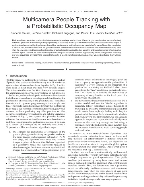
Multicamera People Tracking witha Probabilistic Occupancy MapFranc¸ois Fleuret,Je´roˆme Berclaz,Richard Lengagne,and Pascal Fua,Senior Member,IEEE Abstract—Given two to four synchronized video streams taken at eye level and from different angles,we show that we can effectively combine a generative model with dynamic programming to accurately follow up to six individuals across thousands of frames in spite of significant occlusions and lighting changes.In addition,we also derive metrically accurate trajectories for each of them.Our contribution is twofold.First,we demonstrate that our generative model can effectively handle occlusions in each time frame independently,even when the only data available comes from the output of a simple background subtraction algorithm and when the number of individuals is unknown a priori.Second,we show that multiperson tracking can be reliably achieved by processing individual trajectories separately over long sequences,provided that a reasonable heuristic is used to rank these individuals and that we avoid confusing them with one another.Index Terms—Multipeople tracking,multicamera,visual surveillance,probabilistic occupancy map,dynamic programming,Hidden Markov Model.Ç1I NTRODUCTIONI N this paper,we address the problem of keeping track of people who occlude each other using a small number of synchronized videos such as those depicted in Fig.1,which were taken at head level and from very different angles. This is important because this kind of setup is very common for applications such as video surveillance in public places.To this end,we have developed a mathematical framework that allows us to combine a robust approach to estimating the probabilities of occupancy of the ground plane at individual time steps with dynamic programming to track people over time.This results in a fully automated system that can track up to six people in a room for several minutes by using only four cameras,without producing any false positives or false negatives in spite of severe occlusions and lighting variations. As shown in Fig.2,our system also provides location estimates that are accurate to within a few tens of centimeters, and there is no measurable performance decrease if as many as20percent of the images are lost and only a small one if 30percent are.This involves two algorithmic steps:1.We estimate the probabilities of occupancy of theground plane,given the binary images obtained fromthe input images via background subtraction[7].Atthis stage,the algorithm only takes into accountimages acquired at the same time.Its basic ingredientis a generative model that represents humans assimple rectangles that it uses to create synthetic idealimages that we would observe if people were at givenlocations.Under this model of the images,given thetrue occupancy,we approximate the probabilities ofoccupancy at every location as the marginals of aproduct law minimizing the Kullback-Leibler diver-gence from the“true”conditional posterior distribu-tion.This allows us to evaluate the probabilities ofoccupancy at every location as the fixed point of alarge system of equations.2.We then combine these probabilities with a color and amotion model and use the Viterbi algorithm toaccurately follow individuals across thousands offrames[3].To avoid the combinatorial explosion thatwould result from explicitly dealing with the jointposterior distribution of the locations of individuals ineach frame over a fine discretization,we use a greedyapproach:we process trajectories individually oversequences that are long enough so that using areasonable heuristic to choose the order in which theyare processed is sufficient to avoid confusing peoplewith each other.In contrast to most state-of-the-art algorithms that recursively update estimates from frame to frame and may therefore fail catastrophically if difficult conditions persist over several consecutive frames,our algorithm can handle such situations since it computes the global optima of scores summed over many frames.This is what gives it the robustness that Fig.2demonstrates.In short,we combine a mathematically well-founded generative model that works in each frame individually with a simple approach to global optimization.This yields excellent performance by using basic color and motion models that could be further improved.Our contribution is therefore twofold.First,we demonstrate that a generative model can effectively handle occlusions at each time frame independently,even when the input data is of very poor quality,and is therefore easy to obtain.Second,we show that multiperson tracking can be reliably achieved by processing individual trajectories separately over long sequences.. F.Fleuret,J.Berclaz,and P.Fua are with the Ecole Polytechnique Fe´de´ralede Lausanne,Station14,CH-1015Lausanne,Switzerland.E-mail:{francois.fleuret,jerome.berclaz,pascal.fua}@epfl.ch..R.Lengagne is with GE Security-VisioWave,Route de la Pierre22,1024Ecublens,Switzerland.E-mail:richard.lengagne@.Manuscript received14July2006;revised19Jan.2007;accepted28Mar.2007;published online15May2007.Recommended for acceptance by S.Sclaroff.For information on obtaining reprints of this article,please send e-mail to:tpami@,and reference IEEECS Log Number TPAMI-0521-0706.Digital Object Identifier no.10.1109/TPAMI.2007.1174.0162-8828/08/$25.00ß2008IEEE Published by the IEEE Computer SocietyIn the remainder of the paper,we first briefly review related works.We then formulate our problem as estimat-ing the most probable state of a hidden Markov process and propose a model of the visible signal based on an estimate of an occupancy map in every time frame.Finally,we present our results on several long sequences.2R ELATED W ORKState-of-the-art methods can be divided into monocular and multiview approaches that we briefly review in this section.2.1Monocular ApproachesMonocular approaches rely on the input of a single camera to perform tracking.These methods provide a simple and easy-to-deploy setup but must compensate for the lack of 3D information in a single camera view.2.1.1Blob-Based MethodsMany algorithms rely on binary blobs extracted from single video[10],[5],[11].They combine shape analysis and tracking to locate people and maintain appearance models in order to track them,even in the presence of occlusions.The Bayesian Multiple-BLob tracker(BraMBLe)system[12],for example,is a multiblob tracker that generates a blob-likelihood based on a known background model and appearance models of the tracked people.It then uses a particle filter to implement the tracking for an unknown number of people.Approaches that track in a single view prior to computing correspondences across views extend this approach to multi camera setups.However,we view them as falling into the same category because they do not simultaneously exploit the information from multiple views.In[15],the limits of the field of view of each camera are computed in every other camera from motion information.When a person becomes visible in one camera,the system automatically searches for him in other views where he should be visible.In[4],a background/foreground segmentation is performed on calibrated images,followed by human shape extraction from foreground objects and feature point selection extraction. Feature points are tracked in a single view,and the system switches to another view when the current camera no longer has a good view of the person.2.1.2Color-Based MethodsTracking performance can be significantly increased by taking color into account.As shown in[6],the mean-shift pursuit technique based on a dissimilarity measure of color distributions can accurately track deformable objects in real time and in a monocular context.In[16],the images are segmented pixelwise into different classes,thus modeling people by continuously updated Gaussian mixtures.A standard tracking process is then performed using a Bayesian framework,which helps keep track of people,even when there are occlusions.In such a case,models of persons in front keep being updated, whereas the system stops updating occluded ones,which may cause trouble if their appearances have changed noticeably when they re-emerge.More recently,multiple humans have been simulta-neously detected and tracked in crowded scenes[20]by using Monte-Carlo-based methods to estimate their number and positions.In[23],multiple people are also detected and tracked in front of complex backgrounds by using mixture particle filters guided by people models learned by boosting.In[9],multicue3D object tracking is addressed by combining particle-filter-based Bayesian tracking and detection using learned spatiotemporal shapes.This ap-proach leads to impressive results but requires shape, texture,and image depth information as input.Finally, Smith et al.[25]propose a particle-filtering scheme that relies on Markov chain Monte Carlo(MCMC)optimization to handle entrances and departures.It also introduces a finer modeling of interactions between individuals as a product of pairwise potentials.2.2Multiview ApproachesDespite the effectiveness of such methods,the use of multiple cameras soon becomes necessary when one wishes to accurately detect and track multiple people and compute their precise3D locations in a complex environment. Occlusion handling is facilitated by using two sets of stereo color cameras[14].However,in most approaches that only take a set of2D views as input,occlusion is mainly handled by imposing temporal consistency in terms of a motion model,be it Kalman filtering or more general Markov models.As a result,these approaches may not always be able to recover if the process starts diverging.2.2.1Blob-Based MethodsIn[19],Kalman filtering is applied on3D points obtained by fusing in a least squares sense the image-to-world projections of points belonging to binary blobs.Similarly,in[1],a Kalman filter is used to simultaneously track in2D and3D,and objectFig.1.Images from two indoor and two outdoor multicamera video sequences that we use for our experiments.At each time step,we draw a box around people that we detect and assign to them an ID number that follows them throughout thesequence.Fig.2.Cumulative distributions of the position estimate error on a3,800-frame sequence(see Section6.4.1for details).locations are estimated through trajectory prediction during occlusion.In[8],a best hypothesis and a multiple-hypotheses approaches are compared to find people tracks from 3D locations obtained from foreground binary blobs ex-tracted from multiple calibrated views.In[21],a recursive Bayesian estimation approach is used to deal with occlusions while tracking multiple people in multiview.The algorithm tracks objects located in the intersections of2D visual angles,which are extracted from silhouettes obtained from different fixed views.When occlusion ambiguities occur,multiple occlusion hypotheses are generated,given predicted object states and previous hypotheses,and tested using a branch-and-merge strategy. The proposed framework is implemented using a customized particle filter to represent the distribution of object states.Recently,Morariu and Camps[17]proposed a method based on dimensionality reduction to learn a correspondence between the appearance of pedestrians across several views. This approach is able to cope with the severe occlusion in one view by exploiting the appearance of the same pedestrian on another view and the consistence across views.2.2.2Color-Based MethodsMittal and Davis[18]propose a system that segments,detects, and tracks multiple people in a scene by using a wide-baseline setup of up to16synchronized cameras.Intensity informa-tion is directly used to perform single-view pixel classifica-tion and match similarly labeled regions across views to derive3D people locations.Occlusion analysis is performed in two ways:First,during pixel classification,the computa-tion of prior probabilities takes occlusion into account. Second,evidence is gathered across cameras to compute a presence likelihood map on the ground plane that accounts for the visibility of each ground plane point in each view. Ground plane locations are then tracked over time by using a Kalman filter.In[13],individuals are tracked both in image planes and top view.The2D and3D positions of each individual are computed so as to maximize a joint probability defined as the product of a color-based appearance model and2D and 3D motion models derived from a Kalman filter.2.2.3Occupancy Map MethodsRecent techniques explicitly use a discretized occupancy map into which the objects detected in the camera images are back-projected.In[2],the authors rely on a standard detection of stereo disparities,which increase counters associated to square areas on the ground.A mixture of Gaussians is fitted to the resulting score map to estimate the likely location of individuals.This estimate is combined with a Kallman filter to model the motion.In[26],the occupancy map is computed with a standard visual hull procedure.One originality of the approach is to keep for each resulting connex component an upper and lower bound on the number of objects that it can contain. Based on motion consistency,the bounds on the various components are estimated at a certain time frame based on the bounds of the components at the previous time frame that spatially intersect with it.Although our own method shares many features with these techniques,it differs in two important respects that we will highlight:First,we combine the usual color and motion models with a sophisticated approach based on a generative model to estimating the probabilities of occu-pancy,which explicitly handles complex occlusion interac-tions between detected individuals,as will be discussed in Section5.Second,we rely on dynamic programming to ensure greater stability in challenging situations by simul-taneously handling multiple frames.3P ROBLEM F ORMULATIONOur goal is to track an a priori unknown number of people from a few synchronized video streams taken at head level. In this section,we formulate this problem as one of finding the most probable state of a hidden Markov process,given the set of images acquired at each time step,which we will refer to as a temporal frame.We then briefly outline the computation of the relevant probabilities by using the notations summarized in Tables1and2,which we also use in the following two sections to discuss in more details the actual computation of those probabilities.3.1Computing the Optimal TrajectoriesWe process the video sequences by batches of T¼100frames, each of which includes C images,and we compute the most likely trajectory for each individual.To achieve consistency over successive batches,we only keep the result on the first 10frames and slide our temporal window.This is illustrated in Fig.3.We discretize the visible part of the ground plane into a finite number G of regularly spaced2D locations and we introduce a virtual hidden location H that will be used to model entrances and departures from and into the visible area.For a given batch,let L t¼ðL1t;...;L NÃtÞbe the hidden stochastic processes standing for the locations of individuals, whether visible or not.The number NÃstands for the maximum allowable number of individuals in our world.It is large enough so that conditioning on the number of visible ones does not change the probability of a new individual entering the scene.The L n t variables therefore take values in f1;...;G;Hg.Given I t¼ðI1t;...;I C tÞ,the images acquired at time t for 1t T,our task is to find the values of L1;...;L T that maximizePðL1;...;L T j I1;...;I TÞ:ð1ÞAs will be discussed in Section 4.1,we compute this maximum a posteriori in a greedy way,processing one individual at a time,including the hidden ones who can move into the visible scene or not.For each one,the algorithm performs the computation,under the constraint that no individual can be at a visible location occupied by an individual already processed.In theory,this approach could lead to undesirable local minima,for example,by connecting the trajectories of two separate people.However,this does not happen often because our batches are sufficiently long.To further reduce the chances of this,we process individual trajectories in an order that depends on a reliability score so that the most reliable ones are computed first,thereby reducing the potential for confusion when processing the remaining ones. This order also ensures that if an individual remains in the hidden location,then all the other people present in the hidden location will also stay there and,therefore,do not need to be processed.FLEURET ET AL.:MULTICAMERA PEOPLE TRACKING WITH A PROBABILISTIC OCCUPANCY MAP269Our experimental results show that our method does not suffer from the usual weaknesses of greedy algorithms such as a tendency to get caught in bad local minima.We thereforebelieve that it compares very favorably to stochastic optimization techniques in general and more specifically particle filtering,which usually requires careful tuning of metaparameters.3.2Stochastic ModelingWe will show in Section 4.2that since we process individual trajectories,the whole approach only requires us to define avalid motion model P ðL n t þ1j L nt ¼k Þand a sound appearance model P ðI t j L n t ¼k Þ.The motion model P ðL n t þ1j L nt ¼k Þ,which will be intro-duced in Section 4.3,is a distribution into a disc of limited radiusandcenter k ,whichcorresponds toalooseboundonthe maximum speed of a walking human.Entrance into the scene and departure from it are naturally modeled,thanks to the270IEEE TRANSACTIONS ON PATTERN ANALYSIS AND MACHINE INTELLIGENCE,VOL.30,NO.2,FEBRUARY 2008TABLE 2Notations (RandomQuantities)Fig.3.Video sequences are processed by batch of 100frames.Only the first 10percent of the optimization result is kept and the rest is discarded.The temporal window is then slid forward and the optimiza-tion is repeated on the new window.TABLE 1Notations (DeterministicQuantities)hiddenlocation H,forwhichweextendthemotionmodel.The probabilities to enter and to leave are similar to the transition probabilities between different ground plane locations.In Section4.4,we will show that the appearance model PðI t j L n t¼kÞcan be decomposed into two terms.The first, described in Section4.5,is a very generic color-histogram-based model for each individual.The second,described in Section5,approximates the marginal conditional probabil-ities of occupancy of the ground plane,given the results of a background subtractionalgorithm,in allviewsacquired atthe same time.This approximation is obtained by minimizing the Kullback-Leibler divergence between a product law and the true posterior.We show that this is equivalent to computing the marginal probabilities of occupancy so that under the product law,the images obtained by putting rectangles of human sizes at occupied locations are likely to be similar to the images actually produced by the background subtraction.This represents a departure from more classical ap-proaches to estimating probabilities of occupancy that rely on computing a visual hull[26].Such approaches tend to be pessimistic and do not exploit trade-offs between the presence of people at different locations.For instance,if due to noise in one camera,a person is not seen in a particular view,then he would be discarded,even if he were seen in all others.By contrast,in our probabilistic framework,sufficient evidence might be present to detect him.Similarly,the presence of someone at a specific location creates an occlusion that hides the presence behind,which is not accounted for by the hull techniques but is by our approach.Since these marginal probabilities are computed indepen-dently at each time step,they say nothing about identity or correspondence with past frames.The appearance similarity is entirely conveyed by the color histograms,which has experimentally proved sufficient for our purposes.4C OMPUTATION OF THE T RAJECTORIESIn Section4.1,we break the global optimization of several people’s trajectories into the estimation of optimal individual trajectories.In Section 4.2,we show how this can be performed using the classical Viterbi’s algorithm based on dynamic programming.This requires a motion model given in Section 4.3and an appearance model described in Section4.4,which combines a color model given in Section4.5 and a sophisticated estimation of the ground plane occu-pancy detailed in Section5.We partition the visible area into a regular grid of G locations,as shown in Figs.5c and6,and from the camera calibration,we define for each camera c a family of rectangular shapes A c1;...;A c G,which correspond to crude human silhouettes of height175cm and width50cm located at every position on the grid.4.1Multiple TrajectoriesRecall that we denote by L n¼ðL n1;...;L n TÞthe trajectory of individual n.Given a batch of T temporal frames I¼ðI1;...;I TÞ,we want to maximize the posterior conditional probability:PðL1¼l1;...;L NÃ¼l NÃj IÞ¼PðL1¼l1j IÞY NÃn¼2P L n¼l n j I;L1¼l1;...;L nÀ1¼l nÀ1ÀÁ:ð2ÞSimultaneous optimization of all the L i s would beintractable.Instead,we optimize one trajectory after theother,which amounts to looking for^l1¼arg maxlPðL1¼l j IÞ;ð3Þ^l2¼arg maxlPðL2¼l j I;L1¼^l1Þ;ð4Þ...^l NÃ¼arg maxlPðL NÃ¼l j I;L1¼^l1;L2¼^l2;...Þ:ð5ÞNote that under our model,conditioning one trajectory,given other ones,simply means that it will go through noalready occupied location.In other words,PðL n¼l j I;L1¼^l1;...;L nÀ1¼^l nÀ1Þ¼PðL n¼l j I;8k<n;8t;L n t¼^l k tÞ;ð6Þwhich is PðL n¼l j IÞwith a reduced set of the admissiblegrid locations.Such a procedure is recursively correct:If all trajectoriesestimated up to step n are correct,then the conditioning onlyimproves the estimate of the optimal remaining trajectories.This would suffice if the image data were informative enoughso that locations could be unambiguously associated toindividuals.In practice,this is obviously rarely the case.Therefore,this greedy approach to optimization has un-desired side effects.For example,due to partly missinglocalization information for a given trajectory,the algorithmmight mistakenly start following another person’s trajectory.This is especially likely to happen if the tracked individualsare located close to each other.To avoid this kind of failure,we process the images bybatches of T¼100and first extend the trajectories that havebeen found with high confidence,as defined below,in theprevious batches.We then process the lower confidenceones.As a result,a trajectory that was problematic in thepast and is likely to be problematic in the current batch willbe optimized last and,thus,prevented from“stealing”somebody else’s location.Furthermore,this approachincreases the spatial constraints on such a trajectory whenwe finally get around to estimating it.We use as a confidence score the concordance of theestimated trajectories in the previous batches and thelocalization cue provided by the estimation of the probabil-istic occupancy map(POM)described in Section5.Moreprecisely,the score is the number of time frames where theestimated trajectory passes through a local maximum of theestimated probability of occupancy.When the POM does notdetect a person on a few frames,the score will naturallydecrease,indicating a deterioration of the localizationinformation.Since there is a high degree of overlappingbetween successive batches,the challenging segment of atrajectory,which is due to the failure of the backgroundsubtraction or change in illumination,for instance,is met inseveral batches before it actually happens during the10keptframes.Thus,the heuristic would have ranked the corre-sponding individual in the last ones to be processed whensuch problem occurs.FLEURET ET AL.:MULTICAMERA PEOPLE TRACKING WITH A PROBABILISTIC OCCUPANCY MAP2714.2Single TrajectoryLet us now consider only the trajectory L n ¼ðL n 1;...;L nT Þof individual n over T temporal frames.We are looking for thevalues ðl n 1;...;l nT Þin the subset of free locations of f 1;...;G;Hg .The initial location l n 1is either a known visible location if the individual is visible in the first frame of the batch or H if he is not.We therefore seek to maximizeP ðL n 1¼l n 1;...;L n T ¼l nt j I 1;...;I T Þ¼P ðI 1;L n 1¼l n 1;...;I T ;L n T ¼l nT ÞP ðI 1;...;I T Þ:ð7ÞSince the denominator is constant with respect to l n ,we simply maximize the numerator,that is,the probability of both the trajectories and the images.Let us introduce the maximum of the probability of both the observations and the trajectory ending up at location k at time t :Èt ðk Þ¼max l n 1;...;l nt À1P ðI 1;L n 1¼l n 1;...;I t ;L nt ¼k Þ:ð8ÞWe model jointly the processes L n t and I t with a hidden Markov model,that isP ðL n t þ1j L n t ;L n t À1;...Þ¼P ðL n t þ1j L nt Þð9ÞandP ðI t ;I t À1;...j L n t ;L nt À1;...Þ¼YtP ðI t j L n t Þ:ð10ÞUnder such a model,we have the classical recursive expressionÈt ðk Þ¼P ðI t j L n t ¼k Þ|ﬄﬄﬄﬄﬄﬄﬄﬄﬄ{zﬄﬄﬄﬄﬄﬄﬄﬄﬄ}Appearance modelmax P ðL n t ¼k j L nt À1¼ Þ|ﬄﬄﬄﬄﬄﬄﬄﬄﬄﬄﬄﬄﬄﬄﬄﬄﬄ{zﬄﬄﬄﬄﬄﬄﬄﬄﬄﬄﬄﬄﬄﬄﬄﬄﬄ}Motion modelÈt À1ð Þð11Þto perform a global search with dynamic programming,which yields the classic Viterbi algorithm.This is straight-forward,since the L n t s are in a finite set of cardinality G þ1.4.3Motion ModelWe chose a very simple and unconstrained motion model:P ðL n t ¼k j L nt À1¼ Þ¼1=Z Áe À k k À k if k k À k c 0otherwise ;&ð12Þwhere the constant tunes the average human walkingspeed,and c limits the maximum allowable speed.This probability is isotropic,decreases with the distance from location k ,and is zero for k k À k greater than a constantmaximum distance.We use a very loose maximum distance cof one square of the grid per frame,which corresponds to a speed of almost 12mph.We also define explicitly the probabilities of transitions to the parts of the scene that are connected to the hidden location H .This is a single door in the indoor sequences and all the contours of the visible area in the outdoor sequences in Fig.1.Thus,entrance and departure of individuals are taken care of naturally by the estimation of the maximum a posteriori trajectories.If there are enough evidence from the images that somebody enters or leaves the room,then this procedure will estimate that the optimal trajectory does so,and a person will be added to or removed from the visible area.4.4Appearance ModelFrom the input images I t ,we use background subtraction to produce binary masks B t such as those in Fig.4.We denote as T t the colors of the pixels inside the blobs and treat the rest of the images as background,which is ignored.Let X tk be a Boolean random variable standing for the presence of an individual at location k of the grid at time t .In Appendix B,we show thatP ðI t j L n t ¼k Þzﬄﬄﬄﬄﬄﬄﬄﬄﬄ}|ﬄﬄﬄﬄﬄﬄﬄﬄﬄ{Appearance model/P ðL n t ¼k j X kt ¼1;T t Þ|ﬄﬄﬄﬄﬄﬄﬄﬄﬄﬄﬄﬄﬄﬄﬄﬄﬄﬄ{zﬄﬄﬄﬄﬄﬄﬄﬄﬄﬄﬄﬄﬄﬄﬄﬄﬄﬄ}Color modelP ðX kt ¼1j B t Þ|ﬄﬄﬄﬄﬄﬄﬄﬄﬄﬄﬄ{zﬄﬄﬄﬄﬄﬄﬄﬄﬄﬄﬄ}Ground plane occupancy:ð13ÞThe ground plane occupancy term will be discussed in Section 5,and the color model term is computed as follows.4.5Color ModelWe assume that if someone is present at a certain location k ,then his presence influences the color of the pixels located at the intersection of the moving blobs and the rectangle A c k corresponding to the location k .We model that dependency as if the pixels were independent and identically distributed and followed a density in the red,green,and blue (RGB)space associated to the individual.This is far simpler than the color models used in either [18]or [13],which split the body area in several subparts with dedicated color distributions,but has proved sufficient in practice.If an individual n was present in the frames preceding the current batch,then we have an estimation for any camera c of his color distribution c n ,since we have previously collected the pixels in all frames at the locations272IEEE TRANSACTIONS ON PATTERN ANALYSIS AND MACHINE INTELLIGENCE,VOL.30,NO.2,FEBRUARY2008Fig.4.The color model relies on a stochastic modeling of the color of the pixels T c t ðk Þsampled in the intersection of the binary image B c t produced bythe background subtraction and the rectangle A ck corresponding to the location k .。

FormabilityofSn-...

P rocedia Engineering 81 ( 2014 )1271 – 1276Available online at 1877-7058 © 2014 Published by Elsevier Ltd. This is an open access article under the CC BY-NC-ND license(/licenses/by-nc-nd/3.0/).Selection and peer-review under responsibility of the Department of Materials Science and Engineering, Nagoya University doi: 10.1016/j.proeng.2014.10.109ScienceDirect1272J ing-Yuan Li et al. / P rocedia Engineering 81 ( 2014 )1271 – 1276 high resistance to chloride stress corrosion. Hiraide et al. (2013) and Abratis et al. (2013) added Sn to ferritic stainless steel to improve the corrosion resistance of ferritic stainless steel. Han et al. (2013) studied the effect of Sn on the ferritic stainless steel. As a new type Cr-saving stainless steel, the Sn-containing ferritic stainless steel is expect to be employed as stampings such as kitchen equipments, home appliances and automotive assembly parts.So the deep drawing performance plays a decisive role on its application prospects. Thus, to get a product with excellent deep drawability and perfect surface is the objective of deep drawing works (Du et al., 2012).As is well known, plastic strain ratio (r-value) is an important index to reflect the maximum deformation degree during metal sheet forming process. However, even though the annealed sheet has a high r-value and good stamping performance, ridging still appears on the surface after stamping. Since 1960s, researchers have begun to study the mechanism of ridging in ferritic stainless steels during the sheet forming (Takechi et al., 1967). It is now accepted that the ridging phenomenon results from the different plastic flow of different texture components. In this paper we will investigate the influence of annealing process on the formability of the Sn-containing stainless steel and mechanism of the ridging phenomenon.2. Experimental procedureThe tested material was the cold-rolled ferritic stainless steel sheet with 0.6mm thickness, the chemical composition of which is shown in Table 1.Table 1. Chemical compositions of the tested steel (mass%.)C Si Mn S P Cr N Sn Fe0.01 0.58 0.17 0.001 0.019 16.51 0.008 0.09 BalThe tested sheet was annealed at 840, 860, 880, 900 and 920 °C for 2 or 4 min. Dog-bone samples were cut from the annealed sheets at 0º, 45º and 90º with respect to the rolling direction. Two samples were taken for each direction and the average value were calculated to be employed. The samples were drawn to 15% on MTS810 material testing machine. The r-value of each direction was determined as the ratio of the width and thickness plastic strain, and the average plastic strain ratio were calculated by r=(r0o+2×r45o+r90o)/4. The orientation distribution function (ODF) that reflected macro-texture was determined by X-Ray Diffraction, and the Root-mean-square deviation of the profile (Rq value) that reflected the surface roughness of the tensile samples was measured on surface profile Dektak machine.In order to investigate the difference of ridging morphologies, recrystallizations and textures between the surface and center of the sheets, the sheets were annealed at 860 °C for 2 min, 860 °C for 4 min and 920 °C for 2 min and then were grinded and mechanically polished to the mid-thickness of the sheet. The half-thickness samples were drawn to 20% elongation and the surface roughnesses were detected by Dektak machine. The micro-orientation distribution function sections on the original surface and the new surface (the original center of the sheet) were investigated by electron back scatter diffraction (EBSD) analysis, respectively. The measurement were carried out in a scanning electron microscopy (SEM) equipped with HKL-channel-5 system.3. Results and discussion3.1. r-value and Rq valueTable 2 shows the average plastic strain ratio, r-value and the surface roughness, Rq value of the annealed Sn-containing stainless steel sheets after 15% tensile. It can be seen that for both keeping time of 2 min and 4 min, the r-value exhibits a rising trend basically when the annealing temperature was below 900 °C. When the annealing temperature exceeded 900°C, r-value changed to decrease oppositely. The highest r-value appeared at 900 °C for 4 min, which was 1.82. The variety of Rq value exhibits approximately the same tend as that of r-value. It means that increase of r-value caused the increase of Rq value with the temperature rising and keeping time extension.1273J ing-Yuan Li et al. / P rocedia Engineering 81 ( 2014 ) 1271 – 1276 Table 2.r and Rq values of tested sheet after different annealing treatments.Fig. 1. XRD-determined orientation distribution function VHFWLRQV ZLWK FRQVWDQW ĳ VKRZLQJ WH[WXUH HYROXWLRQ DIWHU WUHDWHG DW (a) cold rolled state and (b) 840°C, (c) 860°C, (d) 880°C, (e) 900°C, (f) 920°C for 2min.For metals and alloys with bcc crystal structure, the r-value that can evaluate deep drawability has a close UHODWLRQ ZLWK GHQVLW\ RI Ȗ-fiber texture. The higher the intensity of {111} texture is, the greater the r-value is. The UHVXOW LQGLFDWHV WKDW WKH Ȗ-fiber texture strengthened and r-value increased as the recrystallization proceeds further. 0e 45e 90eØ Ø1 (a)(b) (c) (d)(e) (f) 7.97.8 4.0 4.06.5 3.0 8.5 8.88.41274 J ing-Yuan Li et al. / P rocedia Engineering 81 ( 2014 ) 1271 – 1276Fig. 2. Distribution of differently-recrystallized grains (a), (c) and (e) on surface and (b), (d) and (f) in center of the tested sheet after annealed at (a), (b) 860°C for 2 min, (c), (d) 860°C for 4 min and (e), (f) 920°C for 2 min.3.4. Micro-textureGLVWULEXWLRQ RI Į-ILEHU DQG Ȗ-fiber texture in the Sn-containing stainless steel sheet, which annealed at 860°C for 2min and 4min and 920°C for 2min, are shown in Fig.3, in which the dark red grains and blue grains represent the grains with Į-fiber and Ȗ-fiber texture, respectively, and the white ones are the grains with other orientations. The orientation was highlighted with a 15º tolerance. It can be seen that the blue Ȗ-fiber texture components increase with the increase of annealing temperature and extension of keeping time, especially in the center of sheet. In addition, the JUDLQV ZLWK WKH RULHQWDWLRQ RI Ȗ-fiber texture gathered together to form clustersRecrystallized Deformed Substructured1275J ing-Yuan Li et al. / P rocedia Engineering 81 ( 2014 ) 1271 – 1276LVWULEXWLRQ RI Į-fiber DQG Ȗ-fiber texture (a), (c) and (e) on surface and (b), (d) and (f) in center of the tested sheet after annealed at (a), (b) 860°C for 2 min, (c), (d) 860°C for 4 min and (e), (f) 920°C for 2 min.Fig. 4. Misorientation distribution in Ȗ-fiber texture cluster marked in Fig. 3.Similar to the conclusion of Du et al. (2012) and Gao et al. (2012), the result indicates that the proceeding of recrystallization is beneficial to WKH GHYHORSPHQW RI Ȗ-fiber texture, but it will lead to the increase in the number of coarse grains and inhomogeneous distribution of grains with different sizes, which disturbs the random distribution of grain orientations. Harase et al. (1991) and Raabe et al. (1995) have indicated that the strong Ȗ-fiber texture in the steel product can result in high surface quality during the sheet metal forming. Szpunar et al. (1994) also Į-fiber texture Ȗ-fiber texture AB CD EF1276J ing-Yuan Li et al. / P rocedia Engineering 81 ( 2014 )1271 – 1276 UHSRUWHG WKDW VWURQJ Ȗ-fiber texture component {111}<112> may not reduce the ridging morphology of the steel product. Furthermore, Vlad et al. (1988)found that ridging occurred in the ferritic stainless steel with only {111}<112> texture and fine grain structure. Similar to the result of Verbeken et al. (2003) and Chen et al. (2010), the samples annealed at 920°C for 2 minutes showed high r-value resulting from the coarse Ȗ-fiber grain clusters.The result in this study proves that there is a nearly opposite relationship between the deep drawability and the ridging resistance of the tested sheets. In other words, a strong Ȗ-fiber texture can lead to an excellent deep drawability while it does not certainly lead to high ridging resistance ability.4. Conclusion(1) In the Sn-containing ferritic stainless steel, the r-value increases with the proceeding of recrystallization andthe highest r-value appears after annealing at 900 °C for 4 min.(2) The inhomogeneously-GLVWULEXWHG VWURQJ Ȗ-fiber texture in the center of the sheet leads to more severe ridgingmorphology than on the surface. The homogeneous texture components on the surface are beneficial to reduce the ridging.(3) There is a nearly opposite relationship between the plastic stain ratio r-value and the ridging resistance in Sn-containing ferritic stainless steel sheet. A strong Ȗ-fiber texture can lead to an excellent deep drawability while it does not certainly lead to high ridging resistance abilityAcknowledgementsThe authors acknowledge the financial support from the National Natural Science Foundation of China (Grant 51174026) and the National Key Technology Research and Development Program of China (No.2012BAE04B02).ReferencesHiraide, N., Kajimura, H., Kimura, K.,2013. Stainless steel excellent in corrosion resistance, ferritic stainless steel excellent in resistance to crevice corrosion and formability, and ferritic stainless steel excellent in resistance to crevice corrosion: U.S. Patent 8,470,237.Abratis C., Hamburg D.E.; Lutz E., Krefeld D.E.; Wilfried K., Grevenbroich D.E., et al.,2013. Stainless steel, cold strip produced from this steel, and method for producing a flat steel product from this steel: U.S. Patent 8,608,873.Han, J.P., Li Y, Jiang Z.H., Yang Y CH., Wang X X., Wang L., et al., 2013. Summary of the Function of Sn in Iron and Steel. Advanced Materials Research, 773: 406-411.Du, W.,Jiang, L.Z.,Yu, H.F., Sun Q.S., 2012. 2012. Drawability of ferritic stainless steel, Bao-Steel Technology, (6):66-76.Takechi, H., Kato, H., Sunami, T., Nakayama, T., 1967. The mechanism of ridging formation in 17% chromium stainless steel sheets.Transactions of the Japan Institute of Metals, 8:233-239.Rajib, S., Ray, P K., 2007. Microstructural and textural changes in a severely cold rolled boron-added interstitial-free steel, Scripta Materialia, 57(9):841-844.Gao, F., Liu, Z. Y., Zhang, W. N., Liu, H. D., Sun G. T., Wang G. D., 2012. Textures and precipitates in a 17% ferritic stainless steels. Acta metallurgica sinica, 10(48):1166-1174.Harase, J., Ohta, K., Takeshita, T., Kawamo Y., 1991. Metallurgy for the Production of 17% Chromium Ferritic Stainless Steel Sheet Without Hot Band Annealing. Stainless Steels'9, 2: 856-863.Raabe, D., 1995. Textures of strip cast and hot rolled ferritic and austenitic stainless steel. Materials science and technology, 11(5): 461-468.Szpunar, J. A., Kim, H. M., 1994. Ridging phenomena in textured ferritic stainless steel sheets[C]//Materials Science Forum. 157: 753-760.Vlad, C. M., Dahms, M., Bunge, H. J., 1988. Proc. 8th Int, Conf, on ‘Textures of materials’ (ICOTOM8), 873-879.Verbeken, K., Kestens, L., Jonas, J. J., 2003. Microtextural study of orientation change during nucleation and growth in a cold rolled ULC steel.Scripta materialia, 48(10): 1457-1462.Chen, W. Y., Tong, W. P., Zhang, H., Zuo, L., 2010. Texure evolution and growth of differenty sized grains in IF steel during annealing. Acta metallurgica sinica, 09(46):1055-1060.。

IPCC_Special_Report_on_Carbon_Dioxide_Capture_and_Storage

About IPCC Reports
Provide assessments of scientifically and technically sound published information No research, monitoring, or recommendations Authors are best experts available worldwide, reflecting experience from academia, industry, government and NGOs Policy relevant, but NOT policy prescriptive Thoroughly reviewed by other experts and governments Final approval of Summary by governments
IPCC SRCCS
(Source: Dakota Gasification
Pre-Combustion Capture
(coal gasification plant, USA)
E.S.Rubin, Carnegie Mellon
CO2 Pipelines (for EOR Projects)
Source: USDOE/Battelle
Structure of the Intergovernmental Panel on Climate Change (IPCC)
Plenary: All UNEP/WMO Member Countries ( >150 )
Review Editors
Working Groups I, II, III
Storage prospectivity

Manual Dish说明书

SICUREZZA E STOCCAGGIO:
• Non miscelare con altri prodotti • Per ulteriori informazioni e per le istruzioni sulla sicurezza,
consultare l’etichetta e la Scheda dati di sicurezza • Conservare a una temperatura compresa tra 0°C e 40°C,
APPLICAZIONE:
Per il lavaggio di pentolame, piatti, stoviglie, posate e altri utensili da cucina. Utilizzabile anche su tutte le superfici lavabili della cucina.
European Headquarter Ecolab Europe GmbH Richtistr. 7 CH-8304 Wallisellen
Ecolab Italy Ecolab S.r.l. Via Trento 26 IT-20871 Vimercate (MB) Tel: +39 039 60501
SCHEDA INFORMATIVA SUI PRODOTTI
SIMPLE. CLEAN. EFFICIENT.
Manual Dish
DETERGENTE PER IL LAVAGGIO MANUALE DELLE STOVIGLIE
DESCRIZIONE:
Detergente universale per il lavaggio manuale quotidiano di piatti, bicchieri, utensili e pentolame. • Etichetta ecologica, senza profumo né coloranti • Pulisce efficacemente i piatti sporchi • Risultati brillanti ad un costo ridotto

含有酯季铵盐和高碘酸盐的织物处理组合物[发明专利]

专利名称：含有酯季铵盐和高碘酸盐的织物处理组合物专利类型：发明专利
发明人：J·-P·格朗迈尔,L·莱特姆,A·埃尔莫西拉
申请号：CN200780016290.7
申请日：20070504
公开号：CN101437930A
公开日：
20090520
专利内容由知识产权出版社提供
摘要：可分散的含水织物处理组合物，例如织物柔软剂，其包括生物可降解的季铵织物柔软剂活性组分，其显示了优越的长期存储稳定性，甚至在高温长时间存储的情况下。

该组合物包括生物可降解的脂肪酯季铵化合物和高碘酸盐，例如高碘酸钾，所述季铵化合物来自烷醇胺和脂肪酸衍生物的反应，随后产物进行季铵化反应。

申请人：高露洁-棕榄公司
地址：美国纽约州
国籍：US
代理机构：中国专利代理(香港)有限公司
更多信息请下载全文后查看。

法国Carbios公司生物回收技术取得进展

43T echnological Innovation了一种以海藻为原材料的吸管制作技术，它看上去和塑料很像，但却是可食用的。

同时，制造商很容易在这种材料中添加香料和营养物质，使得这种吸管的口感更好，对健康也更有益。

来自纽约帕森设计学院的切尔西-布里甘地是一名环保爱好者，她早在大学时期就发明了一种可以食用的杯子，这些利用生物可降解材料制作的杯子可以大大缓解一次性塑料制品带来的污染问题。

陶氏在印推完全可回收聚乙烯包装解决方案陶氏化学公司旗下陶氏包装与特种塑料事业部开发出创新的聚乙烯(PE)树脂配方，为印度带来一种新型、可持续、全PE 复合软包装的解决方案。

目前的软包装解决方案是不同的聚合物和添加剂的多层结构，它们在回收过程中不相容，需要复杂的过程分解。

陶氏的革命性全PE 复合软包装解决方案，在不影响美感、品牌认知和性能的同时，能够让包装在用完之后实现100%可回收。

陶氏包装与特种塑料业务部亚太区商务副总裁李明壮(Bambang Candra)表示：“陶氏鼓励负责任地生产、处理和回收塑料，我们新推出的全PE 复合软包装解决方案支持完全回收，旨在解决印度的软塑料垃圾管理问题。

我们对这款新产品感到非常兴奋，而且将与当地品牌商紧密合作，利用我们的新解决方案帮助他们通过减少使用多聚合物塑料，从而满足法规要求，和保护环境。

”神奇水解酶专“吃”塑料从中科院天津工业生物技术研究所传来最新信息，一种专门用于分解PET 塑料的水解酶研究取得重要突破，未来将据此培育出专“吃”PET 塑料的新酶种，通过生物降解方法帮助解决日益严重的塑料垃圾污染问题。

该研究成果已发表在最新一期《自然·通讯》杂志。

PET 全称“聚对苯二甲酸乙二酯”，是以石油为原料的常见化工材料，广泛用于生产食品容器和电子产品，PET 塑料已占全球聚合物总量18%，废弃后在自然界中极难降解，是白色污染的重要来源。

长久以来科学界一直在寻找有效的PET 生物降解方法。

杜松集团加拿大产品目录说明书

L00, L08, L16, L26
L08 L08, L18,
L28 L16, L26 L16, L26,
L30 L18, L28 L30, L40,
L50 L40, L50
Description sight dome kit: dome and O-ring
fill plug kit: fill plug and O-ring sight dome kit (old style -08)
GPA-97-010 GPA-96-738 GPA-95-016 GPA-96-604 GPA-96-606 GPA-96-602 GPA-96-603
GPA-96-614 GPA-96-754 GPA-95-946 GPA-96-605 GPA-96-607 GRP-95-734
DGCL2014
joiner set with port O-ring
bracket with joiner set and port O-ring
mounting bracket (type L) mounting bracket (type C) mounting bracket (type L) wall mount, U-bolt pipe clamp
mounting bracket (type C) joiner set and port O-ring
mounting bracket (type L) mounting bracket (type C) mounting bracket (type L) mounting bracket (type T) mounting bracket (type T) with joiner set and port O-ring

硫酸羟氯喹

药代动力学
羟氯喹具有和氯喹相似的药理作用、药代动力学和体内代谢过程。口服后，羟氯喹被快速和几乎全部吸收。在一项研究中，给予健康志愿者400mg单剂量的羟氯喹后，其平均血浆峰浓度在53-208ng/ml范围，平均水平为 105ng/ml。血浆达峰浓度的平均时间为1.83小时。根据给药后的时间，平均血浆消除半衰期变化如下：血浆达峰浓度后-10、10-48、48-504小时时分别为5.9个小时、26.1个小时和299个小时。母体化合物和代谢物广泛分布于机体，消除主要通过尿液。在一项研究中，24小时可观察到3%的给药剂量。
贮藏
密封，25
本品活性成份为：硫酸羟氯喹化学名称：（±）-2[[4-[（7-氯-4-喹啉基）氨基]苯基]-乙氨基]乙醇硫酸盐化学结构式：分子式：C18H26ClN3O·H2SO4 分子量：434.0
性状
本品为白色薄膜衣片，除去包衣后显白色。一面刻有HCQ，另一面刻有200字样。
适应症
硫酸羟氯喹
介绍
目录
01 基本信息
02 药品说明书基本信息
基本信息
硫酸羟氯喹，临床用于类风湿关节炎，青少年慢性关节炎，盘状和系统性红斑狼疮，以及由阳光引发或加剧的皮肤病变。
基本信息
1
物化性质
2
安全信息
3
毒理学数据
4
生态学数据
5
性质与稳定性
物化性质
外观与性状：无气味的固体熔点：240 °C 沸点：516.7ºC at 760 mmHg 闪点： 2 6 6 . 3 ºC 水溶解性：易溶储存条件：Store in a cool, dry place. Do not store in direct sunlight. Store in a tightly closed container.

富勒醇分子式

富勒醇分子式
富勒醇的分子式是**C60(OH)n·mH2O**，其中n代表羟基数，范围通常在24-28之间。

富勒醇是一种羟基化富勒烯，也被称为Fullerenols，其主要成分包括碳、氧和氢。

在富勒烯上引入羟基的目的是为了提高其水溶性，但只有当羟基的数目达到20个以上时，富勒醇才具有较好的水溶性。

富勒醇难溶于丙酮和甲醇，但可以溶于DMF。

在化学性质上，富勒醇与富勒烯相似，即使羟基数目较少时，也可以发生1，3偶极环加成反应。

富勒醇具有多种用途，包括强力吸收自由基、抑制化学毒物毒性、抗辐射、防紫外光伤害、重金属细胞损伤防护、抗细胞氧化、抗细菌感染等。

因此，它可以广泛应用在核磁共振造影、抗HIV药物、抗癌药物、化疗药物、化妆品添加剂和科研等诸多领域。

请注意，虽然目前尚无明显毒理性数据，但富勒醇仍可能对人体产生一些影响，如少量粉尘吸入可能刺激呼吸道，引起呼吸道过敏，眼睛接触后可能刺激导致眼部损伤，部分人群皮肤接触后可能会引起过敏等。

因此，在使用富勒醇时，需要注意安全，避免直接接触皮肤和眼睛，如果不慎接触，应立即用清水冲洗，并及时就医。

以上信息仅供参考，如需更详细的信息，建议咨询化学专家或查阅相关书籍资料。

ERC 112 冷藏控制器参考手册说明书

Manual de referencia del controlador de refrigeración ERC 112Controlador de refrigerador debotellas ERC 112Este manual de referencia está pensado para utilizarse principalmente porfabricantes de equipos originales (OEM) para los fines de la programación delERC 112. También puede ser útil para los técnicos. No pretende ser una guía deusuario para los usuarios finales./ercManual de usuario Controlador de refrigeración ERC 112AprobaciónVentajasHomologacionesProtección con contraseñaControl de temperatura para los aparatos de refrigeración.Montaje en panel frontal.CPU de última generación, gran cantidad de memoria y componentes electrónicos de alta gama permiten la utilización de un software único y versátil. Se pueden utilizar tres niveles de usuario protegidos con contraseña distintos para controlar más de 300 parámetros diferentes y así adaptarse a todas las necesidades individuales.Aplicaciones de uso final R290 / R600a empleadas de acuerdo con la norma EN/IEC 60335-2-24, anexo CC y EN / IEC 60335-2-89, anexo BB;Hilo incandescente de acuerdo con la norma EN IEC 60335-1;IEC/EN 60730;UL60730;NSF,CQC;GOST R 60730.El nivel de acceso se puede ajustar por separado para cada parámetro utilizando ‘‘Software tool’’(herramienta de software).Hay tres niveles de acceso (1, 2, 3):- El nivel 1 es para el acceso a la tienda;- El nivel 2 es para técnicos;- El nivel 3 es para los fabricantes de equipos originales (OEM).Los niveles de acceso no se pueden ajustar con los botones.Sin embargo, las contraseñas para los diferentes niveles pueden ser alteradas por el nivel de acceso que usted posee. Por ejemplo, un usuario de nivel 2puede cambiar la contraseña para el nivel 1 y el nivel2, pero no para el nivel 3.Introducción2DKRCC.ES.RL0.D6.05Danfoss. ADAP-KOOL® 2016-07Manual de usuario Controlador de refrigeración ERC 112Aplicación típicaS3 y S4 son opcionalesExhibidor con puerta de vidrioCongelador no-frost/refrigerador bajo ceroS2, S3 y S4 son opcionalesExhibidor con puerta de vidrioS3 y S4 son opcionalesRefrigerador GastronómicoS2, S3 y S4 son opcionalesCastro RefrigeradorDanfoss. ADAP-KOOL® 2016-073DKRCC.ES.RL0.D6.05ClipsSe utilizan para fijar el controlador en su lugar en caso de montaje posterior. No se utilizan con montaje frontal.Hay dos clips idénticos colocados a cada lado del controlador.Marco frontalControlador sin marco frontalMarco frontal con/sin nombre/logoEn el montaje frontal coloque el controlador por cable en el agujero. A continuación, presione el marco frontal hasta colocarlo en su posición.Las orejetas de plástico bloquean de esta manera al controlador."S1"Sensor de temperatura del gabinete"S2"Sensor de temperatura de descongelamento "S3"Sensor de temperatura del condensador, sensor de luz o sensor de movimento "S4"Sensor de temperatura Pt 1000 ohm/0°C,"di "Señal de puerta o sensor de movimientoLa función de una entrada puede serreprogramada, pero el conector no se puede mover. El conector está diseñado para una sola ubicación. "S1" a "S1", "S2" a "S2", etc.Sensor de temperatura de control Hay diferentes longitudes.Sensor de temperatura de descongelación Debe montarse en el evaporador.Sensor de temperatura del condensador Debe montarse en el condensador.Sensor de luzEs opcional y se utiliza para medir el nivel de luz ambiente alrededor del gabinete de modo que los modos de operación de noche y de día ‘‘Económico’’ y ‘‘Normal’’ se puedan ajustar de forma automática, como también el brillo de la pantalla.Sensor de movimientoDebe montarse en el frente del gabinete.Cable conector del sensor de puerta Es opcional y es un conector y cable con terminales de horquilla compatibles con loscontactos de puerta utilizados en aplicaciones de refrigeración.4DKRCC.ES.RL0.D6.05Danfoss. ADAP-KOOL® 2016-07Manual de usuario Controlador de refrigeración ERC 112Software para PCPuerta de enlace USBDispositivo de programación USBEstación deacoplamientoHerramienta de softwareSoftware de Danfoss para programar el ERC 112 a través de una puerta de enlace USB y una PC, en lugar de con los botones del panel frontal.Puerta de enlace USBLa puerta de enlace USB es una herramienta de laboratorio que ofrece una programación rápida y fácil de cualquier controlador de ERC conectado directamente a la PC.Se proporciona el kit de instalación de"Software tool" para la PC. La puerta de enlace es inventario estándar para laboratorios de fabricantes de equipos originales (OEM).Programación de una unidad individual en un laboratorioEl dispositivo USB requiere que se estéejecutando la "herramienta de software" en una PC. Permite que se ajusten parámetros en tiempo real y que se lea una gran variedad de información de estado (conexión bidireccional).Una vez que los ajustes deseados se han determinado, se guarda un archivo deparámetros específicos en el dispositivo USB para la posterior programación masiva a través de la estación de acoplamiento..Programación masiva en una cadena de montaje:La estación de acoplamiento se utiliza para la programación de alto volumen decontroladores de ERC, por ejemplo, en una cadena de montaje. La estación de acoplamiento es un dispositivo de sólo escritura.El dispositivo USB se inserta en la estación de acoplamiento. Los ajustes se cargan en cada controlador sucesivo en cuestión de segundos."Software tool" no es necesario para la programación masiva.programming.Programación rápidaDanfoss. ADAP-KOOL® 2016-075DKRCC.ES.RL0.D6.05Manual de usuario Controlador de refrigeración ERC 11230 mm 71 mm28,5 mm71 mm78,25 mm36,5 mm78,25 mm82,25 mm28 mmMontaje frontal(Bloqueo con armazón)Montaje trasero(Bloqueo con clips)Especificaciones técnicas6DKRCC.ES.RL0.D6.05Danfoss. ADAP-KOOL® 2016-07Manual de usuario Controlador de refrigeración ERC 112ConexionesDanfoss. ADAP-KOOL® 2016-077DKRCC.ES.RL0.D6.05Manual de usuarioControlador de refrigeración ERC 112* Enchufes opcionales disponibles con conexiones de tornillo se limitan a 16 ASx (di) = posición del conector.Las entradas son configurables.Números de códigoNota: Para obtener más información acerca de los tipos de sensores de temperatura y conectores, por favor consulte el folleto técnico de Danfoss “Sensores de temperatura tipo NTC para controladores de ETC y ERC”.8DKRCC.ES.RL0.D6.05Danfoss. ADAP-KOOL® 2016-07Manual de usuario Controlador de refrigeración ERC 112Software tool (herramienta de software) / puerta de enlaceEstación de acoplamientoEjemplosOperación manual con botones (Acceso Directo)El controlador puede ser controlado de tres maneras:Utilizando “Software tool”, la estación de acoplamiento de Danfoss, o manualmente por medio de los botones del panel frontal.“Software tool” es un software autorizado de Danfoss que ofrece una fácil configuración de los parámetros a través de una puerta de enlace USB.Este software se suministra por separado; para acceder a la literatura técnica y obtener más información, por favorpóngase en contacto con su representante local de Danfoss.de referencia.3. Presione “arriba/abajo” para ajustar el punto de referencia.Después de 30 segundos, la pantalla vuelve au-tomáticamente a mostrar la temperatura actual Activación/desactivación de la función ECO:1. Presione el botón “ECO”.El símbolo verde “ECO” se enciende en el modo “ECO”.Encender / apagar la luz:1. Presione el botón "Luz".Reconocimiento de las alarmas:1. La pantalla muestra el mensaje de alarma en forma intermitente.2. Presione cualquier botón para reconocerla.Protección por contraseña:1. Presione el botón “arriba/abajo” y sosténgalo 5 segundos para acceder al menú.2. En la pantalla aparece “PAS”.3. Presione "OK".4. Presione "arriba/abajo" hasta el código.5. Presione "OK".Protección por contraseña en tres niveles:1. Nivel 1: "tienda" (uso diario por el personal de la tienda).2. Nivel 2: "ser" (técnico de servicio de manten-imiento).3. Nivel 3: "OEM" (programación del fabricante de equipos originales -OEM-).utilizando "Software tool".Su nivel de acceso determinará los parámetros que puede ver y editar:1. Presione el botón "arriba/abajo" y sosténgalo 5 segundos para acceder al menú.2. El primer grupo de parámetros se muestra "tHE".3. Presione "arriba/abajo" para encontrar el grupo deseado.4. Presione "OK".5. Se muestra el primer parámetro.6. Presione "arriba/abajo" para encontrar el parámetro deseado.7. Presione "OK".8. Presione "arriba/abajo" para encontrar el ajuste deseado.9. Presione "OK".Después de 30 segundos, la pantalla vuelveautomáticamente a mostrar la temperatura actual.O Presione “Volver” 2 veces.NOTA:Los ajustes de parámetros incorrectos pueden dar lugar a una refrigeración inadecuada, un consumo excesivo de energía, alarmas innecesarias y, en el caso de almacenamiento de alimentos sensibles a la temperatura, infracciones en los principios y normas de higiene de los alimentos.Solo un operador entrenado debe realizar cambios en los parámetros.OperaciónDanfoss. ADAP-KOOL® 2016-079DKRCC.ES.RL0.D6.05Manual de usuario Controlador de refrigeración ERC 112Menú/funciones10DKRCC.ES.RL0.D6.05Danfoss. ADAP-KOOL® 2016-07Manual de usuario Controlador de refrigeración ERC 112Manual de usuario Controlador de refrigeración ERC 112Resolución de problemasManual de usuarioControlador de refrigeración ERC 112Aplicaciones típicasExhibidor con puerta de vidrio, congelador no-frost/ refrigerador bajo ceroExhibidor con puerta de vidrioNota: este es un diagrama típico (por defecto) de cableado ya que tanto la entradas (AI / DI’s) como las salidas (DO’s) se pueden asignar en forma diferente. Por favor, consulte "ASi", asignaciónManual de usuarioControlador de refrigeración ERC 112Congelador gastronómico no-frostCastro RefrigeradorManual de usuarioControlador de refrigeración ERC 112S: posición del conectorNOTA:• Seleccione sólo una función por entrada, por ejemplo, sensor del condensador o sensor de luz ambiental.• Asegúrese de que el accesorio que elija tenga un conector correspondiente a la entrada, por ejemplo, un sensor para la entrada "S2" debe tener conector "S2".• El sensor del condensador y el sensor de luz son opcionales y se pueden omitir.• El sensor de descongelamiento es obligatorio cuando se utiliza la calefacción eléctrica para el descongelamiento. Para el descongelamiento natural puede ser omitido.Matriz de aplicaciónManual de usuario Controlador de refrigeración ERC 112Sensor de control Sensor de controlSensor del evaporador El sensor de control debe estar siempre conectado y se utiliza para controlar la conexión y desconexión del compresor de acuerdo con el punto de referencia.El sensor también se utiliza para la temperatura que se visualiza.Refrigeradores verticales con ventiladorLa ubicación más común es en el aire de retorno al evaporador. El sensor se puede colocar cerca del ventilador - incluso cuando se pulsa el ventilador durante los períodos de apagado del compresor: la actualización de la temperatura se bloquea cuando se detiene el ventilador y sólo se actualiza cuando el ventilador haya estado funcionando durante un tiempo, para que el calor provocado por el ventilador no afecte la lectura de la temperatura.Para aplicaciones sensibles a temperaturas bajo cero, puede considerarse la colocación del sensor en el aire de salida del evaporador.Congeladores verticales con ventiladorSe ubica en el aire de retorno o en el compartimento del congelador.Refrigeradores sin ventiladorLos mejores resultados se obtienen normalmente cuando el sensor se ubica en la pared lateral, a 10 cm de la parte posterior y aproximadamente a un tercio de la parte inferior o donde termina el evaporador.El sensor de control debe estar siempre conectado y se utiliza para controlar la conexión y desconexión del compresor de acuerdo con el punto de referencia.El sensor también se utiliza para la temperatura que se visualiza.El sensor del evaporador sólo se utiliza para descongelar el evaporador y no tiene fines de control. Colocación del sensorColoque el sensor donde último se derrita el hielo.Por favor, tenga cuidado con los fins afilados que pueden dañar el cable.Colocación del sensorSensor del condensador Sensor de luz ambiental Sensor de puerta El sensor del condensador se utiliza para proteger el compresor contra alta presión cuando el condensador está bloqueado o falla el ventilador del condensador. El sensor de luz ambiental se utiliza para detectar el horario de apertura de la tienda.El sensor de puerta se utiliza para detectar la actividad de compra y para detener el ventilador cuando se abre la puerta.Sensor del condensadorColoque el sensor en el lado del líquido del condensador.Utilice un soporte de metal o cinta metálica para asegurar una buena conductividad térmica. Asegúrese de que el cable no pase por puntos calientes en el compresor o condensador que superen los 80 °C.Colocación del sensorEl sensor debe colocarse de manera que la luz interior no afecte al sensor.Una ubicación posible podría ser en la parte frontal del refrigerador o en la parte superior.Sensor de puertaDanfoss no suministra el interruptor de la puerta. Utilice el interruptor de puerta que posee y conéctelo al cablesuministrado por Danfoss.Danfoss no acepta ninguna responsabilidad por posibles errores en los catálogos, folletos y otros materiales impresos. Danfoss se reserva el derecho de modificar sus productos sin previo aviso. Esto también se aplica a los productos que ya están pedidos, siempre que dichas alteraciones se puedan hacer sin que sean necesarios cambios que afecten a las especificaciones ya acordadas.Todas las marcas registradas en este material son propiedad de las respectivas compañías. Danfoss y el logotipo de Danfoss son marcas registradas de Danfoss A/S. Todos los derechos reservados.。

SensiMix

Shipping: On Dry/Blue Ice Catalog Numbers Batch No.: See vial Concentration: See vial QT605-05: 500 x 50 μL reactions: 10 x 1.25 mL Storage and Stability:SensiMix SYBR ®Hi --20 °C upon receipt. Excessive freeze/thawing is not recommended. Expiry:When stored under the recommended conditions and handled correctly, full activity of the kit is retained until the expiry date on the outer box label.Quality Control:SensiMix SYBR ®Hi -ROX Kit and its components are extensively tested for activity,processivity, efficiency, heat activation, sensitivity, absence of nuclease contamination andabsence of nucleic acid contamination prior to release.Safety Precautions:Please refer to the material safety data sheet for further information.Notes:For research or further manufacturing use only. Trademarks:SensiMix, SensiFAST (Bioline Reagents Ltd), SYBR (Molecular Probes), ROX, LightCycler (Roche), StepOne (ABI), RotorGene (Qiagen), LightCycler (Roche).Kit componentsStore at –20 °CThe SensiMix SYBR ® Hi -ROX Kit has been optimized for use in SYBR ® Green -based qPCR on the real -time instruments listed in the following compatibility table, each of these instruments having the capacity to analyze the qPCR data with the passive reference signal either on or off. The kit is also compatible with several instruments that do not require the use of ROX, such as the BMS Mic, Qiagen Rotor -Gene ™ 6000, Bio -Rad CFX96 or Roche LightCycler ® 480.DescriptionThe SensiMix ™ SYBR ® Hi -ROX Kit is a high -performance reagent designed for superior sensitivity and specificity on various real -time instruments. The SensiMix SYBR ® Hi -ROX Kit employs a hot -start DNA polymerase, for high PCR specificity and sensitivity. SensiMix SYBR ® Hi -ROX is inactivated and possesses no polymerase activity during the reaction set -up, preventing non -specific amplification including primer -dimer formation.For ease -of -use and added convenience, SensiMix SYBR ® Hi -ROX is provided as a 2x master mix containing all the components necessary for real -time PCR (qPCR), including the SYBR ® Green I dye, dNTPs, stabilizers and ROX for optional use. As a ready -to -use premix, only primers and template need to be added. Kit compatibilityPrimers: the sequence and concentration of primer as well as the amplicon length can be critical for specific amplification, yield and overall efficiency of any qPCR. We strongly recommend taking the following into consideration when designing and running your PCR reaction:• use primer -design software, such as Primer3 or visual OMP TM (/primer3/ and DNA Software, Inc ; / respectively). Primers should have a melting temperature (Tm) of approximately 60 °C• optimal amplicon length should be 50-150 bp• a final primer concentration of 250 nM is suitable for most PCR conditions, however to determine the optimal concentration we recommend a primer titration in the range of 0.1–1 μM• use equimolar primer concentrations• when amplifying from cDNA use gene -specific primers. If possible use intron -spanning primers to avoid amplification from genomic DNATemplate: it is important that the DNA template is suitable for use in PCR in terms of purity and concentration. Also, the template needs to be devoid of any contaminating PCR inhibitors (e.g. EDTA). The recommended amount of template for PCR is dependent upon the type of DNA used. The following should be considered when using genomic DNA and cDNA templates:• Genomic DNA: use up to 1 μg of complex (e.g. eukaryotic) genomic DNA in a single PCR. We recommend using the ISOLATE Genomic II DNA Mini Kit (BIO -52066) for high yield and purity from both prokaryotic and eukaryotic sources• cDNA: the optimal amount of cDNA to use in a single PCR is dependent upon the copy number of the target gene. We suggest using 100 ng cDNA per reaction, however it may be necessary to vary this amount. To perform a two -step RT -PCR, we recommend using the SensiFAST cDNA Synthesis Kit (BIO -65053) for reverse transcription of the purified RNA. For high yield and purity of RNA, use the ISOLATE II RNA Mini Kit (BIO -52072)General considerationsTo help prevent any carry -over DNA contamination we recommend that separate areas be maintained for PCR set -up, PCR amplification and any post -PCR gel analysis. It is essential that any amplified PCR product should not be opened in the PCR set -up area.Website:/sensimixemail:****************************PI -50231 V11__________________________________________________________________________________________________________________________LICENSING INFORMATION2) Purchase of this product conveys a licence from Life Technologies to use this SYBR ® containing reagent in an end -user RUO assay. Parties wishing to incorporate this SYBR ® containing reagent into a downstream kit, should contact Life Technologies for SYBR ® Licencing information.Website:/sensimixemail:****************************Associated ProductsBioline Reagents Ltd UNITED KINGDOMTel: +44 (0)20 8830 5300 Fax: +44 (0)20 8452 2822Meridian Life Science Inc. USATel: +1 901 382 8716 Fax: +1 901.382.0027Bioline GmbH GERMANYTel: +49(0)3371 60222 00 Fax: +49(0)3371 60222 01Bioline (Aust) Pty. Ltd AUSTRALIATel: +61 (0)2 9209 4180 Fax: +61 (0)2 9209 4763Technical SupportIf the troubleshooting guide does not solve the difficulty you are experiencing, please contact Technical Support with details of reaction setup, cycling conditions and relevant data. Email: ********************************MgCl 2: The MgCl 2 concentration in the 1x reaction mix is 3 mM. In the majority of qPCR conditions this is optimal for both the reverse transcriptase and the hot -start DNA polymerase. If necessary, we suggest titrating the MgCl 2 to a maximum of 5mM.PCR controls: It is important to detect the presence of contaminating DNA that may affect the reliability of the data. Always include a no template control (NTC), replacing the template with PCR -grade water. When performing a two -step RT -qPCR, set -up a no RT control as the NTC for the PCR.ProcedureReaction mix composition: Prepare a PCR master mix. The volumes given below are based on a standard 50 μL final reaction mix and can be scaled accordingly.Optional ROX: The SensiMix ™SYBR Hi -ROX Kit is premixed with ROX (5-carboxy -X -rhodamine, succinymidyl ester), so that where necessary, ROX fluorescence can be optionally detected on certain real -time instruments. If your real -time instrument has the capability of using ROX and you wish to use this option, then this option must be selected by the user in the software.Troubleshooting GuideSuggested thermal cycling conditionsThe PCR conditions described below are suitable for the SensiMix ™ SYBR ® Hi -ROX Kit for the majority of amplicons and real -time PCR instruments. However, the cycling conditions can be varied to suit customer or machine -specific protocols. The critical step of the PCR is the 10 minute initial activation at 95 °C. The detection channel on the real -time instrument should be set to (SYBR ®) Green or FAM.*Non -variable parameterOptional analysis:After the reaction has reached completion refer to the instrument instructions for the option of melt -profile analysis.Website:/sensimixemail:****************************Website:/sensimixemail:****************************Troubleshooting Guide (Continued)。

1-羟基-2-萘甲酸86-48-6

1-羟基-2-萘甲酸86-48-61-羟基-2-萘甲酸86-48-62-羟基-2-萘甲酸的分子有一个主要的芳香环，由萘和羧基组成，同时还有一个更小的含有氧原子的环，由一个羟基和一个甲氧基组成。

这个分子结构中的羟基使得它具有一定的亲水性，同时也增加了其在生物学中的活性。

3-羟基-2-萘甲酸在染料工业中有广泛的应用。

它可以通过不同的化学反应进行修饰，从而产生不同颜色的染料。

这些染料可以用于纺织品、塑料和涂料等领域。

由于其芳香环的稳定性，这些染料还具有较好的耐光性和耐洗性。

4-羟基-2-萘甲酸还可以用作荧光物质。

由于其分子结构的独特性质，它可以发射特定波长的荧光。

这使得它在荧光显微镜和流式细胞仪等科学仪器中得到了广泛的应用。

同时，这种荧光物质还可以用于标记生物分子，如蛋白质和DNA，从而跟踪它们在生物体内的运动和相互作用。

5-羟基-2-萘甲酸还具有抗草酸的作用。

草酸是一种常见的草木灰中的有害物质，对植物生长和土壤健康造成不利影响。

研究表明，一些含有羟基-2-萘甲酸的配合物可以与草酸结合，从而减少其对植物的毒性影响。

这使得羟基-2-萘甲酸成为一种环境友好的抗草酸剂。

6-尽管具有许多应用，但羟基-2-萘甲酸也存在一定的风险。

研究表明，它在长时间接触或高浓度下可能对人体健康产生不利影响。

特别是通过吸入、摄入或皮肤吸收入体时，它可能对呼吸系统、消化系统和皮肤造成损害。

因此，在使用和处理这种化合物时，应采取适当的安全措施，如戴防护手套、眼镜和呼吸器具等。

总结起来，1-羟基-2-萘甲酸是一种有机化合物，具有广泛的应用领域，包括染料、荧光物质和抗草酸剂等。

它的分子结构特点赋予了它独特的性质，同时也存在一定的健康风险。

因此，在使用和处理这种化合物时，需要采取适当的安全措施。

西卡脱模粉产品技术资料说明书

Hoja Técnica de Producto Versión: 01/2015341HOJA TECNICA DE PRODUCTO 341Separol Polvoes un polvo higroscópico, de colores claro o gris, que impide la adhe-rencia de los moldes de estampado al concreto y además le otorga un color secun-dario al sistema Sika Decor. Antiadherente de moldes de estampado Color secundario del sistema Sika Decor• Fácil de usar• Disponible en dos coloresDespués de colocar y compactar el endurecedorSikapiso Decor , esparza el SeparolPolvo homogéneamente sobre toda la superﬁ cie manualmente. Inmediatamenteempiece el proceso de estampado del piso.El exceso de producto se debe retirar con agua limpia cuando el concreto haya en-durecido (aprox. 24 horas después de colocado).Color: Claro, grisConsumo: Aprox. 0.3 kg/m 2Separol Polvo es un polvo que por su consistencia requiere la protección normaldurante la aplicación, utilizar gafas, máscara y guantes de caucho, etc.Consulte la hoja de seguridad del producto para instrucciones especiﬁ cas.Manténgase fuera del alcance de los niños. En caso de contacto con la piel, lavecon abundante agua. Para contacto con los ojos, lave con agua, chorro continuopor al menos 15 minutos y consulte la médico.Bolsa de 25 kgEl tiempo de almacenamiento es de 2 años en su empaque original, bien cerradoen lugar fresco, seco y bajo techo. Transportar con las precauciones normales paraproductos químicos.S: 26R: No aplica Separol PolvoDESCRIPCION USOS VENTAJAS MODO DE EMPLEO DATOS TÉCNICOS PRECAUCIONES MEDIDAS DE SEGURIDAD PRESENTACIÓN ALMACENAMIENTO Y TRANSPORTE CODIGOS R/SSeparol PolvoDESMOLDANTE Y COLOR SECUNDARIO DEL SISTEMA DE PISOS DE CONCRETO ESTAMPADOS NOTASika Colombia S.A.Vereda Canavita, km 20.5 Autopista Norte, TocancipáConmutador: 878 6333Colombia - web:La información, y en particular las recomendaciones relacionadas con la aplicación y uso ﬁ nal de los productos Sika , se proporcionan de buenafe, con base en el conocimiento y la experiencia actuales de Sika sobre los productos que han sido apropiadamente almacenados, manipuladosy aplicados bajo condiciones normales de acuerdo con las recomendaciones de Sika . En la práctica, las diferencias en los materiales, sustratos ycondiciones actuales de las obras son tales, que ninguna garantía con respecto a la comercialidad o aptitud para un propósito particular, ni res-ponsabilidad proveniente de cualquier tipo de relación legal pueden ser inferidos ya sea de esta información o de cualquier recomendación escritao de cualquier otra asesoría ofrecida. El usuario del producto debe probar la idoneidad del mismo para la aplicación y propósitos deseados. Sikase reserva el derecho de cambiar las propiedades de los productos. Los derechos de propiedad de terceras partes deben ser respetados. Todas lasórdenes de compra son aceptadas con sujeción a nuestros términos de venta y despacho publicadas en la página web: Los usuarios deben referirse siempre a la versión local más reciente de la Hoja Técnica del Producto cuya copia será suministrada al ser solicitada.。

体外模拟胃肠消化过程中苹果和梨的抗氧化活性变化

体外模拟胃肠消化过程中苹果和梨的抗氧化活性变化万红霞;孙海燕;熊云霞;刘冬【摘要】采用体外模拟消化的方法对苹果和梨进行模拟胃肠消化实验,分别采用Folin-cio-calteu法、氯化铝-亚硝酸钠法和氧自由基吸收能力(ORAC)测定苹果和梨在模拟消化过程中抗氧化活性物质(以多酚表示)和黄酮及总抗氧化活性的变化规律.结果显示:在模拟胃消化过程中,苹果和梨最高的多酚释放量、黄酮释放量和抗氧化活性分别为消化前的1.753和6.595倍、1.282和1.478倍、1.597和1.931倍.体外模拟胃肠消化过程中,苹果和梨最高的多酚释放量、黄酮释放量和抗氧化活性分别为消化前的1.997和2.220倍、1.780和1.920倍、2.408和2.872倍.表明在模拟胃肠消化过程中,胃蛋白酶和胰酶可以显著促进苹果和梨抗氧化活性物质释放,释放的抗氧化活性物质可能来自多酚与果胶及纤维等形成的复合物的水解.【期刊名称】《广州城市职业学院学报》【年(卷),期】2019(013)003【总页数】6页(P68-73)【关键词】体外模拟消化;多酚;黄酮;抗氧化活性【作者】万红霞;孙海燕;熊云霞;刘冬【作者单位】广州城市职业学院食品系,广东广州510405;深圳职业技术学院应用技术研究院,广东深圳518055;华南理工大学食品科学与工程学院,广东广州510641;深圳职业技术学院应用技术研究院,广东深圳518055【正文语种】中文【中图分类】TS255.1人体新陈代谢会产生自由基，如果自由基过多会导致氧化损伤，进而造成机体的组织器官发生病变[1]。

而水果中的多种抗氧化物质可作为外源自由基清除剂，减少自由基对人体的氧化攻击，有效降低疾病的发生率[2-3]。

常见的体外抗氧化活性评价方法是有机溶剂—强碱(或强酸)消化方法对游离多酚和结合多酚进行依次提取，然后对其多酚抗氧化活性进行测定，分析其抗氧化能力[4-5]。

目前，体外模拟胃肠消化已经被认为是研究食品中营养成分的消化过程的有效手段[6-9]。

1、下载文档前请自行甄别文档内容的完整性，平台不提供额外的编辑、内容补充、找答案等附加服务。
2、"仅部分预览"的文档,不可在线预览部分如存在完整性等问题,可反馈申请退款(可完整预览的文档不适用该条件!)。
3、如文档侵犯您的权益，请联系客服反馈,我们会尽快为您处理(人工客服工作时间：9:00-18:30)。

the absolute advantage and comparative advantage
the merits and demerits of international trade various instruments and reasons for protectionism policies
Quotas
•
•
•
Quota is a legal limit on the number of units of a particular commodity that can be imported into the country. Example : Malaysian government decides to limit import of television sets from Japan to 10,000 units. Quota can reduce the supply of a commodity and raise the price of the import for domestic consumers.

Country
Malaysia China
Cotton
Rice
0.17 (10/60) 6 (60/10) 0.5 (10/20) 2 (20/10)
Calculation of opportunity cost
• •
From the table, Malaysia has lower opportunity cost (0.17 tons of rice) in the production of cotton.
Sharing of knowledge and technology
•
•
Through international trade,there will also be a sharing of knowledge,information and technology by countries. Example : if Malaysia imports new technology-based machinery from Japan, then both countries can share the technology.
Comparative Advantage
•
•
Refers to ability of one country to produce goods at a lower opportunity cost than another country.Opportunity cost is the cost of the desired goods that have to be forgone to obtain another good. The following table shows the production of cotton and rice by China and Malaysia.

the components in the balance of payment
exchange rate and explain the effects of appreciation and depreciation of exchange rate to export and import
•
• • •
Only two goods are produced
Free trade exists between these two countries
•
No transportation costs are involved.
•
•
•
•
•
The table shows the production of cotton and rice by Malaysia and China. Malaysia uses 50% of the given resources to produce cotton and rice. China uses 50% of the given resources to produce cotton and rice. Malaysia can produce 20 tons of cotton and 60 tons of rice China can produce 40 tons of cotton and 20 tons of rice.
China has lower opportunity cost (2 tons of cotton) in the production of rice.
•
Comparative Advantage
•
•
Malaysia has to sacrifice only 0.17 tons of rice to produce 1 ton of cotton while China has to forgo 0.5 tons of rice.It is better for Malaysia to produce cotton since it has lower opportunity cost than China. In terms of rice, China has to give up 2 tons of cotton.Malaysia has to give up 6 tons of cotton.So, China should produce rice.
Country Malaysia China
Total
Cotton 20 40
60
Rice 60 20
80
•
From the table, Malaysia has an absolute advantage in producing rice and China has absolute advantage in producing cotton.
Absolute advantage
•
the ability to produce a good more efficiently using fewer inputs than another producer
Assumptions:
There are only two countries in the world

Explain the components in the balance of payment
Define exchange rate and explain the effects of appreciation and depreciation of exchange rate to export and import
Protectionism
•
Even though international trade brings a greater increase in world output, most countries have restrictions to protect local products from foreign competition.
Last Updated:1 August 2018
© LMS SEGi education group
3
International Trade
•
•
Exports: goods produced domestically and sold abroad Imports: goods produced abroad and sold domestically
Advantages of international trade
•
Relationship between trading partners
•
•
The relationship between trading partners can be improved. Example : economic co-operation (ASEAN,EU)
Tools of Protectionism
•
Tariffs
•
A tariff is a tax imposed by the government on imports.Tariff refers to taxes on imports.Tariff will raise the price of imports for domestic consumption.
ห้องสมุดไป่ตู้
Advantages of international trade
•
Increased world output
•
World output increases through specialization and trade.
Advantages of international trade
•
Varieties of goods and services • There are varieties of goods and services available for consumption. Consumers can enjoy some of the goods which cannot be produced in their country due to geographical and other reasons. • Example : apples and oranges
Calculation of opportunity cost

Opportunity cost in the production of rice Malaysia : 1 ton of rice cotton/rice = 60/10 =6 China : 1 ton of rice cotton/rice = 20/10 = 2