Approximating the Crossing Number of Toroidal Graphs
Laboratory experiments for intense vortical structures in turbulence velocity fields

a r X i v :p h y s i c s /0703057v 1 [p h y s i c s .f l u -d y n ] 6 M a r 2007Physics of FluidsLaboratory experiments for intense vortical structures in turbulence velocity fieldsHideaki Mouri,a Akihiro Hori,b and Yoshihide Kawashima bMeteorological Research Institute,Nagamine,Tsukuba 305-0052,Japan(Dated:February 2,2008)Vortical structures of turbulence,i.e.,vortex tubes and sheets,are studied using one-dimensional velocity data obtained in laboratory experiments for duct flows and boundary layers at microscale Reynolds numbers from 332to 1934.We study the mean velocity profile of intense vortical struc-tures.The contribution from vortex tubes is dominant.The radius scales with the Kolmogorov length.The circulation velocity scales with the rms velocity fluctuation.We also study the spatial distribution of intense vortical structures.The distribution is self-similar over small scales and is random over large scales.Since these features are independent of the microscale Reynolds number and of the configuration for turbulence production,they appear to be universal.I.INTRODUCTIONTurbulence contains various classes of structures that are embedded in the background random fluctuation.They are important to intermittency as well as mixing and diffusion.Of particular interest are small-scale struc-tures,which could have universal features that are inde-pendent of the Reynolds number and of the large-scale flow.We explore such universality using velocity data obtained in laboratory experiments.We focus on vortical structures,i.e.,vortex tubes and sheets.The former is often regarded as the elementary structure of turbulence.1,2,3At low microscale Reynoldsnumbers,Re λ<∼200,direct numerical simulations de-rived basic parameters of vortex tubes.3,4,5,6,7,8The radii are of the order of the Kolmogorov length η.The total lengths are of the order of the correlation length L .The circulation velocities are of the order of the rms velocity fluctuation u 2 1/2or the Kolmogorov velocity u K .Here · denotes an average.The lifetimes are of the order of the turnover time for energy-containing eddies L/ u 2 1/2.For these vortical structures,however,universality has not been established because the behavior at high Reynolds numbers has not been known.At Re λ>∼200,a direct numerical simulation is not easy for now.The promising approach is velocimetry in laboratory experiments.A probe suspended in the flow is used to obtain a one-dimensional cut of the velocity field.The velocity variation is intense at the positions of in-tense structures.Especially at the positions of intense vortical structures,the variation of the velocity compo-nent that is perpendicular to the one-dimensional cut is intense.9,10Thus,the velocity variation offers some infor-mation about intense structures,although it is difficult to specify their geometry.The above approach was taken in several studies.11,12,13,14,15For example,using grid turbulence 14at Re λ=105–329and boundary layers 15at Re λ=295–TABLE I:Experimental conditions and turbulence parameters:duct-exit or incoming-flow velocity U∗,coordinates x andz of the measurement position,mean streamwise velocity U,sampling frequency f s,kinematic viscosityν,mean energydissipation rate ε =15ν (∂x v)2 /2,rms velocityfluctuations u2 1/2and v2 1/2,Kolmogorov velocity u K=(ν ε )1/4,rms spanwise-velocity increment over the sampling interval δv2s 1/2= [v(x+U/2f s)−v(x−U/2f s)]2 1/2,correlation lengths L u=R∞0 u(x+r)u(x) / u2 dr and L v=R∞0 v(x+r)v(x) / v2 dr,Taylor microscaleλ=[2 v2 / (∂x v)2 ]1/2,Kolmogorov lengthη=(ν3/ ε )1/4,and microscale Reynolds number Reλ=λ v2 1/2/ν.The velocity derivative was obtained as∂x v=[8v(x+r)−8v(x−r)−v(x+2r)+v(x−2r)]/12r with r=U/f s.Ductflow Boundary layerUnits1234567891011FIG.1:Sketch of a vortex tube penetrating the(x,y)plane at a point(x0,y0).The inclination is(θ0,ϕ0).The circulation velocity is uΘ.We consider the spanwise velocity v along the x axis in the mean streamdirection.FIG.2:Mean profiles in the streamwise(u)and spanwise (v)velocities for the Burgers vortices with random positions (x0,y0)and inclinations(θ0,ϕ0).The u profile is separately shown for∂x u>0(u+)and∂x u≤0(u−)at x=0.The position x and velocities are normalized by the radius and maximum circulation velocity of the Burgers vortices.The dotted line is the v profile of the Burgers vortex for x0= y0=θ0=0,the peak value of which is scaled to that of the mean v profile.uΘand strainfield(u R,u Z)areuΘ∝ν4ν ,(1a) (u R,u Z)= −a0RRuΘ(R),(2a) v(x−x0)=(x−x0)cosθ0Ru R(R),(4a)v(x−x0)=−(x−x0)sin2θ0sinϕ0cosϕ0+y0(1−sin2θ0sin2ϕ0)FIG.3:Probability density distribution of the absolute spanwise-velocity increment|v(x+U/2f s)−v(x−U/2f s)| at Reλ=719,1304,and1934.The distribution is verti-cally shifted by a factor103.The increment is normalized by δv2s 1/2= [v(x+U/2f s)−v(x−U/2f s)]2 1/2.The arrows indicate the ranges for intense vortical structures,which share 0.1and1%of the total.The dotted line denotes the Gaussian distribution.bulence was almost isotropic becausethe measured ra-tio u2 / v2 is not far from unity(Table I).The vortex tubes induce small-scale variations in the spanwise veloc-ity.If we consider intense velocity variations above a high threshold,their scale and amplitude are close to the ra-dius and circulation velocity of intense vortex tubes with |y0|<∼R0andθ0≃0.To demonstrate this,mean profiles are calculated for the circulationflows uΘof the Burgers vortices with random positions(x0,y0)and inclinations (θ0,ϕ0).Their radii R0and maximum circulation veloc-ities V0=uΘ(R0)are set to be the same.We consider the Burgers vortices with|∂x v|at x=0being above a threshold,|∂x v|/3at x=0for x0=y0=θ0=0.When ∂x v is negative,the sign of the v signal is inverted before the averaging.The result is shown in Fig.2.Despite the relatively low threshold,the scale and peak amplitude of the mean v profile are still close to those of the v profile for x0=y0=θ0=0(dotted line).The extended tails are due to the Burgers vortices with|y0|≫R0orθ0≫0.IV.MEAN VELOCITY PROFILEMean profiles of intense vortical structures in the streamwise(u)and spanwise(v)velocities are extracted,FIG.4:Mean profiles of intense vortical structures for the 0.1%threshold in the streamwise(u)and spanwise(v)ve-locities.(a)Reλ=719.(b)Reλ=1098.The u profile is separately shown for∂x u>0(u+)and∂x u≤0(u−) at x=0.The position x is normalized by the Kolmogorov length.The velocities are normalized by the peak value of the v profile.We also show the v profile of the Burgers vortex for x0=y0=θ0=0by a dotted line.by averaging signals centered at the position where the absolute spanwise-velocity increment|v(x+r/2)−v(x−r/2)|is above a threshold.10,13,14,15,19The scale r is the sampling interval U/f s.The threshold is such that0.1% or1%of the increments are used for the averaging(here-after,the0.1%or1%threshold).These increments com-prise the tail of the probability density distribution of all the increments as in Fig.3.20Example of the results are shown in Fig.4.20The v profile in Fig.4is close to the v profile in Fig. 2.Hence,the contribution from vortex tubes is dominant.The contribution from vortex sheets is not dominant.If it were dominant,the v profile should ex-hibit some kind of step.12Direct numerical simulations at Reλ<∼200revealed that intense vorticity tends to be organized into tubes rather than sheets.4,5,6,7,21,22This tendency appears to exist up to Reλ≃2000.Vortex sheets might contribute to the extended tails in Fig. 4. They are more pronounced than those in Fig. 2.Here it should be noted that our discussion is somewhat sim-plified because there is no strict division between vortex tubes and sheets in real turbulence.Byfitting the v profile in Fig.4around its peaks by the v profile of the Burgers vortex for x0=y0=θ0=0 (dotted line),we estimate the radius R0and maximumTABLE II:Parameters for intense vortical structures:radius R 0,maximum circulation velocity V 0,Reynolds number Re 0=R 0V 0/νand small-scale clustering exponent µ0.We also list the threshold level τ0.Duct flowBoundary layer Units1234567891011δx pδx p /2−δx p /2v t (x +r )dr.(5)For allthe data,the R 0and V 0values are summarizedin Table II.They characterize the scale and intensity of vortical structures,even if they are not the Burgers vortices.The radius R 0is several times the Kolmogorov length η.The maximum circulation velocity V 0is several tenths of the rms velocity fluctuation v 2 1/2and several times the Kolmogorov velocity u K .Similar results were obtained from direct numerical simulations 3,4,6,7,8and laboratory experiments 11,12,14,15at the lower Reynolds numbers,Re λ<∼1300.The u profile in Fig.4is separated for ∂x u >0(u +)and ∂x u ≤0(u −)at x =0.Since the contamina-tion with the w component 17induces a symmetric posi-tive excursion,14,23,24we decomposed the u ±profiles into symmetric and antisymmetric components and show only the antisymmetric components.15The u ±profiles in Fig.4have larger amplitudes than those in Fig. 2.Hence,the u ±profiles in Fig.4are dominated by the circu-lation flows u Θof vortex tubes that passed the probe with some incidence angles to the mean flow direction,11tan −1[v/(U +u )].@The radial inflow u R of the strain field is not discernible,except that the u −profile has a larger amplitude than the u +profile.14,15Unlike the Burgers vortex,a real vortex tube is not always oriented to the stretching direction.4,5,6,7,8,25V.SPATIAL DISTRIBUTIONThe spatial distribution of intense vortical structures is studied using the distribution of interval δx 0between successive intense velocity increments.13,14,15,22The in-tense velocity increment is defined in the same manner as for the mean velocity profiles in Sec.IV.Since theyare dominated by vortex tubes,we expect that the distri-bution of intense vortical structures studied here is also essentially the distribution of intense vortex tubes.Ex-amples of the probability density distribution P (δx 0)are shown in Figs.5and 6.20The probability density distribution has an exponen-tial tail 14,15that appears linear on the semi-log plot of Fig.5.This exponential law is characteristic of intervals for a Poisson process of random and independent events.FIG.5:Probability density distribution of interval between intense vortical structures for the 1%threshold at Re λ=719,1304,and 1934.The distribution is normalized by the ampli-tude of the exponential tail (dotted line),and it is vertically shifted by a factor 10.The interval is normalized by the streamwise correlation length L u .The arrow indicates the spanwise correlation length L v .FIG.6:Probability density distribution of interval between intense vortical structures for the1%threshold at Reλ=719, 1304,and1934.The distribution is normalized by the peak value,and it is vertically shifted by a factor10.The dotted line indicates the power-law slope from30ηto300η.The interval is normalized by the Kolmogorov lengthη.The arrow indicates the spanwise correlation length L v.The large-scale distribution of intense vortical structures is random and independent.Below the spanwise correlation length L v,the proba-bility density is enhanced over that for the exponential distribution.15Thus,intense vortical structures cluster together below the energy-containing scale.In fact,di-rect numerical simulations revealed that intense vortex tubes lie on borders of energy-containing eddies.6Over small intervals,the probability density distribu-tion is apower law13,22that appears linear on the log-log plot of Fig.6:P(δx0)∝δx−µ0.(6)Thus,the small-scale clustering of intense vortical struc-tures is self-similar and has no characteristic scale.22Ta-ble II lists the clustering exponentµ0estimated over in-tervals fromδx0=30ηto300η.Its value is close to unity.The exponential law over large intervals and the power law over small intervals were also found in laboratory ex-periments for regions of low pressure.26,27,28,29They are associated with vortex tubes,although their radii tend to be larger than those of intense vortical structures studied here.29VI.SCALING LA WDependence of parameters for intense vortical struc-tures on the microscale Reynolds number Reλand on the configuration for turbulence production,i.e.,ductflow or boundary layer,is studied in Fig.7.Each quantity was normalized by its value in the ductflow at Reλ=1934 individually for the0.1%and1%thresholds.That is,we avoid the prefactors that depend on the threshold.When the threshold is high,the radius R0is small,the maxi-mum circulation velocity V0is large,and the clustering exponentµ0is small as in Table II.We focus on scaling laws of these quantities.The radius R0scales with the Kolmogorov lengthηas R0∝η[Fig.7(a)].Thus,intense vortical structures remain to be of smallest scales of turbulence.The maximum circulation velocity V0scales with the rms velocityfluctuation v2 1/2as V0∝ v2 1/2[Fig. 7(b)].Although the rms velocityfluctuation is a charac-FIG.7:Dependence of parameters for intense vortical struc-tures on Reλ.(a)R0/η.(b)V0/ v2 1/2.(c)V0/u K.(d)Re0.(e)Re0/Re1/2λ.(f)µ0.The open andfilled circles respec-tively denote the ductflows for the0.1%and1%thresholds. The upward and downward triangles respectively denote the boundary layers for the0.1%and1%thresholds.Each quan-tity is normalized by its value in the ductflow at Reλ=1934 individually for the0.1%and1%thresholds.teristic of the large-scaleflow,vortical structures could be formed via shear instability on borders of energy-containing eddies,6,27,28where a small-scale velocity vari-ation could be comparable to the rms velocityfluctua-tion.The maximum circulation velocity does not scale with the Kolmogorov velocity u K,a characteristic of the small-scaleflow,as V0∝u K[Fig.7(c)].Direct numerical simulations for intense vortex tubes6,7at Reλ<∼200and laboratory experiments for intense vortical structures11,15at Reλ<∼1300derived the scalings R0∝ηand V0∝ v2 1/2.We have found that these scalings exist up to Reλ≃2000,regardless of the configuration for turbulence production.The scalings of the radius R0and circulation veloc-ity V0lead to a scaling of the Reynolds number Re0= R0V0/νfor the intense vortical structures:6,7Re0∝Re1/2λif R0∝ηand V0∝ v2 1/2,(7a) Re0=constant if R0∝ηand V0∝u K.(7b) Our result favors the former scaling[Fig.7(e)]rather than the latter[Fig.7(d)].With an increase of Reλ, intense vortical structures progressively have higher Re0 and are more unstable.6,7Their lifetimes are shorter.It is known30that theflatness factor (∂x v)4 / (∂x v)2 2 scales with Re0.3λ.Since (∂x v)4 is dominated by in-tense vortical structures,it scales with v2 2/η4.Since (∂x v)2 2is dominated by the background randomfluc-tuation,it scales with u4K/η4.If the number density of intense vortical structures remains the same,we have (∂x v)4 / (∂x v)2 2∝ v2 2/u4K∝Re2λ.The difference from the real scaling implies that vortical structures with V0≃ v2 1/2are less numerous at a higher Reynolds num-ber Reλ,albeit energetically more important.The small-scale clustering exponentµ0is constant[Fig. 7(f)].A similar result withµ0≃1was obtained from laboratory experiments of the K´a rm´a nflow between two rotating disks22at Reλ≃400–1600.The small-scale clustering of intense vortical structures at high Reynolds numbers Reλis independent of the configuration for tur-bulence production.Lastly,recall that only intense vortical structures are considered here.For all vortical structures with vari-ous intensities,the scalings V0∝ v2 1/2and Re0=R0V0/ν∝Re1/2λare not necessarily expected.For allvortex tubes,in fact,direct numerical simulations3,8at Reλ<∼200derived the scaling V0∝u K.The devel-opment of an experimental method to study all vortical structures is desirable.VII.CONCLUSIONThe spanwise velocity was measured in ductflows at Reλ=719–1934and in boundary layers at Reλ=332–1304(Table I).We used these velocity data to study fea-tures of vortical structures,i.e.,vortex tubes and sheets. We studied the mean velocity profiles of intense vor-tical structures(Fig.4).The contribution from vortex tubes is dominant.Essentially,our results are those for vortex tubes.The radius R0is several times the Kol-mogorov lengthη.The maximum circulation velocity V0 is several tenths of the rms velocityfluctuation v2 1/2 and several times the Kolmogorov velocity u K(Table II).There are the scalings R0∝η,V0∝ v2 1/2,and Re0=R0V0/ν∝Re1/2λ(Fig.7).We also studied the distribution of interval between in-tense vortical structures.Over large intervals,the distri-bution obeys an exponential law(Fig.5),which reflects a random and independent distribution of intense vortical structures.Over small intervals,the distribution obeys a power law(Fig.6),which reflects self-similar clustering of intense vortical structures.The clustering exponent is constant,µ0≃1(Table II and Fig.7).Direct numerical simulations3,4,6,7,8,9,10and laboratory experiments11,12,13,14,15,22derived some of those features. We have found that they are independent of the Reynolds number and of the configuration for turbulence produc-tion,up to Reλ≃2000that exceeds the Reynolds num-bers of the prior studies.The Reynolds numbers Reλin our study are still lower than those of some turbulence,e.g.,atmospheric turbu-lence at Reλ>∼104.Such turbulence is expected to contain intense vortical structures,because turbulence is more intermittent at a higher Reynolds number Reλand small-scale intermittency is attributable to intense vortical structures.They are expected to have the same features as found in our study.These features appear to have reached asymptotes at Reλ≃2000(Fig.7),regard-less of the configuration for turbulence production,and hence appear to be universal at high Reynolds numbers Reλ.AcknowledgmentsThe authors are grateful to T.Gotoh,S.Kida, F. Moisy,M.Takaoka,and Y.Tsuji for interesting discus-sions.1U.Frisch,Turbulence,The Legacy of A.N.Kolmogorov (Cambridge Univ.Press,Cambridge,1995),Chap.8.2K.R.Sreenivasan and R.A.Antonia,“The phenomenol-ogy of small-scale turbulence,”Annu.Rev.Fluid Mech. 29,435(1997).3T.Makihara,S.Kida,and H.Miura,“Automatic tracking of low-pressure vortex,”J.Phys.Soc.Jpn.71,1622(2002). These authors pushed forward the notion that vortex tubes are the elementary structures of turbulence.4A.Vincent and M.Meneguzzi,“The spatial structure and8statistical properties of homogeneous turbulence,”J.Fluid Mech.225,1(1991).5A.Vincent and M.Meneguzzi,“The dynamics of vorticity tubes in homogeneous turbulence,”J.Fluid Mech.258, 245(1994).6J.Jim´e nez,A.A.Wray,P.G.Saffman,and R.S.Rogallo,“The structure of intense vorticity in isotropic turbulence,”J.Fluid Mech.255,65(1993).7J.Jim´e nez and A.A.Wray,“On the characteristics of vor-texfilaments in isotropic turbulence,”J.Fluid Mech.373, 255(1998).8M.Tanahashi,S.-J.Kang,T.Miyamoto,S.Shiokawa,and T.Miyauchi,“Scaling law offine scale eddies in turbulent channelflows up to Reτ=800,”Int.J.Heat Fluid Flow 25,331(2004).9A.Pumir,“Small-scale properties of scalar and velocity differences in three-dimensional turbulence,”Phys.Fluids 6,3974(1994).10H.Mouri,M.Takaoka,and H.Kubotani,“Wavelet iden-tification of vortex tubes in a turbulence velocityfield,”Phys.Lett.A261,82(1999).11F.Belin,J.Maurer,P.Tabeling,and H.Willaime,“Obser-vation of intensefilaments in fully developed turbulence,”J.Phys.(Paris)II6,573(1996).They studied turbulence velocityfields at Reλ=151–5040.We do not consider their results at Reλ>∼700,where (∂x u)3 / (∂x u)2 3/2and (∂x u)4 / (∂x u)2 2of their data are known to be inconsis-tent with those from other studies.212A.Noullez,G.Wallace,W.Lempert,es,and U.Frisch,“Transverse velocity increments in turbulentflow using the RELIEF technique,”J.Fluid Mech.339,287 (1997).13R.Camussi and G.Guj,“Experimental analysis of inter-mittent coherent structures in the nearfield of a high Re turbulent jetflow,”Phys.Fluids11,423(1999).14H.Mouri,A.Hori,and Y.Kawashima,“Vortex tubes in velocityfields of laboratory isotropic turbulence:depen-dence on the Reynolds number,”Phys.Rev.E67,016305 (2003).15H.Mouri,A.Hori,and Y.Kawashima,“Vortex tubes in turbulence velocityfields at Reynolds numbers Reλ≃300–1300,”Phys.Rev.E70,066305(2004).16K.R.Sreenivasan and B.Dhruva,“Is there scaling in high-Reynolds-number turbulence?,”Prog.Theor.Phys.Suppl.130,103(1998).17The two wires individually respond to all the u,v,and w components.Since the measured u component corresponds to the sum of the responses of the two wires,it is contam-inated with the w component.Since the measured v com-ponent corresponds to the difference of the responses,it is free from the w component.18T.S.Lundgren,“Strained spiral vortex model for turbu-lentfine structure,”Phys.Fluids25,2193(1982).19For convenience,when consecutive increments are all above the threshold,each increment is taken to determine the center of a vortex.This is somewhat unreasonable but does not cause serious problems,judging from Fig.2where mean velocity profiles were obtained practically in the same manner.20While the experimental curves in Figs.3and4are mere loci of discrete data points,we applied smoothing to the tails of the experimental curves in Figs.5and6.21F.Moisy and J.Jim´e nez,“Geometry and clustering of in-tense structures in isotropic turbulence,”J.Fluid Mech.513,111(2004).22F.Moisy and J.Jim´e nez,“Clustering of intense structures in isotropic turbulence:numerical and experimental ev-idence,”in IUTAM Symposium on Elementary Vortices and Coherent Structures:Significance in Turbulence Dy-namics,edited by S.Kida(Springer,Dordrecht,2006),p.3.23K.Sassa and H.Makita,“Reynolds number dependence of elementary vortices in turbulence,”in Engineering Tur-bulence Modelling and Experiments6,edited by W.Rodi and M.Mulas(Elsevier,Oxford,2005),p.431.24The positive excursion might be partially induced byfluc-tuation of the instantaneous velocity U+u at which a struc-ture passes the probe.Under Taylor’s frozen-eddy hypoth-esis,the velocity increment over the sampling interval U/f s is more intense for a faster-moving structure,which is more likely to be incorporated in our conditional averaging.14 Other mechanisms might be also at work.25M.Kholmyansky,A.Tsinober,and S.Yorish,“Velocity derivatives in the atmospheric surface layer at Reλ=104,”Phys.Fluids13,311(2001).26P.Abry,S.Fauve,P.Flandrin,and roche,“Analy-sis of pressurefluctuations in swirling turbulentflows,”J.Phys.(Paris)II4,725(1994).27O.Cadot,S.Douady,and Y.Couder,“Characterization of the low-pressurefilaments in a three-dimensional turbulent shearflow,”Phys.Fluids7,630(1995).28E.Villermaux,B.Sixou,and Y.Gagne,“Intense vortical structures in grid-generated turbulence,”Phys.Fluids7, 2008(1995). Porta,G.A.Voth,F.Moisy,and E.Bodenschatz,“Using cavitation to measure statistics of low-pressure events in large-Reynolds-number turbulence,”Phys.Fluids 12,1485(2000).30B.R.Pearson and R.A.Antonia,“Reynolds-number de-pendence of turbulent velocity and pressure increments,”J.Fluid Mech.444,343(2001).。
Minimizing the Stabbing Number of Matchings, Trees, and

1
objective functions: for example, one can ask for the total turn cost between between adjacent line segments; e.g., see [3]. When dealing with structural or algorithmic properties, a different objective function of interest is called the stabbing number: for a given set of line segments, this is the maximum number of segments that are encountered (in their interior or at an endpoint) by any line. If we consider only axis-parallel lines, we get the axis-parallel stabbing number. A closely related measure defined by Matouˇ sek [20] is the crossing number, which is the number of connected components of the intersection of a line with the union of line segments1 In the absence of connected components of collinear segments (which is the case for matchings), the crossing number coincides with the stabbing number. When considering structures like triangulations, the crossing number is precisely one more than the maximum number of triangles intersected by any one line. Stabbing problems have been considered for several years. The complexity of many algorithms in computational geometry is directly dependent on the complexity of ray shooting; as described by Agarwal [1], the later can be improved by making use of spanning trees of low stabbing number. We will sketch some related results further down. However, most previous work on stabbing and crossing problems has focused on extremal properties, and little has been known about the computational complexity of actually finding structures of low stabbing number, or possible approximation algorithms. In fact, settling the complexity of Minimum Stabbing Number for spanning trees has been one of the original 30 outstanding open problems of computational geometry on the list by Mitchell and O’Rourke [21]. (An up-to-date list is maintained online by Demaine, Mitchell, and O’Rourke [8].) Our Contributions. We describe a general proof technique that shows N P -hardness of minimizing the stabbing number of perfect matchings, triangulations, and spanning trees. For the case of matchings we show that it is also hard to approximate the minimum stabbing number within a factor below 6/5. On the other hand, we present a mathematical programming framework for actually finding structures with small stabbing number. Our approach characterizes solutions to stabbing problems as integer programs with an exponential number of cut constraints. We describe how the corresponding linear programming (LP) relaxations can be solved in polynomial time, providing empirically excellent lower bounds. Furthermore, we show that there always is an optimal fractional matching (or spanning tree) that contains an edge of weight above a lower bound of 1/3 (or 1/5 for spanning trees), allowing an iterated rounding scheme similar to the one developed by Jain for the generalized Steiner network problem [17]: compute a heuristic solution by solving a polynomial sequence of LPs. We conjecture that this heuristic solution is within a constant factor of the optimum. Our mathematical programming approach is also practically useful: as described in detail in our experimental study [12], we can optimally solve stabbing problems for instances (taken from well-known benchmark sets of other geometric optimization problems) of vertex sets up to several hundred vertices. Our results in detail. • We prove that deciding whether a vertex set has a perfect matching of axis-parallel stabbing number 5 is an N P -complete problem; we also extend this result to general stabbing number. • We prove that finding a triangulation of minimum axis-parallel stabbing number is an N P -hard problem; we extend also extend this result to general stabbing number.
matter的详细用法

matter的详细用法1、〔必须考虑或处理得〕事情,问题?There are more important mattermatters we need to discuss、我们有更重要得事情需要讨论。
[+ for]?The legal arrangements for the sale are a matterfor negotiation、这笔买卖在法律上得安排需要经过谈判商定。
2、matters[plural,复数] 〔正在面临或谈到得〕事情,情况,事态?Maybe some of these suggestions will help to improve matters、也许这其中得有些建议会让情况好起来。
to make matters worse(=used to say that something makes a bad situation worse)使情况更糟得就是?The team has lost the last two games and, to make matters worse, two of its best players are injured、球队输了最近得两场比赛,雪上加霜得就是,两个最优秀得队员受伤了。
to plicate matters further (=used to say that something makes a plicated situation more plicated)使情况更复杂得就是?T o plicate matters further, the law on this issue has been changed、使情况更复杂得就是,关于这个问题得法规也改变了。
3、〔构成宇宙万物得〕物质?particles of matter 物质得微粒a substance that consists of waste material, solid material etc 废弃物/固体物质/有机物质/植物性物质等4、as a matter of fact事实上,其实→ matter-of-fact5、what’s the matter?/something’s the matter/nothing’s the matter etc怎么了?/有点问题/没什么问题等What’s the matter? You look as though you’ve been crying、怎么了?您瞧上去好像哭过。
英语 视听说 填空题

第一单元1.Most countries take a census人口普查every ten years or so in order to count the people and to know where they are living.2.A country with a growing population is a country that is becoming more populous人口密集.3. A person’s race is partly determined by skin color and type of hair as well as other physical characteristics.4. The majority of the u.s population is of European origin.5. The geographical distribution of a country’s population gives information about where the people are living.6. The total population of the united states is made up of many different kinds of people.7. In other words ,the population comprises包括包含people of different races and ages.8. The average age of the u.s population, which is a relatively large one, has been getting progressively 逐渐地higher recently.9. Metropolitan大都市areas are more densely populated than rural areas. That is, they have more people per square mile.10. The use of antibiotics has greatly decreased the death rate throughout much of the world.11. A country whose birth rate is higher than its death rate will have increasing population.12. On the average, women have a higher life expectancy than men do.第二单元1. Throughout history, people have moved, or immigrated, to new countries to live.2. Natural disasters can take many forms: those that are characterized by a shortage of rain or food are called droughts长期干旱and famines饥荒, respectively.3. Sometimes people immigrate to a new country to escape political or religious persecution.迫害4. Rather than immigrants, the early settlers 移居者from Great Britain considered themselves colonists移民; they had left home to settle new land for the mother country.5. The so-called great immigration, which can be divided into three stages阶段, or time periods , began about 1830 and lasted till about 1930.6. The Industrial Revolution, which began in the eighteenth century, caused widespread unemployment as machines re-placed workers.7. The scarcity缺乏of farmland in Europe caused many people to immigrate to the united states, where farmland was more abundant.8. Land in the United States was plentiful and available when the country was expanding 扩张的westward. In fact, the U.S government offered free public land to citizens in 1862.9. The failure of the Irish potato crop in the middle of the nineteenth century caused widespread starvation10. The great depression of the 1930s and World War II contributed to the noticeable decrease in immigration after1930.11. The first law that limited the number of immigrants coming from a certain part of the world was the Chinese exclusion act of 1882.12. It is important to note that in 1965 strict quotas 限额based on nationality were eliminated.13. At the end of the 1940s, immigration began to increase again and has, in general, risen steadily since then.14. Will the trend continue for non-Europeans to immigrate to the United States?15. The u.s immigration laws of today in general require that new immigrants have the skillsnecessary to succeed in the United States because industry no longer numbers of unskilled workers.第三单元1. As we look at the changes over the last century, we’ll use a lot of statistics to describe these changes.2. While the number of people in these goods producing industries went down, the number of people in the service industries went up.3. Over the years, child labor laws became much stricter and by1999, it was illegal for anyone under sixteen to work full-time in any of the fifty states.4. In 1900 the average per capita income was $4,200.5. One of the important benefits most workers received later in the century was health insurance6. Whereas wages and salaries rose over the century, the average workweek drooped.7. People often tend to romanticize 使浪漫化的the past and talk about “the good old days”.8. According to a 2003 study released by the United Nations international labor organization, u.s workers are the most productive多产的in the world.9. Longer working hours in the United States is a rising trend, whereas the trend in other industrialized countries is the opposite.10. Workers in some European countries actually out produce American workers per hour of work.11. This higher rate of productivity might be because European workers are less stressed 紧张的than u.s. workers.12. Between 1949 and 1974, increased in productivity were matched by increase in wages.13. After 1974, productivity increased in manufacturing and services, but real wages stagnated停滞14. According to a recent book, the money goes for salaries to CEOs, to the stock market, and to corporate profits.15. Some people say that labor unions have lost power since the beginning of the 1980s, and that the government has passed laws that favor 偏爱the rich and weaken the rights of the workers.第4单元1、A hundred years ago, one heard the same comments about the family that one hears today-in short, that the American family is disintegrating解体,瓦解.2、Proof of this disintegration included evidence that women were not completely content with their domestic家庭role.3、To the contrary, the very nature of the family has changed drastically激烈的in the last fifty years.4、To be sure, the family is a very sensitive barometer气压计for what is happening in the society.5、Demographically, the predominant 占主导地位configuration 结构of the family was the traditional one.6、The country idealized the family in these years: there was a commitment承若的责任to the family and a reverence尊重for it7、Three characteristics stand out in this period: conformity to social norms, greater male domination of the family, and clear-cut gender roles.8、These decades were characterized by a lack of conformity to social norms and included the sexual revolution and the women’s liberation movement.9、Another important movement was the drive for self-expression and self-fulfillment.10、The new configuration of the family had to include families o f cohabiting couples, with or without children.11、The number of single-parent households tripled, and the number of unmarried couples quadrupled.12、They see a continuing decline in divorce rates since the 1980s but also a decline in birth rates after an initial increase in the 1980s.13、There is an attempt to balance work with family obligations, and concern seems to be shifting from individualism to the new feminism.14、Places of work may offer more flexible working hours and on-site day care.15、For this part, the government could mandate parental leave and family allowances.第6单元1、Customs and traditions are often bewildering to foreigners, partly because the customs are so ingrained that most local people accept them without ever thinking about them.2、The baby shower is given by a close friend or relative of expectant mother.3、The mother-to-be is often invited to someone’s home on some pretext so that she can be surprised.4、Through advice and expressions of envy, the expectant mother is reassure about the desirability of her situation.5、A few years ago, it was almost unheard of for men to participate in baby showers.6、In the past, men were banished from the delivery room, but today many men are with their wives to “coach” them through the birth.7、Christians usually have a religious service, called a baptism, for the new baby.8、Some customs are generally observed concerning fiancées, the engagement period, and the wedding ceremony.9、Because priests, rabbis, and ministers are all legally empowered to marry coups, it is not necessary to have both a civil and a religious ceremony.10、Some customs about the bride and groom are rather superstitious in nature.11、Some churches and other places where weddings are held have recently banned the throwing of rice as being hazardous to guests, who can slip and fall on it.12、At the time of death, one decision is whether the funeral will be held in a church or in a funeral home; another decision is whether the body will be cremated or buried in a cemetery.13、The family may choose to have a memorial service instead of a funeral. In either case, the family may hold a wake, where the body of the deceased is displayed in its casket.14、At a funeral, a eulogy is usually given by someone close to the deceased person.15、Those who want to express their condolences usually send a sympathy card to the bereaved family.。
Optimum control limits for employing statistical process control in software process
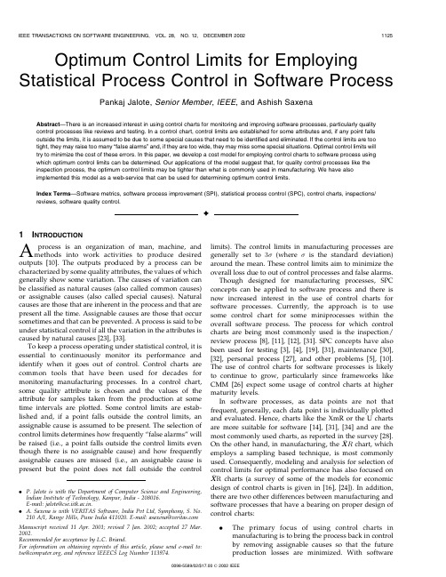
Optimum Control Limits for Employing Statistical Process Control in Software Process Pankaj Jalote,Senior Member,IEEE,and Ashish SaxenaAbstract—There is an increased interest in using control charts for monitoring and improving software processes,particularly quality control processes like reviews and testing.In a control chart,control limits are established for some attributes and,if any point falls outside the limits,it is assumed to be due to some special causes that need to be identified and eliminated.If the control limits are too tight,they may raise too many“false alarms”and,if they are too wide,they may miss some special situations.Optimal control limits will try to minimize the cost of these errors.In this paper,we develop a cost model for employing control charts to software process using which optimum control limits can be determined.Our applications of the model suggest that,for quality control processes like theinspection process,the optimum control limits may be tighter than what is commonly used in manufacturing.We have alsoimplemented this model as a web-service that can be used for determining optimum control limits.Index Terms—Software metrics,software process improvement(SPI),statistical process control(SPC),control charts,inspections/ reviews,software quality control.æ1I NTRODUCTIONA process is an organization of man,machine,andmethods into work activities to produce desired outputs[10].The outputs produced by a process can be characterized by some quality attributes,the values of which generally show some variation.The causes of variation can be classified as natural causes(also called common causes) or assignable causes(also called special causes).Natural causes are those that are inherent in the process and that are present all the time.Assignable causes are those that occur sometimes and that can be prevented.A process is said to be under statistical control if all the variation in the attributes is caused by natural causes[23],[33].To keep a process operating under statistical control,it is essential to continuously monitor its performance and identify when it goes out of control.Control charts are common tools that have been used for decades for monitoring manufacturing processes.In a control chart, some quality attribute is chosen and the values of the attribute for samples taken from the production at some time intervals are plotted.Some control limits are estab-lished and,if a point falls outside the control limits,an assignable cause is assumed to be present.The selection of control limits determines how frequently“false alarms”will be raised(i.e.,a point falls outside the control limits even though there is no assignable cause)and how frequently assignable causes are missed(i.e.,an assignable cause is present but the point does not fall outside the control limits).The control limits in manufacturing processes aregenerally set to3 (where is the standard deviation)around the mean.These control limits aim to minimize theoverall loss due to out of control processes and false alarms.Though designed for manufacturing processes,SPCconcepts can be applied to software process and there isnow increased interest in the use of control charts forsoftware processes.Currently,the approach is to usesome control chart for some miniprocesses within theoverall software process.The process for which controlcharts are being most commonly used is the inspection/review process[8],[11],[12],[31].SPC concepts have alsobeen used for testing[3],[4],[19],[31],maintenance[30],[32],personal process[27],and other problems[5],[10].The use of control charts for software processes is likelyto continue to grow,particularly since frameworks likeCMM[26]expect some usage of control charts at highermaturity levels.In software processes,as data points are not thatfrequent,generally,each data point is individually plottedand evaluated.Hence,charts like the XmR or the U chartsare more suitable for software[14],[31],[34]and are themost commonly used charts,as reported in the survey[28].On the other hand,in manufacturing,the"X R chart,whichemploys a sampling based technique,is most commonlyused.Consequently,modeling and analysis for selection ofcontrol limits for optimal performance has also focused on "X R charts(a survey of some of the models for economic design of control charts is given in[16],[24]).In addition,there are two other differences between manufacturing andsoftware processes that have a bearing on proper design ofcontrol charts:.The primary focus of using control charts in manufacturing is to bring the process back in controlby removing assignable causes so that the futureproduction losses are minimized.With software.P.Jalote is with the Department of Computer Science and Engineering, Indian Institute of Technology,Kanpur,India-208016.E-mail:jalote@cse.iitk.ac.in.. A.Saxena is with VERITAS Software,India Pvt Ltd,Symphony,S.No.210A/1,Range Hills,Pune India411020.E-mail:asaxena@Manuscript received11Apr.2001;revised7Jan.2002;accepted27Mar.2002.Recommended for acceptance by L.C.Briand.For information on obtaining reprints of this article,please send e-mail to:tse@,and reference IEEECS Log Number113974.0098-5589/02/$17.00ß2002IEEEprocesses,besides improving the process,an im-portant objective of using control charts is to controlthe product also.For example,when using controlcharts for an inspection process,if a point fallsoutside the control limits,besides the processimprovement actions like improving the checklist,inevitably,product improvement actions like rere-views,scheduling extra testing is also taken.In[14](which is perhaps the first paper on the use of SPC insoftware),Gardiner and Montgomery suggest“re-work”as one of the three actions that managementshould take if a point falls outside the control limitsThe use described in[8]clearly shows this aspect ofproduct control.The survey of high maturityorganizations also indicates that project managersalso use control charts for project-level control[21].Due to this use for product-control,project managersare more likely to want potential warning signals tobe pointed out,rather than miss such signals,even ifit means more false alarms..The cost parameters that affect the selection of control limits are likely to be quite different insoftware processes.For example,if a manufacturingprocess has to be stopped(perhaps because a pointfalls outside the control limits),the cost of doing socan be quite high.In software,on the other hand,thecost of stopping a process is minimal as elaborate“shutdown”and“startup”activities are not needed.Similarly,the cost of evaluating a point that fallsoutside the control limits is likely to be very differentin software processes as compared to manufacturingprocesses.Due to these differences,it is reasonable to assume that, to get the best results,control charts will need to be adapted to take into account the characteristics of the software process.In this paper,we examine the issue of setting control limits when control charts are used in software processes.We will focus our attention on the quality control processes,in particular,the review/inspection process. (The reader is referred to[13],[15]for further information on the inspection process.)We develop a model for applying control charts to the review ing this model,the total cost of process control as a function of control limits is determined.This cost function is then used to numerically compute the optimum control limits at which the total cost is minimized. We are now making the software available as a web service that a process designer can use to determine the optimum control limits by giving the values of the different parameters.By using the model,a process designer can set the control limits such that the overall cost of employing control charts is minimized.In the next section,we provide an overview of control charts and their use in software process,including an example.In Section3,we describe our model and the assumptions we make.The overall cost of using a control chart and determining the control limits that will minimize this cost is discussed in Section4.The section also describes how the model is numerically solved and gives the URL of an experimental software that can be used by process designers to apply this model to their process parameters. Section5gives a few examples to illustrate the use of the model.One example uses the data from a real organization and discusses how that data was collected.Sensitivity analysis of the model is discussed in Section6and Section7 contains the conclusion.2S TATISTICAL P ROCESS C ONTROLThe basis of statistical process control(SPC)is that,if a process is used consistently,it will demonstrate consistent results in key process attributes like quality,productivity, etc.[5].Consistency does not mean that the same results will always be achieved—the results will vary as there are some normal variations in the performance that are inherent to all processes.The variation that is inherent in the process is called noise or common cause variation.It is not possible to control the variation due to common causes in a process—to reduce the variation further,the process itself has to be changed.However,there are situations in which special factors are at play when the process is executing.That is,besides the common or inherent causes,there are special causes.These special causes,when present,generally cause a large variation in process performance.This change in perfor-mance due to special causes can be thought of as the signal through which these special causes can be identified and later removed.If the variation in performance of a process is only due to common causes,then it is said that the process is under statistical control,or that it is a stable process.The bounds on the performance of such a process can be predicted.On the other hand,if the process is not stable,its performance cannot be predicted as the variation due to special causes is unpredictable.The key problem of SPC is how to identify the special causes whenever they are present.This means that,from the behavior of the process,the noise has to be separated from the signal whenever there is a signal.Control charts are a means to achieve this goal.There are various types of control charts.In manufactur-ing,the most common type of control chart is the"X R chart [23],[33].For this chart,at regular time intervals,a sample consisting of a few outputs of the process is taken.For a sample,the mean("X)is the mean of the value of the attribute of interest for the outputs in this sample.The range R is the difference between the maximum and the minimum value of the attribute for the outputs in the sample.The mean values for the samples collected at different times are plotted on one chart,giving rise to the ("X)chart.The range for the samples is plotted as the R-chart.These charts are used to identify the presence of any special causes.The control limits are generally set at3 around the mean(where is the standard deviation).That is,the upper control limit(UCL)is the mean value of"X from the samples plus3 ,while the lower control limit(LCL)is mean value of "X minus3 .With these control limits,the chances that apoint will fall outside the control limits,even when there is no special cause,is only0.27percent[23],[33].Hence, whenever a point falls outside the control limits,it is highlylikely that some assignable cause is present in the process.Therefore,a point falling outside the control limits is taken to signify the presence of of an assignable cause.(Actually,there are other rules also for identifying the presence of an assignable cause [10],[23],[33].)Note that control charts are only used to identify the presence (with high probability)of special causes.They are silent on what should be done in such a situation.In the "XR chart,the mean of the values in a sample is plotted.In software,as outputs are fewer,it is usually desirable to consider and plot the attribute value for each ouptut separately.To achieve this,the XmR chart and the U-chart are well-suited [23],[33].In the XmR chart,the value of the attribute is plotted individually to form the X-chart.For range,the moving range of two consecutive points is plotted.In the U-chart,the individual data point is plotted,but there is no general control limit—a different control limit is established for each point,depending on the size of the work product (or the “area of opportunity”).However,for a process like the inspection process,approximate U-charts can be built with a single control limit by working with the average size of code that is inspected at a time [8].Let us illustrate the use of control charts for the inspection process through an example.We will focus on the X-chart.The attributes generally plotted for inspections are the preparation or inspection rate (LOC/hour)or density of defects detected during the inspection (defects/LOC).Suppose we plot defect density.Then,after each inspection,the defect density will be plotted,giving rise to a run chart.From data from previous inspections (either from the same project or from across the organizations),control limits are established.Suppose the control chart is as shown in Fig.1(adapted from [8]).As we can see,the defect density for inspection 20is more than the upper control limit.For this inspection,other parameters,like coverage rate,preparation rate,previous history of the module being reviewed,etc.,are considered.It may be found (as in [12])that the assignable cause is that new coding standards were introduced and that is why the number of defects is too high.The action following this identification could be to train the programmers in the new coding standards,as was done in [12].On the other hand,the examination might reveal that all parameters for the process are as expected and the reason the point fell outside the control limits is that the module being inspected is defect prone (as in [8]).In that case,to further control the quality of this module,action might be taken to redesign or rework the module,reinspect it,or schedule more testing [8].In general,in software processes,if a point falls outside the control limits,actions might be taken to improve the work product and/or to change the process to remove the special cause.3S YSTEM M ODELANDA SSUMPTIONSFor control charts to be effective,control limits have to be chosen carefully so they separate the normal variation from the variation caused by an assignable cause.The distribution of variation due to natural causes (often assumed to be normally distributed)is,generally,such that there is a nonzero probability for the attribute to have any value.Hence,it is not possible to set control limits that will perfectly and reliably separate the two cases.Regard-less of what control limits are set,two types of errors are possible [23],[33]:JALOTE ANDSAXENA:OPTIMUM CONTROL LIMITS FOR EMPLOYING STATISTICAL PROCESS CONTROL IN SOFTWARE PROCESS 1127Fig.1.A control chart for defect rates in inspection.1.Type1error:This error occurs when a point fallsoutside the control limits because of variation due tonatural causes themselves.This forces us to searchfor assignable cause(when none exists)and addsextra cost to the process.2.Type2error:This error occurs when a point fallsinside the control limits,although some assignablecause is present in the process.In this case,weignore this point rather than taking correctiveactions and this leads to extra cost in downstreamprocesses.It is not possible to reduce the probability of these two errors to zero.In fact,there is a tradeoff—if one increases, the other decreases.Hence,setting the control limits is a balancing act.Generally,economic factors regarding the costs of these two types of errors are considered to select the control limits.For formulating the economic model of a quality control process,we make some assumptions about the process behavior.We assume that the process starts from an incontrol state,i.e.,initially,all the variations in the process performance are due to natural causes.We assume that the main attribute being monitored is observed defect density (ODD),which is the number of defects detected per unit size(assume that size is measured in KLOC).For defect density,U-charts are more suitable as they can easily accommodate the different sizes of document/code being reviewed.However,as suggested in[10],as control limits often do not vary much for different data points,XmR charts are a reasonable and simpler alternative.Here,we consider the X-chart of ODD.We assume that ODD is distributed normally with mean 0defects per KLOC and standard deviation .That is,the average number of defects detected by this process is 0per KLOC and the actual defect density of a review is normally distributed with the mean 0and standard deviation .The process is considered as a series of control cycles. Each cycle begins with the quality process in an in-control state.After operating for some time in the in-control state, an assignable cause occurs and the process goes out of control.We assume that,when out of control,the mean of ODD shifts byÆ ,but the variance remains the same.For some time,the presence of this assignable cause goes undetected as the data points continue to fall within the control limits.Eventually,a point falls outside the control limits,generating a signal.On this signal,analysis is done to identify the cause and actions are taken to“repair”the process.Following a repair,the process returns to the in-control state and a new cycle begins.This behavior of the process is shown in Fig.2.We can also view this whole process as a failure-repair process[29].The process starts with an in-control state.In this state,if a data point falls outside the limits,some analysis is done,but the process continues to remain in the in-control state.At some point,some assignable cause occurs and the process goes in out-of-control state.It continues in this state until a data point falls outside the control limits that have been set for the process.On this signal,some analysis is done.As the process has some assignable cause,we assume that the analysis will reveal the presence of the assignable cause and the process will be repaired by removing the assignable cause.Once the assignable cause is removed,the process goes back to the in-control state.A state diagram of a control cycle is shown in Fig.3.One control cycle is:Starting from the initial in-control state,it remains in this state for some time,goes to the out-of-control state,and remains in it until a point falls outside the control limits,then returns back to an in-control state after process and product repair.A control cycle is thus an interval between two successive repairs.An optimization over a single control cycle will causes the optimization of the whole quality process since the process is a repetition of these control cycles.A cycle in the process life consists of three different stages.These stages are:process operating in an in-control state(before arrival of assignable cause),process operating1128IEEE TRANSACTIONS ON SOFTWARE ENGINEERING,VOL.28,NO.12,DECEMBER2002Fig.2.A control cycle of qualityprocess.in an out-of-control state(between the arrival and detection of assignable cause),and searching and repairing of the assignable cause.All three stages add some cost to the control cycle.(We do not model examining a false alarm as a separate state as the cost of false alarms is taken as part of the in-control state.)The cost in the in-control stage is due to a Type1error that may occur and the cost in an out-of-control stage is due to Type2errors.In the third stage,the cost is due to process repair.We assume that the average cost of analyzing a false alarm is T and the average cost of correcting an out-of-control situation is W.We assume that the process stays in an in-control state for an average of reviews.That is,on average,an assignable cause occurs after every controlled reviews.To compute the cost implications of not detecting an out-of-control situation,we need to understand what the cost is of removing a defect in the current stage versus what it will cost to remove it in later stages.We assume that the mean cost of removing a defect in this stage is C1and the mean cost of removing it later is C2.To compute the total cost,we assume that the average size of the work product is KLOC. To summarize,we use the following parameters:1.Control limit parameter k(the actual control limitsare 0Æk ).2.When the process is operating normally,the averageODD is 0and its standard deviation is .3.Amount of shift, ,in ODD due to occurrence of anassignable cause(the shift is ).4.Average number of reviews done in an in-controlstate, ,before the process goes out of control.5.Average cost of analyzing false alarm,T.6.Average cost of correcting an out of controlsituation,W.7.Average cost of fixing a defect in this phase,C1.8.Average cost of fixing a defect in later stages,C2.9.Average size of a work product being reviewed, .4S ETTING C ONTROL L IMITSThe total cost of a cycle is sum of cost of all three stages.The contribution of these costs to total cost depends on the probability of their occurrences of corresponding errors which in-turn depend on control limits.The probability of a Type2error increases with control limit and probability of a Type1error decrease and vice versa.The sum of these costs forms a U-shaped curve,which has a minimum at some value of control limits.This cost minimizing value of control limits economically balances the two costs and minimizes the total cost.Cost minimization is perhaps the most important criteria while setting the control limits.Several methods for the design of economically optimal control charts for manu-facturing processes have been suggested in the quality control literature.A detailed study of these models,most of which focus on"X R charts,is given in[7],[9],[25].Here,we present a simple cost model which is used to determine the optimal control limits in software processes.4.1False Alarm CostWhen the process operates in an in-control state,with each observed data point,there is an associated probability that it may fall outside the control limits.The points which fall outside the control limits,even when the process is actually in an in-control state,are called false alarms or false positives. On occurrence of a false alarm,the process is examined to check whether the process is in the under-control state or not.This extra examination is the False Alarm Cost(FAC).If the control limits are set atÆk distance from the mean 0,the probability that ODD of a quality process exceeds the control limits,even though the process in control is essentially the area in the probability density function from1to LCL plus the area from UCL to1.(A parameter-like defect density does not have negative values,leading to a truncated distribution.We assume that errors due to this truncation on the probabilities are negligible.)As the function is symmetric,this probability, is given by the following equation:¼2ÈðÀkÞ;ð1ÞwhereÈis the cumulative distribution function of a standard normal variable and is given byÈðzÞ¼Z zÀ1expÀx2=2ffiffiffiffiffiffi2p dx:ð2ÞPictorially, can be represented as area under parts of the normal distribution curve,as shown in Fig.4.It can be shown that,if control limits are set to3 ,then is0.0027;if the limits are2 ,then is0.0455;and,if the limits are1 , then is0.3173.As the process remains in an in-control state for an average of reviews,and the expected cost of handling a false alarm is T person hours,the expected number of reviews done in the in-control state is T .Hence,the FAC in one control cycle isFAC¼ ÂT person hours:ð3ÞNote that,for computing FAC,we do not need to consider the full length of a cycle,but only that part of the cycle during which the process is operating normally.After the shift takes place,the cost incurred till it is detected is considered next.Here,we considered that the average duration of the process staying in control is reviews.From a modeling perspective,it is perhaps better to consider “going out of control”as a Poisson process with rate. However,we have found,in our experiments,that,by doing this,the final results do not change significantly. Hence,we work only with the average.JALOTE ANDSAXENA:OPTIMUM CONTROL LIMITS FOR EMPLOYING STATISTICAL PROCESS CONTROL IN SOFTWARE PROCESS11294.2Undetected Failure CostThe reviews done between the occurrence and detection of an assignable cause are the ones in which the process is not operating normally.Due to the process being out of control, these reviews may fail to detect the expected number of defects from the work product.These defects get trans-ferred to later phases of development where the cost of removal is higher.In general,the later defects are detected, the higher the cost of fixing them.If the average cost of fixing a defect in current development phase is C1person hours and the expected cost of fixing a defect after the current phase is C2person hours,then the additional cost per such review due to this error isM¼  ÂðC2ÀC1Þ person hours;ð4Þwhere  is the shift in ODD when the process is out of control and is the average size of work product being reviewed in KLOC(   is the expected number of defects that pass through this stage).To get the total cost in a cycle,we need to determine the expected number of reviews conducted while the process is in an undetected out-of-control state.Let P be the probability that,when an assignable cause is present,the ODD will fall outside the control limits.P represents the ability of the control chart to detect an assignable cause and isð1ÀProbability of Type II errorÞ.The probability of a type II error represents the area in the shifted curve that falls within the control limits,as shown in Fig. 5. Mathematically,P¼ÈðÀ ÀkÞþÈð ÀkÞ:ð5ÞIf the shift is known,then P can be computed for a control limit.For example,if the shift is1 ,then P is0.022 with control limits set to3 ,0.16with control limits set to 2 ,and0.52with control limits set to1 .Similarly,if the shift is2 ,then P is0.158with control limits set to3 ,0.50 with control limits set to2 ,and0.842with control limits set to1 .The expected number of reviews that take place with the shifted process(i.e.,after the shift occurs but before it is detected)is1=P.Therefore,the expected undetected failure cost(UFC)for a cycle isUF C¼M=P person hours:ð6Þ4.3Repair CostWhen an assignable cause is found,certain actions are taken to remove the assignable cause and bring the process back into control.We assume that this cost is fixed at W person hour.As there is only one repair in each cycle,the total repair cost(RC)is W.4.4Optimal Control LimitsTotal cost(T C)of a control cycle is the sum of the false alarm cost,undetected failure cost,and repair cost,Total Cost;T C¼FACþUFCþRC¼ T þM=PþW¼2T ÈðÀkÞþMÈðÀ ÀkÞþÈð ÀkÞþW person hours:ð7ÞIt is clear that the total cost depends on many parameters and,if the value of the parameters are known,we can find the cost of a cycle for a given control limits.The dependence of the total cost on various parameters is shown in Fig.6.With the function for total cost known,we now address the question of minimizing the cost.It should be clear that the control limit parameter,k,is the one that influences the cost the most.Furthermore,when using a process,k is a parameter that is fully under the control of engineers and they decide what it should be,unlike most of the other parameters that are the properties of the process.For an engineer or a process designer,then,the main question is what value of k should be selected.Given the cost function, the obvious answer is to select k that will minimize the total cost.The value of k that achieves this is the optimal control limit k opt.It is hard to analytically differentiate the cost with respect to k and then determine the value of k opt.We therefore do it numerically.We have written a program that,given the value of parameters,computes the cost for different values of k and plots it.Besides the plot,it also gives the value of k opt.In one version of this implementation(available as a service at www.cse.iitk.ac.in/research/software),to simpli-fy the use of the model,for each k,we compute the cost for different values of shift(between0.5and3.0times the standard deviation)and then take the final cost as the average cost.This cost is then used to determine the optimum.5E XAMPLESLet us now illustrate determining the optimal control limits through some examples.First,let us take the data given in [10]for a code review process.The average size of code during review is0.32KLOC and the review process detects on average20.2defects/KLOC with standard deviation7.2. We assume that the process shifts on an average after every 40reviews.That is,the code review process remains stable for on an average40reviews before some assignable cause occurs.We assume that the cost of investigating a false alarm is10person hours and for finding and repairing a process is an additional10person hours.This assumption says that,if the performance of a code review falls outside the control limits,even when the review process is operating normally,it takes10person hours to examine all the data for that review and declare that there is no assignable cause. And,if the analysis shows that there is an assignable cause, the activities that need to be undertaken to modify the review process are an additional10person-hours.We1130IEEE TRANSACTIONS ON SOFTWARE ENGINEERING,VOL.28,NO.12,DECEMBER2002。
Khovanov homology torsion and thickness
1
Basic properties of Khovanov homology
The first spectacular application of the Jones polynomial (via Kauffman bracket relation) was the solution of Tait conjectures on alternating diagrams and their generalizationsm to adequate diagrams. Our method of analysing torsion in Khovanov homology has its root in work related to solutions of Tait conjectures [Ka, Mu, Thi]. Recall that the Kauffman bracket polynomial < D > of a link diagram D is defined by the skein relations < >= A < > +A−1 < > and 2 −2 <D⊔ >= (−A − A ) < D > and the normalization < >= 1. The categorification of this invariant (named by Khovanov reduced homology) is discussed in Section 7. For the (unreduced) Khovanov homology we use the
1
Partially sponsored by the NSF grant #DMS 0202613.
indicate的英语选择题

indicate的英语选择题一、单项选择题1. --- Can you please __________ the nearest supermarket on the map?--- Sure, it's marked with a red dot.A. indicateB. indicate toC. indicationD. indicating2. The traffic light turned yellow, __________ that drivers should slow down and prepare to stop.A. indicatingB. to indicateC. indicatedD. indicates3. The professor asked the students to __________ their answers with clear examples.A. indicateB. indicationC. indicating4. The signs by the poolside clearly __________ that diving is prohibited.A. indicateB. indicatedC. indicatingD. indicative5. The detective carefully observed the clues, trying to __________ the direction of the suspect's escape.A. indicateB. indicatedC. indicatingD. indication6. Anna's excellent performance in the company __________ that she is well qualified for the promotion.A. indicatesB. indicatedC. indicationD. indicating7. --- How can I __________ the correct path to the museum?--- Just follow the signs along the road.B. indicationC. indicatesD. indicate8. The arrow on the map __________ the direction to the nearest train station.A. indicatesB. indicatedC. indicationD. indicating9. The red bar on the graph __________ a significant increase in sales last month.A. indicatesB. indicatedC. indicationD. indicating10. He didn't say a word, but his facial expression clearly __________ his disappointment.A. indicatesB. indicationD. indicated二、完形填空题Humans have developed multiple ways to __11__ what they mean or convey information. One of the most common methods is through signs, symbols, and gestures. These nonverbal forms of communication serve to __12__ messages without the use of spoken language. They can __13__ a wide range of meanings depending on the context and cultural interpretations.For example, a thumbs-up gesture is often used to indicate __14__ or approval in many Western countries. On the other hand, in certain parts of the Middle East, this same gesture carries a negative connotation. __1__ it is important to be aware of cultural differences when interpreting nonverbal cues.In written communication, punctuation marks play a crucial role in indicating the __16__ of a sentence. A period at the end of a sentence indicates a complete thought, while a question mark indicates an __17__. Similarly, an exclamation point is used to indicate strong __18__. When used correctly, these punctuation marks enhance the clarity of the message being conveyed.In the field of science, color indicators are often used to __19__ the presence or absence of certain substances. For example, litmus paper turns red when it comes into contact with an acid and blue when it comes intocontact with a base. This simple color change serves as an easy __20__ to identify the nature of a substance.In conclusion, indicators, whether in the form of signs, gestures, punctuation marks, or color changes, play a crucial role in communication. They help convey messages accurately and efficiently, allowing individuals to understand and interpret information effectively. Whether consciously or unconsciously, we rely on these indicators every day to navigate our way through the world of communication.。
Parking enforcement and travel demand management

Parking enforcement and travel demand managementRomain Petiot *Groupe d’Etude et de Recherche en Economie Mathe´matique (GEREM),Universite ´de Perpignan,France Received 5July 2001;revised 3July 2003;accepted 19July 2004Available online 13October 2004AbstractThis article deals with on-street,non-free parking policy.The aim is to show how parking meter violation challenges the travel demand management policy.The literature widely admits that only the increase in the enforcement effort both deters drivers from offending and contribute to moderating car use.Nevertheless,the link between parking non-compliance,enforcement effort and travel demand has never been examined.We show that when parking meter violation behaviour,fine level choice,modal split and travel demand are connected,the fine increase paradoxically supports car use and encourages parking violation in the case of large parking congestion in particular.q 2004Elsevier Ltd.All rights reserved.Keywords:Travel policy;Modal choice;Parking policy;Parking behaviour;Parking non-compliance;Enforcement effort1.IntroductionThe literature has widely shown that parking pricing is a key feature of the urban traffic policy (Button and Verhoef,1998;Verhoef et al.,1995),especially when the aim is to moderate commuting (Higgins,1992;Shoup,1997).Yet parking meter offence is seldom dealt with.For instance,the survey by Young et al.(1991)refers neither to parking violation nor to parking enforcement.However,Cullinane and Polak (1992)show how significant the volume of parking offences is,which makes it necessary to analyse both the offender’s behaviour and the relevance of policies designed to deter parking offence.Indeed in 1990,two-thirds of the road offences in France were related to parking.The non-payment of the parking fees was particularly heavy.In Lyon,the vehicles for which the parking fee was not paid accounted for 80%of the parking offences in 1993(Lyon Parc Auto,1994).In Amsterdam,more than 50%of the commuters regularly take the risk of not paying for the parking fee and 67%of the parked hours are not paid (Mulder,1985).Despite the actual importance of parking meter violation,there are few theoretical studies on the question.However,since parking pricing is a part of the travel demand manage-ment policy,parking meter offence directly challenges the efficiency of the travel policy.Nevertheless,there are no rigorous analyses of enforcement effort to be applied within the framework of the travel policy.However,the Adiv and Wang (1987)and Elliott and Wright (1982)analyses show that—as expected—the parking non-compliance level increases as the enforcement effort decreases.This result is obtained by considering that from the driver’s point of view,illegal parking is one category of parking supply among several others.The parking choice is made as a rational economic choice (as a portfolio choice).The driver assesses the expected illegal parking cost (taking into account the enforcement proba-bility and the fine level)versus certain legal parking cost (taking into account the parking charge only).The calculus includes walking time from parking to final destination but excludes the travel demand context as traffic level or parking congestion.Then,the driver opts for the ‘cheapest’alternative between illegal and legal parking.That theore-tical result is empirically confirmed by both American (Adiv and Wang,1987)and English (Elliott and Wright,1982)data.Consequently,it seems to be an accepted fact that an increase in the enforcement effort deters parking offence.0967-070X/$-see front matter q 2004Elsevier Ltd.All rights reserved.doi:10.1016/j.tranpol.2004.07.003Transport Policy 11(2004)399–411/locate/tranpol*Address:IUT de Perpignan,De´partement GLT,Chemin de la Passio Vella,BP 79905,66962Perpignan Cedex,France.Tel.:C 33468662455;fax:C 33468662443.E-mail address:rpetiot@univ-perp.fr (R.Petiot).The aim of this article is to show that the planner should not trust that single relation between enforcement effort and non-compliance insofar as he assumes no link between the parking violation behaviour and travel demand.Actually, there are no answers concerning the impact of afine increase on travel demand.Moreover,given the relation between a parking fee increase and travel demand,it is not obvious whether afine increase is really the best answer to reduce car use when drivers do not pay for parking.Indeed, the Glazer and Niskanen(1992)and Arnott and Rowse (1999)analyses show that an increase in parking charge may yield an increase in parking turnover,which creates an additional parking supply and supports driving demand. Against all odds,parking fee increase reinforces both parking congestion and road congestion.Therefore,without a rigorous theoretical analysis concerning the impacts of the enforcement effort variation on travel demand,it is not reasonable to state that such an effect does not exist when thefine increases.We recall in Section2the aims of the parking pricing policy.Section3shows to what extent parking meter violation challenges travel policy.Section4presents some arguments against the consensus in favour of a systematic fine increase.In particular,we show that thefinancial outlook should be distinguished from an economic approach when the aim of the parking policy is to contribute to the travel demand management.Section5presents the main results of an economic analysis showing that afine increase implies a growth in road congestion and encourages non-compliance.We suggest further developments in a con-clusive point.2.The parking pricing policy2.1.The theoretical foundationsAccording to Calthrop et al.(2000),there exist two sources of inefficiency in urban transport.First,the driving cost does not reflect the actual travel cost.This market failure is dealt with by road pricing.Secondly,few individuals pay for parking.Shoup(1995)underlines that the free parking policy in the United States is generally much more implemented than parking controls.Rennes and Orfeuil(1997)assess to37%the charged on-street parking supply in Paris only.However,the Verhoef et al.(1995)analysis proves the theoretical role of parking pricing in the traffic regulation policy.When the travel cost reaches the level where the marginal social cost equals the marginal private benefit,the social travel costs are internalised and the travel demand reaches a Pareto optimal level.In particular,the total marginal social cost adds the parking social cost to the marginal social cost,which leads to reducing the optimal number of trips.Thus,the travel pricing level should apply both to road traffic and parking.Different kinds of argumentation may justify the parking pricing implemen-tation.We rank here these arguments with respect to three possible theoretical outlooks:†Parking pricing moderates road traffic but it is to be distinguished from traditional tolls.The parking price aim is not only to cover the parking social costs,but it is also to constrain demand so as to yield an optimal allocation of resources.The public road system is‘a scarce resource’and pricing is a way of giving it a price.Then,from the point of view of Bonnafous(1991)and Button(1982),parking pricing is‘a soft toll’—i.e.easier to implement and,according to Arnott et al.(1991),a more acceptable toll for commuters than road pricing.Moreover,it provides funds for investments in parking supply.†Parking pricing yields a second-best optimum on the trip market when there is no road pricing.This conclusion has been largely developed in Verhoef et al.(1995)and Button and Verhoef(1998).When traffic is not priced, drivers express demand for trips according to their private cost only without considering the marginal social cost.In economic terms,the travel market is thus inefficient.Therefore,according to Small(1992),it seems natural to conclude that free parking exacerbates this under-priced driving.Then,a parking fee equal to the marginal social cost would at least regulate parking demand.In this way,parking pricing may lead to achievea second-best on the travel market by internalisingparking externalities.Nevertheless,Glazer and Niskanen (1992)show that if parking pricing reduces the driver’s welfare by curtailing his parking time,the number of drivers being able to park increases.The new drivers’benefits may overall exceed the losses of the already parked drivers in particular when,all other thing being equal,the marginal utility of the new parking users exceeds the willingness to pay of the already parked users.Therefore,parking pricing may generate a net social welfare increase.In this way,according to the terms used by Schaefer(1994),parking pricing becomes a‘trip-end toll’.†Parking pricing may be theoretically regarded as an efficient traffic management tool as well as road pricing.In the absence of road pricing,parking pricing could internalise all the trip-related costs.Parking pricing would therefore yield afirst-best optimum.Drivers would be led to pay the actual parking cost—i.e.all the social costs related to parking including the trip costs upstream from parking.Nevertheless,Verhoef et al.(1995)show that parking pricing cannot compete with road pricing in terms of efficiency.Indeed,road pricing maximises the social welfare as it varies according to the trip characteristics—i.e.trip length,travel time,route choice,etc.These characteristics determine the marginal social cost of travel.On the other hand,parking pricing only acts upon the number of trips and modal choice,butR.Petiot/Transport Policy11(2004)399–411 400never upon route choice or trip length.Consequently,if intellectually parking pricing is potentially able to yield a social optimum,it is to be admitted that parking being located at the end of a trip,it cannot internalise the external costs upstream parking.One efficient solution is to charge all the average traffic cost externalities.However,Verhoef et al.(1995)illustrate the inefficiency of that last solution.For example,a part of the parking fees could correspond to the average external costs due to chemical emissions.Such a pricing would appear as a grant to the benefit of the longest trips which throw out the most emissions into the atmosphere to the detriment of least polluting trips.Although the two kinds of trips would decrease indeed,this tax would be socially inefficient.Finally,according to the authors,this example shows that parking pricing is efficient if the travel externality internalised is road congestion only.2.2.Parking pricing and traffic regulationAlthough parking pricing may yield a social optimum on the urban trip market,some restrictions are necessary to ensure success.Assuming that parking pricing has an impact on modal split,Gillen(1977)analyses the opportunity to substitute road pricing to parking pricing.He shows that, ceteris paribus,a parking fee variation has a rather low impact on modal choice(its elasticity measure of the driving demand with respect to the parking fee amounts to K0.31). Even though this analysis is dated,its conclusion remains interesting and it is confirmed by recent analyses(see Analytics,1995;Shaw,1997;Pratt,1999).They indicate that the elasticity of parking varies typically between K0.1 and K0.3,with significant variation depending on demo-graphic,geographic,travel choice and trip characteristics. Hensher and King(2001)also predict how an increase in parking prices in one location will shift cars to park at other locations,or travellers to shift to public transit(conclusion coming from cross-elasticity analyses).So,drivers faced with the parking fee increase may indeed switch to another trip mode or change their parking mode.Motorists substitute a relocation of their parking place for a modal shift.Only drivers already parked far from theirfinal destination switch to another transportation mode.More-over,the elasticity decreases with the distance to the city centre,simply because demand is lower there.Therefore, Gillen(1978)emphasises an overflow effect of parking pricing since,for a given distance,parking congestion is moved towards periphery.An efficient parking pricing must be continuous on a broad urban area(Gillen,1977).Thus, according to Button(1998),if parking pricing may have effects on traffic,it also has an impact on space use. For example,Arnott et al.(1991)show that the optimal parking pricing,which differs according to the parking location,partially reduces congestion.To lower their travel cost,drivers do not change their transportation mode,but try to park further indeed.The authors conclude then that the benefit in traffic management remainsfinally relatively poor.Generally speaking,the social optimum seems to be obtained by combining parking pricing and road pricing. Calthrop et al.(2000)show that this couple of policies used in a complementary way is the best way of yielding an optimum.Their theoretical simulations allow to conclude that both the parking pricing level and the road pricing level must be determined simultaneously.For van der Waerden et al.(1998),an efficient policy should be a mixture between road pricing and parking pricing.They show that this solution makes it possible to collect more than three quarters of the maximum potential welfare.This result comes from the fact that,on the one hand,parking pricing eliminates the inefficiency stemming from the parking market failures but, on the other hand,road pricing cuts down travel congestion. So,for the authors,this policy remains advantageous because road pricing does not tax the within city trips whereas parking pricing taxes the city centre trips.Nevertheless,the Glazer and Niskanen(1992)model shows that in theory,if parking pricing is likely to increase the overall drivers’surplus,this increase in parking fee cuts each driver’s parking time.Consequently,the parking time reduction generates an higher parking turnover and leads to increase parking supply.So,the increase in parking charge may contribute to increase both traffic demand and road congestion.To conclude,parking pricing is theoretically an actual tool of travel management but its economic efficiency remains relative and it should go with road pricing.Yet, parking policy is to play a part in the traffic calming policy only if it is assumed that drivers comply with the parking tariff constraints.Under the opposite assumption,what would then be the role of parking meter offences in the travel policy?Which parking enforcement effort would it be necessary to implement to reach the aims of the travel policy?3.Parking meter violation and urban mobilityGiven the role played by parking pricing in travel policy, parking meter violation interferes in the expected results of pricing policy.In economic terms,the problem lies in the interdependence between parking fee,enforcement effort, parking non-compliance and travel demand.This inter-dependence turns parking enforcement into a real tool of travel regulation policy.Therefore,both pricing and enforcement effort influence the efficiency of parking policy on the one hand,and,on the other hand,the success of traffic management.Given the relative scarcity of empirical studies consider-ing the specific impact of parking offences on mobility,one cannot say that the analysis of parking meter violation is a priority in the implementation of an effective travel policy.R.Petiot/Transport Policy11(2004)399–411401Nevertheless,a few studies provide facts and clues for further studies.In London,half of the reduction in the total travel speed downtown is due to parking offences(Elliott and Bursey, 1979).Assuming full enforcement,the reduction in the trip length in the urban area would have amounted to20%.May (1985)shows that parking non-compliance induces higher traffic and additional congestion.In addition,Rigby(1983) highlights that the road congestion induced by the parking non-compliance penalises the quality of urban transit.Indeed,parking non-compliance really seems to influ-ence mobility.However,those data are quite old.Therefore, the lack of recent works seems to prove that there exists a consensus on the link between parking non-compliance and mobility:parking violation stimulates both car use and congestion.From the viewpoint of road traffic management, the only policy to be applied is the increase in the enforcement effort,in particular thefine increase.Yet,no rigorous theoretical analyses related to the economic determinants of parking meter violation make it possible to draw such a conclusion.Therefore,it seems necessary to study the economic determinants of the parking meter violation behaviour.From such an analysis,we should be able to state on the impact of thefine increase both on non-compliance and driving demand.Afirst determinant seems to be the low degree of monitoring,control and repression.Thefigures are explicit. In Paris,out of100cars in parking offence,9arefined (Dupuy,1995).In Lyon,7.6%of the offences arefined (Lyon Parc Auto,1994)and6%of the vehicles not paying for the parking fee arefined.Thosefigures seem to be explained by the25%fall in the number of tickets per place and per month for parking offences in France between1985 and1995.The decrease seems to be explained by the20% increase in the number of places per traffic warden who enforced parking controls over the same period(Perrie`re, 1997).Therefore,it seems easy to connect the importance of parking non-compliance with an enforcement effort decrease.Then,the answer which is generally given to the question of the main determinant of parking meter violation is the weakness of the enforcement effort.As far as the travel policy is concerned,the argument is the following.If the aim is to fight against parking offence to ensure the efficiency of parking pricing,it is advisable to reinforce the enforcement effort,in particular the amount of thefine,so that the driver may think he had better pay for the parking fee.However,Adiv and Wang(1987)underline the lack of knowledge concerning the individual behaviour as regards parking meter.In particular,they underline the lack of analyses dealing specifically with the elasticity of the offending parking demand with respect to both parking fee and enforcement effort.Consequently,no one can state that the behaviour of an individual faced with an increase in the enforcement effort is systematically to comply with parking regulations.This is the reason why May(1982)claims for a better knowledge of the individuals’reactions to the enforcement effort so as to adapt repression measures which are compatible with the aims of travel management. Moreover,there are no studies stating that an increase in the enforcement effort has a positive effect on car use.The main problem is that there are no analyses dealing with the relation between parking non-compliance,enforcement effort and road congestion.4.The increase in the enforcement effort:not reallya good answerThefinancial loss derived from the offences for the parking supply manager justifiesfighting against parking non-compliance.According to a report by the French Ministry of Transportation,the average rate of payment of the parking fee is about200–900h per place over a year in French cities(DRAST,1998),while well respected,non-free parking should generate1200h paid per place per year. Half the parking supply is considered to be profitable only (Bernard and Carles,1999).According to the authors,it seems urgent to increase the enforcement effort.Yet,several remarks challenge this logic.First of all, there is no reason to think that the criterion of the parking profitability may be a sufficient argument.Admittedly,it is reasonable to advance that parking managers have a private advantage in the parking supply being profitable.Never-theless,in economic terms,achieving a higher profitability is not a relevant argument to conclude that the increase in the enforcement effort has a positive impact on the traffic calming policy.The second remark comes from a comparison which can be established between the effect of a parking fee increase and an enforcement effort increase.The theoretical results of the Glazer and Niskanen(1992)queuing model show that a parking fee increase may cause an increase in road congestion.Indeed,the authors show that a parking fee increase induces each driver to park for a shorter time.So, the increase in the parking charge contributes to a rise in the parking supply use contributingfinally to create an additional parking supply.Thereby the parking charge increase means heavier traffic.In the same way,nothing justifies claiming that an enforcement effort increase automatically results in reducing car use.Nevertheless,assuming that parking meter non-compli-ance is actually explained by the enforcement effort decrease,Perrie`re(1998)affirms that thefine level is not a sufficient incentive for the parking pricing compliance. Perrie`re(1997)notices that the on-street parkingfine in France was equivalent to10parked hours in1995while it was equivalent to20parked hours in1985.So,according to Perrie`re(1998),considering the mechanismfixing thefine level for the Parisian transit system—24times the average travel fare—the same logic should govern the calculation of thefine for parking meter violation.From11V,the parkingR.Petiot/Transport Policy11(2004)399–411 402fine should pass to30V—i.e.24times the1h parking fee in France.This statement seems really questionable as there is no reason for comparing the parking market with the Parisian transit market.For example,it does not make sense to conclude that the elasticity of offences to enforcement effort is identical on the two markets.Considering the general arguments justifying thefine increase,it should be acknowledged that nothing actually proves that such a policy is economically relevant.Without a rigorous analysis of the parking violation behaviour,it cannot be concluded that thefine increase deters parking violation and calms traffic automatically.Consequently, given the role of parking in travel demand,it is necessary to deal with the question of the offending parking enforcement with the analysis of the link between parking non-compliance and travel demand.5.The analysis of the parking meter violation behaviour: some unexpected results5.1.A parking meter violation modelIn the face the deadlock of parking enforcement with regards to the aims of travel policy,a theoretical representation of the non-compliance behaviour may lead to some sort of conclusion.The aim is to understand the individual non-compliance behaviour to improve enforce-ment effort.This analysis rests on a parking behaviour model(Arnott and Rowse,1999)presented in Appendix1.Although this model does not deal with the question of non-compliance,it formalises the link between parking conditions and travel demand.It shows how a parking pricing that internalises parking congestion changes the structure of travel demand.1 Such a formalisation is a coherent theoretical framework for integrating the question of parking meter violation.Formally,the model shows the existence of a social optimum of parking.In the case of low parking congestion, the implementation of parking pricing decentralises the social optimum by internalising parking congestion. Besides,the model shows that there is an impact of parking conditions—i.e.congestion and parking fee—on modal share and travel demand.More precisely,in the case of very high parking congestion,the equilibrium fee does not decentralise the social optimum.Arnott and Rowse(1999)then consider a parking fee variation.In this high congestion state,a parking fee increase reduces congestion in such a way that it paradoxically favours car use confirming then the results of the Glazer and Niskanen(1992)analysis.A development of the Arnott and Rowse(1999)model founded on the economics of crime(Becker,1968)integrates the parking meter non-compliance behaviour(Petiot,2000, 2002).Briefly,the driver chooses whether to pay or not to pay for the parking fee when he parks.If he does not pay,he faces the risk of a monetary sanction.If he is controlled,he pays for afine which deteriorates the welfare he gets.If he pays for the parking fee,he gets the welfare produced by his parking minus the fee.From the agent’s viewpoint,the model assumes therefore that the offending parking is a rational economic choice.A traditional cost–benefit calculation between the payment and the non-payment of the parking fee determines the agent’s choice.The agent rationally chooses the option which gets him the maximum of welfare. He compares the expected benefit he gets when he chooses not to pay with the certain benefit he gets when he chooses to pay for the parking fee.He chooses the option which curtails his expected travel cost.The purpose of the sanction is to make thefined offender bear the cost of the externality of congestion he generates when he parks but which he refuses to bear when not paying.Either the agent pays for the optimal parking fee and takes part in the internalisation of the parking externality process or he offends and does not contribute to this process if he is not controlled.When the driver is convicted guilty,he must pay for afine whose level internalises the externality of congestion he generates while parking.When paying for thefine,the agent bears all the external costs he generates while parking,proportionally to the probability of being controlled.For the purposes of analysis,we make a number of hypotheses:†Parking is assumed to be legal.The illegality involved is merely the non-payment of parking.It is interesting to see as to what extent failure to pay parking fees directly reduces the ability of parking fees to restrict car use by modifying modal split and the level of travel.In this case, thefine has the same function for the person who does not pay the parking fee as the parking fee does for the person who pays—i.e.it makes them bear the social costs their travel generates;†When apprehended a non-payer will automatically be prosecuted.The situation where the non-payer is apprehended without being prosecuted is not considered, neither is the situation where the non-payer is prosecuted only after being apprehended several times.The probability of being apprehended and the probability of being punished are therefore the same;†The duration of stay without paying the fee is the same as the length of time required to perform the activity.Non-paying parking involving a different time from that required to perform the activity is therefore not1In the Arnott and Rowse(1999)model,a commuter chooses betweentravel or not from home to destination in order to realise an activity.Hechooses to travel comparing the total travel cost(which depends on the totaltravel time)to the utility provided by the activity.If he decides to travel,hechooses to walk or drive with respect to the total travel time for each modeof transport.The total travel time by car is equal to the travel time(including the time for searching a parking place)and the parking time.Thehigher the parking congestion,the longer it takes tofind a parking place.So,the total travel time by car increases with respect to the parking congestion.R.Petiot/Transport Policy11(2004)399–411403considered,and neither is the situation where drivers park for longer than they have paid for.When the driver parks he only considers the duration of stay necessary to perform his activity.The decision to pay or not to pay the parking fee is made by considering the probability of being punished solely during this time;†The probability of punishment remains constant over the time it takes to perform the activity .It does not depend on the duration of stay to the extent that the driver parks throughout this period and only during this period.When making a decision,the driver therefore makes a calculation on the basis of the duration of stay required for the activity.The probability of being apprehended is discreet over this period and it is assumed to be known by the driver.Furthermore,the fine is a lump sum.The case of a fine that depends on the duration of stay is not considered.This conforms with reality and simplifies the calculations;†The user’s choice does not depend on the cost of enforcement .The purpose of the model is not to determine an optimum level of parking meter violations and enforcement,but,less ambitiously,to analyse the behaviour of those committing parking meter violations;†The model only considers the behaviour of a risk-neutral driver.It is obvious that analysis should consider the heterogeneity of driver behaviours with regard to risk.However,the purpose of this paper is to model the behaviour of the risk-neutral driver sufficiently accu-rately to provide a basis for future developments which will deal with different levels of risk aversion.Let A denote the ‘fee non-payment’decision.For this action,the states of nature are ‘apprehended and punished’and ‘not apprehended’.The consequences of these states of nature are,respectively,‘obtaining the satisfaction provided by parking net of the fine’and ‘obtaining the satisfaction provided by parking’.A discreet random variable Q j links the two random events,Q 1‘being apprehended and punished’and Q 2‘not being apprehended ’.It ascribes what is assumed to be a fixed probability distribution of being apprehended to the user q j,j Z 1,2such that 0%q j %1where Pj q j Z 1:Within the Arnott and Rowse (1999)model framework,if the driver does not pay the parking fee,the mean monetary benefit derived from the trip is expressed byq ðb K F ðð xA K ~x A Þ= x A ÞÞC ð1K q Þb ;where x A is the maxi-mum mean travel distance accepted by non-payers,~xA is the maximum walking distance accepted by non-payers,b is the monetary benefit derived from the trip and F is the level of the fine.The first term of the expression is the mean benefit derived from the decision not to pay the fee when the driver is punished.In this case,the satisfaction is equal to the gross gain provided by the activity at the destination minus the fine.The fine is weighed by the proportion of trips madewhich actually generate parking—i.e.ðð xA K ~x A Þ= x A Þthe modal share of driving.The mean satisfaction of thepunished non-payer is weighted by the probability q of being prosecuted.The second term expresses the benefit derived from the decision to park without paying the fee if the driver is not apprehended.This is the mean level of satisfaction of the unpunished non-payer,that is to say the gross gain generated by the trip,weighed by the probability (1K q )of not being prosecuted.The user derives no additional satisfaction from the pleasure of not paying the fee.The benefit received by the unpunished non-payer is the gross benefit derived from the trip.When the behaviour of a risk-neutral driver is repre-sented by a linear increasing utility function of the type U (x )Z x ,the non-payer maximises the trip’s hourly expected utility,which is expressed as follows:max x A ;~x A ;d A EU A Z qb K F ðð x A K ~x A = x A ÞL A C ð1K q ÞbL A;(1)where F O 0,and L A is the total travel time of non-payers.If we state that D h L A xA and X A Z b K F ðð x A K ~x A Þ= x A Þ;d A is the distance the non-paying driver cruises to find a parking space,T 1is the travel time if the trip is made by foot and T 2is the travel time if the trip is made by car (see Appendix 1),the first order conditions are as follows:v EU A v ~x A Z 1D A q F K X ALA ðT 1K T 2ÞC ð1K q ÞK bL A ðT 1K T 2Þ !Z 0;ð2a Þv EU A v x A Z 1D A q b K F K X AL AðT 2C l ÞC ð1K q Þb K bL AðT 2C l Þ !Z 0;ð2b Þv EU A v d A Z K 1D A q X A L A v T 2v d AK ð1K q Þb L A v T 2v d A !Z 0:(2c)Eq.(2a)indicates that the non-payer selects a value for ~xA which will lead to the use of a transport mode which minimises the expected cost of the trip.Eq.(2b)meansthat the non-payer selects xA so that the trip by car provides an expected benefit which covers the opportunity cost of the stly,Eq.(2c)shows that the non-payer selects the cruise distance in order to look for a parking space d A so that the value of the time spent walking to the destination does not exceed the opportunity cost of making the trip by car.We shall identify certain theoretical states of congestion for which an increase in the parking fine leads to a reduction in satisfaction which is smaller than the increase in satisfaction derived from the reduction in the parking timeR.Petiot /Transport Policy 11(2004)399–411404。
Computing crossing numbers in quadratic time
Computing Crossing Numbers in Quadratic TimeMartin GroheNovember29,2002AbstractWe show that for everyfixed there is a quadratic time algorithm that decides whether a given graph has crossing number at most and,if this is the case,computes a drawing of the graph into theplane with at most crossings.1.IntroductionHopcroft and Tarjan[13]showed in1974that planarity of graphs can be decided in linear time.It is natural to relax planarity by admitting a small number of edge-crossings in a drawing of the graph.The crossingnumber of a graph is the minimum number of edge crossings needed in a drawing of the graph into the plane.Not surprisingly,it is NP-complete to decide,given a graph and a,whether the crossing numberof is at most[12].On the other hand,for everyfixed there is a simple polynomial time algorithm deciding whether a given graph has crossing number at most:It guesses pairs of edges that cross1 and tests if the graph obtained from by adding a new vertex at each of these edge crossings is planar.The running time of this algorithm is.Downey and Fellows[7]raised the question of whether the crossing-number problem isfixed parameter-tractable,that is,whether there is a constant such that for everyfixed the problem can be solved in time.We answer this question positively with. In other words,we show that for everyfixed there is a quadratic time algorithm deciding whether a given graph has crossing number at most.Moreover,we show that if this is the case a drawing of into theplane with at most crossings can be computed in quadratic time.It is interesting to compare our result to similar results for computing the genus of a graph.(The genus of a graph is the minimum taken over the genera of all surfaces such that can be embedded into.) As for the crossing number,it is NP-complete to decide if the genus of a given graph is less than or equal to a given[18].For afixed,atfirst sight the genus problem looks much harder.It is by no means obvious how to solve it in polynomial time;this has been proved possible by Filotti,Miller,and Reif[10].In1996, Mohar[14]proved that for every there is actually a linear time algorithm deciding whether the genus of a given graph is.However,the fact that the genus problem isfixed-parameter tractable was known earlier as a direct consequence of a strong general theorem due to Robertson and Seymour[17]stating that all classes of graphs that are closed under taking minors are recognizable in cubic time.Recall that a minor of a graph is a graph obtained from a subgraph of by contracting edges.It is easy to see that the class of all graphs of genus at most is closed under taking minors.Unfortunately the class of all graphs of crossing number at most is not closed under taking minors. So in general Robertson and Seymour’s theorem cannot be applied to compute crossing numbers.An exception is the case of graphs of degree at most3;Fellows and Langston[9]observed that for such graphs Robertson and Seymour’s result immediately yields a cubic time algorithm for computing crossing numbers.2Although we cannot apply Robertson and Seymour’s result directly,the overall strategy of our algorithm is inspired by their ideas:The algorithmfirst iteratively reduces the size of the input graph until it reaches a graph of bounded tree-width,and then solves the problem on this graph.For the reductionstep,we use Robertson and Seymour’s Excluded Grid Theorem[16]together with a nice lemma due to Thomassen[19]stating that in a graph of bounded genus(and thus in a graph of bounded crossing number) every large grid contains a subgrid that,in some precise sense,lies“flat”in the graph.Such aflat grid does not essentially contribute to the crossing number and can therefore be contracted.For the remaining problem on graphs of bounded tree-width we apply a theorem due to Courcelle[4]stating that all properties of graphs that are expressible in monadic second-order logic are decidable in linear time on graphs of bounded tree-width.Let me remark that the hidden constant in the quadratic upper bound for the running time of our algo-rithm heavily depends on.As a matter of fact,the running time is,where is at least doubly exponential.Thus our algorithm is only of theoretical interest.2.PreliminariesGraphs in this paper are undirected and loop-free,but they may have multiple edges.3The vertex set of a graph is denoted by,the edge set by.We always assume that.For graphs and we let andboth endpoints of are contained in.A subgraph of a graph is a graph withand.We formally treat paths and cycles in a graph as subgraphs of this graph(as opposed to, say,sequences of vertices).Paths and cycles are always simple,that is,they have no self-intersections. 2.1.Topological Embeddings.A topological embedding of a graph into a graph is a mapping that associates a vertex with every and a path in with every in such a way that:–For distinct vertices,the vertices and are distinct.–For distinct edges,the paths and are internally disjoint(that is,they have at most their endpoints in common).–For every edge with endpoints and,the two endpoints of the path are and ,and for all.We let be the subgraph of consisting of the images of the vertices and edges of under. Formally,.2.2.Drawings and Crossing Numbers.A drawing of a graph is a mapping that associates with every vertex a point and with every edge a simple curve in in such a way that:–For distinct vertices,the points and are distinct.–For distinct edges,the curves and have at most one interior point in common (and possibly their endpoints).–For every edge with endpoints and,the two endpoints of the curve are and ,and for all.–At most two edges intersect in one point.Formally,for all .We let.An with is called a crossing of.The crossing number of is the number of crossings of.A drawing of crossing number0is called plane.The crossing number of a graph is the minimum taken over the crossing numbers of all drawings of.A graph of crossing number0is called planar.Figure 1.The hexagonal grids2.3.Hexagonal Grids.For ,we let be the hexagonal grid of radius .Instead of giving a formal definition,we refer the reader to Figure 1to see what this means.The principal cycles of are the the concentric cycles,numbered from the interior to the exterior (see Figure 2).C 1C C 32Figure 2.The principal cycles of2.4.Flat Grids in a Graph.For graphs ,an -component (of )is either a connected component of together with all edges connecting with and their endpoints in or an edge in whose endpoints are both in together with its endpoints.The vertices in the intersection of an -component with are called the vertices of attachment of the component.Let be a graph and a topological embedding.The interior of is the subgraph (remember that is the outermost principal cycle of ).A proper -component is an -component that has at least one vertex of attachment in the interior of .The topological embedding is flat if the union of with all its proper components is a planar graph.We shall use the following theorem due to Thomassen [19].Actually,Thomassen stated the result for the genus of a graph rather than its crossing number.However,it is easy to see that the crossing number of a graph is an upper bound for its genus.Theorem 1(Thomassen [19]).For allthere is an such that the following holds:If is a graph of crossing number at most anda topological embedding,then there is a subgrid such that the restriction of to is flat.2.5.Tree-Width.We assume that reader is familiar with the notion tree-width (of a graph).It is no big problem if not;we never really work with tree-width,but just take it as a black box in Theorems 2–4.Robertson and Seymour’s deep Excluded Grid Theorem [16]states that every graph of sufficiently large tree-width contains the homeomorphic image of a large grid.We use the following algorithmic version of this theorem.Theorem2.(Robertson and Seymour[17],Bodlaender[1],Perkovi´c and Reed[15]).Let.Then there is a and a linear time algorithm that,given a graph,either(correctly)recognizes that the tree-width of is at most or computes a topological embedding.Robertson and Seymour[17]gave a quadratic time algorithm,but they pointed out that it can be im-proved to linear time using Bodlaender’s[1]linear time algorithm for computing tree-decompositions. However,this improvement is not entirely straightforward:Let usfix a constant.The essential part of Robertson and Seymour’s algorithm for the problem stated in the theorem is a quadratic time algorithm that,given a graph,returns a tree-decomposition of of width at most if the tree-width of the input graph is at most.Furthermore,the algorithm returns a“counterexample”subgraph of of tree-width larger than and at most if the tree-width of is greater than.This counterexample is very important here because the subgraph is then used tofind the topological embedding of into.Bodlaender[1]gave a linear time algorithm computing a tree-decomposition of width at most if the tree-width of the input graph is at most,but his algorithm does not return a counterexample if the tree-width of is greater than.Perkovi´c and Reed[15]extended Bodlaender’s algorithm in such a way that it still works in linear time,but does return a counterexample if the tree-width of the input graph is greater than.2.6.Courcelle’s Theorem.Courcelle’s theorem states that properties of graphs definable in Monadic Second-Order Logic MSO can be checked in linear time on input graphs of bounded tree-width.In this logical context we consider graphs as relational structures of vocabulary,where and are unary relation symbols interpreted by the vertex set and edge set of a graph and is a binary relation symbol interpreted by the incidence relation.To simplify the notation,for a graph we let and call the universe of.I assume that the reader is familiar with the definition of MSO.However,for those who are not I have included it in Appendix A.Theorem3(Courcelle[4]).Let and letbe an MSO-formula.Then there is a linear time algorithm that,given a graph of tree-width at most and,,decides whether.We shall also use the following strengthening of Courcelle’s theorem,a proof of which can be found in [11]:Theorem4.Let and letbe an MSO-formula.Then there is a linear time algorithm that,given a graph of tree-width at most and,,decides if there exist,such thatand,if this is the case,computes such elements and sets.3.The AlgorithmFor an,a graph,and a subset of forbidden edges,an-good drawing of with respect to is a drawing of of crossing number at most such that no forbidden edges are involved in any crossings,that is,for every crossing of we have.Wefix a for the whole section.We shall describe an algorithm that solves the following gener-alized-crossing number problem in quadratic time:Input:Graph and subset.Problem:Decide if has a-good drawing with respect to.Later,we shall extend our algorithm in such a way that it actually computes a-good drawing if there exists one.Our algorithm works in two phases.In thefirst,it iteratively reduces the size of the input graph until it obtains a graph whose tree-width is bounded by a constant only depending on.Then,in the second phase,it solves the problem on this graph of bounded tree-width.3.1.Phase I.We let and choose sufficiently large such that for every graph of crossing number at most and every topological embedding there is a subgrid such that the restriction of to isflat.Such an exists by Theorem1.Then we choose with respect to according to Theorem2such that we have a linear time algorithm that,given a graph of tree-width greater than,finds a topological embedding.We keepfixed for the rest of the section.Lemma5.There is a linear time algorithm that,given a graph,either recognizes that the crossing number of is greater than,or recognizes that the tree-width of is at most,or computes aflat topological embedding.Proof:Wefirst apply the algorithm of Theorem2.If it recognizes that the tree-width of the input graph is at most,we are done.Otherwise,it computes a topological embedding.By our choice of ,we know that either the crossing number of is greater than or there is a subgrid such that the restriction of to isflat.For each we can decide whether isflat by a planarity test,which is possible in linear time[13].Our algorithm tests whether isflat for all.Either itfinds aflat,or the crossing number of is greater than.4Since is afixed constant,the overall running time is linear.Let be a graph and a topological embedding.For,we let be the subgrid of bounded by the th principal cycle.We let be the subgraph of consisting ofand all-components all of whose vertices of attachment are in.Moreover,we let be the subgraph of consisting of and all-components all of whose vertices of attachment are in .In particular,we call the subgraph the kernel of,the boundary of the kernel,and the interior of the kernel(see Figure3).Lemma6.Let be a graph,,and let be a-good drawing of with respect to of minimum crossing number.Let be aflat topological embedding.Then none of the edges of the kernel of is involved in any crossing of.To understand the significance of this lemma,note that theflatness of the topological embedding guarantees that the graph is planar for all.However,this does not necessarily mean that the restriction of the specific drawing to is plane.The lemma implies that at least the restriction of to the kernel is plane(the actual statement of the lemma is slightly stronger).Proof:For,the th ring of is the subgraph of consisting of and(the images of the th and th principal cycle)and the images of all edges in connecting these two cycles(see Figure4).Then for with,the graphs and are disjoint. Recall that.Since at most two edges are involved in any crossing,by the pigeonhole-principle there is an such that none of the edges in is involved in any crossing of. Let,,,and.Then and are both connected planar graphs.Let be the-component that contains.Thus consists of,all edges connecting to,and the endpoints of these edges.(Recall the definition of an-component of a graph from the beginning of Subsection2.4.)Note that the vertices of attachment of are all on.Figure3.Aflat grid in a graph,its kernel,and the boundary of the kernelFigure4.The ring in a gridWithout loss of generality we can assume that is connected.Then the graph consists of the boundary and one connected component EXT that contains the exterior part of the grid(in particular the cycle—recall that)and the rest of.consists of the cycle and possibly additional -components.Let usfirst consider the restriction of to.Claim1:There exists a connected component of such that the-images of all vertices of attachment of are on the boundary of.Proof:Since is a cycle and none of the edges of is involved in any crossing of,is a simple closed curve in the plane.Furthermore,since EXT is a connected graph,EXT must be entirely contained in one connected component of,say,in the exterior.Let be the interior of.Then must be contained in(except for its vertices of attachment,which are on the boundary of).To see this,suppose for contradiction that is not contained in.Since is a connected graph and none of the edges of the ring is involved in any crossing of,either is contained in the-image one of the hexagons of the ring,or it is contained in the exterior of the ring.But this can both not happen,because the vertices of attachment of are on,and they are not contained in the boundary of a single hexagon.So is contained in.Now if(that is,if there are no components),or if maps all components to the exterior of,then is a connected component of such that the-images of all vertices of attachment of are on the boundary of.But in general,may map some of the components to .Suppose for contradiction that there are two connected component of such that the boundary of both contains the image of a vertex of attachment of.Since is connected,there is a path connecting these two vertices,and must intersect.This contradicts the fact that noneof the edges of is involved in any crossing of.Claim2:The restriction of to is plane.Proof:Suppose for contradiction that this is not the case.Then two edges of must cross under.Let be a plane drawing of the planar graph.Let be the the connected component ofthat contains.Without loss of generality we can assume that is not the exterior component,that is, is homeomorphic to an open disc.Similarly we can assume that the set of Claim1is homeomorphic to an open disc.Let be the vertices of attachment of,and let be a homeomorphism fromto.We define a new drawing of by letting on and on.Then no edges of are involved in any crossing of,thus the crossing number of is smaller than that of.This contradicts the minimality of the crossing number of and proves Claim2.Claim3:None of the edges of is involved in any crossing of.Proof:Since the restriction of to is plane,and since none of the edges of is involved in any crossing,the only possible crossing involving an edge of would be between an edge of EXT and an edge of.But since and EXT are embedded into different components of(we showed this in the proof of Claim1),each such crossing would induce a crossing with an edge of.So there cannot be any such crossings,and Claim3is proved.To complete the proof of the lemma,we just recall that the kernel is a subgraph of.Now we are ready to describe the main reduction step our algorithm performs.Lemma7.There is a linear time algorithm that,given a graph and an edge set,either recognizes that the crossing number of is greater than,or recognizes that the tree-width of is at most,or computes a graph and an edge set such that,and has a-good drawing with respect to if,and only if,has a-good drawing with respect to.Proof:Wefirst apply the algorithm of Lemma5.If it tells us that the crossing number of is greater than or that the tree-width of is at most,there is nothing else we need to do.So suppose the algorithm returns aflat topological embedding.Let be the kernel of,its interior,and its boundary.Let the graph obtained from by contracting the connected subgraph to a single vertex(see Figure5).5Figure5.The transformation from a graph toLet be the union of with the set of all edges of and all edges incident with the new vertex.I claim that has a-good drawing with respect to if,and only if,has a-good drawing with respect to.The forward direction of this claim follows from Lemma6.For the backward direction we observethat every-good drawing of with respect to can be turned into a-good drawing of with respect to by embedding the planar graph into a small neighborhood of.Clearly,given and,the graph and the edge-set can be computed in linear time.Moreover .This yields the desired algorithmIterating the algorithm of the lemma,we obtain:Corollary8.There is a quadratic time algorithm that,given a graph,either recognizes that the crossing number of is greater than or computes a graph and an edge set such that the tree-width of is at most and has a-good drawing with respect to if,and only if,has a-good drawing with respect to.3.2.Phase II.If the algorithm has not found out that the graph has crossing number greater than in Phase I,it has produced a graph of tree-width at most and a set such that has a-good drawing with respect to if,and only if,has a-good drawing with respect to.In Phase II,the algorithm has to decide whether has a-good drawing with respect ing Courcelle’s Theorem3,we prove that this can be done in linear time.To this end,we shallfind an MSO-formula such that for every graph and every setwe have if,and only if,has a-good drawing with respect to.We rely on the well-known fact that there is an MSO-formula planar saying that a graph is planar.(Actually,this is quite easy to see:just says that neither contains nor as a topological subgraph.Also see[6].)planarFor a graph and edges that do not have an endpoint in common we let be the graph obtained from by deleting the edges and and adding a new vertex and four edges connecting with the endpoints of the edges of and in(see Figure6).Observe that for everyFigure6.A graph with selected edges and the resultinga graph has an-good drawing with respect to an edge set if,and only if,either has an-good drawing with respect to or there are edges that do not have an endpoint in common such that has an-good drawing with respect to.Lemma9.For every MSO-formula there exists an MSO-formula such that for all graphs,edge sets and edges that do not have an endpoint in common we have:This lemma can easily be proved by a standard technique from logic,the method of syntactic interpre-tations.6For readers not familiar with syntactic interpretations,a direct proof of the lemma can be found in Appendix B.Using this lemma,we inductively define,for every,formulas and such that for every graph and edge set we havehas an-good drawingwith respect toand for all,,and edges that do not have an endpoint in common we havehas an-gooddrawing with respect toWe letplanarand,for,This completes our proof that there is a quadratic time algorithm deciding if a graph has a good drawing with respect to a set.puting a Good Drawing.So far we have only proved that there is a quadratic time algorithm deciding if a graph has a good drawing.It is not hard to modify this algorithm so that it actually computes a drawing:For Phase I,we observe that if we have a good drawing of with respect to then we can easily construct a good drawing of with respect to.So we only have to worry about Phase II.By induction on,for every we define a linear-time procedure DRAW that,given a graph of tree-width at most and a subset,computes an-good drawing of with respect to(if there exists one).DRAW just has to compute a plane drawing of.For,we apply Theorem4to the MSO-formulaIt yields a linear time algorithm that,given a graph and an,computes two edgessuch that(if such edges exist).It follows immediately from the definition of that if,and only if,are in that do not have an endpoint in common andhas an-good drawing with respect to.Given and,the procedure DRAW applies this linear-time algorithm to compute edges such thatThen it applies DRAW to the graph to compute an-good drawing of a graphwith respect to.It modifies this drawing in a straightforward way to obtain an-good drawing of with respect to.Remark10.In the conference version of this paper I claimed that the use of Courcelle’s theorem in our proof can be avoided in favor of a direct algorithm that employs“the usual dynamic programming tech-niques”.Although this is true—after all,Courcelle’s algorithm also employs these dynamic programming techniques,so we can simply take the formula constructed above and extract an algorithm from Courcelle’s proof—it is not as simple as I thought then.The formula we construct essentially says:“There exists edges such that if we cross with (for)the graph does not contain a-minor or a-minor.”This statement involves a non-trivial quantifier alternation,which is what makes the translation to an algorithm difficult.At this point,I think that the route through logic and Courcelle’s theorem is essential for our proof.3.4.Uniformity.Inspection of our proofs and the proofs of the results we use shows that actually there is one algorithm that,given a graph with vertices and a non-negative integer,decides whether the crossing number of is at most in time for a suitable function.Unfortunately,grows extremely fast,at least doubly exponentially.To see this,note that the tree-width we derive a from the excluded grid theorem is exponential in.Testing whether a graph has tree-width requires time exponential in,that is,doubly exponential in.To give an upper bound on the growth of,we mainly have to analyse the running time of the algorithm we get out of Courcelle’s theorem.Its dependence on the formula is-fold exponential in the tree-width and the formula length,where is the number of quantifier alternations of the formula.The straightforward bound on the number of quantifier alternations of our formula saying that the crossing number is at most is3(independent of).There may be slight improvements reducing the running time by one or two exponentials,but as we saw our approach will not give us a running time whose dependence on is less than doubly exponential.4.ConclusionsWe have proved that for every there is a quadratic time algorithm deciding whether a given graph has crossing number at most.The running time of our algorithm in terms of is enormous,which makes the algorithm useless for practical purposes.This is partly due to the fact that the algorithm heavily relies on graph minor theory.However,knowing the crossing number problem to befixed-parameter tractable may help tofind better algorithms that are practically applicable for small values of.This has happened in a similar situation for the vertex cover problem.Thefirst proof[9]showing thefixed-parameter tractability of vertex cover used Robertson and Seymour’s theorem that classes of graphs closed under taking minors are recognizable in cubic time.Starting from there,much better algorithms have been developed;by now,vertex cover can be (practically)solved for a quite reasonable problem size(see[2]for a state-of-the-art algorithm).Although I do not expect there to be such a simple algorithm for deciding whether the crossing number of a graph is at most as there is for deciding whether there is a vertex cover of size at most,I conjecture that there is a more elementary algorithm for the crossing number problem whose running time is.Appendix A:Monadic Second Order LogicWefirst explain the syntax of MSO:We have an infinite supply of individual variables,denoted by et cetera,and also an infinite supply of set variables,denoted by,et cetera.Atomic MSO-formulas(over graphs)are formulas of the form,,,,and,where are individual variables and is a set variable.The class of MSO-formulas is defined by the following rules:–Atomic MSO-formulas are MSO-formulas.–If is an MSO-formula,then so is.–If and are MSO-formulas,then so are,,and.–If is an MSO-formula and is a variable(either an individual variable or a set variable),thenand are MSO-formulas.Let be a graph.Recall that.A-assignment is a mapping that associates an element of with every individual variable and a subset of with every set variable.We inductively define what it means that a graph together with a-assignment satisfies an MSO-formula(we write ):–,,,and endpoint of,–,–and,and similarly for,meaning“or”,and,meaning“implies”.–there exists ansuch thatdenotes the assignment with for all.–for all,,and similarly for meaning“for all”.It is easy to see that the relation only depends on the values of at the free variables of,that is,those variables not occurring in the scope of a quantifier or.We writeto indicate that the free individual variables of are among and the free set variables are among .Then for a graph and,we writeif for every assignment with and we have.A sentence is a formula without free variables.For example,for the sentencewe have if,and only if,is2-colorable.Appendix B:Proof of Lemma9For the reader’s convenience,we repeat the statement of the Lemma:For every MSO-formula there exists an MSO-formula such that for allgraphs,edge sets and edges that do not have an endpoint incommon we have:(1)Proof:Let be a graph,,and let be edges that do not have an endpoint in common.Let be the endpoints of and the endpoints of.We define a graph as follows:–The vertex set of is the set–The edge set of is the set–A vertex is an endpoint of an edge if。
interlocking
InterlockingFor use of the term in music,see Hocket .For use in elec-tronics and computing,see Interlock (engineering).In railway signalling ,an interlocking is anarrangement The tower and tracks at Deval interlocking,Des Plaines,Illinois ,in 1993of signal apparatus that prevents conflicting movements through an arrangement of tracks such as junctions or crossings.The signalling appliances and tracks are some-times collectively referred to as an interlocking plant .An interlocking is designed so that it is impossible to display a signal to proceed unless the route to be used is proven safe.In North America,the official railroad definition of inter-locking is:"An arrangement of signals and signal appli-ances so interconnected that their movements must succeed each other in proper sequence ".[1]1Configuration anduse A model board and lever machineA minimal interlocking consists of signals ,but usually in-cludes additional appliances such as points (US:switches)and derails ,and may include crossings at grade and mov-able bridges.Some of the fundamental principles of in-terlocking include:•Signals may not be operated to permit conflicting train movements to take place at the same time.•Switches and other appliances in the route must be properly 'set'(in position)before a signal may allow train movements to enter that route.•Once a route is set and a train is given a signal to pro-ceed over that route,all switches and other movable appliances in the route are locked in position until either•the train passes out of the portion of the route affected,or•the signal to proceed is withdrawn and suf-ficient time has passed to ensure that a train approaching that route has had opportunity to come to a stop before passing the signal.2HistoryRailway interlocking is of British origin,where numerous patents were granted.In June 1856,John Saxby receivedthe first patent for interlocking switches and signals.[2][3]In 1868,Saxby (of Saxby &Farmer )[4]was awarded a patent for what is known today in North America as “pre-liminary latch locking”.[5][6]Preliminary latch lockingbecame so successful that by 1873,13,000mechanicallocking levers were employed on the London and North Western Railway alone.[6][7]The first experiment with mechanical interlocking in the United States took place in 1875by J.M.Toucey and William Buchanan at Spuyten Duyvil Junction in New York on the New York Central and Hudson River Rail-road (NYC&HRR).[6][7][8]At the time,Toucey was Gen-eral Superintendent and Buchanan was Superintendent of Machinery on the NYC&HRR.Toucey and Buchanan formed the Toucey and Buchanan Interlocking Switch and Signal Company in Harrisburgh,Pennsylvania in 1878.The first important installations of their mecha-nism were on the switches and signals of the Manhattan Elevated Railroad Company and the New York Elevated Railroad Company in 1877-78.[6]Compared to Saxby’s 123INTERLOCKING TYPESdesign,Toucey and Buchanans’interlocking mechanism was more cumbersome and less sophisticated,so was not implemented very widely.[8]Union Switch and Sig-nal bought their company in 1882.[8]As technology advanced that served to augment the mus-cle strength of human beings the railway signaling in-dustry looked to incorporate these new technologies into interlockings to increase the speed of route setting,the number of appliances controlled from a single point and to expand the distance that those same appliances could be operated from the point of control.The challenge fac-ing the signal industry was achieving the same level of safety and reliability that was inherent to purely mechan-ical systems.An experimental hydro-pneumatic [9]inter-locking was installed at the Bound Brook,New Jersey junction of the Philadelphia and Reading Railroad and the Lehigh Valley Railroad in 1884.[6][7]By 1891,there were 18hydro-pneumatic plants,on six railroads,operat-ing a total of 482levers.[6]The installations worked,but there were serious defects in the design,and little saving of labour was achieved.The inventors of the hydro-pneumatic system moved for-ward to an electro-pneumatic system in 1891and this system,best identified with the Union Switch &Sig-nal Company ,was first installed on the Chicago and Northern Pacific Railroad at its drawbridge across the Chicago River .[7]By 1900,54electro-pneumatic inter-locking plants,controlling a total of 1,864interlocking levers,were in use on 13North American railroads and this type system would remain one of two viable com-peting systems into the future,although it did have the disadvantage of needing extra single-use equipment and requiring high maintenance.[7]Interlockings using electric motors for moving switches and signals became viable in 1894,when Siemens in Aus-tria installed the first such interlocking at Prerov (now in the Czech Republic).[10]Another interlocking of this type was installed in Berlin Westend in 1896.[11]In North America,the first installation of an interlocking plant us-ing electric switch machines was at Eau Claire,Wisconsin on the Chicago,St.Paul,Minneapolis and Omaha Rail-way in 1901,by General Railway Signal Company (now a unit of Alstom ,headquartered in Levallois-Perret ,near Paris).[7]By 1913,this type system had been installed on 83railroads in 35US States and Canadian Provinces,in 440interlocking plants using 21,370levers.[6]3Interlocking typesInterlockings can be categorized as mechanical,electrical (electro-mechanical or relay -based),orelectronic/computer-based.A view of the locking bed inside Deval Tower,Des Plaines,Illi-nois3.1Mechanical interlockingSee also:Lever frameIn mechanical interlocking plants,a locking bed is con-structed,consisting of steel bars forming a grid.The levers that operate switches ,derails ,signals or other appli-ances are connected to the bars running in one direction.The bars are constructed so that,if the function controlled by a given lever conflicts with that controlled by another lever,mechanical interference is set up in the cross lock-ing between the two bars,in turn preventing the conflict-ing lever movement from being made.In purely mechanical plants,the levers operate the field devices,such as signals,directly via a mechanical rod-ding or wire connection.The levers are about shoulder height since they must supply a mechanical advantage for the operator.Cross locking of levers was effected such that the extra leverage could not defeat the locking (pre-liminary latch lock).The first mechanical interlocking was installed in 1843at Bricklayers’Arms Junction ,England.[12]:73.2Electro-mechanical interlockingPower interlockings may also use mechanical locking to ensure the proper sequencing of levers,but the levers areconsiderably smaller as they themselves do not directly control the field devices.If the lever is free to move based on the locking bed,contacts on the levers actuate3.4Electronic interlocking 3the switches and signals which are operated electrically or electro-pneumatically .Before a control lever may be moved into a position which would release other levers,an indication must be received from the field element that it has actually moved into the position requested.The locking bed shown is for a General Railway Signal (GRS)power interlocking machine.3.3RelayinterlockingPart of a relay interlocking using miniature plug-in relaysInterlockings effected purely electrically (sometimes re-ferred to as "all-electric ")consist of complex circuitry made up of relays in an arrangement of relay logic that as-certain the state or position of each signal appliance.As appliances are operated,their change of position opens some circuits that lock out other appliances that would conflict with the new position.Similarly,other circuits are closed when the appliances they control become safe to operate.Equipment used for railroad signalling tends to be expensive because of its specialized nature and fail-safe design.Interlockings operated solely by electrical circuitry may be operated locally or remotely with the large mechani-cal levers of previous systems being replaced by buttons,switches or toggles on a panel or video interface.Such an interlocking may also be designed to operate without a human operator.These arrangements are termed au-tomatic interlockings ,and the approach of a train sets its own route automatically,provided no conflicting move-ments are in progress.GRS manufactured the first all-relay interlocking system in 1929.It was installed in Lincoln,Nebraska on the Chicago,Burlington and Quincy Railroad .[12]:18Entrance-Exit Interlocking (NX)was the original brand name of the first generation relay-based centralized traffic control (CTC)interlocking system introduced in 1936by GRS [13](represented in Europe by Metropolitan-Vickers ).The advent of all electric interlocking tech-nology allowed for more automated route setting proce-dures as opposed to having an operator line each part of the route manually.The NX system allowed anopera-Control panel for a US&S relay interlockingtor looking at the diagram of a complicated junction to simply push a button on the known entrance track and an-other button on the desired exit track,and the logic cir-cuitry handled all the necessary actions of commanding the underlying relay interlocking to set signals and throw switches in the proper sequence as required to provide valid route through the interlocking plant.The first NX installation was in 1937at Brunswick on the Cheshire Lines ,UK.The first US installation was on the New York Central Railroad (NYCRR)at Girard Junction,Ohio in 1937.[12]:18Another NYCRR installation was on the main line between Utica,New York and Rochester,New York ,and this was quickly followed up by three installations on the New York City Transit System in 1948.Other NX style systems were implemented by other rail-road signal providers.For example Union Route (UR)was the brand name of their vacuum tube -based NX overlay system supplied by Union Switch &Signal Co.(US&S),and introduced in 1951.[14]NX type systems and their costly pre-solid state control logic only tended to be installed in the busier or more complicated ter-minal areas where it could increase capacity and reduce staffing requirements.In a move that was popular in Eu-rope,the signalling for an entire area was condensed into a single large power signal box with a control panel in the operator’s area and the equivalent of a telephone ex-change in the floors below that combined the vital relay based interlocking logic and non-vital control logic in one place.Such advanced schemes would also include train describer and train tracking technologies.Away from complex terminals unit lever control systems remained popular until the 1980s when solid state interlocking and control systems began to replace the older relay plants of all types.3.4Electronic interlockingModern interlockings (those installed since the late 1980s)are generally solid state ,where the wired net-works of relays are replaced by software logic running on44DEFINED FORMS OFLOCKINGComputer-based controls for a modern electronic interlocking special-purpose control hardware.The fact that the logic is implemented by software rather than hard-wired cir-cuitry greatly facilitates the ability to make modifications when needed by reprogramming rather than rewiring. In many implementations this vital logic is stored as firmware or in ROM that cannot be easily altered to both resist unsafe modification and meet regulatory safety test-ing requirements.At this time there were also changes in the systems that controlled interlockings.Whereas before technologies such as NX and Automatic Route Setting required racks and racks of relays and other devices,solid state soft-ware based systems could handle such functions with less cost and physical footprint.Initially processor driven Unit Lever and NX panels could be set up to commandfield equipment of either electronic or relay type,however as display technology improved,these hard wired physical devices could be updated with visual display units,which allowed changes infield equipment be represented to the signaller without any hardware modifications.Solid State Interlocking(SSI)is the brand name of the first generation microprocessor-based interlocking devel-oped in the1980s by British Rail,GEC-General Signal and Westinghouse Signals Ltd in the UK.Second gen-eration processor-based interlockings are known by the term“Computer Based Interlocking”(CBI),[15]of which VPI(trademark of General Railway Signal,now Alstom), MicroLok(trademark of Union Switch&Signal,now Ansaldo STS),Westlock and Westrace(trademarks of Invensys Rail),and Smartlock(trademark of Alstom)are examples.4Defined forms of lockingElectric locking“The combination of one or more elec-tric locks or controlling circuits by means of which levers in an interlocking machine,or switches or other devices operated in connection with signalling and interlocking,are secured against operation un-der certain conditions.”[16]Section locking“Electric locking effective while a train occupies a given section of a route and adapted to prevent manipulation of levers that would endanger the train while it is within that section.”[16]Route locking“Electric locking taking effect when a train passes a signal and adapted to prevent manip-ulation of levers that would endanger the train while it is within the limits of the route entered.”[16] Sectional route locking“Route locking so arranged that a train,in clearing each section of the route, releases the locking affecting that section.”[16]Electric railway linesApproach locking“Electric locking effective while a train is approaching a signal that has been set for it to proceed and adapted to prevent manipulation of levers or devices that would endanger that train.”[16] Stick locking“Electric locking taking effect upon the setting of a signal for a train to proceed,released by a passing train,and adapted to prevent manipu-lation of levers that would endanger an approaching train.”[16]Indication locking“Electric locking adapted to prevent any manipulation of levers that would bring about an5unsafe condition in case a signal,switch,or other op-erated device fails to make a movement correspond-ing with that of the operating lever;or adapted di-rectly to prevent the operation of one device in case another device,to be operatedfirst,fails to make the required movement.”[16]Check locking or traffic locking“Electric locking that enforces cooperation between the Operators at two adjacent plants in such a manner that prevents op-posing signals governing the same track from being set to proceed at the same time.In addition,aftera signal has been cleared and accepted by a train,check locking prevents an opposing signal at the ad-jacent interlocking plant from being cleared until the train has passed through that plant.”[16]5Complete and incomplete inter-lockings(U.S.terminology)Interlockings allow trains to cross from one track to an-other using a turnout and a series of switches.Rail-road terminology defines the following types of inter-lockings as either complete or incomplete depending on the movements available.Although timetables generally do not identify an interlocking as one or the other,and rule books do not define the terms,the below is generally agreed upon by system crews and rules officials.Complete interlockings allow continuous movements from any track on one side of the interlocking to any track on the opposite side without the use of a reverse move within the limits of the interlocking.This is true even if there are differing numbers of tracks on opposing sides,or if the interlocking has multiple sides.Incomplete interlockings do not allow such movements as described above.Movements in an incomplete interlocking may be limited and may even require reverse movements to achieve the desired route.6References[1]Josserand,Peter;Forman,Harry Willard(1957).Rightsof Trains(5th ed.).New York:Simmons-Boardman Pub-lishing Corporation.p. 5.OCLC221677266.Defini-tions.[2]“Death of John Saxby”.Railway Age Gazette(Simmons-Boardman Publishing Corporation)54(20):1102.26 May1913.OCLC15110423.[3]Solomon,Brian(2003).Railroad Signaling.St Paul,Min-nesota:MBI Publishing Company.pp.23–24.ISBN 978-0-7603-1360-2.OCLC52464704.[4]Thefirst manufacturer of signal equipment,the predeces-sor of Westinghouse Brake and Signal Company Ltd,and today’s Westinghouse Rail Systems,Ltd.(headquartered in Chippenham,Wiltshire)[5]US patent80878,John Saxby&John Stinson Farmer,“Improved Switch and Signal”,issued11August1868 [6]“Landmarks in Signaling History”.Railway Age Gazette(Simmons-Boardman Publishing Corporation)61(4): 161.28July1916.[7]General Railway Signal Company(1913).Sperry,HenryM.,ed.Electric Interlocking Handbook.Rochester,New York:General Railway Signal Company.pp.5–12.OCLC3527846.[8]Calvert,J.B.“Toucey and Buchanan Interlocking”.Rail-ways:History,Signalling,Engineering.Retrieved28De-cember2011.[9]A system whereby compressed water and air are used totransmit action from one end of a long tube to the other end.It can be effective,but it still qualifies as a mechan-ical system since the pressure is pre-loaded,and requires human action of the same sort that a pure mechanical sys-tem requires.[10]Lexikon der gesamten Technik,entry“Stellwerke”[11]“Berliner Stellwerke”.Retrieved24November2012.[12]Alstom Signaling Incorporated(2004).A Centennial:History of Alstom Signaling Inc.West Henrietta,New York:Alstom.Retrieved27December2011.[13]General Railway Signal Company(1936).The NX Systemof Electric Interlocking.Rochester,New York.OCLC 184909207.[14]US patent2567887,Ronald A.McCann,“Entrance-exitroute interlocking control apparatus”,issued11Septem-ber1951,assigned to The Union Switch and Signal Com-pany[15]Woolford,Paul(April2004).Glossary of SignallingTerms(Report).Railway Group Guidance Note GK/GN0802.London:Rail Safety and Standards Board.Retrieved27December2011.[16]Defined by the Railway Signal Association,which todayis the Railway Signal Committee of the Association of American Railroads.•Elliott,W.H.(1896).Block and Interlocking Signals.New York:Locomotive Engineering.pp.143ff.•Ganguly,Sri Subhasis.“History of Railway Sig-nalling.”Accessed2011-05-06.•Solomon,Brian(2010).Railroad Signaling.Min-neapolis,MN:Voyageur Press.pp.23ff.ISBN 978-0-7603-3881-0.67EXTERNAL LINKS 7External links•Calvert,J.B.“Principles of Interlocking.”•Interlocking(1927New Zealand article by A.S.Henderson)•Kleinstadt.zip“Full free version of an interlockingplant based on German Relay Principles”(English,German,Dutch,French languages)7 8Text and image sources,contributors,and licenses8.1Text•Interlocking Source:/wiki/Interlocking?oldid=647734074Contributors:CORNELIUSSEON,Hyacinth,Cecropia, Vaoverland,Leonard G.,MisterSheik,Spearhead,Slambo,SPUI,Danhash,Ae-a,Tabletop,Lensovet,SchuminWeb,Wongm,Hairy Dude, Casey56,Gaius Cornelius,Bota47,JonRoma,Sturmovik,Attilios,SmackBot,Alfa80,Badger151,Whpq,Behemoth14,Henning Makholm, JackLumber,Peter Horn,Amakuru,CmdrObot,Thijs!bot,WillMak050389,Grahamdubya,Luna Santin,Arsenikk,MER-C,NE2,7sev-ern7,R sirahata,Keith D,Archolman,Numbo3,LordAnubisBOT,SriMesh,Signalhead,Hugo999,John Darrow,Broadbot,Truthanado, Deconstructhis,SieBot,A.Carty,Sfan00IMG,NEC Conductor,Tam0031,Addbot,Lightbot,Zeugma fr,Yobot,TaBOT-zerem,Railcon-sultant~enwiki,Steenth,Caseyjonz,AnomieBOT,Neurolysis,FrescoBot,Jonesey95,WildBot,Sk jmp,Tommy2010,Sf5xeplus,Many-marimbas,Helpful Pixie Bot,Aaron-Tripel,Marcucciboy2,Reza1552,Haraldmmueller,Carlos118and Anonymous:338.2Images•File:Ambox_globe_content.svg Source:/wikipedia/commons/b/bd/Ambox_globe_content.svg License: Public domain Contributors:Own work,using File:Information icon3.svg and File:Earth clip art.svg Original artist:penubag•File:Antwerpen_Noord_seinhuis.jpg Source:/wikipedia/commons/e/ee/Antwerpen_Noord_seinhuis.jpg License:CC BY-SA3.0Contributors:Own work Original artist:Smiley.toerist•File:Des_Plaines_interlocking_tower.jpg Source:/wikipedia/commons/e/ed/Des_Plaines_interlocking_ tower.jpg License:CC BY-SA2.5Contributors:?Original artist:?•File:Electric_railway_lines.jpg Source:/wikipedia/commons/4/4b/Electric_railway_lines.jpg License:CC BY-SA3.0Contributors:Own work Original artist:Shubham kumar singh•File:Interlocking_machine_locking_bed.jpg Source:/wikipedia/commons/d/da/Interlocking_machine_ locking_bed.jpg License:CC BY-SA2.5Contributors:Own work Original artist:JonRoma•File:Pennsylvania_Railroad,_HOLMES_Block_Station_modelboard_and_lever_machine.jpg Source:http://upload.wikimedia.org/wikipedia/en/2/2a/Pennsylvania_Railroad%2C_HOLMES_Block_Station_modelboard_and_lever_machine.jpg License:PD Con-tributors:?Original artist:?•File:Promenade_St_Tower_Control_Panel.jpg Source:/wikipedia/commons/2/2e/Promenade_St_ Tower_Control_Panel.jpg License:Public domain Contributors:Library of Congress Prints and Photograph Division,Historic American Engineering Record./pictures/item/RI0376/Original artist:William E.Barrett•File:Relay_room.jpg Source:/wikipedia/commons/b/be/Relay_room.jpg License:CC-BY-SA-3.0Contrib-utors:Transferred from en.wikipedia to Commons by Kafuffle using CommonsHelper.Original artist:Signalhead at English Wikipedia 8.3Content license•Creative Commons Attribution-Share Alike3.0。
2024年高考英语一轮复习第45讲图表类和图画类(核心考点)

第45讲图表类和图画类书面表达(核心考点精讲精练)1. 三年真题应用文考点细目表试卷年份体裁话题题材内容新高考Ⅰ/Ⅱ卷2023建议信学校生活给外教提建议全国甲卷2023投稿历史文化介绍中国历史人物全国乙卷2023投稿生活学习假期习得新技能全国卷Ⅰ/全国乙卷2022投稿调查结果学习英语的状况2021演讲稿社会科技明智的在线学习者2020记叙文身边的人值得尊敬和爱戴的人2019申请信社会实践当志愿者全国卷Ⅱ/全国甲卷2022投稿世界海洋日保护海洋2021求助信文化习俗外国朋友感兴趣的中国传统文化2020记叙文文体活动介绍采摘活动2019电子邮件文体活动排球比赛安排全国卷Ⅲ2020求助信文体活动请外教指导短剧改编2019邀请信文体活动校园音乐节2. 命题规律及备考策略【命题规律】近3年命题规律:1.内容上选材贴近考生实际生活。
所写内容都是学生熟悉内容,让学生有话可说,利于学生表达;2.体裁上有:提纲作文;开放性作文;图表作文;看图作文【备考策略】1.熟练掌握各种应用文的基本构架;2.积累基本词汇和句式,尤其是简单基本句式,写好简单句;3.背诵优美的段落和范文,模仿高级句式和表达;4.加强审题(主题、时态)训练;5.练习书写,达到整洁美观的程度。
【命题预测】预测2024年应用文考查仍然贴近考生实际生活,以电子邮件和投稿为主,考查考生的解决问题能力。
题型总览图表类图表类书面表达常用词汇1. 点明图表所反映的主题时常用的词汇:table 表格,chart 图表,diagram 图解/示意图,figure图形/数字,describe 描述,tell 告诉,show 表明,represent 描绘/展示,indicate 显示2. 分析数据差异及变化趋势时常用的词汇:(1)表示上升或增加的:rise, increase, go up(2)表示下降或减少的:decrease, fall, reduce, decline, drop, go down(3)表示变化特点的:sharply 急剧地,quickly 迅速地,rapidly 快速地,dramatically 戏剧性地,slowly 缓慢地,gradually 逐渐地。
Statistics of Self-Crossings and Avoided Crossings of Periodic Orbits in the Hadamard-Gutzw
a r X i v :n l i n /0206023v 1 [n l i n .C D ] 14 J u n 2002Statistics of Self-Crossings and Avoided Crossings of Periodic Orbits in theHadamard-Gutzwiller ModelPeter A.Braun,Stefan Heusler,Sebastian M¨u ller,and Fritz HaakeFachbereich Physik,Universit¨a t Essen,45117Essen,Germany(February 8,2008)Employing symbolic dynamics for geodesic motion on the tesselated pseudosphere,the so-calledHadamard-Gutzwiller model,we construct extremely long periodic orbits without compromisingaccuracy.We establish criteria for such long orbits to behave ergodically and to yield reliablestatistics for self-crossings and avoided crossings.Self-encounters of periodic orbits are reflected incertain patterns within symbol sequences,and these allow for analytic treatment of the crossingstatistics.In particular,the distributions of crossing angles and avoided-crossing widths thus comeout as related by analytic continuation.Moreover,the action difference for Sieber-Richter pairs oforbits (one orbit has a self-crossing which the other narrowly avoids and otherwise the orbits lookvery nearly the same)results to all orders in the crossing angle.These findings may be helpful forextending the work of Sieber and Richter towards a fuller understanding of the classical basis ofquantum spectral fluctuations.I.INTRODUCTION Billiards on surfaces of negative curvature were first investigated by J.Hadamard [1].The case of constant negative curvature,known as the pseudosphere,has enjoyed considerable popularity since Gutzwiller’s realization [2]of its potential as a paradigm of quantum plete hyperbolicity,the availability of symbolic dynamics,the equality of the Lyapunov exponents of all periodic orbits,and the validity of Selberg’s trace formula are among the attractive features of that eful introductions can be found in Refs.[3–6].For a tesselation by maximally desymmetrized octagons (see below)Aurich and Steiner found the spectral fluctuations of the quantum energy spectrum faithful to the Gaussian orthogonal ensemble (GOE)of random-matrix theory [7],as illustrated in Fig.1for the so-called form factor,the Fourier transform of the energy dependent two-point correlator of the density of levels.One of the urgent problems in quantum chaology is to understand the rather universal validity of random-matrix type spectral fluctuations for chaotic dynamical systems,nowadays known as the Bohigas-Giannoni-Schmit conjecture [8].An important first step was made by Berry [9]on the basis of Gutzwiller’s trace formula [10]which expresses the oscillatory part of the density of energy levels as a sum over periodic orbits,d osc (E )=Re γA γe i S γ/¯h ,with S γthe action and A γa classical stability amplitude of the periodic orbit γ.Berry realized that the double sum over periodic orbits in the form factor,which involves the building block A γA ∗γ′e i(S γ−S γ′)/¯h in each summand,must draw an important contribution from the diagonal terms γ=γ′since pairs of orbits with action differences larger than Planck’s unit ¯h can be expected to interfere destructively and thus to cancel in the form factor.For time reversal invariant systems each orbit γand its time reverse γTR have equal action such that Berry’s “diagonal approximation”generalizes to include pairs of mutually time reversed orbits and then gives the time dependent form factor as K (τ)=2τ+...where τis the time in units of the so called Heisenberg time,which is given in terms of the mean level density ¯d (E )as T H (E )=2π¯h ¯d(E ).Recently,Sieber and Richter [11,12]employed the pseudosphere in their pioneering move beyond the diagonal approximation;they found a one-parameter family of orbit pairs within which the action difference can be steered to zero.One orbit within each “Sieber-Richter pair”undergoes a small-angle self-crossing which the partner orbit narrowly avoids.The form factor receives the contribution K 1off(τ)=−2τ2from the family.Together with Berry’s K diag (τ)=2τwe thus have a semiclassical understanding of at least the first two terms in the Taylor series of the random-matrix form factor [13]K GOE (τ)=2τ−τln(1+2τ).The search is now on for further families of orbit pairs which might yield the higher-order terms of the expansion.At the same time,one would like and will eventually have to go beyond the pseudosphere,in order to find the conditions for universal behavior;interesting first steps have been taken for quantum graphs [14]and other billiards [15].In the present paper we remain with the pseudosphere for a thorough investigation of action correlations which we feel necessary as a basis for further progress towards an understanding of the random-matrix like spectral fluctuations in this prototypical dynamical system (and beyond).We shall make extensive use of symbolic dynamics in (i)establishing a certain local character of the relation between an orbit and its symbol sequence (only a section of the symbol sequence is necessary to determine the associated section of the orbit),(ii)constructing very long periodic orbits (up to hundreds of thousands of symbols)with full control of accuracy,(iii)identifying the ergodic ones among them and establishing a simple and instructive rederivation of Huber’s exponential-proliferation law,(iv)expressing the angle ǫof a self-crossing and the closest-approach distance δin the partner orbit of a Sieber-Richter pair in terms of the M¨o bius-transformation matrices associated with the loops joined in a crossing,(v)revealing a useful analytic-continuation kinship of ǫand δ,(vi)explicitly relating the joint density P (ǫ,l |L )for crossing angles and loop lengths l in orbits of total length L to the associated density P a (δ,l |L )for avoided crossings,and (vii)constructing an expression for the action difference of a Sieber-Richter pair valid to all orders in ǫ.Some of our findings are based on (overwhelming and exceptionless)numerical evidence based on large numbers of long periodic orbits and thus call for mathematical substantiation.Even though we strictly confine ourselves to the pseudosphere we expect (and have indeed begun to check)gener-alizability to other systems for which symbolic dynamics is available.0.0 1.02.03.04.00.01.02.0FIG.1.Form factor K (τ)for an asymmetric octagon based on energy levels determined by Aurich and Steiner [7],after averaging over a time window ∆τ=0.01.Smooth line for GOE.II.THE HADAMARD-GUTZWILLER MODELThe Hadamard-Gutzwiller model [4,7]is a two-dimensional billiard on the so called Poincar´e disc,i.e.the unit disc x 2+y 2=|z |2≤1endowed with the metric ds 2=4dx 2+dy 2(1−|z |2)2.(2.1)The distance d (z 1,z 2)between two points z 1,z 2,measured along the unique geodesic connecting them,readscosh d (z 1,z 2)=1+2|z 1−z 2|2αz+βz′=M(z):=2β∗ α−α∗±.(2.6)2The inverse M−1of a matrix M is obtained by the replacementα→α∗,β→−βin(2.3).These two matrices have their stable and unstable points interchanged.Consequently,a matrix and its inverse shift points along their common “own”geodesic by the same distance but in opposite directions.To obtain a model with compact configuration space the Poincar´e disc is tesselated with tiles of equal area and shape.Each type of tesselation is connected with a particular discrete infinite subgroupΓof SU(1,1)such that by acting on all inner points of a tile by somefixed matrix W=1we get all inner points of some other tile;the boundaries are mapped to boundaries of the same or other ing all W∈Γwe get all tiles and restore the whole disc from a single initial tile.A particular tile is distinguished by containing the origin z=0and is called the fundamental domain.In fact,different tiles are identified by identifying each point z of the Poincar´e disc with all its images W(z),and so a compact configuration space is indeed arrived at.In the present paper we exclusively work with octagonal tiles which are all identified with the fundamental domain. The opposite sides of the latter are glued together such that we arrive at a Riemann surface of genus2,i.e.a two-hole doughnut.Matrices W giving rise to octagonal tiles are arbitrary products of four elementary group elements l0,l1,l2,l3∈SU(1,1)and their inverses.For simplicity,we shall mostly consider tesselation with“regular octagons”(Fig.2)which have the highest possible symmetry;the pertinent elementary matrices l k,k=0,1,2,3,are√2 (2.7)l k= 1+√2+2√2+2and their inverses.The inverse of l k is easily checked to be l k+4.Since the index k describes a phase in the off-diagonal matrix elements we conclude=l k+4=l(k+4)mod8≡l¯k,(2.8)l−1kwhere we have introduced¯k=(k+4)mod8.The full set of elementary matrices is thus l k,k=0, (7)The sides of the boundary of the fundamental domain can now be labeled0,1,...,7and constructed as follows. Tesselation identifies opposite sides of the regular octagon as0≡4,1≡5,2≡6,and3≡7.Points on side k+4 are thus images of their mirror symmetric counterparts on side k;the group element responsible for such imaging is l k+4.In particular,the points on side0solve the quadratic equation l4(z)=−z∗and form a circle of radius 2−1/2−2−1 1/2,which is in fact a geodesic.Side k is obtained by a rotation of side0by kπ/8.>>FIG.2.Poincar´e disc and its tesselation with regular octagons.Elementary matrices other than l k+4lead from points on side k of the fundamental domain to boundary sides in the next generation of tiles,which may be called”higher Brillouin zones”,using an analogy with periodic lattices. Obviously,there are eight Brillouin zones neighboring to the fundamental domain.In all other Brillouin zones of all generations,opposite sides are still identified.All Brillouin zones have the same octagonal shape and the same area as the fundamental domain;their visual difference in size and form is caused by the metric(2.1).In what follows,we shall often call the elementary matrices l k”letters”,and their products l j1l j2l j3...l jn”words”.As a convenient shorthand for a word we shall also employ just the string of indices of the letters,i.e.W=l j1l j2l j3...l jn≡(j1,j2,j3,...j n).FIG.3.Corner points identified identity following the arrow,the identity can be read off.As already mentioned,the identification of points z≡W(z)implies gluing together opposite sides of the octagon; the result is a Riemann surface of genus2.On that surface,the eight corner points of the octagon in the unit disc coincide.The identification of the corner points is shown in Fig.3.Starting from any corner,(for instance˜z in thefigure),taking into account that elementary matrices map opposite points of the boundaries of the fundamental domain onto each other,we go through all corners and come back after eight steps,and read offl5l0l3l6l1l4l7l2(˜z)=˜z. Due to the fact that thefixed-point equation W(z)=z for W= 1001 has unimodular solutions|z S,U|=1,we conclude that the matrix product l5l0l3l6l1l4l7l2must be the identity,since the corner point˜z obviously fulfills˜z=1.In fact, using the explicit form(2.7)of the l k,one checks that the foregoing product of eight matrices is the2×2unit matrix,l5l0l3l6l1l4l7l2≡(5,0,3,6,1,4,7,2)= 1001 =1.(2.9)Any geodesic in the tesselated unit disc can be folded into the fundamental domain where it will look like a sequence of disjoint circular segments starting and ending on the boundaries of the octagon.Of course,when the fundamentaltile is regarded as a surface of genus 2the circular sections in question no longer appear as disjoint:A trajectory leaving the fundamental domain through one of the eight sides of the octagon and reentering on the opposite side appears as a smooth curve on the genus 2surface.It is only after representing the whole unit disc by a single tile with opposite sides glued together (or,equivalently by a surface of genus 2)that a geodesic is capable of self-crossings.Consider now inertial motion along the “own”geodesic of a matrix W ∈Γ.Any point z of the geodesic and its image W (z )(which we know to belong to the same geodesic)are identified by the tesselation.Geodesically moving from z to W (z )we are in fact traversing a periodic orbit associated with W ,and the length of that periodic orbit is given by (2.6);the time reversed orbit is similarly associated with the matrix W −1.Since each W ∈Γcan be written as a product of elementary matrices W =l j 1l j 2...l j n and encoded by the symbolic word {j 1,l 2,...l n }we have in fact symbolic dynamics at our disposal as a tool for investigating of periodic orbits.1All matrices from an equivalence class ZWZ −1,where Z is any matrix from Γ,have their “own”geodesics identified by tesselation;there is thus one and one only periodic orbit per equivalence class in Γ.An infinite number of words pertaining to the same equivalence class and thus referring to the same periodic orbit can be obtained from one representative word W =(j 1,j 2,j 3,...j r );this is done by cyclic permutations of the letters,by similarity transforms (replacing W by the longer word ZWZ TR where Z is another word,and its associate Z TR =Z −1stands for the matrix inverse to the one represented by Z ;the superscript “TR”is read as “time reversed”),and by using the group identity (2.9)in all its various forms.A code of the time reversed periodic orbit is produced from the original W by writing its symbols j i in the opposite order and replacing each j i by ¯j i =j i +4mod 8.Like any geodesic the periodic orbit can be folded into the fundamental domain where it will consist of a finite number n of disjoined circular segments.After that a distinguished n -letter word can be introduced for the orbit which is simply the sequence of the “landing”sides of the orbit segments.(The “launching”side is always opposite to the “landing”side of the preceding segment and is not admitted to the symbolic code.)This encoding contains the least possible number of symbols among all members of the equivalence class,and is unique up to cyclic permutations.All n “own”geodesics of a matrix W encoded by the distinguished word and its cyclic permutations,cross the fundamental domain.01234567<<z z z z UUS ’S’FIG.4.Two equivalent geodesics depicting the periodic orbit (3,6);they connect the fixed points z U ,z S of l 3l 6and z ′U ,z ′Sof l 6l 3.The primitive orbit inside the octagon (bold parts of the geodesics)has two segments.As an example of how to construct an orbit from its symbol sequence we consider the word W =(3,6).Its “own”geodesic can be found calculating the matrix product l 3l 6and geodesically joining the respective fixed points (Eq.(2.5)),the curve z S z U in Fig.4.The full orbit within the fundamental domain could be obtained by folding the geodesic z S z U back into that domain.However,it is easier to find the“own”geodesic of the cyclicly permuted matrix W ′=l 6l 3and joining its fixed points z ′S,U .The orbit in the fundamental domain is now given by the “inner parts”of the two geodesics (bold intervals of z S z U and z ′S z ′U in Fig.4).The “non-primed”segment of the orbit starts onside 2and ends on side 3,while the “primed”one starts on 7and ends on 6.The time reversed orbit would have the launching and landing sides interchanged such that its word would be (2,7).Tesselation with less symmetric octagons,also corresponding to a genus 2Riemann surface,can be implemented with four elementary matrices l j ∈SU (1,1)and their inverses l ¯j ,chosen such that all eight matrices obey the groupidentity(2.9).Interestingly,completely desymmetrized genus2surfaces do not exist:the inversion symmetry under z→−z can only be destroyed for g≥3[16].III.CONSTRUCTION OF LONG PERIODIC ORBITSWe here propose a new method for constructing very long periodic orbits.Let us consider a many-letter word W=(j1,j2,j3,...j n)and its matrix l j1l j2l j3...l j n.In order to explicitly construct the associated periodic orbit we can proceed stepwise,so as to determine each of the n circular segments separately.Each step uses only part of the word W(the symbol assigned to a segment and its near neighbors);the necessary length of that part is determined by the required accuracy and not at all by the length of W.In the preceding section,we discussed the connection between thefixed points z S,z U of the M¨o bius transformationassociated with W=l j1l j2l j3...l jnand the periodic orbit.We would also like to recall that the twofixed pointsdetermine the circular segment associated with thefirst letter l j1of the word;tofind the next circular segment onehas to determine the twofixed points for the equivalent word obtained by cyclically permuting l j1to the right end.This is how all n circular segments of the orbit in question can be found,one after the other.It is convenient tofirst determine the stablefixed point for thefirst circular segment.To that end,we considerthe sequence of matrices{W1=l j1,W2=l j1l j2,W3=l j1l j2l j3,...}which are obtained by truncating W.For eachmatrix in the sequence we solve the quadraticfixed-point equation.The sequence of unstablefixed points thus obtained behaves erratically.The sequence of stablefixed points,however,converges rapidly,in fact with exponentially growingaccuracy.The limiting point itself is none other than the stablefixed point z S of the whole word beginning with l j1.The convergence of the series of stablefixed points of W k can be ascertained analytically.To that end wefirst observe that the matrix W k has its elements grow exponentially with the length L of its corresponding periodic orbit.This is obvious from the relation(2.6)of the length of an orbit to the trace of its matrix,|Tr W k|=2cosh(L k/2)≈e L k/2, and from the unimodularity of the determinant,det W k=αα∗−ββ∗=1.While under other circumstances such exponential growth gives rise to inaccuracy growing out of control,we can now rejoice in the growth working in our favor when determining the stablefixed point of W:For large matrix elements,Eq.(2.5)simplifies toz S≈αβ∗.(3.1)When proceeding to W k+1by including the letter l jk+1= l11l∗12l12l∗11 and comparing the stablefixed points z k S,z k+1S of W k= αβ∗βα∗ ,W k+1=W k l j k+1,wefind for their difference,using the approximation(3.1)and the unimodularity of det W k,z k S−z k+1S=l∗12It may be useful to again comment on the fact that any periodic orbit is,in principle,determined by any one of its circular segments within the fundamental domain.One just has to take the full geodesic running between thefixed points z U,z S,to which the segment belongs,and fold that geodesi c into the fundamental domain.However,such folding is numerically unstable and cannot be implemented withfinite precision for very long orbits.Inasmuch as we work withfixed points of M¨o bius transformations,our method seems to be restricted to the Hadamard-Gutzwiller model.However,underlying all technicalities is a locality in the relationship between orbits and symbolic words,and that locality does in fact make our method generalizable,as will be explained in a separate publication.IV.PRUNINGThe locality of the word-orbit relationship makes our method a promising pruning tool.Pruning generally means recognizing and deleting symbolic words not corresponding to physically realizable orbits[17].In the Hadamard-Gutzwiller model every word W does correspond to an allowed orbit.On the other hand,there are infinitely many equivalent words which must be counted only once whenever sums over orbits are to be taken,as for instance in Selberg’s trace formula.The particular word we are interested in is simply the ordered list of“landing sides”of the regular octagon for the succession of circular segments of the orbit(Section II).The task of selecting this distinguished word can be regarded as a variant of pruning.Afirst step is to discard words which can be shortened,considering that the distinguished representation contains the least possible number of symbols;in particular,the word must not contain pairs of symbols k¯k with¯k=(k+4)mod8. The group identity(2.9)is yet another source of“badness”:Whenever it allows to replace a word by an equivalent shorter one,only the latter needs to be further scrutinized.Real problems are due to the fact that the group identity(2.9)allows to write some four-letter parts of words in reversed order,e.g.(0,5,2,7)=(7,2,5,0).The average number of such reversible4-sequences in a word with n random symbols is estimated in Appendix A as0.0043n.Each of the4-sequences must have a uniquely defined direction in the distinguished word;it is not known a priori,however,which direction is the“correct”one.The suitable word has thus to be selected among20.0043n candidates.For,say,n∼105no hope can be set on any trial-and-error procedure like building the orbits corresponding to the equivalent words one by one and discarding those not lying inside the fundamental domain.With our algorithm we had no problemfinding the correct direction of the4-letter sequences just mentioned. Whenever at some stage our method produced an arc which did not cross the fundamental domain,the letter for that arc turned up within a reversible4-sequence.Upon reversing that particular4-sequence(out of the thousands present in the code!)the arc always returned to the fundamental domain,and construction of the periodic orbit could be continued.Pruning thus becomes a local problem,which can be attacked efficiently.V.ERGODIC PERIODIC ORBITSIt is well known that the geodesicflow in the Hadamard-Gutzwiller model is ergodic[4]such that almost all trajectories cover the phase space homogeneously.Introducing limited phase-space resolution we can extend the notion of ergodicity to periodic orbits:Almost all sufficiently long periodic orbits cover the coarse-grained phase space uniformly.The overwhelming prevalence of ergodic periodic orbits does not imply that a random sequence of uncorrelated symbols must yield an ergodic orbit.In fact,practically every periodic orbit so constructed is extremely non-ergodic, as illustrated in Fig.5(a)by the configuration-space density for100000randomly chosen symbols;the grossly non-uniform density thus incurred is anything but ergodic.FIG.5.Coverage of fundamental domain by three periodic 100000-symbol orbits:(a)Random symbol sequence yields extremely inhomogeneous distribution.(b)Account of two-step correlations gives almost ergodic distribution,with small deviations only near octagon corners.(c)Symbol sequence imported from non-periodic trajectory gives uniform density.In configuration space,a long periodic orbit intersects itself many times,and the distribution of self-crossing angles ǫprovides another sensitive test for ergodicity.We shall consider it in some detail because of its role in the Sieber-Richter theory.The angle ǫ,defined to lie in the interval 0≤ǫ<π,is complementary to the angle between the velocities at the crossing;see Fig.6.The number of self-crossings with crossing angles in the interval (ǫ,ǫ+dǫ)in periodic orbits of length L yields a density P (ǫ|L ).Since no direction is distinguished the probability that an element d l 1of the orbit intersects with the element d l 2is given by the geometric projection P (ǫ|L )∝|d l 1×d l 2|∝sin ǫ.Comparing that prediction with the plot of P (ǫ|L ),numerically obtained for our periodic orbit with 100000randomly chosen symbols,we encounter blatant disagreement,despite the enormous length of the orbit.In particular,for small ǫ,the number P (ǫ|L )of self-crossings decreases like ∝ǫ2/3rather than ∝ǫ.^010005000FIG.6.Definition of crossing angle ǫ;strongly non-ergodic density P (ǫ|L )for orbit with 105random symbols.It is important to stress that the non-ergodic patterns in Figs.5(a)and 6are not due to an unlucky choice of the periodic orbit by the random-number generator employed to pick symbols.As we shall see presently,two precautions must be taken for our way towards ergodic periodic orbits.First,we should fix the geometric length L rather than the number n of symbols and,second,wave good-bye to the assumption of uncorrelated symbols.A.Number of symbols vs.orbit lengthWithin an ensemble of orbits of fixed number of symbols n the orbit length L will fluctuate.Ascribing equal probability to all allowed symbol sequences and invoking,for large n ,the central limit theorem we have the distribution of L as a Gaussian,with mean and variance both proportional to n ,g (L |n )=12πn ∆e (L −nd n )2d n and∆are the mean length and variance per symbol.The values of these quantities are system specific;using an ensemble of100000periodic orbits with n=100000randomly selected symbols each for the regular octagon we numericallyfindd n≈2.2568,∆≈0.6283.(5.2) The concentration of g(L|n)in the vicinity of its maximum becomes ever more pronounced as n grows.The mean length per symbol for a long periodic orbit obtained by throwing honest dice for its symbols will therefore almost certainly be very close to d n.Of greater interest is a different ensemble of periodic orbits,which has the length interval(L)fixed rather than the number of symbols n.In particular,it is thefixed-length ensemble that one has in mind when speaking about the overwhelming prevalence of ergodic orbits.Tofind the number of orbits N(L)dL in the length interval(L,L+dL) we need the number of different periodic orbits with n symbols,ν(n)=1√2n∆.(5.4)In the interesting case of large L the integral can be evaluated using the saddle-point approximation.The saddle of the integrand lies atn max=Ld2n−2∆ln p eff.(5.5) 1001201400.010.05*nFIG.7.Forfixed number n of symbols,the distribution of orbit lengths is Gaussian(5.1)with maximum at<L>=nd n. However,ergodic orbits are those at L erg=nd L,in ultra-left wing of Gaussian.The orbit density is thus found to obey the familiar exponential proliferation lawN(L)=1d2n−2∆ln p effThe orbits described by the proliferation law(5.6)are known to be ergodic in their overwhelming majority.Since we have just seen this law to arise mostly from contributions of orbits with the number of symbols close to n max,it is clear that the ergodic orbits must have the mean length per symbol given byd L=Ld2n−2∆ln p eff.(5.8)For the regular octagon,with its values for d n,∆given in(5.2)we have d L=1.6283.Note that this latter value strongly deviates from the mean length per symbol d n=2.2568obtained from randomly chosen sequences of n symbols.Therefore,orbits generated using random sequences of n symbols have an exceedingly small probability to be ergodic.To see this we must realize that the orbits constituting the maximum of the integrand in the distribution atfixed length(5.4)(known to be ergodic)are not those forming the maximum of the Gaussian distribution(5.1)at fixed number of symbols,but rather belong to its ultra-left wing;the difference of the locations of the maxima of the two distributions in question is of order L,while the widths are only of order√For an irregular octagon the procedure just explained must be applied to all launching sides k in to get the proba-bilities for the symbol k in to be followed by k fin .In the regular octagon the transition probabilities depend only on the absolute value of k in −k fin which can be 1,2or 3;they are to be compared with the value 1/7=0.143...which would correspond to the random symbol sequence without correlation.Alternatively,symbol correlations can be read offnon-periodic trajectories with random initial conditions.Both approaches lead to good agreement for the single-step transition probabilities P i →j ,as documented in the following table,P 4→1P 4→30.20890.05100.20910.051201010100。
政府应该限制小汽车的数量英语作文
政府应该限制小汽车的数量英语作文全文共3篇示例,供读者参考篇1Limiting the number of private cars in cities has been a controversial topic in recent years. While some argue that people should have the freedom to own as many cars as they desire, others believe that the government should step in to reduce the number of cars on the roads in order to improve traffic congestion, reduce pollution, and promote sustainable transportation options. In my opinion, the government should indeed restrict the number of private cars in cities for the following reasons.First and foremost, traffic congestion is a major problem in many cities around the world. Studies have shown that the more cars there are on the roads, the slower the traffic flow becomes, leading to longer commute times for everyone. By limiting the number of cars on the roads, the government can alleviate traffic congestion and improve overall road safety. This can also encourage people to use alternative modes of transportation such as public transit, cycling, and walking, which can help reduce the number of cars on the roads even further.Secondly, private cars are a major contributor to air pollution and greenhouse gas emissions. The burning of fossil fuels in cars releases harmful pollutants into the atmosphere, leading to poor air quality and negative health impacts for residents. By limiting the number of cars on the roads, the government can reduce air pollution levels and improve public health. This can also help mitigate the effects of climate change by reducing greenhouse gas emissions from the transportation sector.Furthermore, restricting the number of private cars in cities can help promote sustainable transportation options. By investing in public transit systems, cycling infrastructure, and pedestrian-friendly amenities, the government can encourage people to choose alternative modes of transportation that are more environmentally friendly and efficient. This can help create a more livable and sustainable urban environment for residents, as well as reduce the reliance on cars as the primary mode of transportation.In conclusion, the government should consider implementing policies to limit the number of private cars in cities in order to address the challenges of traffic congestion, air pollution, and unsustainable transportation practices. By promoting alternative modes of transportation and reducing thenumber of cars on the roads, the government can create a more sustainable and livable urban environment for all residents.篇2Title: Why the Government Should Limit the Number of Cars on the RoadIn recent years, the issue of traffic congestion and air pollution caused by excess cars on the road has become a major concern for many cities around the world. In order to address these problems, many people believe that the government should take action to limit the number of cars on the road. In this essay, I will discuss the reasons why the government should implement policies to restrict the number of cars on the road.First and foremost, limiting the number of cars on the road can help reduce traffic congestion. With a limited number of cars on the road, there will be fewer vehicles competing for space on the streets, which can help reduce the amount of traffic jams and delays that people experience on a daily basis. This can make it easier for people to get to their destinations in a timely manner, which can improve overall productivity and quality of life.Secondly, limiting the number of cars on the road can help reduce air pollution. Cars are a major source of pollution,emitting harmful gases and particles into the atmosphere that contribute to smog and poor air quality. By limiting the number of cars on the road, the government can help reduce the amount of pollution that is being generated, which can have significant benefits for public health and the environment.Additionally, limiting the number of cars on the road can encourage people to use alternative forms of transportation, such as public transportation, walking, or cycling. By making it more difficult for people to rely on cars for their daily transportation needs, the government can incentivize people to consider other, more sustainable modes of transportation. This can help reduce the overall demand for cars on the road, which can have long-term benefits for the environment and public health.Furthermore, limiting the number of cars on the road can help reduce the need for new infrastructure and road construction. As cities continue to grow and urbanize, the demand for new roads and highways is only increasing, which can be costly and environmentally damaging. By limiting the number of cars on the road, the government can help alleviate the need for new infrastructure, which can help preserve naturalhabitats and reduce the overall carbon footprint of the transportation system.In conclusion, there are many compelling reasons why the government should consider implementing policies to limit the number of cars on the road. From reducing traffic congestion and air pollution, to promoting alternative forms of transportation and reducing the need for new infrastructure, there are many potential benefits to be gained from restricting the number of cars on the road. By taking action now, the government can help create a more sustainable and livable environment for future generations.篇3Should the government limit the number of cars on the road?As the number of cars on the road continues to increase, so too does the negative impact on the environment and public health. Governments around the world are grappling with ways to address these issues, and one proposed solution is to limit the number of cars on the road. In this essay, we will explore the reasons why governments should consider implementing suchrestrictions and the potential benefits that may come from doing so.One of the key reasons why governments should consider limiting the number of cars on the road is to reduce air pollution. Cars emit a variety of pollutants into the air, including carbon monoxide, nitrogen oxides, and particulate matter. These pollutants can have a range of negative effects on public health, including respiratory problems, heart disease, and even cancer. By reducing the number of cars on the road, governments can help to decrease the amount of pollutants in the air and protect the health of their citizens.In addition to reducing air pollution, limiting the number of cars on the road can also help to alleviate traffic congestion. As populations continue to grow and more people purchase cars, roads become increasingly congested, leading to longer commute times and increased stress for drivers. By limiting the number of cars on the road, governments can help to alleviate this congestion and make transportation more efficient for everyone.Another reason why governments should consider limiting the number of cars on the road is to promote alternative forms of transportation, such as public transit, walking, and cycling.Encouraging people to use these forms of transportation can help to reduce the overall number of cars on the road, decrease air pollution, and improve public health. In addition, promoting alternative forms of transportation can help to reduce greenhouse gas emissions and combat climate change.Despite the potential benefits of limiting the number of cars on the road, there are also challenges that governments may face in implementing such restrictions. For example, there may be resistance from car manufacturers, drivers, and other stakeholders who are opposed to these limitations. In addition, governments may need to invest in additional infrastructure to support alternative forms of transportation, such as expanding public transit systems and building more bicycle lanes. However, with proper planning and support, governments can overcome these challenges and successfully implement restrictions on the number of cars on the road.In conclusion, limiting the number of cars on the road is a potential solution to the environmental and public health challenges posed by increasing car usage. By reducing air pollution, alleviating traffic congestion, and promoting alternative forms of transportation, governments can help to create a more sustainable and healthy transportation system fortheir citizens. While there may be challenges in implementing such restrictions, the potential benefits far outweigh the costs. It is time for governments to take action and limit the number of cars on the road for the good of the environment and public health.。
六年级英语交通标志单选题50题

六年级英语交通标志单选题50题1. Which sign means "Stop"?A. A red octagon signB. A blue circle signC. A yellow triangle signD. A green square sign答案:A。
解析:在交通标志中,红色八角形标志表示“停止”。
选项B蓝色圆形标志通常不是表示停止的标志。
选项C黄色三角形标志多为警告标志,不是停止标志。
选项D绿色方形标志一般不是停止相关的标志。
2. The sign that is a white circle with a red border and a red bar across it means _.A. No entryB. Go straightC. Turn leftD. Slow down答案:A。
解析:白色圆圈带红色边框且有红色横杠的标志表示“禁止通行”。
选项B“直走”有专门的箭头标志。
选项C“左转”也是箭头类标志。
选项D“减速”有其他特定的标志样式。
3. What does a yellow diamond - shaped sign usually mean?A. WarningB. InformationC. DirectionD. Permission答案:A。
解析:黄色菱形标志在交通中通常表示警告。
选项B 信息类标志有其他的形式。
选项C方向标志多为箭头相关。
选项D 许可标志不是这种形状和颜色。
4. Which sign tells you to slow down?A. A red triangle signB. A white rectangle sign with a downward - pointing triangle on itC. A blue square signD. A green circle sign答案:B。
解析:带有向下三角形的白色矩形标志表示减速。
The crossing number of the circular graph C(2m+2,m)
2
The Main Result
Let C2m+2 = (v0 v2m+1 v2m · · · vm+3 v1 v2 v3 · · · vm+1 vm+2 ), which is Hamiltonian cycle of C (2m + 2, m). Draw it in the plane with m + 1 vertices v0 , v2m+1 , v2m , · · · , vm+4 , vm+3 , v1 in a column, and m + 1 vertices vm+2 , vm+1 , vm , · · · , v4 , v3 , v2 in another column. Add the other edges according to the definition of C (2m + 2, m). A drawing of C (2m + 2, m) in the plane is shown in Figure (1). It can be seen from Figure (1) that there are m edges parallel with the edge v1 v2 , and each but v0 vm+2 has only one crossing. Combining with the other two crossings, the following result is obvious. Lemma 2.1 cr(C (2m + 2, m)) ≤ m + 1 If we fix C2m+2 = (v0 v2m+1 v2m · · · vm+3 v1 v2 v3 · · · vm+1 vm+2 ), then those edges that belong to E (C (2m +2, m)) − E (C2m+2 ) also form a Hamiltonian
1989年考研英语真题及答案

1989年全国硕士研究生入学统一考试英语试题Section I: Structure and V ocabularyIn each question, decide which of the four choices given will most suitably complete the sentence if inserted at the place marked. Put your choices in the ANSWER SHEET. (15 points) EXAMPLE:I was caught ________ the rain yesterday.[A] in[B] by[C] with[D] atANSWER: [A]1.Modern man faces dangers completely unknown ________ his predecessors.[A] for[B] to[C] of[D] by2.The chances of seeing a helicopter in my hometown are one ________ a million.[A] for[B] to[C] in[D] against3.________ we have all the materials ready, we should begin the new task at once.[A] Since that[B] Since now[C] By now[D] Now that4.We hope the measures to control prices, ________ taken by the government, will succeed.[A] when[B] as[C] since[D] after5.The historical events of that period are arranged ________.[A] in alphabetical order[B] in an alphabetical order[C] in the alphabetical orders[D] in alphabetical orders6.In some markets there may be only one seller. ________ is called a monopoly.[A] Situation as this[B] Such kind of situation[C] Such a situation[D] A situation of this7.He is ________ to speak the truth.[A] too much of a coward[B] too much a coward[C] so much a coward[D] so much of a coward8.He always gives ________ to his wife’s demands and does whatever she tells him to.[A] up[B] away[C] in[D] out9.It’s ________ in the regulations that you can take 20 kilos of luggage with you.[A] laid upon[B] laid out[C] laid up[D] laid down10.Look at all the corruption that’s going on. It’s time the city was ________.[A] cleaned out[B] cleaned down[C] cleaned away[D] cleaned up11.Though he did not say so directly, the inspector ________ the man was guilty.[A] declared[B] implied[C] disclosed[D] said12.The Prime Minister refused to ________ on the rumour that he had planned to resign.[A] explain[B] comment[C] remark[D] talk13.I asked the tailor to make a small ________ to my trousers because they were too long.[A] change[B] variation[C] revision[D] alteration14.Magnificent views over the countryside have often ________ people to write poems.[A] excited[B] inspired[C] induced[D] attracted15.The food was divided ________ according to the age and size of the children.[A] equally[B] proportionately[C] sufficiently[D] adequatelySection II: Reading ComprehensionEach of the three passages below is followed by some questions. For each question there are four answers. Read the passages carefully and choose the best answer to each of the questions. Put your choice in the ANSWER SHEET. (20 points)Test 1A scientist once said: “I have concluded that the earth is being visited by intelligently controlled vehicles from outer space.”If we take this as a reasonable explanation for UFOs (unidentified flying objects), questions immediately come up.“Why don’t they get in touch with us, then? Why don’t they land right on the White House lawn and declare themselves?” people asked.In reply, scientists say that, while this may be what we want, it may not necessarily be what they want.“The most likely explanation, it seems to me,” said Dr. Mead, “is that they are simply watching what we are up to -- that responsible society outside our solar system is keeping an eye on us to see that we don’t set in motion a chain reaction that might have unexpected effects for outside our solar system.”Opinions from other scientists might go like this: “Why should they want to get in touch with us? We may feel we’re more important than we really are! They may want to observe us only and not interfere with the development of our civilization. They may not care if we see them but they also may not care to say ‘hello’.”Some scientists have also suggested that Earth is a kind of zoo or wildlife reserve. Just as we set aside wilderness areas and wildlife reserves to allow animals and growing things to develop naturally while we observe them, so perhaps Earth was set aside ages ago for the same purpose. Are we being observed by intelligent beings from other civilizations in the universe? Are they watching our progress in space travel? Do we live in a gigantic “zoo” observed by our “keepers,” but having no communication with them?Never before in our history have we had to confront ideas like these. The simple fact is that we, who have always regarded ourselves as supreme in the universe, may not be so. Now we have to recognize that, among the stars in the heavens, there may very well be worlds inhabited by beings who are to us as we are to ants.16.People who ask the question “Why don’t they get in touch with us... and declare themselves?” think that ________.[A] there are no such things as UFOs[B] UFOs are visitors from solar system[C] there’s no reason for UFOs sooner or later[D] we are bound to see UFOs sooner or later17.According to Dr. Mead, the attitude of beings from outer space toward us is one of ________.[A] unfriendliness[B] suspicion[C] superiority[D] hostility18.The tone of the writer is that of ________.[A] doubt[B] warning[C] indifference[D] criticismTest 2The use of the motor is becoming more and more widespread in the twentieth century; as an increasing number of countries develop both technically and economically, so a larger proportion of the world’s population is able to buy and use a car. Possessing a car gives a much greater degree of mobility, enabling the driver to move around freely. The owner of a car is no longer forced to rely on public transport and is, therefore, not compelled to work locally. He can choose from different jobs and probably changes his work more frequently as he is not restricted to a choice within a small radius. Travelling to work by car is also more comfortable than having to use public transport; the driver can adjust the heating in winter and the air conditioning in the summer to suit his own needs and preference. There is no irritation caused by waiting for trains, buses or underground trains, standing in long patient queues, or sitting on windy platforms, for as long as half an hour sometimes. With the building of good, fast motorways long distances can be covered rapidly and pleasantly. For the first time in this century also, many people are now able to enjoy their leisure time to the full by making trips to the country or seaside at the weekends, instead of being confined to their immediate neighbourhood. This feeling of independence, and the freedom to go where you please, is perhaps the greatest advantage of the car.When considering the drawbacks, perhaps pollution is of prime importance. As more and more cars are produced and used, so the emission from their exhaust-pipes contains an ever larger volume of poisonous gas. Some of the contents of this gas, such as lead, not only pollute the atmosphere but cause actual harm to the health of people. Many of the minor illnesses of modern industrial society, headaches, tiredness, and stomach upsets are thought to arise from breathing polluted air; doctors’ surgeries are full of people suffering from illnesses caused by pollution. It is also becoming increasingly difficult to deal with the problem of traffic in towns; most of the important cities of the world suffer from traffic congestion. In fact any advantage gained in comfort is often cancelled out in city driving by the frustration caused by traffic jams: endless queues of cars crawling one after another through all the main streets. As an increasing number of traffic regulation schemes are devised, the poor bewildered driver finds himself diverted and forced into one-way systems which cause even greater delays than the traffic jams they are supposed to prevent. The mounting cost of petrol and the increased license fees and road tax all add to the driver’s worries. In fact, he must sometimes wonder if the motor car is such a blessing and not just a menace.19.More and more people can afford to buy and use cars because ________.[A] an increasing number of cars are being produced[B] the cost of cars is getting cheaper with the development of technology[C] lots of countries have become more developed[D] the use of cars has proved to be more economical20.The advantages of having a car are best experienced in the driver’s ________.[A] freedom in choosing his job[B] comfort during the travels[C] enjoyment of his leisure time[D] feeling of self-reliance21.What is considered by the writer as the greatest menace to the people caused by the widespread use of motor cars?[A] air pollution[B] traffic jams[C] fatal diseases[D] high costTest 3Manners nowadays in metropolitan cities like London are practically non-existent. It is nothing for a big, strong schoolboy to elbow an elderly woman aside in the dash for the last remaining seat on the tube or bus, much less stand up and offer his seat to her, as he ought. In fact, it is saddening to note that if a man does offer his seat to an older woman, it is nearly always a Continental man or one from the older generation.This question of giving up seats in public transport is much argued about by young men, who say that, since women have claimed equality, they no longer deserve to be treated with courtesy and that those who go out to work should take their turn in the rat race like anyone else. Women have never claimed to be physically as strong as men. Even if it is not agreed, however, that young men should stand up for younger women, the fact remains that courtesy should be shown to the old, the sick and the burdened. Are we really so lost to all ideals of unselfishness that we can sit there indifferently reading the paper or a book, saying to ourselves “First come, first served,” while a grey-haired woman, a mother with a young child or a cripple stands? Yet this is all too often seen. Conditions in travel are really very hard on everyone, we know, but hardship is surely no excuse. Sometimes one wonders what would have been the behaviour of these stout young men in a packed refugee train or a train on its way to a prison-camp during the War. Would they have considered it only right and their proper due to keep the best places for themselves then?Older people, tired and irritable from a day’s work, are not angels, either -- far from it. Many a brisk argument or an insulting quarrel breaks out as the weary queues push and shove each other to get on buses and tubes. One cannot commend this, of course, but one does feel there is just a little more excuse.If cities are to remain pleasant places to live in at all, however, it seems imperative, not only that communications in transport should be improved, but also that communication between human beings should be kept smooth and polite. All over cities, it seems that people are too tired and too rushed to be polite. Shop assistants won’t bother to assist, taxi drivers growl at each other as they dash dangerously round corners, bus conductor pull the bell before their desperate passengers have had time to get on or off the bus, and so on and so on. It seems to us that it is up to the young and strong to do their small part to stop such deterioration.22.From what you have read, would you expect manners to improve among people ________?[A] who are physically weak or crippled[B] who once lived in a prison-camp during the War[C] who live in big modern cities[D] who live only in metropolitan cities23.What is the writer’s opinion concerning courteous manners towards women?[A] Now that women have claimed equality, they no longer need to be treated differently from men.[B] It is generally considered old-fashioned for young men to give up their seats to young women.[C] “Lady First” should be universally practiced.[D] Special consideration ought to be shown them.24.According to the author communication between human beings would be smoother if________.[A] people were more considerate towards each other[B] people were not so tired and irritable[C] women were treated with more courtesy[D] public transport could be improved25.What is the possible meaning of the word “deterioration” in the last paragraph?[A] worsening of general situation[B] lowering of moral standards[C] declining of physical constitution[D] spreading of evil conductSection III: Close TestFor each numbered blank in the following passage there are four choices labeled [A], [B], [C] and [D]. Choose the best one and put your choice in the ANSWER SHEET. Read the whole passage before making your choice. (10 points)One day drought may be a thing of the past at least in coastal cities. Vast areas of desert throughout the world may for the first time __26__ and provide millions of hectares of land where now nothing grows.By the end of this century this may not be mere __27__. Scientists are already looking into the possibility of using some of the available ice in the Arctic and Antarctic. In these regions there are vast ice-caps formed by snow that has fallen over the past 50,000 years. Layer __28__ layer of deep snow means that, when melted, the snow water would be pure, not salty as sea-ice would be. There is so much __29__ pure water here that it would need only a fraction of it to turn much of the desert or poorly irrigated parts of the world into rich farmland. And what useful packages it would come in! It should be possible to cut off a bit of ice and transport it! Alternatively perhaps a passing iceberg could be __30__. They are always breaking away from the main caps and floating around, pushed by currents, until they eventually melt and are wasted.Many icebergs are, of course, far too small to be towed __31__ distance, and would melt before they reached a country that needed them anywhere. It would be necessary to locate one that was __32__ and that was big enough to provide a good supply of ice when it reached us. Engineers think that an iceberg up to seven miles long and one and a half miles wide could be transported if the tug pulling it was as big as a supertanker! Even then they would cover only twenty miles every day. However, __33__ the iceberg was at its destination, more that 7,000 million cubic metres of water could be taken from it! That would probably be more than enough for any medium-sized city even in the hottest summer! But no doubt a use could be found for it. __34__, scientist say, there would not be too much wastage in such a journey. The larger the iceberg, the slower it melts, even if it is towed through the tropics. This is because when the sun has a bigger area to warm __35__, less heat actually gets into the iceberg. The vast frozen centre would be unaffected.26.[A] come to life[B] come into existence[C] come into activity[D] come round27.[A] speculation[B] imagination[C] computation[D] expectation28.[A] above[B] of[C] upon[D] over29.[A] essential[B] potential[C] claimable[D] obtainable30.[A] seized[B] snatched[C] grabbed[D] captured31.[A] much[B] any[C] some[D] certain32.[A] manageable[B] manipulative[C] operable[D] controllable33.[A] after[B] while[C] since[D] once34.[A] Apparently[B] Noticeably[C] Distinctly[D] Notably35.[A] round[B] over[C] up[D] throughSection IV: Error-detection and CorrectionEach of the following sentences has four underlined parts. These parts are labeled [A], [B], [C] and [D]. Identify the part of the sentence that is incorrect and put your choice in the ANSWER SHEET. Then, without altering the meaning of the sentence, write down your correction on the line in the ANSWER SHEET. (10 points)EXAMPLE:You have to hurry up if you want to buy something because [A] there’s [B] hardly something [C] left. [D]ANSWER: [C] anything36.No [A] bank keeps enough [B] cash paying [C] all its depositors in full [D] at one time.37.Magazines [A] provide the [B] great variety of advertisements [C] and entertainment as wellas [D] information.38.If it doesn’t [A] rain within [B] the next few weeks, the crops [C] will have to be watered if they are to be survived. [D]39.This is the most important respect which [A] civilized man [B] can be distinguished from [C] primitive communities. [D]40.As [A] a bad-tempered man, he would not tolerate [B] having his lectures interrupted as if [C] he were some obscure candidate making [D] an election speech.41.If you were [A] awarded a prize of ten thousand dollars, what would you do with [B] it if you had [C] to spend [D] in a day?42.The boy is constantly being told [A] not to scratch the paint off [B] the all, but he goes on to do [C] it all the same. [D]43.The parcel you post must be well packed [A]. Inadequate packing can mean [B] delay, damage or [C] loss at your expenses. [D]44.The radio was of so [A] inferior quality that [B] I took it back [C] and asked for a better one.[D]45.I can listen to Bruckner for [A] hours without getting bored, but if you haven’t heard [B] much of his music before, you may find [C] it takes some getting used. [D]Section V: Verb FormsFill in the blanks with the appropriate forms of the verbs given the brackets. Put your answers in the ANSWER SHEET. (10 points)EXAMPLE:It is highly desirable that a new president ________ (appointed) for this college.ANSWER: (should) be appointed46.Byron is said (live) on vinegar and potatoes.47.You (leave) a note. It was very inconsiderate of you to do so.48.If the horse won today, he (win) thirty races in five years.49.Upon being questioned he denied (write) the article.50.I was so sick last night that I felt as if the room (go) round.51.Nowadays people usually prefer driving to (drive).52.I hope her health (improve) greatly by the time we come back next year.53.While we were in London that year, the London Bridge (repair).54.Lots of empty bottles were found under the old man’s bed. He must have done nothing but (drink).55.Ford tried dividing the labour, each worker (assign) a separate task.Section VI: Chinese-EnglishTranslate the following sentences into English. (15 points)56.请乘客们系好安全带,以防碰伤。
- 1、下载文档前请自行甄别文档内容的完整性,平台不提供额外的编辑、内容补充、找答案等附加服务。
- 2、"仅部分预览"的文档,不可在线预览部分如存在完整性等问题,可反馈申请退款(可完整预览的文档不适用该条件!)。
- 3、如文档侵犯您的权益,请联系客服反馈,我们会尽快为您处理(人工客服工作时间:9:00-18:30)。
Approximating the Crossing Numberof Toroidal GraphsPetr Hlinˇe n´y1⋆and Gelasio Salazar2⋆⋆1Faculty of Informatics,Masaryk UniversityBotanick´a68a,60200Brno,Czech Republice-mail:hlineny@fi.muni.cz2Instituto de F´ısica,Universidad Aut´o noma de San Luis Potos´ıSan Luis Potos´ı,Mexico,78000e-mail:gsalazar@ifisica.uaslp.mxAbstract.CrossingNumber is one of the most challenging algorithmicproblems in topological graph theory,with applications to graph drawingand VLSI layout.No polynomial time approximation algorithm is knownfor this NP-Complete problem.We give in this paper a polynomial timeapproximation algorithm for the crossing number of toroidal graphs withbounded degree.In course of proving the algorithm we present a newstructural“grid”theorem for toroidal graphs.Keywords:crossing number,approximation,toroidal graph,edge-width,toroidal grid.2000Math Subject Classification:05C10,05C62,68R101IntroductionWe assume the reader is familiar with the standard terminology of graph the-ory.In this paper we considerfinite graphs,with loops or multiple edges al-lowed.Some standard topological graph theory terminology is briefly introduced throughout this paper.For other related terminology and theory we refer the reader to Mohar and Thomassen[15].Here our interest lies in toroidal graphs, that is,graphs that can be embedded(that is,drawn without edge crossings)on the torus.The crossing number cr(G)of a graph G is the minimum number of pairwise edge crossings in a drawing of G in the plane(thus,a graph is planar if and only if its crossing number is0).Crossing number problems were introduced by Tur´a n,whose work in a brick factory during the Second World War led him to inquire about the crossing number of the complete bipartite graphs K m,n. It is remarkable that this long-standing particular question is still open.Not surprisingly,exact crossing numbers are in general very difficult to compute.Nowadays,computing crossing numbers has important applications in VLSI design,and,naturally,in the graph drawing area.The algorithmic decision prob-lem of crossing minimization is formulated as follows:CrossingNumberInput:A(multi)graph G and an integer k.Question:Is cr(G)≤k?(Possibly:if so,find the corresponding drawing). The problem is in NP since one could guess the optimal drawing,replace its crossings with new(degree4,subdividing)vertices,and verify planarity of the resulting graph.It has been proved by Garey and Johnson[7]that crossing minimization is NP-complete if k is a part of the input.The same assertion has been proved true later by Hlinˇe n´y[10]both for cubic graphs and for the minor-monotone version(cf.[1])of crossing number.An important,stubborn open problem is to decide whether the crossing number of graphs with bounded tree-width can be computed in polynomial time.On the positive side,a surprising result from Grohe[9]states that the cross-ing number is an FPT parameter.Unfortunately,this algorithm is not usable in practice,not even for small values of k,since its running time is double ex-ponential in k and,moreover,the“hidden constants”are very large.Regarding approximability results,the best positive general result known to date is a(poly-nomial time)log3n-approximation algorithm by Even,Guha and Schieber[6].Constant factor approximation algorithms of crossing number are known only for some particular families of graphs,such as[8]for projective graphs of bounded degree≤∆with an approximation factor4∆2,or[11]for almost planar graphs of bounded degree with an approximation factor∆.(A graph is almost planar if deleting one edge leaves it planar.)Our new contribution generalizes these ap-proximation results to all toroidal graphs which have sufficiently“dense”toroidal embeddings(large edge-width compared to∆,precisely).Theorem1.1.Given a toroidal graph G,one can construct in polynomial √O(nedges,and then redraw the affected edges of G inside the rest of the embedding in the best possible(crossing-wise)way.We prove in Section3that this approach gives a good approximation of the correct crossing number of G by exhibiting in G a special minor(a toroidal grid)which itself has crossing number close to the quantity computed in Algorithm2.3.Technical details aboutfinding this grid minor are then given in Section4.2The algorithmSince our coming algorithm works on a toroidal embedding of a given graph, wefirst resolve the task offinding it.It is widely known how to test planarity efficiently,and a strong generalization of that result by Mohar[14]claims: Theorem2.1(Mohar).For every surfaceΣthere is a linear time algorithm which,for a given graph G,eitherfinds an embedding of G onΣor returns a subgraph of G that is a subdivision of a“minimal obstacle”forΣ.In particular,this result provides us a toroidal embedding of the input graph which is known to be toroidal.The second ingredient in our approach is a well-known concept of measuring “dual density”of a graph embedding.A closed curve on a surface is contractible if it can be continuously deformed to a single point(more formally,it is freely homotopic to a constant curve).Consider now a graph G embedded on a non-planar surfaceΣ(i.e.G is a topological rather than a combinatorial object,and the embedding G itself determines the surfaceΣ).The edge-width of the em-bedding G is then defined as the length of the shortest cycle in G which is not contractible onΣ.The edge-width of a given embedding can be efficiently computed by an algorithm of Thomassen[18].A recent improvement of running time is in[4]: Theorem2.2(Cabello,Mohar).Given an embedded graph H,one can com-pute in time O(n√4.Let G o be the graph resulting from G⋆by contracting each of C⋆1and C⋆2into single vertices w1and w2.We use breadth-first search to compute the shortest path P o of lengthℓbetween w1and w2in G o.Letδbe the simple curve on R0formed by the embedding of P o in G⋆.(Henceδconnects a point onγ1to a point onγ2,andδintersectsℓedges of the original embedding¯G.)5.Let F⊆E(G)be the set of those edges in the embedding¯G which are crossed byγ,and F′⊆E(G)be the set of those crossed byδ.Hence¯G−F is actually embedded on R0,and we modify this crossing-free subdrawing (of G−F)into a new drawing˜G of the whole graph G on R0as follows: Each edge from F is newly drawn along an appropriate section ofγ1,then along wholeδ,andfinished along a section ofγ2.6.We output˜G as the resulting drawing of G.γ1γ2Fig.1.Cutting a toroidal embedding byγ,and redrawing the affected edges alongδ.√Lemma2.4.Algorithm2.3computes in polynomial time O(napproach is,of course,compatible with Theorems2.1and2.2.A great advantage here is that we can immediately work also with the dual embedded graph,simply by interchanging the roles of vertices and faces in our structure.All subsequent manipulations we need to do with the embeddings¯G and dual G∗,G⋆can easily be implemented in linear time.Since also the graph searching in Step4is done in linear time,the total computing time of our algorithm will be dominated by running times of the algorithms in Theorems2.1and2.2.The last two observations above guarantee the consistency of our topologi-cal manipulations with the embedding¯G and its dual G∗.Hence the resulting embedding˜G,implemented precisely as follows,is a valid planar drawing of the input graph G:We construct¯G−,the(planar)embedding of G−F resulting from¯G on S1by deleting the edges of F,and adding the two new faces obtained from the union of the faces dual to V(C∗)on S1without F.We then subdivide the edges of F′with k dummy vertices each,and“embed”the edges of F in¯G−as paths through these dummy vertices along the dual path P o,resulting in˜G. Since torus is an orientable surface,the cyclic order of these paths comes out the same at both ends,but we may have to“shift”the ordering by up to k/2edges which may require up to(k/2)2additional crossings between these paths,again embedded as dummy vertices.Hence the planar embedding˜G is also a drawing of G in which edge crossings occur at the≤kℓ+k2/4dummy vertices.·kℓ≥ 116⌊∆/2⌋2−o k(1)Theorem 3.2.Let G be a graph embedded in the torus,and let k and ℓbe as in Algorithm 2.3.Then G contains a minor isomorphic to the toroidal grid of size 1⌊∆/2⌋−1 ×ℓ4cr(H )[16].Now recall that the crossing number of thetoroidal grid of size q ×p ,where p ≥q ≥3,is at least 14·18·k⌊∆/2⌋−O (ℓ)≥ 1To derive Theorem 1.1from Lemma 2.4and this estimate,we do some cal-culus using Lemma 4.1kℓ+k 2/4≤kℓ+kℓ/2≤cr(G )·34∆2−o k (1) −1≤cr(G )· 6∆2+o k (1) .We can also remove o k (1)from the factor at the expense of a worse constant:Corollary 3.3.Let G be a graph embedded in the torus with edge-width k ≥10⌊∆/2⌋.Then cr(G )≥18 k2−2 ·ℓ8·k ⌊∆/2⌋≥14Finding a grid minorIn order to finish the arguments of Section 3,we have to provide a proof of Theorem 3.2,that means to find a sufficiently large toroidal grid minor in the graph G ,relatively to the numbers k,ℓcomputed in Algorithm 2.3.For that we have to carefully examine the structure and “density”of the toroidal embedding ¯Gcomputed in the first step.(Although the embedding may not be unique,the following arguments can use any one of those,and hence show all such embeddings are “similar”in a quantitative sense.)The coming arguments are rather technical,and we have to introduce some additional topological terms,and propose some useful conventions.A closed curve on a surface is simply called a loop .Two loops α,βon a surface Σare freely homotopic if αcan be continuously transformed to βon Σ.The face-width (also called representativity)of a graph H embedded on a surface Σis defined as the smallest integer k such that there exists a noncontractible loop on Σintersecting the embedding H in k points (which can all be assumed vertices of H ).Equivalently,the face-width of embedded H equals half of the edge-width of the vertex-face incidence graph of H [15,Proposition 5.5.4].6Remark.A beautiful result by de Graaf and Schrijver[5]precisely relates thesize of the largest guaranteed grid minor in a toroidal graph to the face-width of its toroidal embedding.It is,unfortunately,not directly usable in our context.To shorten the next arguments,we freely use all the notation introducedthroughout Algorithm2.3,and we let∆=∆(G).Lemma4.1.Let k,ℓbe as in Algorithm2.3.Thenℓ≥k/2.Proof.Seeking a contradiction,suppose thatℓ<k/2.Recall the cycle C∗and path P o from Algorithm2.3,and denote by Q1and Q2the two paths of C∗between the endvertices of P o on it.Up to symmetry,the length of Q1is at most k/2,and hence the cycle C1=Q1∪P o in the dual embedding G∗is of length less than k/2+k/2=k.On the other hand,C1is obviously noncontractibleon S1,which is a contradiction since(see Step2)the edge-width of G∗is k.⌊∆/2⌋pairwise disjoint cycles,all freelyhomotopic toγand disjoint fromγ.Proof.Let H=¯G−F be the subgraph of¯G(disjoint fromγ)which is embedded on the cylinder R0.We denote byδ′a curve on R0connecting a point onγ1 to a point onγ2,such thatδ′has fewest possible points in common with the embedding H.We claim thatδ′intersects H in p≥ℓ⌊∆/2⌋,then a small perturbation ofδ′atthe intersected vertices of H would result in a curveδ′′intersecting fewer than ℓLetδ0be a loop on the torus S1defined as follows;ifδ(see Step4of Al-gorithm2.3)forms a loop on S1,thenδ0=δ;and otherwiseδ0is the union of δand one section(no matter which)ofγbetween the ends ofδ.Consideringγandδ0as loops with a common basepoint,we define loopsδi for i=1,2,...as the composition ofδ0and i iterations ofγ.(This belongs to standard tools of7algebraic topology.Since we are not interested in the orientation of our loops,we choose it arbitrarily.)Informally,δi “winds around”exactly once in the direction of δ0and i times in the direction of γ.Lemma 4.3.Let ¯G be as in Algorithm 2.3,and k be the edge-width of ¯G .Then the embedded graph ¯G contains at least 1⌊∆/2⌋−1 pairwise disjoint cycles which are all freely homotopic to the loop δi for some fixed i .The statement could be proved using similar means as Lemma 4.2,but this time with more complications caused by the fact that the ends of analogously found paths would not match each other in general.We instead notice that the face-width of G is at least kvertex of(original)D i may be the end of at most two bad ears throughout the process for the same reason.Tofinish the proof,we are left with the task tofind a corresponding collection C′1,C′2,...,C′q in H such that each C′j hits once each D′i.For chosen j,we define a sequence a(i),i=1,...,s of integers such that|a(i+1)−a(i)|=1andC j intersects all the D′-cycles in the cyclic order D′a(1),D′a(2),...,D′a(s)(indicesmodulo s).Notice that a(i+1)=a(i);specifically,if C j has more vertices“consecutively”in common with D′a(i),there is just one entry a(i)witnessingthis in the sequence.If1≤i≤s is such that a(i−1)>a(i)and a(i+1)>a(i), then wefind the largest index i′<i such that a(i′)=a(i)(considering the cyclic ordering of indices),and we replace this section of C j,which forms an earof D′a(i)embedded to the right of D′a(i),with the appropriate section of D′a(i).(Informally,i′is the index of the immediately preceding intersection of C j withD′a(i)to the left of i.Such i′exists since C j is homotopic toδi on S1.)Iterating this process,which is clearlyfinite,we get the desired collection C′1,...,C′q.On a high level of formality,we should note that we transparently modify the cycles C j and their sequences a()throughout this process.Why the resulting cycles C′1,C′2,...,C′q in H,which are still homotopic toδi,are pairwise disjoint?Assume,for a contradiction,that C′j and C′m intersect.Since C j has been disjoint from C m,a vertex in the intersection of C′j and C′m must belong to a cycle D′t.However,that means,by the Jordan curve theorem,there has been an ear P of D′t contained in C j,up to symmetry,and P embedded to the left of D′t. (Informally,sections of the cycles C j and C m“overlap”each other along D′t,and one of them has to“bypass”the other one to the left of D′t.)By the left-most property,we have that P intersects D′t−1.We now look at the a()sequence of the cycle C j in this place a(i)=t,and notice that the ear P certifies a(i−1)=t−1. This violates the above condition a(i−1)>a(i)=t at the moment the section of C j preceding P has been replaced with a section of D′t,a contradiction.So contracting,for every pair i,j as above,the intersection path of C′j and D′i into a vertex creates a subdivision of a q×p toroidal grid in H,and hence also in G.4a bit,the most promising direction is tofind an improved inequality for thecrossing number of a minor,suited to our special case(or to use cubic grids since crossing number is monotone for cubic minors).On the other hand,if one9wanted to improve(or to remove it completely if possible)the1。