Modeling cortical maps with Topographica
Sweden:LPJ-GUESS

Sweden: LPJ-GUESSThe name of the group: Department of Physical Geography and Ecosystem AnalysisName, title and affiliation of Principal investigator: Assoc. Prof. Almut Arneth; Assoc. Prof. Ben Smith Name and affiliation of contact point, incl. detailed address: Almut Arneth & Ben Smith, INES,Sölvegatan12,22362Lund,*****************************.se;*******************.seURL: http://www.nateko.lu.se/INES/Svenska/main.aspPartner institutions: PIK, SMHI/EC-EARTHWhich components:land sfc yesatmospheric chemistry yesProject Description:LPJ-GUESS (Smith et al., 2001; Hickler et al., 2004) is a generalized, process-based model of vegetation dynamics and biogeochemistry designed for regional to global applications. It combines features of the widely used Lund-Potsdam-Jena Dynamic Global Vegetation Model (LPJ-DGVM; Sitch et al., 2003) with those of the General Ecosys-tem Simulator (GUESS; Smith et al., 2001) in a single, flexible modeling framework. The models have identical representations of ecophysiological and biogeochemical processes, including the hydrological cycle updates d e-scribed in Gerten et al. (2004). They differ in the level of detail with which vegetation dynamics and canopy stru c-ture are simulated: simplified, computationally efficient representations are used in the LPJ-DGVM, while in GUESS a "gap-model" approach is used which is particularly suitable for continental to regional simulations. Tepre-sentations of stochastic establishment, individual tree mortality and disturbance events ensure representation of suc-cessional vegetation dynamics which is important for vegetation response to extreme events.LPJ-GUESS models terrestrial carbon and water cycle from days to millennia (Sitch et al. 2003; Koca et al. 2006; Morales et al. 2005, 2007) and has been shown to reproduce the CO2 fertilisation effects seen in FACE sites (Hickler et al. in press). It has been widely applied to assess impacts on carbon cycle and veg etation based on scenarios from climate models (Gritti et al. 2006; Koca et al. 2006; Morales et al. 2007; Olesen et al. 2007). In addition it has several unique features that are currently not available in any of the Earth System Models:(1) A process-based description for the main biogenic volatile organic compounds (BVOC) emitted by vegetation. BVOC are crucial for air chemistry and climate models, since they contribute to formation and destruction of trop o-spheric O3 (depending on presence and absence of NOx), constrain the atmospheric lifetime of methane, and are key precursors to secondary organic aerosol formation. LPJ-GUESS is the only land surface model with a mechanistic BVOC representation that links their production to photosynthesis. It also uniquely accounts for the recently disco v-ered direct CO2-BVOC inhibition which has been shown to fundamentally alter future and past emissions compared to empirical BVOC algorithms that neglect this effect (Arneth et al., 2007a,b). (2) The possibility to simulate past and present vegetation description on a tree species (as well as PFT) level (Miller et al., in press, Hickler et al., 2004). This is crucial for simulations of BVOC and other reactive trace gases and allows for a much better represe ntation of vegetation heterogeneity in regional and continental atmospheric chemistry-climate studies (Arneth et al., 2007b), an important aspect since spatial heterogeneity must be accounted for with atmospherically reactive chemical species. (3) LPJ-GUESS accounts for deforestation by early human agriculture throughout the Holocene and the effects on global carbon cycle and atmospheric CO2 concentration (Olofsson & Hickler 2007). We currently investigate the impor-tance of Holocene human deforestation on BVOC and fire trace gas and aerosol emissions, and how these may affect Holocene CH4 levels, and simulations of pre-industrial O3. (4) LPJ-GUESS accounts for deforestation by early human agriculture throughout the Holocene and the effects on global carbon cycle and atmospheric CO2 concentra-tion (Olofsson & Hickler 2007). We currently investigate the importance of Holocene human deforestation on BVOC and fire trace gas and aerosol emissions, and how these may affect Holocene CH4 levels, and simulations of pre-industrial O3. (5) A novel global process-based fire description, SPITFIRE (Thonicke et al., 2007) has been incorporated; it is currently used to study effects of climate change and of human vs. natural ignition on carbon cycle and trace gas emissions in savanna ecosystems. (6) Prognostic schemes for agricultural and forest land use that p a-rameterise farmer and forestmanagement decisions under changing climate and productivity. The agricultural scheme has been implemented and applied at the global scale (Bondeau et al. 2007), the forest management scheme in a prototype form for Sweden (Koca et al. 2006). (7) Incorporation of a permafrost module, wetland processes and methane emissions, as well as vegetation nitrogen cycle is in progress.The vegetation dynamics module of LPJ-GUESS has been coupled to the land surface scheme of the Rossby Centre regional climate model RCA3 (Jones et al. 2004a,b) and is being applied to investigate biophysical feedbacks of land surface changes on climate at the regional scale in Europe. The above listed process descriptions are also applicable and available to global ESMs.(References available on request)。
Geometric Modeling

Geometric ModelingGeometric modeling is a fundamental concept in computer graphics and design, playing a crucial role in various industries such as architecture, engineering, and entertainment. It involves creating digital representations of physical objects or environments using mathematical and computational techniques. Geometric modeling allows designers and engineers to visualize, analyze, and manipulate complex shapes and structures, leading to the development of innovative products and solutions. However, it also presents several challenges and limitations that need to be addressed to ensure its effectiveness and efficiency. One of the key challenges in geometric modeling is the accurate representation of real-world objects and environments. This requires the use of advanced mathematical algorithms and computational methods to capture the intricate details and complexities of physical entities. For example, creating a realistic 3D model of a human face or a natural landscape involves precise measurements, surface calculations, and texture mapping to achieve a lifelike appearance. This level of accuracy is essential in industries such as animation, virtual reality, and simulation, where visual realism is critical for creating immersive experiences. Another challenge in geometric modeling is the efficient manipulation and editing of geometric shapes. Designers and engineers often need to modify existing models or create new ones to meet specific requirements or constraints. This process can be time-consuming and labor-intensive, especially when dealing with large-scale or highly detailed models. As a result, there is a constant demand for more intuitive and user-friendly modeling tools that streamline the design process and enhance productivity. Additionally, the interoperability of geometric models across different software platforms and systems is a persistent issue that hinders seamless collaboration and data exchange. Moreover, geometric modeling also faces challenges in terms of computational resources and performance. Generating and rendering complex 3D models requires significant computing power and memory, which can limit the scalability and accessibility of geometric modeling applications. High-resolution models with intricate geometries may strain hardware capabilities and lead to slow processing times, making it difficult for designers and engineers to work efficiently. This is particularly relevant in industries such as gamingand virtual reality, where real-time rendering and interactive simulations are essential for delivering engaging and immersive experiences. Despite these challenges, geometric modeling continues to evolve and advance through technological innovations and research efforts. The development of advanced modeling techniques such as parametric modeling, procedural modeling, and non-uniform rational B-spline (NURBS) modeling has significantly improved the accuracy and flexibility of geometric representations. These techniques enable designersand engineers to create complex shapes and surfaces with greater precision and control, paving the way for more sophisticated and realistic virtual environments. Furthermore, the integration of geometric modeling with other disciplines such as physics-based simulation, material science, and machine learning has expanded its capabilities and applications. This interdisciplinary approach allows for the creation of interactive and dynamic models that accurately simulate physical behaviors and interactions, leading to more realistic and immersive experiences. For example, in the field of architecture and construction, geometric modeling combined with structural analysis and environmental simulation enables the design and evaluation of sustainable and resilient buildings and infrastructure. In conclusion, while geometric modeling presents several challenges and limitations, it remains an indispensable tool for innovation and creativity in various industries. The ongoing advancements in geometric modeling techniques and technologies continue to push the boundaries of what is possible, enabling designers and engineers to create increasingly realistic and complex digital representations of the physical world. As computational power and software capabilities continue to improve, the future of geometric modeling holds great promise for revolutionizing the way we design, visualize, and interact with the world around us.。
基于最优预瞄和模型预测的智能商用车路径跟踪控制
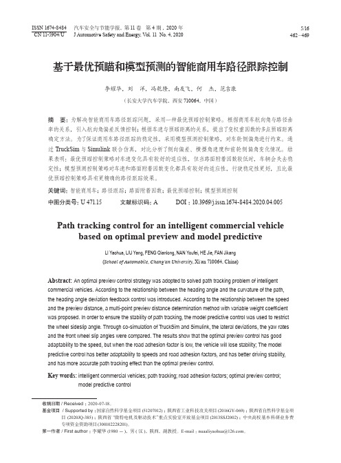
J Automotive Safety and Energy, Vol. 11 No. 4, 2020462—469基于最优预瞄和模型预测的智能商用车路径跟踪控制李耀华,刘 洋,冯乾隆,南友飞,何 杰,范吉康(长安大学汽车学院,西安710064,中国)摘要:为解决智能商用车路径跟踪问题,采用一种最优预瞄控制策略。
根据商用车航向角与路径曲率的关系,引入航向角偏差反馈控制;根据车速与预瞄距离的关系,提出了变权重因数的多点预瞄距离确定方法。
为了保证商用车路径跟踪的稳定性,采用模型预测控制策略,对车轮侧偏角进行约束。
通过TruckSim与Simulink联合仿真,对比分析了侧向偏差、横摆角速度和前轮侧偏角变化情况。
结果表明:最优预瞄控制策略对车速变化具有较好的适应性,但当路面附着因数较低时,车辆会失去稳定性;模型预测控制策略对车速和路面附着因数变化都具有较好的适应性,行驶稳定性更好,且比最优预瞄控制策略具有更精确的路径跟踪效果。
关键词:智能商用车;路径跟踪;路面附着因数;最优预瞄控制;模型预测控制中图分类号: U 471.15 文献标识码: A DOI: 10.3969/j.issn.1674-8484.2020.04.005Path tracking control for an intelligent commercial vehicle based on optimal preview and model predictiveLI Yaohua, LIU Yang, FENG Qianlong, NAN Youfei, HE Jie, FAN Jikang(School of Automobile, Chang’an University, Xi’an 710064, China)Abstract: An optimal preview control strategy was adopted to solved path tracking problem of intelligent commercial vehicles. According to the relationship between the heading angle and the curvature of the path,the heading angle deviation feedback control was introduced. According to the relationship between the speedand the preview distance, a multi-point preview distance determination method with variable weight coefficientwas proposed. In order to ensure the stability of path tracking, the model predictive control was used to restrictthe wheel sideslip angle. Through co-simulation of TruckSim and Simulink, the lateral deviations, the yaw ratesand the front wheel slip angles were compared. The results show that the optimal preview control has good adaptability to the speed, but when the road adhesion factor is low, the vehicle will lose stability; The model predictive control has better adaptability to speeds and road adhesion factors, and has better driving stability,and has more accurate path tracking effect than the optimal preview control.Key words:i ntelligent commercial vehicles; path tracking; road adhesion factors; optimal preview control;model predictive control收稿日期 / Received :2020-07-18。
Topcolor—assisted Technicolor模型对Top夸克对产生树图贡献的研究
pe i i oeceil, n hudcnie lh jr otb t n c dn et e— ee sc r nclu r c o m r rdbe o esol os r l tema nr ui s nl igt e l l et a - d tn d a oc i o i u h r v oi c
l t g tp q ak p is c o ss cin i a i o u r a r r s e to n TC2 mo e . n d1 Ke r y wo ds:o oo tpc l r—a sse e h i oo d l r e—l v lc n rb to s it d tc n c lr mo e ;te e e o ti u in;h d o old r a rnc l es i
h do o ies T eC E 5p  ̄ nds b t n e o sdi teclua o .Ii so nta tet e— ee arncldr. h T Q a o ir u o s t di ue a l i l t i m h S i nh c t n tS hw th e lvl h r
G i h n U Qn og z
( ea m n o P yis n n r a o nier g Sa gi T ahm C l g ,hnq 70 0 C ia D p r et f hs dI om t nE g ei ,hnqu ece ol eS agi 4 6 0 , h ) t ca f i n n e u n
0 引 言
目前 为止 , 准模 型 (M) 标 S 最不 清楚 的部分是 其对称 性破 缺 , 研究 电弱对 称性 破 缺机 制 是粒 子物 理 学家 当前最重 要 的任务 之一 . 理论方 面 , 人们 提 出了一些超 出标 准模 型 的新 物理模 型 , 这些 模 型在 解 释 电弱对 称 性 破缺机 制 的 同时 , 免 了标 准模 型 Hi s 部分 存在 的平 庸 性 、 自然 性 等 问题 . 各种 各样 的新 物理 模 避 g 场 g 不 在 型 中, 顶色 辅助 的人工色 ( C ) 型 _是 较 为 理想 的模 型. C T2模 l T 2模 型 不仅 合 理 的解 释 了电弱 对 称性 破 缺 机 制, 同时解 决 了重 的顶夸 克质量 问题 . 该模 型 完全 摒弃 了标准 模 型 中 的 hgs , TV能 区 引人 新 的强 相 i 场 在 e g
基于勾股模糊集理论TOPSIS的多属性决策方法及应用
基于勾股模糊集理论TOPSIS的多属性决策方法及应用基于勾股模糊集理论TOPSIS的多属性决策方法及应用摘要:多属性决策问题是现实生活中一个常见的问题,TOPSIS(Technique for Order of Preference by Similarity to Ideal Solution)是一种常用的多属性决策方法。
本文以勾股模糊集理论为基础,对TOPSIS方法进行了改进,提出了基于勾股模糊集理论TOPSIS的多属性决策方法,并通过实例应用来验证该方法的有效性。
1 引言多属性决策是在各种有限的资源约束下,通过对多种属性进行评估和权衡,最终选择出最佳的方案或决策的过程。
在现实生活中,我们经常需要面临各种各样的多属性决策问题,例如选择供应商、选租房房源、选拔员工等。
因此,研究多属性决策方法对解决实际问题具有重要意义。
2 勾股模糊集理论勾股模糊集理论是一种用于处理模糊性的数学工具。
在传统的模糊集理论中,元素与隶属度的映射关系是线性的,而在勾股模糊集理论中,元素与隶属度的映射关系是非线性的。
勾股模糊集理论包含了线性隶属度和非线性隶属度两种情况,能够更好地反映元素与隶属度之间的关系。
3 TOPSIS方法TOPSIS方法是一种常用的多属性决策方法,用于确定最优解决方案。
该方法通过计算每个方案与理想解决方案之间的相似性度量值,来排序并选择最佳方案。
其主要步骤为:(1)构建决策矩阵:将各个方案的属性值以矩阵形式表示;(2)标准化决策矩阵:通过将决策矩阵中每个元素除以其所属属性列的范数来实现;(3)计算理想解和负理想解:选择最优和最差的方案作为理想解和负理想解;(4)计算方案与理想解和负理想解的相似性度量值:使用欧氏距离或其他相似性度量方法计算;(5)计算综合评价指标:根据正理想解和负理想解之间的距离,计算综合评价指标;(6)排序并选择最佳方案:根据综合评价指标进行排序,选择最佳方案。
4 基于勾股模糊集理论TOPSIS的多属性决策方法4.1 构建勾股模糊决策矩阵:将各个方案的属性值以勾股模糊集的形式表示,并构建勾股模糊决策矩阵。
多传感器目标识别的灰色关联topsis法

多传感器目标识别的灰色关联topsis法
灰色关联 TOPSIS 法是一种基于直接灰色关联分析技术的多传感器目标识别方法,主
要用于识别大量传感器信号的异常情况,以及对传感器信号进行分类和目标识别。
这种方
法吸收了灰色关联分析的优点,如良好的去噪性能、鲁棒性和强健性,解决了传统分析方
法在信号处理方面的不足。
灰色关联TOPSIS法是基于传感器信号的各个特征进行识别的方法,它运用灰色关联
分析对传感器信号特征关联度进行识别,并通过合并和混合差异系数值,计算全局指标来
识别不同目标信号。
灰色关联TOPSIS法首先计算各个特征变量之间的相关系数,然后利
用改进型灰色关联度引入关联参数,进而计算多传感器信号特征之间的组合关联度,以便
索引不同的目标特征。
此外,还可以对各个信号特征的差异性进行合并和融合,然后根据
剂度系数,权权重进行求解,计算不同目标信号的全局指标排序,以此来确定具有最高匹
配程度的目标。
灰色关联TOPSIS法不仅可以提高识别准确性,而且具有节约资源的优势,因为它采
用了灰色关联分析和权重分配,即使对CPU进行有效利用,也能降低识别目标所需的资源,从而改善智能传感器系统的效率。
总之,灰色关联TOPSIS法是一种基于灰色关联分析的多传感器目标识别方法,通过
计算各个特征变量之间的相关系数以及关联参数,融合不同特征之间的差异性,来确定以
某个目标达到最佳匹配的全局指标。
同时,它还具有提高识别准确性和节约资源的优点,
有效地提升了智能传感器系统的效率。
基于改进的RRT^()-connect算法机械臂路径规划
随着时代的飞速发展,高度自主化的机器人在人类社会中的地位与作用越来越大。
而机械臂作为机器人的一个最主要操作部件,其运动规划问题,例如准确抓取物体,在运动中躲避障碍物等,是现在研究的热点,对其运动规划的不断深入研究是非常必要的。
机械臂的运动规划主要在高维空间中进行。
RRT (Rapidly-exploring Random Tree)算法[1]基于随机采样的规划方式,无需对构型空间的障碍物进行精确描述,同时不需要预处理,因此在高维空间被广为使用。
近些年人们对于RRT算法的研究很多,2000年Kuffner等提出RRT-connect算法[2],通过在起点与终点同时生成两棵随机树,加快了算法的收敛速度,但存在搜索路径步长较长的情况。
2002年Bruce等提出了ERRT(Extend RRT)算法[3]。
2006年Ferguson等提出DRRT (Dynamic RRT)算法[4]。
2011年Karaman和Frazzoli提出改进的RRT*算法[5],在继承传统RRT算法概率完备性的基础上,同时具备了渐进最优性,保证路径较优,但是会增加搜索时间。
2012年Islam等提出快速收敛的RRT*-smart算法[6],利用智能采样和路径优化来迫近最优解,但是路径采样点较少,使得路径棱角较大,不利于实际运用。
2013年Jordan等通过将RRT*算法进行双向搜索,提出B-RRT*算法[7],加快了搜索速度。
同年Salzman等提出在下界树LBT-RRT中连续插值的渐进优化算法[8]。
2015年Qureshi等提出在B-RRT*算法中插入智能函数提高搜索速度的IB-RRT*算法[9]。
同年Klemm等结合RRT*的渐进最优和RRT-connect的双向搜基于改进的RRT*-connect算法机械臂路径规划刘建宇,范平清上海工程技术大学机械与汽车工程学院,上海201620摘要:基于双向渐进最优的RRT*-connect算法,对高维的机械臂运动规划进行分析,从而使规划过程中的搜索路径更短,效率更高。
基于弹性模型的CT与CARTO电解剖图像的配准算法
轰‰巴盖器怒删ngR船砌2013’32(2).69~73J0um a l of B i om ed j ca l En鲥needn异ReseaI_ch…。
一。
、-,'…。
基于弹性模型的C T与C A R T O电解剖图像的配准算法术舒丽霞1△,关燕妮1,龙德勇2,喻荣辉2(1,首都医科大学附属安贞医院/北京市心肺血管疾病研究所,北京100029;2.首都医科大学附属安贞医院心内科,北京100029)摘要:提出一种全自动、高精度的cA R T o电解剖图与cT曲面配准算法。
该算法采用了由粗到精的配准策略。
粗配准部分分两步:首先采用刚体变换模型以及迭代最近点法,初次配准E A M与CT曲面;然后选择仿射变换模型,再次配准EA M与cT曲面。
在粗配准的基础上,以基于B样条的自由形变模型进一步精确配准EA M与C T曲面。
实验结果表明,相对临床常用的C a I t o—M e r ge配准软件,基于弹性模型的配准算法获得了远高于前者的E A M与C T曲面配准精度,配准效果稳定;同时算法完全自动,不需要任何手工介入。
关键词:电解割图;C T曲面;配准;C ano—M erge;B样条;FFD中图分类号:R318文献标识码:A文章编号:1672_6278(2013)02伽69m5El ast i c M odel bas ed C T and C A R T OEl ect r o—anat o皿c M ap I沁gi st r at i onS删L桶a1,G U A N Y a nI l i l,LO N G D eyon92,Y U R onghl l i2(1.B e彬愕A砌en脚删,C印豇口z胁如of‰觇巧妙,既咖,lg胁m姚旷胁。
厅hng口谢B幻od‰se Z仇s咖e,&舛,l g100029,吼i眦2.珧Por t眦川矿如一面f0∥,&彬,l g A,如趴觑印i纠,C叩矗oZ肘e d如oZ‰妇邝酊,&莎昭100029)A bst髓ct:T o pm pos e an aut om“c a nd a ccur at e C A R T0el ec t ro一曲a t oIIl i c m ap aI l d C T s udke re舀st rat i on m et hod.C oar s e t o nne st r at e gy w a s us ed.C oars e r egi st r at i on w a s di V i ded i nt0t w o st eps.Fi r st,us i ng r i gi d t r ansf0珊and I t em t i V e cl os es t Poi nt(I C P)a l-gor i t I l m,E A M and cT su血ce w e re r e舀st er ed.Then,choos i ng af f j ne t r ans f0肌,t l l ey w er e f ur t he r al i gned.B as ed on tI l e co a r se r esul t as t he i ni ti al poi n£a nd B—s pl ine f南e—f oⅡn de f oⅡna“on as t he t ra ns fom l m odel,t w o i m ages w e re6nel y r e百st ered.E xper i m ent s s how t hat ou r m et hod al i gne s E A MandC T su西ac e m uch m or e accum t el y and m or e st eadi l y tI lal l C a no—M er ge does;m e鲫w hi l e,no m anual op e r at i oni s needed du^ng出e w ho l e coar se—t o—fi II e pr oced ur e.K ey w or Il s:El ect m—anat om i c m ap;C T s ur face;re舀s t r at i on;C art o—M erge;B—s pl i ne;FFDl引言作为临床最常见的心律失常,心房颤动(房颤)的致残率和致死率很高‘1|。
car-following models based on driving strategies

基于驾驶策略的车辆跟驰模型研究及其应用前景
基于驾驶策略的跟驰模型(Car-following models based on driving strategies)是模拟车辆在道路上的行驶行为和相互作用的一种模型。
这种模型主要关注驾驶员如何根据周围环境和自身状态来选择和调整驾驶策略,以达到安全、高效地跟驰的目的。
在跟驰模型中,通常需要考虑以下几个因素:
1.驾驶员的反应时间:驾驶员从感知到前方车辆减速或加速,到自己采取相
应行动所需的时间。
这个时间取决于驾驶员的反应速度和决策能力。
2.车辆间的距离和速度差:驾驶员需要保持与前车一定的安全距离,并根据
前车的速度调整自己的速度。
这是为了防止追尾事故和保持交通流畅。
3.道路条件和交通规则:驾驶员需要根据当前道路的线形、交通标志、交通
信号等,以及遵守相应的交通规则,来选择合适的驾驶策略。
基于驾驶策略的跟驰模型可以分为两类:确定性模型和概率性模型。
确定性模型假设驾驶员的驾驶行为是确定的,可以预测的;概率性模型则考虑了驾驶员行为的随机性和不确定性。
确定性模型中最著名的就是油门-刹车线性模型(Linear Throttle-Brake Model),它假设驾驶员的油门和刹车动作是线性的,可以根据前车的速度和距离来预测下一时刻自己的速度和位置。
概率性模型中最常用的是微观跟驰模型(Microscopic Traffic Simulation Model),它考虑了驾驶员行为的随机性和不确定性,可以模拟单个车辆的运动轨迹和速度变化,从而得到整个车流的运行状态和统计特性。
JMAG脉动转矩分析brushless电机

Cogging Torque Analysis of an SPM Motor with aSkewed StatorContentsOverview (2)1 Analysis Scope (3)2 Motor Specification (3)3 Analysis Results (5)3.1 Flux Density Distribution (5)3.2 Cogging Torque (6)4 Analysis Steps (7)5 FEM Model Creation (8)5.1 Mesh Model (8)5.1.1 3D Model (8)5.1.2 Partial Model (8)5.1.3 Air Region (8)5.1.4 Winding Modeling (9)5.1.5 Mesh Generation (9)5.2 Material Properties (9)5.3 Analysis Conditions (9)5.3.1Analysis Control (9)5.3.2Step (10)5.3.3Periodic Boundary (10)5.3.4Symmetry Boundary 3D (10)5.3.5Motion (10)5.3.6Slide (10)5.3.7Electromagnetic Force and Torque Calculation (10)6 Results Display (11)6.1 Flux Density Distribution (11)6.2 Cogging torque (11)Appendix a Settings of the JMAG Analysis (12)Appendix a.1Mesh Model (12)Appendix a.2Material Properties (14)Appendix a.3Analysis Conditions (15)OverviewThe application note provides some ground for JMAG analysis. The purpose of this note is to facilitate JMAG users to gain understanding on steps and settings required for new analysis. Download the model data from JMAG Application Catalog to view the analysis model, settings and results described in the application note.The structure of the note is as follows:Section 1 Analysis ScopePresents the scope of the analysis.Section 2 Motor SpecificationSpecifies the SPM motor used for the analysis, including the geometry andspecification of the motor, material properties of the parts and the orientation of themagnet.Analysis ResultsSection 3Shows the results obtained from the analysis.Section 4 Analysis StepsExplains the analysis steps required to obtain the results presented in Section 3.Section 5 FEM Model CreationProvides some ground for the analysis settings, including the mesh model, materialproperties and the condition settings.Section 6 Results DisplayDescribes how to display the analysis results including the flux density distributionand the cogging torque waveform.AppendixShows the JMAG mesh model and the lists of the settings including materialproperties and analysis conditions. The analysis settings are identical to the settingsused on the model data available from our Website.The JMAG module(s) and the version used for the analysis are:Module TRVersion 8.41 Analysis ScopeFor motors, there is a need of reducing vibration and noise. Cogging torque is one cause of vibration and noise, so reducing cogging torque is an important issue. And one way of reducingthe cogging torque is to skew either the rotor or the stator.This note presents the use of magnetic field analysis to evaluate the cogging torque of an SPMmotor with the skewed stator.2 Motor SpecificationThe specification of the SPM motor used for the analysis is shown below.ShaftStator coreMagnetFig. 2-1 SPM motorTable 2-1SpecificationNumber of poles 4Number of slots 12Skew angle 15 degreesRotation speed 1,800 rpmShaft R:7.85mm Magnet Outer R: 11.35 mm, width: 13.5 mm, stack length: 12 mmStator core Inner R: 12.6 mm, outer R: 26.7 mm, stack length: 12 mmTable 2-2 Material propertiesPart Magnetizing properties Shaft Isotropic magnetic material: see Fig. 2-2 for BH curveMagnet Recoil Relative Permeability: 1.023,Coercive force: 7.0×10⁵ A/m Orientation: see Fig. 2-3Stator coreIsotropic magnetic steel sheet: 50H600Coil Non-magnetic material0.00.20.40.60.81.01.21.41.61.8050001000015000200002500030000Magnetic field, A/mF l u x d e n s i t y d i s t r i b u t i o n , TFig. 2-2 BH curve (shaft)Fig. 2-3 Orientation of the magnet3 Analysis ResultsThe flux density distribution and the cogging torque waveform of the SPM motor can be obtained from analysis of the SPM motor described in Section 2. Refer to Section 6 for displaying these results.3.1 Flux Density DistributionFig. 3-1 shows the flux density distribution and Fig. 3-2 shows the waveform of the flux density in the gap. The flux density waveform is the average of the flux density waveforms at 3 points that are on the linear line in the axial direction as shown in Fig. 3-1. Fig. 3-1 shows that the magnetic circuit is changed by the application of the skew. Since the skew misaligns the phases of these 3 flux density waveforms, the variation of the averaged flux density waveform is small as shown in Fig. 3-2. So it is expected that the cogging torque may be reduced by applying the skew.(Unit:T)Fig.3-10.400.420.440.460.480.500.520.540.560.580.600102030405060708090Rotation angle, degreeF l u x d e n s i t y , TFig. 3-2 Flux density waveform in the gap3.2 Cogging TorqueFig. 3-3 shows the cogging torque waveform of the SPM motor with and without the skewed stator. The peak value of cogging torque of the skewed stator is reduced by about 60 percent when compared to that of the nonskewed stator.-0.010-0.008-0.006-0.004-0.0020.0000.0020.0040.0060.0080.010010203040506Rotation angle, degreeT o r q u e , N mFig. 3-3 Cogging torque waveform4 Analysis StepsTo evaluate the cogging torque of the SPM motor with skewed stator, the transient response magnetic field analysis is used.For this analysis, FEM model is created using 3D CAD data.Two different FEM models, CAD data with skew and CAD data without skew, are used for the analysis; however, the analysis conditions and analysis steps are the same for both FEM models.The details of the analysis are provided in the following sections.STEP1:Create an FEM modelSTEP2:Run magnetic field analysisSTEP3:Evaluate the results5 FEM Model CreationAn FEM model is required to run magnetic field analysis.The FEM model is composed of a mesh model, material properties, and analysis conditions. The settings required for the cogging torque calculation are as follows.5.1 Mesh ModelSome specific points to note on the creation of a mesh model are provided next. Refer to “Appendix a.1 Mesh Model” for the list of the meshing parameters used for the analysis.5.1.1 3D Model3D model can be used when the stator core is skewed and the magnetic circuit has the 3D structure.5.1.2 Partial ModelA quarter model can be used when the motor geometry has a periodicity of 90 degrees, and the magnetic field reverses every 90 degrees.The analysis can be run efficiently with the partial model because it can reduce the time for data creation and calculation as well as the load to the computer.The partial model requires the periodic boundary condition settings. For details, see “5.3.3 Periodic Boundary”.5.1.3 Air RegionWhen the magnetic circuit is closed within the rotor and the stator, the radius of the mesh model including the air region can be set to 1.25 times the radius of the motor.The air region is required even if the magnetic circuit is closed within the motor because of the flux leakage caused by the saturation. The adequate size of the air region is 1.05 to 2.5 times the radius of the stator, and the optimum value varies with state of the saturation.The symmetry boundary condition needs to be specified on the circumference of the mesh model, assuming that the magnetic field does not leak out of the air region. For details, see “5.3.4 Symmetry Boundary 3D”.5.1.4 Winding ModelingTo simplify the model of the coil end, a solid model of the stator coil is created as the length of the stator coil is to be 2.0 times the thickness of the motor.Since the effect of magnetic saturation at the stator core where flux flows is considered small, almost all of the interlinkage flux through the coil seems to flow into the stator core. Even if the model of the coil end is simplified, there is no impact on the current flow. The adequate size of the solid model is 1.25 to 2.5 times the thickness of the alternator, and the optimum value varies with the state of the saturation.5.1.5 Mesh GenerationAs the shaft and the magnet have the rotation motion, the cylindrical slide mesh option can be used to generate the mesh in the gap between the stator and the rotor. The size of elements in the gap varies with the motor geometry.To analyze the amplitude and the periodicity of cogging torque accurately, the mesh should be divided in circumferential direction. For this analysis, the number of divisions in the circumferential direction is set to 90 in order to divide one period (30 degrees) of cogging torque into 30. The number of divisions in the radial direction is set to 3.To generate the fine mesh at the gap, the size of elements should be set for the solid face facing the gap.5.2 Material PropertiesThe material properties of the parts vary with the motor. For this analysis, the values are specified with reference to the material properties as described in Table 2-2. For the settings, see “Appendix a.2 Material Properties”.5.3 Analysis ConditionsSome specific points to note on the analysis conditions are provided next. For the settings, see “Appendix a.3 Analysis Conditions”.5.3.1Analysis ControlA 3D model can be used for the analysis, as explained in “5.1.1 3D Model”. The transient response analysis should be selected when the rotation motion of the rotor is the time-varying phenomenon.When a quarter model is used for the analysis, the result conversion factor for the FEM model is set to 4.5.3.2StepThe rotor is set to rotate 1 degree per step in this analysis, and the time interval must be specified for each rotation speed. When the analysis is run for the mechanical angle of 60 degrees, the number of steps is set to 61 and the time interval is set to 1/10800 seconds.5.3.3Periodic BoundaryThe periodic boundary must be specified when a partial model is used, as explained in “5.1.2 Partial Model”. The anti periodic boundary is set to 90 degrees, since the model geometry has a periodicity of 90 degrees in the circumferential direction and the direction of the magnetic field reverses every 90 degrees.When the center of the rotation is the origin and the rotation axis is Z-axis, a point on potation axis is set to (0,0,0) and the direction of rotation axis is set to (X,Y,Z)=(0,0,1).5.3.4Symmetry Boundary 3DThe symmetry boundary must be set on the circumference of the mesh model, assuming that the magnetic field does not leak out of the air region. The flux flows parallel and the current flows perpendicular to the face where this condition has been specified.5.3.5MotionThe motion condition should be set on the rotating parts including the shaft and the magnet. When the center of the rotation is the origin and the rotation axis is Z-axis which rotates in a counterclockwise direction, a point on rotation axis is set to (0,0,0) and the direction of rotation axis is set to (VX,VY,VZ)=(0,0,1). The rotation speeds is set to the constant with 1800 rpm according to the specification described in Table 2-1.5.3.6SlideThe cylindrical slide mesh option can be used to generate the mesh, as explained in “5.1.5 Mesh Generation”. With this option, the slide condition would be set automatically during the mesh generation.5.3.7 Electromagnetic Force and Torque CalculationFor this analysis, this condition is set on the shaft and the magnet to calculate the torque generated in the rotating parts. The nodal force method is used when the condition is set on the magnetic material.6 Results DisplayThe followings instruct how to view the analysis results described in Section 3.6.1 Flux Density DistributionWhen magnetic field analysis is complete, the results are exported to the PLOT file.In this note, the flux density distribution is displayed in contour. The flux density waveform is displayed in the graph using the spreadsheet software.To display the flux density distribution as shown in Fig. 3-1, open the PLOT file, and select Results > Magnetic Flux Density > Contour > Magnetic Flux Density.To display the flux density waveform as shown in Fig. 3-2, open the PLOT file, and select elements in the gap on the rotor side. To obtain the averaged flux density waveform in the axis direction, select three points on the straight line. Selected points are shown in Fig. 6-1. Then, select Results > Magnetic Flux Density > Table > Magnetic Flux Density > Step Range: All > Export File. Values of the flux density at each step are exported. Fig. 3-2 shows the averaged flux density waveform of three points obtained using the spreadsheet software. In this note, the flux density with and without skew are displayed in one graph.Fig. 6-1Air region on the rotor side (●: selected elements)6.2 Cogging torqueWhen magnetic field analysis is complete, the results are exported to the PLOT file.In this note, the torque generated at the rotating parts is displayed by the history graph.To create the history graph as shown in Fig. 3-3, open the PLOT files, and select Results > Torque (Electromagnetic force) > History, and then select Option > Show Rotation Angle. Change the label of X-axis from ‘Time’ to ‘Rotation angle’ to display cogging torque.AppendixAppendix a Settings of the JMAG AnalysisThe mesh model and the settings including the material properties and the analysis conditions are shown in the following sections. The settings are the identical to the model data ”JAC024SPM-Skew-01e.jcf” and ”JAC024SPM-noSkew-01e.jcf”, which can be downloaded from “Cogging Torque Analysis of an SPM Motor with a Skewed Stator” in online JMAG Application Catalog.Appendix a.1Mesh ModelThe mesh model used for the analysis is shown in Fig. a-1 and Fig. a-2. The settings for the mesh generation are listed in Table a-1. For the ground for the settings, see “5.1 Mesh Model”.Fig. a-1Mesh model with skew (number of elements: 224,053)Fig. a-2Mesh model without skew (number of elements: 227,419)Table a-1Automatic mesh generationParameter ValueMesh Type Cylindrical SlideMeshType of Input Data SolidNumber of division alongRadial Direction3Number of Division along Circumferential Direction 90Cylindrical Slide MeshParametersScale of Air Region in Vertical Direction 1 Scale of Air Region 1.25 Air Region Element Size (mm) 5 Shaft Element Size (mm) 2.0Magnet Element Size (mm) 1.0Stator core Element Size (mm) 1.0Coil Element Size (mm) 3.0 PartsSolid face ofthe gapElement Size (mm) 0.4Appendix a.2Material PropertiesThe material properties specified on the model are listed on Table a-2. For the ground for thesettings, see “5.2 Material Properties”.Table a-2Material propertiesPart Parameter Value Type Isotropic Magnetic MaterialType NonlinearMaterial(B-H) Shaft MagnetizingProperties Point Sequence See Fig. 2-3Type MagnetType LinearMaterialMagnetizing Properties Recoil RelativePermeability1.023Type ParallelPattern(Circular Direction) Number of Poles 4Starting Position theta 0 (deg) 45X-coordinate (m) 0Y-coordinate (m) 0MagnetizationDirectionCenterPointZ-coordinate (m) 0MagnetCoercive Force (A/m) 700,000Type Isotropic Magnetic Steel SheetType NipponSteel(MaterialDatabase) Stator core MagnetizingProperties Point Sequence 50H600U phase coil Type CoilV phase coil Type CoilW phase coil Type CoilAppendix a.3 Analysis ConditionsThe settings of the analysis conditions and the circuit conditions are listed in Table a-3 and Table a-4. For the ground for the settings, see “5.3 Analysis Conditions”. The conditions highlighted in bold are specific to the motor, so there is no need to change the settings when the analysis content is changed. The conditions not highlighted in bold can be modified freely.Table a-3 Analysis conditionsCondition Parameter ValueType3D Transient Response Analysis Analysis Control (see 5.3.1) Conversion Factor Periodic Boundary4 Number of Steps61 Step Regular IntervalInitial Value (sec)0 End Point (sec) 1 Step (see 5.3.2)Regular IntervalNumber of Division 10,800TargetXZ plane of mesh modelBoundary Anti-Periodic Boundary Periodicity RotationalA Point on Rotation Axis X,Y , Z coordinate (m) (0,0,0) Direction of Rotation Axis X,Y , Z(0,0,1) Periodic Boundary (see 5.3.3)Angle (deg)90Symmetry Boundary 3D (see 5.3.4) TargetOuter circumference of the mesh modelTarget Shaft, magnet Type RotationA Point on Rotation Axis X,Y and Z coordinate (m)(0,0,0) Direction of Rotation AxisVX,VY and VZ(0,0,1)Definition DisplacementMethod Constant: 1800rpmMotion (see 5.3.5)Parameter Velocity Region Face (Edge) 1 Gap edge on rotor side Slide (see 5.3.6)TargetRegion Face (Edge) 2Gap edge on stator sideTable a-4Analysis conditionsCondition Parameter Value Target Shaft,magnetA Point on TorqueAxisX,Y,Z coordinate (m) (0,0,0)Torque Axis Vector X,Y, Z (0,0,1)Electromagnetic Forceand Torque Calculation(see 5.3.7)Method NodalForceURL http://www.jri.co.jp/pro-eng/jmag/support/e/catalog/Technical SupportJRI Solutions, Ltd.Engineering Technology DivisionJMAG Support Teamjmag-support@sci.jri-sol.co.jporDistributor in your countryJMAG Application Note Copyright(C) 2006-2007 JRI Solutions, Ltd. All Rights Reserved.。
traffic jam的英语作文

Traffic jams are a common phenomenon in many urban areas around the world, causing inconvenience and frustration for commuters.Heres a detailed essay on the topic:Title:The Plight of Traffic JamsIntroduction:The modern city is a marvel of human ingenuity,yet it is not without its challenges.One such challenge is the traffic jam,a daily ordeal for many city dwellers.This essay aims to explore the causes,impacts,and potential solutions to the traffic congestion that plagues our roads.Causes of Traffic Jams:1.Population Growth:As cities expand,so does their population.More people mean more vehicles on the road,leading to increased traffic.2.Urban Sprawl:The expansion of cities into suburban areas often results in longer commutes,as people travel from the outskirts to the city center for work.3.Inefficient Public Transportation:Inadequate public transport systems push more people to use private vehicles,exacerbating congestion.4.Poor Road Infrastructure:Narrow roads,lack of maintenance,and insufficient road networks contribute to traffic bottlenecks.5.Accidents and Incidents:Even a minor accident can cause a ripple effect,slowing down traffic for miles around.Impacts of Traffic Jams:1.Environmental Impact:Idle vehicles emit more pollutants,contributing to air pollution and climate change.2.Economic Cost:Traffic congestion leads to lost productivity,as workers spend hours stuck in traffic instead of being at their workplaces.3.Health Issues:Prolonged exposure to traffic pollution can lead to respiratory problems and other health issues.4.Stress and Mental Health:The frustration of being stuck in traffic can lead to increased stress levels and mental health issues.5.Accidents:Congested roads increase the likelihood of accidents due to the high density of vehicles.Potential Solutions:1.Improving Public Transportation:Investing in better,more reliable public transport can reduce the number of vehicles on the road.2.Encouraging Carpooling and Cycling:Promoting carpooling and cycling can decrease the number of individual vehicles.3.Implementing Traffic Management Systems:Advanced traffic management systems can optimize traffic flow and reduce congestion.4.Expanding Road Infrastructure:Building more roads and improving existing ones can accommodate higher traffic volumes.5.Adopting Smart City Technologies:Utilizing IoT and AI technologies for traffic prediction and management can alleviate congestion.Conclusion:Traffic jams are a complex issue with no single solution.It requires a multifaceted approach involving urban planning,infrastructure development,and behavioral changes among commuters.By addressing the root causes and implementing innovative solutions, we can hope to reduce the frequency and severity of traffic jams,making our cities more livable and our roads safer.Recommendations:Encourage the use of public transport through subsidies and improved services. Implement congestion pricing to deter the use of private vehicles during peak hours. Develop green spaces and pedestrianfriendly zones to reduce reliance on cars for short distances.Educate the public on the benefits of ecofriendly commuting options.In conclusion,while traffic jams may seem like an insurmountable problem,with concerted effort and innovative thinking,we can work towards a future where our roads are less congested and our cities more efficient.。
基于背景学习与方向预测的车辆图像跟踪
文 章 编 号 :6 14 2 (0 10 - 4 -8 17 —2 9 2 1 )2 0 20 0
基于 背 景 学 习与方 向预测 的车 辆 图像 跟 踪
梁 忠伟 2,钟 志聪
(. 1 广州大学 机械与电气工程学 院, 广东 广州 50 0 ;. 106 2 华南理工大学 a 机械与汽车工程学 院 .
LAN G o g we I Zh n — i 一.ZHONG it n Zh — o g
( c olቤተ መጻሕፍቲ ባይዱf c a i l Ee tcl n i eig G a gh u U i r t, u gh u50 0 , hn ; 1 S h h nc & l r a E gn r , u n zo nv s yG a zo 1 6 C i o Me a ci e n ei n 0 a
目标 的定 位 及 速 度 确 定 , 结合 方 向预 测 算 子 对 车 辆 行 驶 矢 量 进行 预 测 , 而 实现 目标 车辆 的 图 像 跟 踪 .跟 踪 实 进
验 及 性 能 比较 证 明本 方 法 可 获 得 准 确 稳 定 的运 动 车辆 跟 踪 结 果 , 为运 动 目标 的 图像 监 控 研 究提 供 了新 的 思路 .
M t l tr l , o t C iaU iesy o T c n lg , u n z o 6 0, hn ) ea i Ma i s S uh hn nv r t f e h o y G a gh u5 4 C i lc ea i o 1 0 a
Ab t a t s r c :Fo h u p s fmo i g tr e ’ ee tn rt e p r o e o v n a g t Sd t ci g,a ma e ta k n to a e n te c a gn a tr n i g r c i g meh d b s d o h h n i g fco o ee e c c g o n e r n n h ie t n p e c i p r tri r s n e fr f r n e ba k r u d l anig a d t e d r ci rdit o ng o e ao sp e e td. Th ih—p e vn e e h g s e d mo i g v —
国际滑翔伞基地英语作文

The International Paragliding Base is a haven for adventure seekers and paragliding enthusiasts from all around the globe.Located amidst breathtaking landscapes,it offers an unparalleled experience of soaring through the skies with the wind as your guide.Facilities at the BaseThe base is equipped with stateoftheart facilities to ensure a safe and enjoyable paragliding experience.It includes:Training Grounds:For beginners to learn the basics of paragliding under the supervision of certified instructors.Launching Platforms:Strategically positioned to take advantage of the regions wind patterns,providing optimal conditions for takeoff.Landing Zones:Spacious and wellmaintained areas designed to accommodate safe landings.Paragliding ExperiencesVisitors can choose from a variety of paragliding experiences tailored to different skill levels and preferences:Introductory Flights:For firsttimers,these flights are short and gentle,offering a taste of the thrill without overwhelming the participant.Intermediate Tours:Longer flights that take pilots over scenic routes,providing a more challenging and rewarding experience.Advanced Adventures:For experienced paragliders,these flights involve navigating more complex terrains and longer durations in the air.Safety MeasuresSafety is paramount at the International Paragliding Base.All flights are conducted under strict safety protocols,including:PreFlight Briefings:Detailed instructions on safety procedures and flight plans. Equipment Checks:Regular maintenance and inspections of all paragliding gear to ensure optimal performance and safety.Weather Monitoring:Continuous assessment of weather conditions to prevent any risky flights.Accommodations and AmenitiesTo make the stay comfortable and enjoyable,the base provides:Accommodation Options:From budgetfriendly hostels to luxurious lodges,catering tovarious preferences and budgets.Dining Facilities:A variety of restaurants and cafes offering local and international cuisine.Recreational Activities:Besides paragliding,the base also offers other outdoor activities such as hiking,mountain biking,and rock climbing.Community and EventsThe International Paragliding Base fosters a vibrant community of paragliders and hosts several events throughout the year:Paragliding Competitions:Attracting professional paragliders from around the world to compete in various categories.Cultural Festivals:Celebrating the local culture with music,dance,and traditional food. Workshops and Seminars:Educational events for paragliders to enhance their skills and knowledge.ConclusionThe International Paragliding Base is more than just a place for adventure its a community that brings together people from different backgrounds with a shared passion for flight.Whether youre a seasoned paraglider or a curious beginner,this base offers an unforgettable experience that will leave you with a new perspective on the world from the skies above.。
基于TOPSIS模型的山区道路敏感性评价

-(;"-($ .#'''!%'%'#"% .''"' .'$
'()* +DPPBQK5PCJM7JO;HM:JO
,;9"% SJ:J<YJM%'%'
WX (+Q!&!YZC[A\]^_`ab
ü,-./×01
! Û*É}y"Û §¤ì '&''%"#
¡¢ !\]7_`¾a×þ;¾1@R+*+ £¤¥¦; !A)"%9$%! -§¨©ª !_
!/<>5;5@5;= )@67D6;58<8?T8D<;65<*86H>:6>/H8<(+Q!&!T8H/7
UA68 (5/>8<B !D<CD78<B '6<B Z538<B ! =JYJK6JCJ;M;E;VK:PESKOPOCJMRMJNJBCK;B /JBCJM"+DKeKPXDHPBV'&''%"" =JYJK# #2>;360;& 1PdKBVCFLK:PE<;HBCPKB;HOPMJPOKB =JYJKRM;NKB:JPOCDJMJOJPM:D ;YTJ:C" G;HMKBIK:PC;MOKB:EHIKBVNPE]
. All EJRFiYg;ChC;<tsGEPCBRJeOOs:e;<rLvMJeDJdB.OKNJKBIJQ" B;M<PEKXJI NJVJCPCK;B KBIJQ" O;KEYHEd IJBOKCFPBI VJ;E;VK:PEDPXPMI DKIIJB
Learning Visual Maps Correlated with Other Sensors and Motor Systems

References
1] H. Bauer and K. Pawelzik. Quantifying the neighborhood preservation of self-organizing feature maps. IEEE Transactions on Neural Networks, 3(4):570{579, 1992. 2] M. Brainard and E. Knudsen. Experience-dependent plasticity in the inferior colliculus: A site for visual calibration of the neural representation of auditory space in the barn owl. The Journal of Neuroscience, 13(11):4589{4608, 1993. 3] M. Brainard and E. Knudsen. Dynamics of visually guided auditory plasticity in the optic tectum of the barn owl. Journal of Neurophysiology, 73(2):595{614, 1995. 4] R. Durbin and G. Mitchison. A dimension reduction framework for understanding cortical maps. Nature, 343(6259):644{647, 1990. 5] M. Hassoun. Fundamentals of Arti cial Neural Networks. MIT Press, Cambridge, MA, 1995. 6] S. Haykin. Neural Networks: A Comprehensive Foundation. Macmillan College Publishing Company, New York, NY, 1994. 7] T. Kohonen. Self-organized formation of topologically correct feature maps. Biological Cybernetics, 43:59{69, 1982. 8] K. Miller. Correlation-based models of neural development. In M. Gluck and D. Rumelhart (eds.), editors, Neuroscience and Connectionist Theory, pages 267{353. Lawrence Erlbaum Associates, Hillsdale, NJ, 1990. 9] K. Miller, J. Keller, , and M. Stryker. Ocular dominance column development: Analysis and simulation. Science, 245:605{615, 1989. 10] K. Miller and M. Stryker. The Development of Ocular Dominance Columns: Mechanisms and Models. MIT Press, Boston, MA, 1990. 11] D. Mitchell and B. Timney. Postnatal Development of Function in the Mammalian Visual System. ??, ??, 1984. 12] K. Obermayer, H. Ritter, , and K. Schulten. A principle for the formation of the spatial structure of cortical feature maps. Proceedings of the National Academy of Science USA, 87:8345{8349, 1990. 13] H. Ritter and K. Schulten. Kohonen's self-organizing maps: Exploring their computational capabilites. In Proceedings of the IEEE International Conference on Neural Networks, volume 1, pages 109{116, San Diego, CA, 1988.
车辆跟驰行为建模的回顾与展望_王殿海
从跟驰模型推导模型得到了 GM 模型 进 行 积 分 , 从而在交通流 G r e e n b e r g 宏观流量 -速 度 关 系 模 型 , 微观模型和宏观理论之 间 建 立 起 联 系 。1 文 9 5 9 年, , [ , [ 这3篇论文共同获得运筹学 献[ 1 1] 1 2] 1 3] 开创 了 微 观 交 通 流 理 论 的 研 究 。 接 L a n c h e s t e r奖 , [ 1 4] 着, G a z i s等 进一 步 提 出 了 GM 模 型 的 一 般 表 达 式, 并通过改变不同的参数得到各种宏观流量 -密度
211刺激反应类模型刺激反应框架是最基本的跟驰行为建模框架它将前导车对驾驶人的作用表示为一种刺激st将驾驶人的感知能力作为其对刺激的一种敏感系数se将驾驶人的反应re表示为跟驰车的运动行为如式1所示resest1刺激反应框架是最经典的跟驰行为建模思想集中体现了跟驰行为中许多本质特征
第2 5卷 第1期 2 0 1 2年1月
刺激 -反应的模式提出了 GM 模型的原型 , 建立了跟 并 驰车加速度与前后 车 相 对 速 度 之 间 的 关 系 模 型 , 通过在 GM 试 车 场 获 取 的 跟 驰 行 为 数 据 来 标 定 和 其对跟驰数据获取方法的试验 , 开创 验证理论模型 ,先 河 。 此 后 , H e r m a n
收稿日期 : 2 0 1 1 0 5 2 1 - - “ ) ; ) 基金项目 : 国家高技术研究发展计划 ( 八六三 ” 计划 ) 项目 ( 国家自然科学基金项目 ( 2 0 1 1 AA 1 1 0 3 0 4 7 0 9 7 1 0 5 3 , : 。 作者简介 : 王殿海 ( 男, 吉林大安人 , 教授 , 博士研究生导师 , 工学博士 , 博士后 , 1 9 6 2 E-m a i l w a n d i a n h a i u. e d u. c n -) @z g j
基于分形几何边界提取的图像跟踪方法

基于分形几何边界提取的图像跟踪方法
王艳玲;张玘;罗诗途
【期刊名称】《光电子技术与信息》
【年(卷),期】2005(018)006
【摘要】为了满足现代武器装备对图像跟踪系统的实时性和跟踪可靠性的双重要求,针对武器装备所跟踪目标的特点,将基于分形几何的边界提取方法用于图像跟踪系统,提出了一种基于运动区域和边界图像的目标跟踪方案.文中的边界提取方法不仅能提取出目标的轮廓,还能较好地保留其内部细节,这样通过模板匹配得到的最佳匹配位置更加可靠.同时,基于运动区域的边界提取,大大减少了计算量,尤其是对于远景的目标跟踪.此外,在利用边界图像进行匹配的基础上,采用了自适应模板更新策略,目的是尽可能地克服形变、光照等影响,使跟踪过程准确可靠.仿真实验表明,该方法运算量小,能满足武器装备实时性的要求,并行之有效.
【总页数】4页(P49-52)
【作者】王艳玲;张玘;罗诗途
【作者单位】国防科技大学机电工程与自动化学院湖南长沙 410073;国防科技大学机电工程与自动化学院湖南长沙 410073;国防科技大学机电工程与自动化学院湖南长沙 410073
【正文语种】中文
【中图分类】TN911.73
【相关文献】
1.基于声图像的海底地形边界提取算法 [J], 王媛媛;郭延恩;施国全;韦俊霞;夏顺仁
2.利用模糊边界提取算法实现医学图像边界提取 [J], 顾晖;程晨;梁惺彦
3.基于图像边界提取的果园作业机器人自主导航系统 [J], 叶小琴;陈超
4.基于分形几何边界提取的图像跟踪方法 [J], 罗诗途;王艳玲;罗飞路;孙宏亮
5.基于改进蚁群算法的医学图像边界提取 [J], 陈超
因版权原因,仅展示原文概要,查看原文内容请购买。
- 1、下载文档前请自行甄别文档内容的完整性,平台不提供额外的编辑、内容补充、找答案等附加服务。
- 2、"仅部分预览"的文档,不可在线预览部分如存在完整性等问题,可反馈申请退款(可完整预览的文档不适用该条件!)。
- 3、如文档侵犯您的权益,请联系客服反馈,我们会尽快为您处理(人工客服工作时间:9:00-18:30)。
Modeling cortical maps with TopographicaJames A.Bednar a,Yoonsuck Choe b,Judah De Paula a,Risto Miikkulainen a,Jefferson Provost a,and Tal Tversky aa Department of Computer Sciences,The University of Texas at Austin,Austin,TX78712{jbednar,tal,jp,judah,risto}@b Department of Computer Science,Texas A&M University,TAMU3112,College Station,TX77843choe@AbstractThe biological function of cortical neurons can often be understood only in the context of large,highly interconnected networks.These networks typically form two-dimensional topographic maps,such as the retinotopic maps in the visual putational simulations of these areas have led to valuable insights about how cortical topography develops and functions,but further progress is difficult because appropriate simulation tools are not available.This paper introduces the freely available Topographica map-level simulator,currently under development at the University of Texas at Austin.Topographica is designed to make large-scale,detailed models practical.The goal is to allow neuroscientists and compu-tational scientists to understand how topographic maps and their connections organize and operate.This understanding will be crucial for integrating experimental observations into a comprehensive theory of cortical function.Key words:simulation tools,cortical modeling,topographic maps,self-organization,development1IntroductionMuch of the cortex of mammals can be partitioned into topographic maps[8,13].These maps contain systematic two-dimensional representations of features relevant to sensory and motor processing,such as retinal position,sound frequency,line orientation,and motion direction [5,9,14].Understanding the development and function of topographic maps is crucial for un-derstanding brain function,and will require integrating large-scale experimental imaging results with single-unit studies of individual neurons and their connections.Computational simulations have proven to be a powerful tool in this endeavor.In a simulation, it is possible to explore how topographic maps can emerge from the behavior of single neu-rons,both during development and during perceptual and motor processing in the adult.(For a review of this class of models,see[12].)However,the models to date have been limited in size and scope because existing simulation tools do not provide specific support for biologically realistic,densely interconnected topographic maps.Existing biological neural simulators,such as NEURON[7]and GENESIS[6],primarily focus on detailed studies of individual neuronsPhotoreceptors ON-cellsOFF-cellsOFF-cellsON-cellsLGNV1GangliaRetinalHigher visual areasFig.1.Topographica models.This figure shows a sample Topograph-ica model of the early visual system [3,4].In Topographica ,models are composed of interconnected sheets of neurons.Each visual area in this model is represented by one or more sheets.For instance,the eye is rep-resented by three sheets:a sheet rep-resenting an array of photoreceptors,plus two sheets representing retinal ganglion cells.Each of the sheets can be coarse or detailed,plastic or fixed,as needed for a particular study.Sheets are connected to other sheets,and units within each sheet can be connected using lateral con-nections.For one cell in each sheet in the figure,sample connections are shown,including lateral connections in V1and higher areas.Similar mod-els can be used for topographic maps in somatosensory,auditory,and mo-tor cortex.or very small networks of them.Tools for simulating large populations of abstract units,such as PDP++[10]and Matlab (),focus on cognitive science and engineer-ing applications,rather than models of cortical areas.As a result,current simulators also lack specific support for measuring topographic map structure or generating input patterns at the topographic map level.This paper introduces the Topographica map-level simulator,which is designed to make it prac-tical to simulate large-scale,detailed models of topographic maps.Topographica is designed to complement the existing low-level and abstract simulators,focusing on biologically realistic networks of tens of thousands of neurons,forming topographic maps containing millions or tens of millions of connections.Topographica is being developed at the University of Texas at Austin as part of the Human Brain Project of the National Institutes of Mental Health.Topographica is an open source project,and binaries and source code will be freely available through the in-ternet at .In the sections below,we describe the models and modeling approaches supported by Topographica ,how the simulator is implemented,and how it can be used to advance the field of computational neuroscience.2Scope and designFigure 1illustrates the types of models supported by Topographica .The models focus on to-pographic maps in any two-dimensional cortical or subcortical region,such as visual,auditory,somatosensory,proprioceptive,and motor maps.Typically,models will include multiple re-gions,such as an auditory or visual processing pathway,and simulate a large enough area to allow the organization and function of each map to be studied.The external environment must also be simulated,including playback of visual images,audio recordings,and test patterns. Current models typically include only a primary sensory area with a simplified version of an input pathway,but larger scale models will be crucial for understanding phenomena such as object perception,scene segmentation,speech processing,and motor control.Topographica is intended to support the development of such models.To make it practical to model topographic maps at this large scale,the fundamental unit in the simulator is a two-dimensional sheet of neurons,rather than a neuron or a part of a neuron. Conceptually,a sheet is a continuous,two-dimensional area(as in[1,11]),which is typically approximated by afinite array of neurons.This approach is crucial to the simulator design, because it allows user parameters,model specifications,and interfaces to be independent of the details of how each sheet is implemented.As a result,the user can easily trade off between simulation detail and computational require-ments,depending on the specific phenomena under study in a given simulator run.(See[2]for more details on model scaling.)If enough computational power and experimental measurements are available,models can be simulated at full scale,with as many neurons and connections as in the animal system being studied.More typically,a less-dense approximation will be used, requiring only ordinary PC workstations.Because the same model specifications and parame-ters can be used in each case,switching between levels of analysis does not require extensive parameter tuning or debugging as would be required in neuron-level or engineering-oriented simulators.For most simulations,the individual neuron models within sheets can be implemented at a high level,consisting of single-compartmentfiring-rate or integrate-and-fire units.More de-tailed neuron models can also be used,when required for experimental validation or to simulate specific phenomena.These models will be implemented using interfaces to existing low-level simulators such as NEURON and GENESIS.3ImplementationTopographica consists of a graphical user interface(GUI),scripting language,and libraries of models,analysis routines,and visualizations.The model library consists of predefined types of sheets,connections,neuron models,and learning rules,and can be extended with user-defined components.These building blocks are combined into a model using the GUI and(when neces-sary)the script language.The analysis and visualization libraries include statistical tests and plotting capabilities geared towards large,two-dimensional areas.They also focus on data displays that can be compared with experimental results,such as optical imaging recordings,for validating models and for generating predictions.Figure2shows examples of the visualization types currently supported. Thisfigure is a screenshot from a prototype version of Topographica,available for download at .To allow large models to be executed quickly,the numerically intensive portions of the simulatorFig.2.Software screenshot.This image shows a sample session of a prototype version of Topographica that is available freely at .Here the user is studying the behavior of an orienta-tion map in the primary visual cortex(V1),using a model similar to the one depicted infigure1.The window at the bottom labeled“Orientation”shows the self-organized orientation map and the orientation selectivity in V1.The windows labeled“Activity”show a sample visual image on the left,along with the responses of the retinal ganglia and V1(labeled“Primary”).The input patterns were generated using the“Test pattern parameters”dialog at the left.The window labeled“Weights”shows the strengths of the connections to one neuron in V1.This neuron has afferent receptivefields in the ganglia and lateral receptivefields within V1.The afferent weights for an8×8and4×4sampling of the V1neurons are shown in the“Weights Array”windows on the right;most neurons are selective for Gabor-like patches of oriented lines.The lateral connections for an8×8sampling of neurons are shown in the“Weights Array”window at the lower left;neurons tend to connect to their immediate neighbors and to distant neurons of the same orientation.This type of large-scale analysis is difficult with existing simulators,but Topographica is well suited for it.See for a color version of thisfigure.are implemented in C++.Equally important,however,is that prototyping be fast andflexible, and that new architectures and other extensions be easy to explore and test.Although C++allows thefine control over machine resources that is necessary for peak performance,it is difficult towrite,debug and maintain complex systems in C++.To provideflexibility,the bulk of the simulator is implemented in the Python scripting language. Python is an interactive high-level language that allows rapid software development and interac-tive debugging,and includes a wide variety of software libraries for tasks such as data analysis, statistical measurements,and visualization.Unlike the script languages typically included in simulators,Python is a complete,well-defined,mature language with a strong user base.As a result,it enjoys strong support outside of thefield of computational neuroscience,which pro-vides much greaterflexibility for users as well as making the task of future maintenance easier. Thefirst full release of Topographica is scheduled for mid-2004,and will include support for Linux,Microsoft Windows,and Macintosh OS X platforms.This release focuses on support for models of vision,but many of the primitives are also usable for auditory and somatosensory models.Included areflexible routines for generating visual inputs(based on geometric pat-terns,mathematical functions,and photographic images),and general-purpose mechanisms for measuring maps of visual stimulus preference,such as orientation,ocular dominance,motion direction,and spatial frequency maps.4Future researchUsing the tools provided by Topographica,we expect that neuroscientists and computational researchers will be able to answer many of the outstanding research questions about topographic maps,including what roles environmental and intrinsic cues play in map development,and what computations they perform in the adult.Other current research topics include understanding how object segmentation,grouping,and recognition are implemented in maps,and how feedback from higher areas and visual attention affect lower level responses.The simulator is designed throughout to be general and extensible,and so it will also be able to address new research questions that arise from future experimental work.Several releases of Topographica are planned over the next few years,including user-contributed extensions and models.An online repository will also be set up for user contributions,so that researchers can share code and models.The overall goal is to work towards a common under-standing of how topographic maps develop and function.5ConclusionThe Topographica simulatorfills an important gap between existing software for detailed mod-els of individual neurons,and software for abstract models of cognitive processes.The simulator focuses on models formulated at the topographic map level,which is crucial for understanding brain function.We believe this shared,extensible tool will be highly useful for the community of researchers working to understand the large-scale structure and function of the cortex. AcknowledgmentsSupported in part by the National Institutes of Mental Health under Human Brain Project grant 1R01-MH66991,and by the National Science Foundation under grant IIS-9811478.References[1]Amari,S.-I.(1980).Topographic organization of nervefields.Bulletin of MathematicalBiology,42:339–364.[2]Bednar,J.A.,Kelkar,A.,and Miikkulainen,R.(2004).Scaling self-organizing maps tomodel large cortical networks.Neuroinformatics.In press.[3]Bednar,J.A.,and Miikkulainen,R.(2003).Learning innate face preferences.NeuralComputation,15(7):1525–1557.[4]Bednar,J.A.,and Miikkulainen,R.(2003).Self-organization of spatiotemporal recep-tivefields and laterally connected direction and orientation maps.Neurocomputing,52–54:473–480.[5]Blasdel,G.G.(1992).Orientation selectivity,preference,and continuity in monkey striatecortex.Journal of Neuroscience,12:3139–3161.[6]Bower,J.M.,and Beeman,D.(1998).The Book of GENESIS:Exploring Realistic NeuralModels with the GEneral NEural SImulation System.Santa Clara,CA:Telos.[7]Hines,M.L.,and Carnevale,N.T.(1997).The NEURON simulation environment.NeuralComputation,9:1179–1209.[8]Kaas,J.H.(1997).Theories of visual cortex organization in primates.Cerebral Cortex,12:91–125.[9]Merzenich,M.M.,Knight,P.L.,and Roth,G.L.(1975).Representation of cochlea withinprimary auditory cortex in the cat.Journal of Neurophysiology,38(2):231–249.[10]O’Reilly,R.C.,and Munakata,Y.(2000).Computational Explorations in Cognitive Neu-roscience:Understanding the Mind by Simulating the Brain.Cambridge,MA:MIT Press.[11]Roque Da Silva Filho,A.C.(1992).Investigation of a Generalized Version of Amari’sContinuous Model for Neural Networks.PhD thesis,University of Sussex at Brighton, Brighton,UK.[12]Swindale,N.V.(1996).The development of topography in the visual cortex:A review ofwork–Computation in Neural Systems,7:161–247.[13]Van Essen,D.C.,Lewis,J.W.,Drury,H.A.,Hadjikhani,N.,Tootell,R.B.,Bakircioglu,M.,and Miller,M.I.(2001).Mapping visual cortex in monkeys and humans using surface-based atlases.Vision Research,41(10–11):1359–1378.[14]Weliky,M.,Bosking,W.H.,and Fitzpatrick,D.(1996).A systematic map of directionpreference in primary visual cortex.Nature,379:725–728.。
