Low-density limit as a test for the models of complicated processes in the nuclei
GR5,TC4钛合金十大性能

This property of titanium shows that its yield ratio (tensile strength / yield strength) is soaring, indicating that the metallic titanium material has poor plastic deformation upon forming. Due to the titanium yield strength and elastic modulus of the ratio of fat, the resilience of titanium molding large.
Titanium is a chemically very reactive metal that reacts with many elements and compounds at elevated temperatures. Titanium suction mainly refers to elevated temperature and carbon, hydrogen, nitrogen, oxygen reaction.
6, non-magnetic, non-toxic
Titanium is non-magnetic metal that cannot be magnetized in a large magnetic field. It is non-toxic and has excellent compatibility with human tissues and blood. Therefore, titanium is employed in the medical field.
摩尔定律

about a proliferation of electronics, pushing this science
into many new areas.
Integrated circuits will lead to such wonders as home
for manned moon flight, have demonstrated the reliability
of integrated electronics by showing that complete circuit
functions are as free from failure as the best individual
substrate. Those advocating a technology based
upon films are developing sophisticated techniques for the
attachment of active semiconductor devices to the passiቤተ መጻሕፍቲ ባይዱe
film arrays.
Both approaches have worked well and are being used
in equipment today.
II.
THE ESTABLISHMENT
Integrated electronics is established today. Its techniques
computers—or at least terminals connected to a central
土工工程试验检测专业英语词汇

土木工程试验检测专业英语词汇常用词汇Instrument 仪器Equipment 设备Test procedure 测试步骤、试验程序test steps 试验步骤test model 试验模具electronic balance 电子天平scale 称electronic scale 电子称counter scale 案秤platform scale 台秤electronic platform scale 电子台秤calculator 计算器stopwatch 秒表dial gage 千分表dial indicator 百分表civil engineering 土木工程civil engineer 土木工程师building engineering 建筑工程highway engineering 公路工程bridge engineering 桥梁工程Tunnel engineering 隧道工程Subgrade engineering 路基工程Pavement engineering 路面工程Culvert engineering 涵洞工程construction 施工、工程、建筑、结构Industry standard 国家行业标准National Standard 国家标准local standard 地方标准engineering management 工程管理engineering design 工程设计engineering construction 工程施工engineering supervision 工程监理engineering test 工程检测construction project 工程建设项目Construction Unit 建设单位/施工单位Supervision Unit 监理单位Design Unit 设计单位testing unit 检测单位contractor 承包方constructor 施工方consultant 监理方tester 试验员test 试验experiment 实验soil 土geotechnical engineering 岩土工程sieve 筛分engineering classification 工程分类liquid model limitation test 液塑限试验moisture content /water content含水率limit moisture content test 界限含水率试验liquid 液体plastic 塑料liquid limit 液限plastic limit 塑限shrinkage limit 缩限plastic index 塑性指数moisture 水份consistency 稠度Test Methods of Soils for Highway Engineering 公路土工试验规程density 密度porosity 孔隙率void ratio 孔隙比gradation 级配consolidation 固结shear strength 抗剪强度unconfined compressive strength 无侧限抗压强度wet density 湿密度dry density 干密度soil particle density 土粒密度specific gravity of soil particle 土粒比重diameter of soil particle 土粒直径radius 半径/ diameter 直径relative density 相对密度Maximum dry density 最大干密度The optimum moisture content 最佳含水率Minimum dry density 最小干密度Compaction Test 击实试验California bearing ratio 加州承载比Standard 标准、规vertical pressure 垂直压力axial pressure 轴向压力cohesive affinity 凝聚力angle of internal friction 摩擦角unconfined compressive strength of undisturbed soil 原状土的无侧限抗压强度free swelling ratio 自由膨胀率Swelling Force 膨胀力infiltration rate 渗透率engineering classification of soil 土的工程分类coarse grained soils 粗粒土over coarse-grained soil 巨粒土Fine-grain Soil 细粒土special soil 特殊土gravelly soil 砾类土sandy soil 砂类土silty soil 粉质土viscid soil 黏质土organic soil 有机质土loess 黄土expansive soil 膨胀土frozen soil 冻土lateritic 红土saline soil 盐渍土wet soil 湿土dry soil 干土high liquid limit clay 高液限黏土low liquid limit clay 低液限黏土Sandy clay of low liquid limit 含砂低液限黏土grain size analysis test 颗粒分析试验Shrinkage test of soil 土的收缩试验Natural consistency test of soil 土的天然稠度试验The relative density test of sand 砂的相对密度试验infiltration test 渗透试验Chemical composition of the soil test 土的化学成分试验Concrete 混凝土concrete construction 混凝土结构、混凝土施工test methods of cement and concrete for Highway Engineering 公路工程水泥及水泥混凝土试验规程cement 水泥fineness 细度setting time 凝结时间the initial setting time 初凝时间the final setting time 终凝时间soundness 安定性、坚固性、完整性normal consistency 标准稠度用水量normal consistency of cement paste 水泥净浆标准稠度cement paste 水泥净浆cement mortar 水泥胶砂、水泥砂浆mortar 砂浆slump constant 坍落度slump spread 坍落度扩展度air content 含气量bleeding 泌水(流血、失血)cement concrete apparent specific density 水泥混凝土表观密度compression 加压、压缩(抗压)compaction 压实、压紧(击实)compressive strength 抗压强度flexural strength 抗弯拉强度axial compressive strength 轴心抗压强度compression modulus 抗压弹性模量flexural modulus 抗弯拉弹性模量frost resistance property 抗冻性能freezing resistance 抗冻性property 属性、性能drying shrinkages 干缩性resistance to hydraulic pressure 抗渗性depth under hydraulic pressure 渗水高度ISO standerd sand ISO 标准砂Composite portland cement 复合硅酸盐水泥ordinary portland cement 普通硅酸盐水泥portland cement 波特兰水泥/硅酸盐水泥slag Portland cement 矿渣硅酸盐水泥slag 矿渣、炉渣fly-ash Portland cement 粉煤灰硅酸盐水泥fly ash 粉煤灰、飞灰Portland cement for road 道路硅酸盐水泥cement fineness 水泥细度cement density 水泥密度specific surface of cement 水泥比表面积Method of determination for specific surface of cement 水泥比表面积测定方法normal consistency 标准稠度fluidity of cement mortar 水泥胶砂流动度concrete mixture 混凝土拌和料pavement 路面Cement Concrete Mixture Design 水泥混凝土配合比设计concrete mixer 混凝土搅拌机concrete mixer truck 混凝土搅拌车concrete vibrating table 混凝土振动台concrete 混凝土water 水cement 水泥sand 砂stone 岩石、石块aggregate 集料gravel 碎石pebble 卵石、fly ash 粉煤灰ground slag 矿粉water reducer 减水剂high performance water reducer 高性能减水剂expansion admixture 膨胀剂expansion 膨胀concrete curing 混凝土养护standard curing room of concrete 混凝土标准养护室humidity 湿度temperature 温度concrete age 混凝土龄期mass 质量volume 体积area 面积cross-sectional area 横断面面积compression area 受压面积lengh 长度height 高度width宽度cube立方体density 密度concentration 浓度plus 加minus 减divided by 除以multiply by 乘以maximum 最大值minimum 最小值average 平均accuracy 精确度dry state 干燥状态moist state 潮湿状态concrete test cube 混凝土试块slump cone 坍落度筒apparent density 表观密度freshly mixed concrete 新拌混凝土Penetration Resistance instrument 贯入阻力仪needle 测针standard sieve 标准筛analysis 分析cubic concrete 混凝土立方体cubic mortar 砂浆立方体cubic compressive strength 立方体抗压强度axial compressive strength 轴心抗压强度freezing resistance 抗冻性failure load 破坏荷载concrete admixtures 混凝土外加剂superplasticizer 高效减水剂reference cement 基准水泥reference concrete 基准混凝土subgrade 路基pavement 路面foundation 基础、地基culvert 涵洞railway 铁路highway 公路、高速公路construction preparation 施工准备construction survey 施工测量formwork 模板、模板工程framework 框架、结构fabrication and installation 制作和安装demolition 拆除、爆破concrete engineering 混凝土工程general rules 一般规则cement 水泥fine aggregate 细集料coarse aggregate 粗集料admixture 外加剂、掺和料crack 裂缝rebar 钢筋、螺纹钢Hot rolled Plain Bars 热轧光圆钢筋Steel 钢Iron 铁Metal 金属Material 材料Hot rolled ribbed barssteel wire 钢丝steel strand 钢绞线natural sand 天然砂crushed sand 机制砂blend sand 混合砂mineral filler 矿粉accumulated density 堆积密度apparent density 表观密度crushed stone value 石料压碎值alkali-aggregate reaction 碱集料反应sand percentage 砂率percentage 百分比、百分率flat and elongated particle in coarse aggregate针片状颗粒standard test sieves 标准筛maximum size of aggregate 集料最大粒径nominal maximum size of aggregate 集料公称最大粒径fineness modulus 细度模数rock 岩石moisture content 含水率gross volume density 毛体积密度water absorption 吸水性expansion properties 膨胀性uniaxial compressive strength 单轴抗压强度frost resistance 抗冻性soundness 坚固性bitumen 沥青density of bitumen 沥青的密度Penetration 针入度Penetration index 针入度指数ductility 延度softening point 软化点solubility 溶解度flash point 闪电viscosity of bitumen 沥青的黏度Marshall stability 马歇尔稳定度flow value 流值dynamic stability 动稳定度asphalt content 沥青含量asphalt aggregate ratio 油石比effective asphalt content 沥青有效含量。
等容吸附热焓计算

25. Figure S15. IAST selectivities of CO2 over N2 in 1a at different mixture composition at 273 K (a) and 298 K (b). 26.Figure S16. IAST selectivites of CO2 over H2 in 1a at different mixture compositions as a function of total pressure at 273 K (a) and 298 K (b). 27. Figure S17. Gas cycling experiment for 1a under a mixed CO2–N2 (15:85 v/v) flow and a pure N2 flow at a constant temperature of 303 K for 35 cycles. 28. Figure S18. An enlargment of five cycles―TG-DSC curves from cycle 5th to cycle 9th. 29. Figure S19. The IR spectra of the as-synthesized sample (a) and acetoneexchanged one (b). 30. Table S10. The weight change for the special cycle in the gas cycling experiment. 31. Table S11. High-pressure excess sorption and total sorption data of 1a.
Contents:
Gamma1
Printed 17 January 1996
A (MN L TEX style le v1.3)
QSO Clustering - III. Clustering in the LBQS and evolution of the QSO correlation function.
One of the keys to the use of QSOs as cosmological probes is understanding how they sample the underlying mass distribution. The relationship between QSOs and 'normal' galaxies is a closely associated problem. Considerable e ort has been made over the last few years in order to determine how the 'normal' galaxy population traces the mass distribution. It is clear from redshift surveys that di erent galaxy types have di ering clustering statistics, for example, the results from the APM-Stromlo survey show that late and early type galaxies have signi cantly di erent correlationfunctions (Loveday et al. 1995). Similarly, Park et al. (1994) have found that the amplitude of the power spectrum in the extended CfA galaxy redshift sБайду номын сангаасrvey is dependent on luminosity. These results imply that at least a large sub-sample of these galaxies cannot trace the mass distribution. The simplest process to explain this phenomena is the peaksbias formalism of Bardeen et al (1986), which suggests that objects form in the high density peaks of the underlying eld. If we consider QSOs in the light of this biasing their low space density and high redshift implies that QSOs sample the highest peaks of the density eld (Efstathiou & Rees 1988), the most direct method of testing this assumption is
measurement uncertainty

2.11(3.9)measurement uncertaintyuncertainty of measurementuncertaintyparameter that characterizes the dispersion of the quantity values that are being attributedto a measurand, based on the information usedNOTES1 Measurement uncertainty quantitatively characterizes the knowledge about the measurand, based on the information used.2 Measurement uncertainty characterizes the dispersion of a set or distribution of quantity values for the measurand, obtained by available information. The dispersion is due to definitional uncertainty of the measurand and random and systematic effects in the measurement.3 If a single quantity value as an estimate of the measurand is changed, the associated measurement uncertainty may also change.4 The parameter may be, for example, a standard deviation called standard measurement uncertainty (or a given multiple of it), or the half-width of an interval, having a stated coverage probability.5 Measurement uncertainty comprises, in general, many components. Some of these components may be evaluated by Type A evaluation of measurement uncertainty from the statistical distribution of the quantity values from series of measurements and can be characterized by experimental standard deviations. The other components, which may be evaluated by Type B evaluation of measurement uncertainty, can also be characterized by standard deviations, evaluated from assumed probability distributions based on experience or other information.6 It is understood that the quantity value of a measurement result is the best estimate of the value of the measurand (see Note 2 of 2.10), and that all components of measurement uncertainty, including those arising from systematic effects, such as components associated with corrections and the assigned values of measurement standards, contribute to the dispersion.7 Depending upon its intended use, an expanded measurement uncertainty of a measurement result may be given with a stated coverage factor, giving a coverage interval intended to contain the value of the measurand with high probability, or encompass a stated large fraction of the dispersed quantity values that are being attributed to the measurand.2.12definitional measurement uncertaintydefinitional uncertaintycomponent of measurement uncertainty resulting from the inherently finite amount of detailin the definition of a measurandNOTES1 Any change in the descriptive detail of a measurand, through the corresponding change inthe measurement function, produces a new measurand having a new definitional measurement uncertainty.Draft April 2004172 Defining the measurand is the first step of any measurement procedure. The ensuing definitional uncertainty can therefore be considered as a part of the measurement uncertainty.3 The definitional uncertainty is a lower limit for the measurement uncertainty (see GUM). 2.13Type A evaluation of measurement uncertaintyType A evaluationmethod of evaluation of a component of measurement uncertainty by a statistical analysisof quantity values obtained by measurements under repeatability conditions NOTEFor information about statistical analysis, see the GUM.2.14Type B evaluation of measurement uncertaintyType B evaluationmethod of evaluation of a component of measurement uncertainty by means other than astatistical analysis of quantity values obtained by measurementEXAMPLESThe component of measurement uncertainty may be:•associated with published quantity values;•associated with the quantity value of a certified reference material;•obtained from a calibration certificate and incorporation of drift;•obtained from the accuracy class of a verified measuring instrument;•obtained from limits deduced through personal experience.2.15standard measurement uncertaintystandard uncertainty of measurementstandard uncertaintymeasurement uncertainty expressed as a standard deviationNOTESometimes the standard measurement uncertainty characterizing a measurement result is obtained by taking into account standard measurement uncertainties and covariances of the input quantities to the measurement function. This standard measurement uncertainty is termed ‘combined standard uncertainty’ in the GUM.2.16combined standard measurement uncertaintycombined standard uncertaintystandard measurement uncertainty of the measurement result when that result is obtained from the values of a number of other quantities, equal to the positivesquare rootof a sum of terms, the terms being the variances and/or covariances of the values of theseDraft April 200418other quantities weighted according to how the measurement result varies with changes inthese quantities2.17coverage factornumber by which a standard measurement uncertainty of a measurement result ismultiplied to obtain an expanded measurement uncertainty2.18expanded measurement uncertaintyexpanded uncertaintyhalf-width of a symmetric coverage interval, centered around the estimate of a quantity,with a specified coverage probabilityNOTES1 Expanded measurement uncertainty is defined only for unimodal, symmetric probability density functions.2 Expanded measurement uncertainty is termed ‘overall uncertainty’ in paragraph 5 of Recommendation INC-1 (1980).3 In practice, expanded measurement uncertainty is usually a stated multiple of the standard measurement uncertainty of a measurement result.2.19coverage intervalinterval of values which can be attributed to a quantity and, based on the available information, is associated with a stated high probability2.20coverage probabilityprobability associated with a coverage intervalNOTEThe coverage probability is sometimes termed ‘level of confidence’ (see GUM).2.21target measurement uncertaintytarget uncertaintymeasurement uncertainty formulated as a goal and decided on the basis of a specifiedintended use of measurement results。
人体补充叶黄素提高MPOD和血浆浓度

ErratumBone,Richard A.,Landrum,John T.,Guerra,Luis H.and Ruiz,Camilo A.(2003) Lutein and Zeaxanthin Dietary Supplements Raise Macular Pigment Density and Serum Concentrations of these Carotenoids in Humans.J.Nutr.133:992–998.On page993,thefirst sentence under Experiment3should read:The next supplement to be tested was a commercially produced gel capsule containing1.2mg of L,unesterified, from marigolds.0022-3166/03$3.00©2003American Society for Nutritional Sciences.J.Nutr.133:1953,2003. by on June 29, 2009 Downloaded fromBiochemical and Molecular Actions of NutrientsLutein and Zeaxanthin Dietary Supplements Raise Macular Pigment Density and Serum Concentrations of these Carotenoids in Humans 1,2Richard A.Bone,3John ndrum,*Luis H.Guerra †and Camilo A.RuizDepartment of Physics,Florida International University,Miami,FL 33199,*Department of Chemistry,Florida International University,Miami,FL 33199and †Applied Food Biotechnology,Inc.,O’Fallon,MO 63366ABSTRACT Age-related macular degeneration (AMD)is thought to be the result of a lifetime of oxidative insult that results in photoreceptor death within the macula.Increased risk of AMD may result from low levels of lutein and zeaxanthin (macular pigment)in the diet,serum or retina,and excessive exposure to blue light.Through its light-screening capacity and antioxidant activity,macular pigment may reduce photooxidation in the central retina.Lutein supplements,at 30mg/d,were shown previously to increase serum lutein and macular pigment density in two subjects.In this study,we compared the effects of a range of lutein doses (2.4–30mg/d),as well as a high zeaxanthin dose (30mg/d),on the serum and macular pigment in a series of experiments.Serum carotenoids were quantified by HPLC.Macular pigment densities were determined psychophysically.Serum lutein concentrations in each subject reached a plateau that was correlated with the dose (r ϭ0.82,P Ͻ0.001).Plateau concentrations ranged from 2.8ϫ10Ϫ7to 2.7ϫ10Ϫ6mol/L.Zeaxanthin was less well absorbed than an equal lutein dose,resulting in plateaus of ϳ5ϫ10Ϫ7mol/L.The rate of increase in macular pigment optical density was correlated with the plateau concentration of carotenoids in the serum (r ϭ0.58,P Ͻ0.001),but not with the presupplemen-tation optical density (r ϭ0.13,P ϭ0.21).The mean rate of increase was (3.42Ϯ0.80)ϫ105mAU/d per unit concentration (mol/L)of carotenoids in the serum.It remains to be demonstrated whether lutein or zeaxanthin dietary supplements reduce the incidence of AMD.J.Nutr.133:992–998,2003.KEY WORDS:●macular pigment●lutein●zeaxanthin●carotenoids●age-related macular degenerationCurrent interest in the human macular pigment (MP),4consisting of lutein (L)and zeaxanthin (Z),is driven largely by its possible association with a reduced risk for age-related macular degeneration (AMD).Many dietary supplements con-sisting of,or containing,these carotenoids are now commer-cially available,promoted for their supposed benefits to the health of the eye.Over the course of several years,during which preparations of L and Z have become available for human consumption,we investigated their effects on MP density and on their concentration in the blood serum.The purpose of the present study was to consolidate our findings and determine whether any unifying conclusions could be drawn from them.The macula lutea ,or yellow spot,which characterizes the primate retina,is named for the region in and around the foveawhere L and Z are concentrated (1).These carotenoids appear mainly in the photoreceptor axon layer with an L/Z ratio of about 0.5(2,3).At eccentricities beyond 1–2mm from the fovea,the pigments are still present,though no longer visible,with an L/Z ratio of about 2.0(3).In recent studies,L and Z have been found in the rod outer segments and retinal pigment epithelium of both the perifoveal and peripheral retina (4,5).The central region of the retina is prone to the destructive effects of AMD,a leading cause of vision loss in the United States (6).The photooxidative processes by which blue light in particular may contribute to the etiology of AMD have been described by Schalch et al.(7).Remarkably,the wave-lengths of light that damage the retina are essentially limited to the same range (400–500nm)where MP absorbs most strongly (8).MP peak optical density (at 460nm)in the central 1–2°lies in the range of 0.1to 0.9for most people (9,10).Thus,for a person having an optical density at the low end of this range,structures posterior to the MP will be exposed to approximately six times the blue light flux com-pared with those of a person at the other extreme.As a result,we might expect a greater incidence of AMD among people having a low MP density.Interestingly,in the advanced form of AMD known as geographic atrophy,the foveal center,which contains the highest concentrations of L and Z,tends to be spared until late in the course of the disease (11,12).In addition to an ability to attenuate blue light and thereby reduce photooxidation,L and Z are effective quenchers of1Financial support was provided by National Institutes of Health grants GM 08205and GM61347;Applied Food Biotechnology,Inc.,O’Fallon,MO;and Rehnborg Center for Nutrition and Wellness Nutrilite Division of Amway,Buena Park,CA.2Presented in part in abstract form at the annual meeting of the Association for Research in Vision and Ophthalmology,April 29–May 4,2001,Fort Lauder-dale,FL.[Bone,R.A.,Landrum,J.T.,Llerena,C.M.,Ruiz,C.A.&Tibor,S.(2001)Dependence of macular pigment density increases on elevated serum levels of lutein and zeaxanthin resulting from supplementation.Invest.Ophthal-mol.Vis.Sci.42:S233.]3To whom correspondence should be addressed.E-mail:bone@fi.4Abbreviations used:AMD,age-related macular degeneration;EDCCSG,Eye Disease Case-Control Study Group;L,lutein;MP,macular pigment;OD,optical density;Z,zeaxanthin.0022-3166/03$3.00©2003American Society for Nutritional Sciences.Manuscript received 4October 2002.Initial review completed 1November 2002.Revisionaccepted 31December 2002.by on June 29, 2009 Downloaded fromsinglet oxygen and reactive radicals (13).In this capacity,too,they can limit photooxidative processes,but only if they are in close proximity to the sites where oxidation may be occurring.The discovery of L and Z in the rod outer segments is of particular relevance in this regard (4,5).There is evidence to support the hypothesis that MP pro-vides protection against AMD.The Eye Disease Case-Control Study Group (EDCCSG)reported signi ficant associations be-tween high levels of L and Z in both the diet and serum of their subjects and a reduced risk of advanced,neovascular AMD (14,15).However,the Beaver Dam Study reported only slightly,and nonsigni ficantly,lower concentrations of serum L and Z in AMD subjects in comparison with controls (16).This may have been attributable to the relatively low intake of L and Z by these subjects compared with those in the EDCCSG study.In another study,L and Z concentrations in autopsy retinas from donors with and without AMD were compared.A signi ficant trend for reduction in risk for AMD with increasing amounts of L and Z was noted (17).In a representative sample of the U.S.population,levels of lutein in the diet,but not the serum,were related to later,but not early,stages of AMD (18).However,these relationships were limited to subjects who were in the younger age categories at risk for these conditions.Unfortunately,the question of causality between L and Z levels and risk of AMD cannot be answered by these studies.To investigate directly the ef ficacy of L and Z as prophy-lactics against AMD,intervention trials will be required.Be-cause AMD is a disease that may be the final manifestation of a lifetime of contributory factors,such trials would necessarily be long term.A practical consideration,before the implemen-tation of such a study,is the extent to which MP density can be increased through dietary modi fication that increases the intake of L and/or Z.Previous studies have focused primarily on the effects of single fixed dosages of L (19–24).In this study we compared the effects of L and Z dietary supplements,the former in a range of dosages,on the serum and the MP.We hypothesized that the blood serum level of L or Z would be correlated with the dose,and the increase in MP density would be correlated with the blood serum level of L and Z resulting from the supplement.We also hypothesized that the increase in MP density would be correlated with the presupplementa-tion MP density.SUBJECTS AND METHODSSubjectsSubjects over the age of 18y,and of either sex,were recruited from the University community.Having been informed of the nature of the study,the subjects signed an informed consent form approved by the Institutional Review Board.Subjects were given individual training in flicker photometry,the technique used to measure MP optical density.(See below.)Only if they demonstrated pro ficiency in the task and were able to give reproducible results were they accepted into the study.Approximately 90%of the screened subjects met the pro ficiency criterion.Those who failed tended to be older subjects with little or no scienti fic training.Each subject accepted into the study was given a full eye exam by an ophthalmologist to ensure that no pathologies were present.The only other eligibility requirement was (self-identi fied)good health.SupplementationExperiment 1.The first available L supplement was made using an oleoresin containing natural L esters extracted from marigolds.The response to this supplement was reported previously (19),and pended in 2mL of canola oil.Two subjects,A and B,took the 30mg daily dose for 140d.The normal daily intake of L and Z in the United States is reported to be about 1to 1.5mg/d,and the L/Z ratio in the diet is about 4or 5.Consequently,the 30mg dose represents ϳ20to 30times the normal daily intake.It should also be noted that marigold extracts contain small amounts of Z,ϳ5%of the amount of L.Experiment 2.Suf ficient Z for two subjects was subsequently made available,crystalline,unesteri fied and encapsulated in gelatin/starch beadlets.The source of the Z was a commercial culture of Flavobacteria.Subject A and a new subject C took the supplement for 120and 60d,respectively.The daily dose was again 30mg,suspended in 2mL of canola oil,and represents about 100times the average daily intake of Z.The last day of L supplementation for subject A preceded the 1st d of Z supplementation by 21mo.Experiment 3.The next supplement to be tested was a commer-cially produced gel capsule containing 1.2mg of L,as esters,from marigolds.In addition,each capsule contained a number of herbal extracts including docosahexanoic acid,bilberry extract,lemon fla-vonoid concentrate and acerola concentrate.Twenty-one subjects took two capsules/d (2.4mg of L)for 6mo.The purpose of this experiment was to investigate the effects of a dose that provided a similar amount of L to that found in the average U.S.diet.Experiment 4.The final supplements that we investigated con-sisted of gel capsules containing either 5or 20mg of L (as esters from marigolds),together with a small quantity of vegetable oil.Twelve subjects took 20mg/d,and two subjects took 5mg/d,for 120d.During all four studies,subjects were instructed to follow their normal,self-selected diet and to take the L or Z supplement with a meal,or shortly thereafter.Macular pigment measurementsMP optical densities were determined psychophysically using the well-established technique of heterochromatic flicker photometry (19).The subject viewed a 1.5°circular stimulus that alternated at about 30Hz between 460nm,the wavelength of maximum MP absorbance,and 540nm,where the absorbance is essentially zero.While fixating on the center of the stimulus,the subject adjusted the 460-nm intensity to produce a flicker null.A subject with a denser MP would need a higher intensity to compensate for the attenuation that the pigment produces.To account for differences among subjects in relative cone populations and/or lens absorption,both of which will affect the intensity setting,a second setting was made at about 15Hz with the stimulus imaged 8°above the fovea.At this location,MP absorbance is essentially zero.The log ratio of intensity settings is equal to the MP optical density at 460nm.The subjects made 5–10sequential settings each for the central and peripheral locations of the stimulus.Measurements were made in both eyes before,during and after the supplementation period,and were repeated on separate days at least twice/wk.Serum analysisBlood samples were obtained from the subjects during the study period to monitor changes in carotenoid concentration.Generally,at least two samples were obtained in the 2wk preceding supplemen-tation,and at least one sample was obtained every 2wk during supplementation.Finally,three samples were obtained in the 2wk after supplementation.Subjects were not required to follow a more rigid schedule than this,nor were the blood sampling days related to flicker photometry sessions.For expts.1and 2,blood sampling was more frequent and flicker photometry was conducted 3–5times/wk.Subject C (expt.2),unfortunately,elected to leave the study after 60d of Z supplementation,so no postsupplementation data are available.The subject became increasingly uncomfortable with veni-puncture.Blood samples were collected in Vacutainer ™serum separator tubes with no anticoagulant,and allowed to stand for 30min to allow for coagulation.The samples were centrifuged for 10min and the LUTEIN AND ZEAXANTHIN DIETARY SUPPLEMENTS 993by on June 29, 2009Downloaded fromL of an ethanol solution containing 90ng of monohexyl lutein ether were added to each 200L of serum as an internal standard.To precipitate proteins,2mL of ethanol/water (50:50)were also added.To extract the carotenoids,2mL of hexane were added and the mixture vortexed for 1min followed by centrifuging for 5min.The hexane layer was removed and the extraction step repeated twice more.The pooled hexane was evaporated to dryness under a stream of nitrogen before analysis of the extract by HPLC.HPLC was carried out on a reversed-phase system using a 250ϫ4.6mm Ultracarb ODS 3-m column (Phenomenex,Torrance,CA).The mobile phase was acetonitrile/methanol (85:15)with 0.1%triethylamine added to inhibit degradation of carotenoids.The flow rate was 1mL/min and detection was at 451nm.The amounts of L and Z were determined by comparing their chromatogram peak areas with that of the internal standard.Statistical analysesResults are expressed as means ϮSD .Increases in serum concen-trations of L and Z,and increases in MP density resulting from supplementation were tested for signi ficance using an independent-samples t test (␣ϭ2).Values of P Ͻ0.05were considered signi ficant.Whether rates of increase in MP density resulting from supplemen-tation were signi ficantly different from zero was determined by use of a one-sample t test (␣ϭ2).Again,values of P Ͻ0.05were considered signi ficant.Adjustments for other potentially in fluencing factors,such as body mass index,were not included in the analyses.We also applied a multiple linear regression model to the rate of increase in MP optical density using the elevated serum concentra-tion of L and Z and the presupplementation optical density as independent variables.RESULTSExperiment 2.Because expt.1(30mg/d of L)was previ-ously reported elsewhere (19),the similar results of expt.2(30mg/d of Z)are described first.Subject A was a 53-y-old male and subject C was a 21-y-old male.Both subjects responded to the Z supplement,with 5-to 6-fold increases in serum Z concentration.For subject A,Z concentration increased from ϳ0.097ϫ10Ϫ6mol/L before supplementation to a plateau at ϳ0.56ϫ10Ϫ6mol/L over ϳ30d (Fig.1).For subject C,the increase from ϳ0.086ϫ10Ϫ6mol/L to a plateau at ϳ0.48ϫ10Ϫ6mol/L was similar though much more rapid,occurring in ϳ10d.Upon discontinuing the Z supplement,the serum concentration of Z in subject A dropped roughly exponentially to near presupplementation levels over ϳ20d (Fig.1).As stated earlier,no postsupplementation serum data are available both eyes of subject A are shown in Figure 2.For approxi-mately the first 40d of supplementation,no effect was dis-cernible,and the optical densities were essentially the same as those observed during an earlier ϳ70d period before supple-mentation.Thereafter,the optical densities increased in a more or less linear fashion at mean rates of 0.71Ϯ0.08and 0.56Ϯ0.09mAU/d in the left and right eyes,respectively (AU ϭabsorbance unit).This trend continued throughout the 120-d supplementation period,and during the 20d fol-lowing,before leveling off.Measurements made during the succeeding ϳ100d showed no tendency to decline.For this subject,signi ficant differences in optical densities between left and right eyes were maintained throughout the study period.The eyes of subject C were more closely matched.Presupple-mentation MP optical densities were 0.567and 0.538AU in the left and right eyes,respectively.After ϳ25d of supple-mentation,rates of increase in optical density of about 0.35and 0.31mAU/d were observed in the left and right eyes,respectively.Experiment 1.Subject B was a 42-y-old male.Subjects A and B responded more robustly in both serum and retina to the 30mg/d L supplement than did subjects A and C to the 30mg/d Z supplement.Because the supplements were equal in amount,the pertinent features of the serum and retina re-sponses are compared in Table 1and Table 2,respectively.Experiment 3.The results of this experiment will be re-ported fully elsewhere.The study group consisted of 17females and 4males ranging in age from 19to 59y with a mean of 28Ϯ10y.In summary,for all 21subjects taking 2.4mg of L/d,a signi ficant increase in serum L was observed (P Ͻ0.05),as determined by an independent-samples t test.The t test com-pared the mean serum L concentration for each subject before supplementation with the mean plateau concentration during supplementation.The serum L concentration for the group before supplementation was (0.245Ϯ0.120)ϫ10Ϫ6mol/L,and the plateau concentration was (0.484Ϯ0.176)ϫ10Ϫ6mol/L The increases in serum L concentration determined in this way ranged from ϳ20to 300%,with a mean for the group of ϳ100%.Complete MP optical density measurements were obtained from 20of the 21subjects.Over the 6-mo sup-plementation period,signi ficant increases in MP optical den-sity,as determined by an independent-samples t test,occurred in 12subjects (P Ͻ0.0005to P Ͻ0.05).Marginally signi ficant increases occurred in three subjects (P Ͻ0.1),and no signi ficant changes occurred in the remaining fiveFIGURE 2Macular pigment (MP)optical density as a function of time of supplementation with zeaxanthin (Z)for subject A.The Z sup-plementation period was from d 0to d 120.The rates of increase in MPFIGURE 1Concentration of zeaxanthin (Z)in the serum of subject A.The Z supplementation period was from d 0to d 120.Values are means ϮSD ,n ϭ3replicates.BONE ET AL.994 by on June 29, 2009Downloaded fromsubjects (P Ն0.18).The mean increase for all 20subjects was ϳ10%,representing an increase from 0.443Ϯ0.173AU before supplementation to a postsupplementation value of 0.489Ϯ0.174AU.Experiment 4.The two subjects taking 5mg of L/d were females ages 26and 27y.Their plateau concentrations of serum L were 0.74ϫ10Ϫ6and 1.14ϫ10Ϫ6mol/L,respec-tively.The mean rates of increase in MP optical density,averaged for both eyes,were 0.303and 0.219mAU/d,respec-tively.In one eye of the former subject,the rate of increase tended to be signi ficantly different from zero (P Ͻ0.1),but in the other eye,it did not (P ϭ0.42),as determined by one-sample t tests.Signi ficant rates of increase were observed in both eyes of the other subject (P Ͻ0.005and P Ͻ0.02).Of the 12subjects taking 20mg/d of L,eight were female and four were male.Their ages ranged from 19to 60y,with a mean of 37Ϯ15y.The serum concentrations that were achieved ranged from 0.77ϫ10Ϫ6to 2.45ϫ10Ϫ6mol/L,with a mean of (1.30Ϯ0.44)ϫ10Ϫ6mol/L.The mean rates of increase in MP optical density,averaged for both eyes,ranged from 0.055to 1.56mAU/d.The mean for the group was 0.53Ϯ0.41mAU/d.An example of a responding subject is shown in Figure 3.In three subjects,the rates of increase in MP optical density for both eyes were not different from zero,as deter-mined by a one-sample t test (P Ն0.18).An example of one of these three nonresponding subjects is shown in Figure 4.To determine the effect of supplement dosage,we examined the plateau L ϩZ concentration in the serum as a linear function of dosage (Fig.5).The linear correlation coef ficient r was 0.82(P Ͻ0.001).We also examined the hypothesis that the concentration of L and Z achieved in the serum would be a major factor determining the response of the MP.In Figure 6,which includes all 38subjects and a range of supplement dosages,the rate of increase in MP optical density is plotted as a function of the plateau concentration of combined L and Z in the serum.Linear regression analysis gave a correlation coef ficient of 0.58that was signi ficant (P Ͻ0.001)but,as with the serum data (Fig.5),there was considerable scatter.We also considered the possibility that the rate of increase in MP optical density would depend on the presupplement MP opti-cal density but the correlation was not signi ficant (r ϭ0.13,P ϭ0.21).The situation did not change as a result of fitting a multiple linear regression model to the rate of increase in MP optical density using the elevated serum concentration of L and Z and the presupplementation optical density as indepen-dent variables.The coef ficient for serum was signi ficant (B ϭ0.59,P Ͻ0.001)but the coef ficient for optical density was not (B ϭ0.14,P ϭ0.64).TABLE 1Characteristics of the serum response to lutein (L)or zeaxanthin (Z)supplements at 30mg/d in three human subjects 1SupplementSubjectSerum carotenoid concentrationTime to reach plateauTime to return to baselinePresupplementation 2Postsupplementation 3ϫ10Ϫ6mol/LdL A 0.150Ϯ0.079 1.74Ϯ0.12ϳ30ϳ40L B 0.165Ϯ0.030 2.38Ϯ0.28ϳ20ϳ25Z A 0.097Ϯ0.0070.56Ϯ0.07ϳ30ϳ20ZC0.086Ϯ0.0090.48Ϯ0.05ϳ10—1Data are for three subjects,A,B and C.2Data in the third column represent the mean ϮSD of the blood serum concentration of L or Z before supplementation with that carotenoid.3Column 4represents the mean ϮSD of the plateau level of blood serum concentration of the carotenoid during supplementation.TABLE 2Characteristics of the macular pigment optical density (OD)response to lutein (L)or zeaxanthin (Z)supplements at 30mg/d in three human subjects 1Supplement (duration)Subject (eye)PresupplementationODPostsupplementationODIncrease in OD Rate of increasein ODAU%mAU/d L (140d)A (L)0.756Ϯ0.0280.930Ϯ0.02023 1.21Ϯ0.04A (R)0.650Ϯ0.0200.852Ϯ0.02131 1.20Ϯ0.05L (140d)B (L)0.576Ϯ0.0290.809Ϯ0.01940 1.14Ϯ0.07B (R)0.571Ϯ0.0240.793Ϯ0.023390.96Ϯ0.06Z (120d)A (L)0.850Ϯ0.0160.933Ϯ0.021100.71Ϯ0.08A (R)0.775Ϯ0.0220.839Ϯ0.01780.56Ϯ0.09Z (60d)C (L)0.567Ϯ0.017——0.35Ϯ0.08C (R)0.538Ϯ0.019——0.31Ϯ0.081Data are for the left (L)and right (R)eyes of three subjects,A,B and C.2The presupplementation macular pigment OD is the mean ϮSD of seven consecutive measurements made by the subject before supplemen-tation,in absorbance units (AU).LUTEIN AND ZEAXANTHIN DIETARY SUPPLEMENTS 995by on June 29, 2009Downloaded fromDISCUSSIONThe primary aim of this study was to compare the effects of different L dosages as well as a high Z dosage on blood serum concentrations of these carotenoids and on MP density.The general trend observed in all 38subjects was an increase in serum L or Z concentration to a plateau followed by an approximately exponential decline once supplementation ceased,as exempli fied in Figure 1.In general,the higher L doses resulted in higher plateau concentrations than did the low L doses.Approximately 67%of the variance in serum L concentration could be attributed to a linear dependency on dose (Fig.5).This is a similar degree of correlation to that found earlier when we examined serum carotenoid concentra-tions as a function of dietary intake of L and Z in unsupple-mented individuals (26).Other researchers have found such correlations to be low (27).However,for each L dose in the present study,there was quite a wide spread in plateau con-centrations,with the highest concentration occurring in a subject taking the 20mg dose.A factor that has the potential to in fluence carotenoid uptake into the serum is co-consump-tion of fat.Because subjects ’diets in the present study were self-selected and not analyzed,we were unable to determine whether dietary fat was a signi ficant factor for absorption of L into the serum.The regression line in Figure 5does not include the two data points (open circles)for the (30mg/d)Z-supplemented subjects.The Z concentrations at the plateau were anoma-lously low compared with those achieved with the 30mg/d L supplements.For subject A,who participated in both experi-ments,the serum concentration of Z achieved in expt.2was only about one third of the serum concentration of L achieved in expt.1.It is unlikely that this re flects an ef ficiency of uptake of Z into the serum that was lower than that for L.The L/Z ratio in serum generally re flects the ratio found in the average diet (ϳ4:1).In addition,Neuringer et al.(28)studied mon-keys that were supplemented with either pure L or pure Z.They found that,although serum levels of L rose faster than those of Z,by ϳ16wk,both had stabilized at comparable concentrations of ϳ0.8ϫ10Ϫ6mol/L.An alternative expla-nation is that the lower bioavailability that we found for ZmayFIGURE 3Macular pigment (MP)optical density as a function of time for a subject who responded to lutein (L)supplementation at 20mg/d.The rates of increase in MP optical density are 0.44Ϯ0.08and 0.77Ϯ0.12mAU/d for the left and right eyes,respectively.FIGURE 4Macular pigment (MP)optical density as a function of time for a subject who did not respond to lutein (L)supplementation at 20mg/d.The rates of change in MP optical density are Ϫ0.18Ϯ0.12FIGURE 5Scatterplot showing the dependency on dose of the elevated plateau concentration of lutein (L)ϩzeaxanthin (Z)in the serum resulting from carotenoid supplementation.The regression line has a slope of (5.3Ϯ0.7)ϫ10Ϫ8(mol/L)/(mg/d).FIGURE 6Scatterplot showing the dependency of the rate of increase in macular pigment (MP)optical density on the elevated pla-teau concentration of lutein (L)ϩzeaxanthin (Z)in the serum resulting from carotenoid supplementation.Open squares, 2.4mg L;filled squares,5mg L;filled triangles,20mg L;open circles,30mg L;filled 5BONE ET AL.996 by on June 29, 2009Downloaded frombe the result of the formulation of the product.The L was esteri fied and prepared as an oleoresin that was easily solubi-lized in vegetable oil before consumption.The Z was crystal-line,unesteri fied and incorporated in gelatin/starch beadlets,and exhibited little or no tendency to dissolve in vegetable oil.The factors that in fluence the transport of L and Z into the serum are presumed to be different from those that in fluence their subsequent transfer from the serum into the retinal tissues.Our hypothesis that the concentration of L and Z in the serum would be a major factor for this latter transfer was supported by the data.Because of the different periods of supplementation (60d to 6mo),rates of increase in MP optical density,rather than absolute increases,were plotted as a function of the plateau concentration of combined L and Z in the serum (Fig.6).Approximately one third of the variance in the rate of increase in MP optical density could be attrib-uted to a linear dependency on the plateau concentration (Fig.6).Another factor that might be expected to affect the rate of increase in MP optical density is the presupplemention MP optical density.If the accumulation of L or Z in the macula eventually reaches a saturation level,we might expect a slower rate of increase of optical density in subjects whose density is already high.Conversely,a high density may be an indication that the subject readily absorbs L and Z into the retina.If that were the case,such subjects might be expected to respond with the higher rates of increase in MP optical density.However,analysis of the data indicated that presupplementation MP optical density was not a signi ficant factor in determining the rate of increase in MP optical density (r ϭ0.13,P ϭ0.21).The high rate of nonresponse of MP optical density among subjects who consumed the low L dosage (2.4mg/d)is not altogether unexpected.The dose is somewhat higher than the average daily intake for the U.S.population,but still less than half of the daily intake of those in the upper quintile reported by the EDCCSG (14).No subject characteristic (age or gen-der)distinguished the responders from the nonresponders,but this is not surprising,given that most of the subjects in this group were young (under 30y)and female.For this group,considered separately,the correlation between the rate of increase in MP optical density and the serum plateau concen-tration of L and Z was not signi ficant.Subject A ’s MP optical density began to level off at the same time that the serum concentration of Z returned to baseline,as indicated in Figure 2.The tendency for the post-supplementation optical density to remain elevated was pre-viously observed for both subjects A and B in the earlier L study (expt.1)(19),and was also reported by others (23).It reinforces the suggestion,made at the time,that there may be a very slow turnover of carotenoids in the retina.Carotenoids are generally unstable in the presence of heat,light and oxygen (29),but it is possible that they achieve a high level of stability when incorporated into the retinal tissues.If this is the case,continued high dosing with L or Z may not be necessary to maintain a high density of MP.Rather,a high dose could be employed initially to produce a timely increase in MP density;thereafter,a lower maintenance dose may be adequate to prevent any decrease from occurring.This state-ment is made with the realization that the bene ficial effects of high MP density are tentative.Although there is compelling evidence for an association between the presence of L and Z in the diet,serum and eyes of individuals,and reduced risk of AMD,the association has not been demonstrated to be causal (14,15,17).The concept of L and Z acting as markers for some underlying factor,which is itself responsible for the disease,30mg/d,and both subjects receiving 30mg/d of Z,responded to the supplement with signi ficant,but varied,increases in the serum concentration of that carotenoid.Many subjects also responded with increases in the density of their macular pig-ment.Subjects who did not respond tended to be those who consumed the lower dosages,which generally produced lower serum concentrations of carotenoids.ACKNOWLEDGMENTSThe authors thank Cognis-US Corporation,Chicago,IL;Applied Food Biotechnology,O ’Fallon,MO;Howard Foundation,Cam-bridge,UK;and Rehnborg Center for Nutrition and Wellness Nu-trilite Division of Amway,Buena Park,CA for lutein and zeaxanthin used in this study.LITERATURE CITED1.Bone,R.A.,Landrum,J.T.&Tarsis,S.L.(1985)Preliminary identi fi-cation of the human macular pigment.Vision Res.25:1531–1535.2.Snodderly,D.M.,Auran,J.D.&Delori,F.C.(1984)The macular pigment II.Spatial distribution in primate retinas.Invest.Ophthalmol.Vis.Sci.25:674–685.3.Bone,R.A.,Landrum,J.T.,Fernandez,L.&Tarsis,S.L.(1988)Anal-ysis of macular pigment by HPLC:retinal distribution and age study.Invest.Ophthalmol.Vis.Sci.29:843–849.4.Sommerburg,O.G.,Seims,W.G.,Hurst,J.S.,Lewis,J.W.&van Kuijk,F.J.G.M.(1999)Lutein and zeaxanthin are associated with photoreceptors in the human retina.Curr.Eye Res.19:491–495.5.Rapp,L.M.,Maple,S.S.&Choi,J.H.(2000)Lutein and zeaxanthin concentrations in rod outer segment membranes from perifoveal and peripheral human retina.Invest.Ophthalmol.Vis.Sci.4:1200–1209.6.Hyman,L.(1992)Epidemiology of AMD.In:Age-Related Macular Degeneration:Principles and Practice (Hampton,G.R.&Nelson,D.T.,eds.),pp.1–35.Raven Press,New York,NY.7.Schalch,W.,Dayhaw-Barker,P.&Barker,F.M.,II.(1992)The caro-tenoids of the human retina.In:Nutritional and Environmental In fluences on the Eye (Taylor,A.,ed.),pp.215–250.CRC Press,Boca Raton,FL.8.Ham,W.T.&Mueller,W.A.(1989)The photopathology and nature of the blue-light and near-UV retinal lesion produced by lasers and other optical sources.In:Laser Applications in Medicine and Biology (Wolbarsht,M.L.,ed.),pp.191–246.Plenum Press,New York,NY.9.Werner,J.S.,Donnelly,S.K.&Reinhold,K.(1987)Aging and human macular pigment density.Appended with translations from the work of Max Schultze and Ewald Hering.Vision Res.27:257–268.10.Bone,R.A.&Sparrock,J.M.B.(1971)Comparison of macular pigment densities in human eyes.Vision Res.11:1057–1064.11.Schatz,H.&McDonald,H.R.(1989)Atrophic macular degeneration.Rate of spread of geographic atrophy and visual loss.Ophthalmology 96:1541–1551.12.Sunness,J.S.,Bressler,N.M.,Tian,Y.,Alexander,J.&Applegate,C.A.(1999)Measuring geographic atrophy in advanced age-related macular degen-eration.Invest.Ophthalmol.Vis.Sci.40:1761–1769.13.Palozza,P.&Krinsky,N.I.(1992)Antioxidant effects of carotenoids in vivo and in vitro :an overview.In:Methods in Enzymology (Packer,L.,ed.),vol.213,pp.403–420.Academic Press,San Diego,CA.14.Seddon,J.M.,Ajani,U.A.,Sperduto,R.D.,Hiller,R.,Blair,N.,Burton,T.C.,Farber,M.D.,Gragoudas,E.S.,Haller,J.,Miller,D.T.,Yannuzzi,L.A.&Willett,W.(1994)Dietary carotenoids,vitamins A,C,and E,and advanced age-related macular degeneration.J.Am.Med.Assoc.272:1413–1420.15.Eye Disease Case-Control Study Group (1993)Antioxidant status and neovascular age-related macular degeneration.Arch.Ophthalmol.111:104–109.16.Mares-Perlman,J.A.,Brady,W.E.,Klein,R.,Klein,B.E.,Bowen,P.,Stacewicz-Sapuntzakis,M.&Palta,M.(1995)Serum antioxidants and age-related macular degeneration in a population-based case-control study.Arch.Ophthalmol.113:1518–1523.17.Bone,R.A.,Landrum,J.T.,Mayne,S.T.,Gomez,C.M.,Tibor,S.E.&Twaroska,E.E.(2001)Macular pigment in donor eyes with and without AMD:a case-control study.Invest.Ophthalmol.Vis.Sci.42:235–240.18.Mares-Perlman,J.A.,Fisher,A.I.,Klein,R.,Palta,M.,Block,G.,Millen,A.E.&Wright,J.D.(2001)Lutein and zeaxanthin in the diet and serum and their relation to age-related maculopathy in the Third National Health and Nutrition Examination Survey.Am.J.Epidemiol.153:424–432.ndrum,J.T.,Bone,R.A.,Joa,H.,Kilburn,M.D.,Moore,L.L.&Sprague,K.E.(1997)A one year study of the macular pigment:effect of 140days of a lutein supplement.Exp.Eye Res.65:57–62.20.Duncan,J.L.,Aleman,T.S.,Gardner,L.M.,De Castro,E.,Marks,D.A.,Emmons,J.M.,Bieber,M.L.,Steinberg,J.D.,Bennett,J.,Stone,E.M.,Mac-Donald,I.M.,Cideciyan, A.V.,Maguire,M.G.&Jacobson,S.G.(2001)Macular pigment and lutein supplementation in choroideremia.Exp.Eye Res.74:LUTEIN AND ZEAXANTHIN DIETARY SUPPLEMENTS 997by on June 29, 2009Downloaded from。
Lower Limb Rehabilitation Exoskeleton 腿部康复外戴腿关节动力学

Design and analysis of Lower Limb Rehabilitation Exoskeleton knee jointactuatorChen Yuliang1 ,Cao Heng1 ,Zhu Jun1 ,Mo Songhai11.School of mechanical and dynamic engineering,East China University of Science and TechnologyShanghai, ChinaAbstract—In order to obtain a knee joint actuator with small volume, light weight and easy control, we analyzed the advantages and disadvantages of the knee joint actuators, the motion laws and motion forms of the human knee joints. We designed an exoskeleton knee actuator actuated by parallel four bar linkage. The motion of the knee joint of the exoskeleton adopts parallel four-bar linkage to ensure the linear motion of the knee joint while reducing the volume of the whole actuator. In this paper, we analyzed the kinematics of parallel four-bar linkage, and the motion characteristics of the mechanism, simulated the whole knee actuator, drew a diagram of the relation between the rotation angle of the knee joint, angular acceleration and screw displacement.Keywords—Exoskeleton;Parallel four-bar linkage; Knee; ADAMS simulationI.INTRODUCTIONRecently, the number of patients with hypertension, cardiovascular and cerebrovascular diseases is increasing, and the incidence of cardiovascular and cerebrovascular diseases is also increasing at a steady pace. According to incomplete statistics, there are as many as 250 cases of cardiovascular and cerebrovascular diseases in our country every year. About 80% of them have left different degrees of limb dyskinesia after treatment, mainly manifested as limited limb movement, atrophy and so on. By the end of 2017, there were 80 million 500 thousand disabled family workers in China, and the total number of disabled people was nearly 95 million. The emergence of the rehabilitative exoskeleton has helped many disabled people stand up again.The earliest exoskeleton was the prototype called "Hardiman" developed by General Company in 1960[1]1-2. In 2000, the Bleex lower limb weight-bearing exoskeleton robot appeared[2]2-3Amami Kanou team of University developed HAL lower limb exoskeleton to help patients with gait disorders to walk[1]4-5. The “InteHigent Walking Assistive Robot” of Sogang University helps the disabled and the elderly who walk inconveniently[1]5-6. The “Lokoomat” lower extremity exoskeleton mainly trains patients with lower extremity injury, dysfunction and walking inconvenience which developed by the Federal Institute of Technology in Zurich, Switzerland, and the Balgrist Medical Rehabilitation Center [1]8-9. In 2010, Elegs developed by Berkeley Biomimetic Technologies Inc. helped paraplegics get rid of wheelchairs completely and walk independently[7][8]. Wearable lower extremity exoskeleton robot designed by Yang Canjun team of Zhejiang University can help stroke patients perform some simple indoor rehabilitation training[1]11-12. Fourier X1, the first lower extremity exoskeleton robot launched by Fourier in 2017. At the same time, Fourier X1 is the first commercial robot in China, which can be intelligently adjusted by users.However, there are some common problems in the knee actuators of rehabilitative lower limb exoskeletons in China. For example, the knee joint actuator of the lower extremity exoskeleton robot developed by Yang Canjun team of Zhejiang University, which is driven by a common push rod mechanism, motor, through the ball screw, keep the nuts on the ball screw fixed, and the motion of the screw promotes the knee joint movement. However, its shortcomings are that the structure of the actuator is large, the motion is not smooth, the effect of force transmission is not good, and the linearity of linear motion and knee joint rotation is poor. The knee joint actuators of the wearable intelligent power assisted robot3rd Joint International Information Technology, Mechanical and Electronic Engineering Conference (JIMEC 2018)developed by Hefei intelligent are driven by hydraulics. The disadvantage is that the motion will be unstable when the load changes greatly, the transmission efficiency is low, and it is easy to leak.Therefore, it is necessary to develop a rehabilitation knee joint actuator with compact structure, smooth movement, high transmission efficiency, cleanliness and easy control.II.MOTION ANALYSIS OF KNEE JOINTThe knee joint is consisted of the medial and lateral femoral condyles, the medial and lateral tibial condyles and the patella. It is the largest and most complex joint in the human body and suffers more chance of injury. It belongs to the trochlear joint.The basic movement of the knee joint is flexion / extension motion, and the angle of active motion is 0 degrees ~140 degrees[2]10-12.In the range of motion cycle of walking, knee joint does not have a complete stretching process, and the maximum need for flexion is about 70 degrees.When the knee joint is fully straightened, the tibial intercondylar eminence is locked with the femoral intercondylar fossa, and the lateral collateral ligament is tense. Besides flexion and extension, the femoral and tibial joints can not complete other movements.When the knee joint flexes, the posterior part of both femoral condyles enters the articular fossa, the interlocking factor is relieved, the collateral ligament is relaxed, and the femoral-tibial joint can rotate slightly around the vertical axis.During knee joint movement, the meniscus can move backward when bending the knee and forward when stretching the knee. When crus rotates, the meniscus moves forward with the femoral condyle, one side slides forward and the other side slides backward.III.MECHANICAL STRUCTURE DESIGNA.Selection of Driving ModeIn the aspect of driving, not only ingenious design is needed to make the exoskeleton robot wear on human body as easy as possible without interference, but also sufficient driving force is required to achieve energy enhancement. This requires small size and large output of the driver. At present, the main driving modes are hydraulic drive, pneumatic drive and motor drive.Hydraulic drive has good dynamic performance. Under the same output power, the transmission process will not cause a greater impact on the mechanism, and has a certain overload protection function[3]. Its shortcomings are also prominent. Firstly, hydraulic oil is easily ignited, leaked and polluted. In many cases, there is no finished product, so it needs complex structural design, which takes a long time. The transmission efficiency is very low, its transmission accuracy is not high and the noise is high [9].Pneumatic drive is driven by air and other gases as energy transmission medium. It has many similarities with hydraulic drive, but also has some advantages that hydraulic drive does not have. It has low cost, green and pollution-free, little resistance in operation, high safety, and is not disturbed by high temperature. The disadvantage is that the gas density varies greatly, so the transmission stability is poor, and it is not easy to carry out accurate position control.Motor drive is the most common way, simple principle, good motor control performance, running noise is very small, motion accuracy is high, clean, these are very suitable for rehabilitation medical equipment. At present, the control theory of motor is very mature, which can realize the complex control of exoskeleton function[2]27-30. The encoder on the motor can output the motion state of the motor output shaft in real time, so the signal detection and processing in the process of motor driving is very convenient. Therefore, from all aspects of consideration, the final decision is to adopt motor driven mode.B.Mechanical structure of knee joint actuatorKnee joint is one of the joints with heavy load in daily life. It is indispensable for walking, sitting, lying, running and jumping in daily life.Every pound of weight gain, the knee area has to bear six times the weight, so the protection of the knee joint is necessary. In the rehabilitative lower extremity exoskeleton (as shown in Figure 1), the knee and hip joints are driven by a parallel four-bar linkage, and the principle is roughly the same.But knee actuators are more complex and representative, so it is very important to analyze knee actuators.执行器ActuatorFig.1. Rehabilitation of lower limb exoskeletonThe degree of freedom of the single knee actuator is 1,and the actuator moves in the sagittal plane of the human body.Therefore, the requirement of exoskeleton design in this paperis that the range of DOF meets the requirements of walkingand sitting in sagittal plane[5][6]. The joint torque meets thewalking torque requirement after weight reduction. Theactuator structure is flexible, and the structure is light. Theactuator structure is protected by limited position in the limitposition, which can avoid two times of injury. The prototypeof the knee joint actuator and the explosion map are shown inFigure 2. The main parameters are shown in TABLE Ⅰ.1234567891011121314151617Fig.2. Knee joint actuator prototype and explosion mapIn Fig.2, 1 the motor, 2 the coupling, 3 the locking nut, 4the bolt, 5, 7 and 8 the thrust bearings, 6 bearing covers, 9 thenut of the ball screw, 10 the nut sleeve, 11 the knee jointactuator frame, 12 the ball screw, 13, 14, 15 parallel four-barconnecting rods, 16 the knee joint shaft, 17 the knee jointrotating Block. In addition to the material of parallel fourconnecting rods is stainless steel, the remaining structuralmaterials are 7075 alloy aluminum.TABLE ⅠKnee joint actuator parametersball screw and a parallel four-bar linkage. The driving schemeof the knee joint actuator is shown in Fig. 3. The rotation ofthe motor drives the ball screw to rotate through the coupling.The nut on the ball screw moves in a straight line along theball screw, and the knee joint is driven by the parallel four-barlinkage mechanism.motor couplingThrustballbearingDeepgrooveballbearingBallscrewSelflubricating bearingFig.3. Actuator power drive schematic diagramIn order to reduce the vibration during the movement ofball screw and make the force and moment transfer stable andreliable, three bearings[10]3-280 (as shown in Fig. 3) are used tosupport the ball screw structure. At the same time, the axialforce and the radial force are larger, which can reduce theprocessing accuracy of the bearing seat and reduce the cost.锁紧螺母盖板Cover plateLock nutFig.4. Bearing installation drawingBearing positioning and fixing scheme is shown in Fig. 4. According to the installation sequence, the order from right to left is deep groove ball bearing, sleeve, thrust ball bearing Ⅱ, cover plate, thrust ball bearing Ⅰ and locking nut. Deep groove ball bearings are positioned by the step on the right side of the ball screw. The sleeve on the left side fixes the deep groove ball bearings and separates the deep groove ball bearings from the thrust ball bearings [10]280-467. The right fixed end of thrust ball bearing 2 moves with the ball screw, while the left fixed end is installed on the cover plate. The left side of thrust ball bearing Ⅰ is free end and the right side is fixed end. The installation method is similar to that of thrust ball bearing Ⅱ. Finally, the locking nut on the left holds the thrust ball bearing.IV. .KINEMATIC ANALYSISA. Linkage modelThe linkage mechanism of the knee actuator is a parallel four-bar linkage, as shown in Fig.5. The nut A on the ball screw moves on the ball screw, pushing the point B around the point C for circular motion.The quadrilateral BCDE is a parallelogram, so the point E is consistent with the motion of point B .φ1is the angle between the rod AB and the horizontal line.φ2 is the angle between the rod BC/DE and the horizontal line. S is the vertical distance between point A and point C . x 0 is the horizontal distance between the initial position of point A and the point C .x 1is the horizontal distance between the initial position of point A and the point D .The lengths of rods AB and rods BE are l 1and l 3.Thelength of rod BC and rod DE is l 2.Fig.5. Parallel four-bar linkageB. kinematic analysisThe origin of coordinates is set at the intersection point between the horizontal line of A and the vertical line of C (as shown in Fig.5). Then we can get the dynamic position expression of point A .x A =x 0−v A ·t (1)Where, x 0 is the initial position of nut A ,and v A is the speed of point A . Because the nut A is driven by the motor through the coupling and lead screw. Then, we have the following expressions:v A =n 0·ℎ (2)n 0 is the speed of the motor and h is the lead of the ballscrew.l 1cosφ1+l 2cosφ2=x A (3)l 1sinφ1+s =l 2sinφ2 (4)The formula (3) and the formula (4) can be obtainedseparately:cosφ1=x A −l 2cosφ2l 1(5)sinφ1=l 2sinφ2−sl 1(6)because cos 2φ1+sin 2φ1=1,we can obtain the following equation:x A 2+s 2+l 22−l 12=2l 2(x A cos φ2+s sin φ2) (7) Assume sin α=A √x 2+s 2cos α=√x 2+s 2formula(7) becomes the following: sin αcos φ2+cos αsin φ2=A 2222122l √x 2+s 2sin (α+φ2)=A 2222122l √x 2+s 2(8)φ2=π−sinA 2222122l √x A 2+s 2sin A √x A 2+s 2(9)The relationship between the speed of the nut movement and the rotation angle of the knee can be obtained through the formula (1) and the formula (9).V. ADAMS SIMULATION ANALYSIS The three-dimensional Solidworks model of the Rehabilitation Exoskeleton knee joint actuator is saved as the corresponding format and imported into ADAMS software. The material characteristic parameters of each part of the modelare set according to the actual material. By adding appropriate constraints and setting the appropriate speed of the motor, the motion curve of the knee joint actuator is close to that of the disabled. The lead of the ball screw is 2mm, the model set up is shown in Fig. 6.Fig.6. Knee actuator model in ADAMSThe driving input of the model is the input according to the walking cycle of the disabled. Because during normal walking, the rotation angle of the knee does not exceed 70 degrees. So the function of input speed of motor in ADAMS is as follows:STEP5(time , 0 , 0d , 1 , -2000d )+STEP5( time , 1 , 0d , 4 , 1500d )+STEP5( time , 4 , 0d , 7.5 , -10000d )+STEP5( time, 7.5 , 0d , 10 , 10500d ),The cycle is 10s [2]15-17. Using ADAMS software post-processing module to simulate and analyze theknee joint actuator. We can obtain the curves of rotation angle, angular velocity, angular acceleration of unilateral knee joint actuator and displacement, velocity and acceleration of screw nut, as shown in figs. 7, 8 and 9. The red solid line in the picture is the curve of the knee joint, and the blue dotted line is the curve of the nut.Fig.7. Knee joint actuator rotation angle and screw nut displacementFrom figs. 7, 8 and 9, we can be seen that the curve of knee joint rotation angle and screw nut displacement is almost the same, and the linearity is very good. So this provides a very good condition for controlling knee joint motion, that is, controlling the movement of nuts can control the knee joint angular motion. The angular velocity of the knee joint and the speedof the screw nut,the angular acceleration of the knee joint and the acceleration of the screw nut are relatively smooth, which will not make the users feel uncomfortable.Fig.8. Knee angular velocity and lead screw velocityFig.9. Knee angular acceleration and screw accelerationN u t d i s p l a c e m e n t (m m )Knee joint rotation angle (deg )Fig.10. Relationship between rotation angle of knee joint and screw nutdisplacementThe relationship between the rotation angle of the kneeand the displacement of the screw nut is shown in Fig.10. They have good linearity (solid lines represent the relationship between them, dashed lines represent the closest oblique line of the curve). This shows that the knee joint motion angle can be controlled accurately only by controlling the forward and backward rotation of the motor and the rotational speed of the motor. The control accuracy is effectively improved, and the basis for further control is further established.VI.CONCLUSIONIn this paper, we present a design of a rehabilitation knee joint actuator for lower limb exoskeleton based on parallel four-bar linkage.It can help the knee joint flexion / extension movement of the lower extremity disabled people.The actuator ball screw is driven by DC motor to facilitate subsequent control.The kinematics analysis of the parallel four-bar linkage is carried out, and we obtain the relationship between the rotation angle of the linkage and the displacement of the ball screw nut. Using ADAMS software to simulate the flexion/extension motion of the knee joint actuator of the lower extremity exoskeleton, the linear relationship between the motor speed and the knee joint rotation angle was further validated.We obtain the relationship between the displacement, velocity and acceleration of the screw nut and the rotation angle, angular velocity and angular acceleration of the knee joint.It provides a basis for controlling the knee joint of rehabilitation lower limb exoskeleton.ACKNOWLEDGMENTThis work was supported by the National Natural Science Foundation of China under Grant No. 91748110.REFERENCES[1]Jiashan. Kinetic analysis and motion planning of lower extremityexoskeletons [D]. Southeast University, 2016:1-116.[2]Chen Wei. Structural design and reliability analysis of bionic lowerextremity exoskeleton robot [D]. University of Electronic Science and Technology, 2015:9-41.[3]Pei Xiang, Li Qucheng, Jin Dingcan. Design and analysis of a seriesthree-degree-of-freedom hip joint mechanism [J]. Mechanical designand research, 2014:51-54.[4]Shi Xiaohua, Wang Hongbo, Sun Li. Structural design and dynamicanalysis of exoskeleton lower limb rehabilitation robot [J]. Journal of Mechanical Engineering, 2014 (03): 47-54.[5]Fang Mingzhou, Wang Yu, Zhu Jun. Research and Simulation ofheavy-duty exoskeleton robot mechanism of lower limbs [J]. Journal of East China University of Technology (Natural Science Edition), 2014:118-121.[6]Rao Lingjun, Xie Wei, Zhu Xiaobiao. Research and design of lowerextremity exoskeleton walking rehabilitation robot [J]. Mechanical design and research, 2012 (03): 31-33.[7]Huang R., Cheng H, Chen Q., et al. Interactive learning for sensitivityfactors of a human-powered augmentation lower exoskeleton.Ieee/rsjInternational Conference on Intelligent Robots and Systems. IEEE,2015:6409-6415.[8]Huang R., Cheng H., Guo H., et al. Hierarchical Interactive Learningfor a HUman-Powered Augmentation Lower Exoskeleton.IEEEInternational Conference on Robotics and Automation. IEEE,2016:257-263.[9]Zheng Jianrong. Introduction and improvement of ADAMS virtualprototyping technology. Beijing: Machinery Industry Press, 2001:93-185.[10]Cheng Daxian. Editor-in-chief. Mechanical Design Manual. FourthEdition. Beijing. Chemical Industry Publishing House, 2002:3-467.。
材料力学术语中英文对照

索 引(按汉语拼音字母顺序) A安全因数 safety factorB半桥接法 half bridge闭口薄壁杆 thin-walled tubes比例极限 proportional limit边界条件 boundary conditions变截面梁beam of variable cross section变形 deformation变形协调方程 compatibility equation标距 gage length泊松比 Poisson’s ratio补偿块 compensating blockC材料力学 mechanics of materials冲击荷载 impact load初应力,预应力 initial stress纯剪切 pure shear纯弯曲 pure bending脆性材料 brittle materialsD大柔度杆 long columns单位荷载 unit load单位力偶 unit couple单位荷载法 unit-load method单向应力,单向受力 uniaxial stress等强度梁beam of constant strength低周疲劳 low-cycle fatigue电桥平衡 bridge balancing电阻应变计 resistance strain gage电阻应变仪 resistance strain indicator叠加法 superposition method叠加原理 superposition principle动荷载 dynamic load断面收缩率percentage reduction in area多余约束 redundant restraintE二向应力状态 state of biaxial stressF分布力 distributed force复杂应力状态state of triaxial stress复合材料composite materialG杆,杆件 bar刚度 stiffness刚架,构架 frame刚结点 rigid joint高周疲劳 high-cycle fatigue各向同性材料 isotropical material功的互等定理 reciprocal-work theorem工作应变计 active strain gage工作应力 working stress构件 structural member惯性半径radius of gyration of an area惯性积 product of inertia惯性矩,截面二次轴距moment of inertia广义胡克定律generalized Hook’s lawH横向变形 lateral deformation胡克定律Hook’s law滑移线 slip-linesJ基本系统 primary system畸变能理论distortion energy theory畸变能密度distortional strain energy density极惯性矩,截面二次极矩polar moment of inertia 极限应力 ultimate stress极限荷载 limit load挤压应力 bearing stress剪力 shear force剪力方程 equation of shear force剪力图 shear force diagram剪流shear flow剪切胡克定律Hook’s law for shear剪切shear交变应力,循环应力 cyclic stress截面法 method of sections截面几何性质 geometrical properties of an area截面核心 core of section静不定次,超静定次数degree of a statically indeterminate problem静不定问题,超静定问题 statically indeterminate problem静定问题 statically determinate problem静荷载 static load静矩,一次矩static moment颈缩 neckingK开口薄壁杆bar of thin-walled open cross section抗拉强度ultimate stress in tension抗扭截面系数 section modulus in torsion抗扭强度 ultimate stress in torsion抗弯截面系数 section modulus in bendingL拉压刚度 axial rigidity拉压杆,轴向承载杆 axially loaded bar理想弹塑性假设 elastic-perfectly plastic assumption力法 force method力学性能 mechanical properties连续梁 continuous beam连续条件 continuity condition梁 beams临界应力 critical stress临界荷载 critical loadM迈因纳定律Miner’s law名义屈服强度 offset yielding stress莫尔强度理论 Mohr theory of failure敏感栅 sensitive gridN挠度 deflection挠曲轴 deflection curve挠曲轴方程 equation of deflection curve挠曲轴近似微分方程 approximately differential equation of the deflection curve 内力 internal forces扭力矩 twisting moment扭矩 torsional moment扭矩图 torque diagram扭转 torsion扭转极限应力ultimate stress in torsion扭转角 angel of twist扭转屈服强度 yielding stress in torsion扭转刚度 torsional rigidityO欧拉公式Euler’s formulaP疲劳极限,条件疲劳极限 endurance limit疲劳破坏 fatigue rupture疲劳寿命 fatigue life偏心拉伸 eccentric tension偏心压缩 eccentric compression平均应力 average stress平面弯曲 plane bending平面应力状态 state of plane stress平行移轴定理 parallel axis theorem平面假设 plane cross-section assumptionQ强度strength强度理论 theory of strength强度条件 strength condition切变模量 shear modulus切应变 shear strain切应力 shear stress切应力互等定理theorem of conjugate shearing stress 屈服 yield屈服强度 yield strength全桥接线法 full bridgeR热应力 thermal stressS三向应力状态state of triaxial stress三轴直角应变花 three-element rectangular rosette 三轴等角应变花 three-element delta rosette失稳 buckling伸长率elongation圣维南原理 Saint-Venant’s principle实验应力分析 experimental stress analysis塑性变形,残余变形 plastic deformation塑性材料,延性材料 ductile materials塑性铰 plastic hingeT弹簧常量 spring constant弹性变形 elastic deformation弹性模量 modulus of elasticity体积力 body force体积改变能密度density of energy of volume change 体应变 volume strainW弯矩 bending moment弯矩方程 equation of bending moment弯矩图 bending moment diagram弯曲 bending弯曲刚度 flexural rigidity弯曲正应力 normal stress in bending弯曲切应力shear stress in bending弯曲中心 shear center位移法 displacement method位移互等定理 reciprocal-displacement theorem 稳定条件 stability condition稳定性 stability稳定安全因数 safety factor for stabilityX细长比,柔度 slenderness ratio线性弹性体 linear elastic body约束扭转 constraint torsion相当长度,有效长度 equivalent length相当应力 equivalent stress小柔度杆 short columns形心轴 centroidal axis形状系数 shape factor许用应力 allowable stress许用应力法 allowable stress method许用荷载 allowable load许用荷载法allowable load methodY应变花 strain rosette应变计strain gage应变能strain energy应变能密度 strain energy density应力 stress应力速率 stress ratio应力比 stress ratio应力幅 stress amplitude应力状态state of stress应力集中 stress concentration应力集中因数 stress concentration factor应力-寿命曲线,S-N曲线 stress-cycle curve应力-应变图 stress-strain diagram应力圆,莫尔圆 Mohr’s circle for stressesZ正应变 normal strain正应力 normal stress中面 middle plane中柔度杆 intermediate columns中性层 neutral surface中性轴 neutral axis轴shaft轴力 axial force轴力图 axial force diagram轴向变形 axial deformation轴向拉伸 axial tension轴向压缩 axial compression主平面 principal planes主应力 principal stress主应力迹线principal stress trajectory主轴 principal axis主惯性矩 principal moment of inertia主形心惯性矩principal centroidal moments of inertia 主形心轴 principal centroidal axis转角 angel of rotation转轴公式 transformation equation自由扭转 free torsion组合变形 combined deformation组合截面 composite area最大切应力理论 maximum shear stress theory最大拉应变理论 maximum tensile strain theory最大拉应力理论 maximum tensile stress theory 最大应力 maximum stress最小应力 minimum stress。
热能工程专业英语
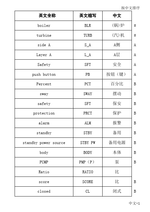
英文全称英文缩写中文boiler BLR(锅)炉#turbine TURB(汽)机#side A S_A A侧ALayer A L_A A层ASafety SFT安全A push button PB按钮(键)A Percent PCT百分比Bsway SWAY摆动Bsafety SFT保安B protection PRCT保护B alarm ALM报警Bstandby STBY备用B standby power source STBY PW备用电源B body BODY本体BPUMP PMP(P)泵BRatio RATIO比score SCORE比Bclosed CL闭式Bclosed circulating water CL CIR WTR闭式循环水B lock LOCK闭锁B lock close LOCK CL闭锁关Block open LOCK OPN闭锁开B wall temperature WALL TEM壁温B transformer XFMR变压器B make-up water MK UP WTR补水Bmake-up oil MK UP OIL补油Bnon symmetry N_SYM不对称B Heating HTG采暖Creference REF参考CStorehouse SH仓Coperation OPR操作C slot SLOT槽CSide SIDE侧C side wall SIDE WALL侧墙C measurement point MSMNT PNT测点C layer LAYER层C differential DIFF差动Cdifferential pressure DIF PRS(DP)差压(压差)C diesel engine DSL柴油机C plant service transformer P_XFMR厂变Cplant service lowerP_L_XFMR厂低变C transformerWorkshop WORKSHOP厂房Cplant service higherP_L_XFMR厂高变C transformerplant inner PLNT INN厂内C Plant PLNT厂用C Plant service power rate PLNT PW RATE厂用电率C Over speed OVER SPD超速C over temperature OVER TEM超温C programmed control PRGC程控C cog COG齿Ccog COG齿部CGear GEAR齿轮CCharge CHARGE充电C extraction steam EXTR抽汽C tap TAP抽头Coutlet OUTL出口COutgoing water OUTG WTR出水C outgoing wire OUTG WIRE出线Cslag remover SLGRMV 出渣机,除渣机CPrecipitator PREC除尘器C Demineralized DEMINE除盐的C Demineralized device DEMINR除盐装置C deaerator DEA除氧器Ctreatment TRMT处理C drum DRUM传动CSensor SSR传感器Csurge SURGE喘震C soot blow SBW吹灰C soot blower SBWR吹灰器C purge PURGE吹扫Cpurity PURITY纯度C classifier CLFR粗粉分离器C open demand OPN DMD打开命令D (front)big platen BIG PLTN大屏D >>大于Ddamper DMPR挡板D conductivity CONDT导电度D steam lead pipe STMLP导汽管D pilot PLT导向D pilot bearing PLT BEAR导向轴承Dguide vane GDVN导叶D Low LOW(LO)低D Low voltage LOW VOLT低电压D low pressure auxiliary LOW AUX低辅D low pressure heater LPH低加D low frequency LOW FREQ低频D low speed LOW SPD低速D low temperature LOW TEM低温D low limit LOW LMT低限D low pressure cylinder LPC低压缸D low pressure LOW PRS低压力D <<低于D Bottom BTM底DStage one STG I第一级DPoint PNT点DIgnition IGNT点火DIgnitor IGNTR点火器D electric magnetic MAG电磁D electric magnetic valve MAG V电磁阀D motor operated MO电动D motor operated regulatingMOV电动调节门D valveMotor drive speedMDSGOP电动调速油泵D governing oil pumpmotor drive feedwater pump MDFP电动给水泵D motor operated valve MOV电动门D electrical work KWH电度Delectric motor MTR电机(电动机)D current CRRT电流DCircuit CCT电路Dvoltage VOLT电压D voltage loop VOLT LOOP电压回路DPower supply PW电源D regulating stage RGL STG调节级Dregulate valve RGL V调节门Dgoverning valve GVN V调速汽门D speed governor SPD GVNR调速器D Governing oil GVN OIL(GO)调速油phase modifier,phasemodulatorPH MDFR调相机D adjusting ADJ调整D butterfly valve BFV蝶阀D top TOP顶D ceiling CLNG顶棚Djacking JACK顶轴D intermittent INTMT定期(排污)Dintermittent blow downflash tank INTMT BLDNFLTK定期排污扩容器DFixed value FV定值D stator STAT定子D motive power MTV动力D moving blade M_BLD动叶片D act ACT动作D coal blocking COAL BLOCK堵煤D blocking BLOCK堵塞D End face END FACE端DShort circuit SC短路D Section#段Dbreaker BRKR断路器D cut off the water supply WTR CUT断水D disconnecting DISCON断线D symmetry SYM对称D atmospheric relief valve ATM REL VLV对空排汽门D collar COLLAR轭部E secondary air SA二次风E secondary air damper SAD二次风挡板E generator transformer unit GXU发变组F generator GEN发电机F valve V阀门Fvalve position POS 阀位/位置反馈Fflange FLAN法兰F tippler TPLR翻车机F feedback FDBK反馈F reverse RVRS反向F reversal rotation RRT反转Fmode MODE方式F orientation ORT方向F Discharge steam DISCH STM放汽F discharge water DISCH WTR放水F Discharge oil DISCH OIL放油F Non NON非F non drive end N_DRV_E非驱动端F isolating platen ISLT PLTN分隔屏F Separator SEP分离器F area AREA分区FBranch BRCH分支Fbin,pulverized coalBIN粉仓F bunkerPC level PC LVL粉位FAir flow AIR FLOW风量FWindbox WINDBOX风箱FAuxiliary AUX辅助F Load LOAD负荷F negative pressure-P负压F Duplicate DUP复FComplex COMP复合F two-velocity stage TVS复速级F Reset RSET复位Fvice VICE副FHigh HIGH(HI)高Ghigh voltage standbyHVSX高备变G transformerhigh voltage HIGH VOLT高电压G high pressure auxiliary HIGH AUX高辅G high pressure header HPH高加G high energy spark ignitor HESI高能点火器G high speed HIGH SPD高速G high level water box HLWB高位水箱G high temperature HIGH TEM高温G high limit HIGH LMT高限G high pressure cylinder HPC高压缸G high pressure HIGH PRS高压力Ghigh intermediate pressureHIPC高中压缸G cylinderisolate ISLT隔离G pulverized coal feeder PVL FDR给粉机G(coal)feeder COAL FDR给煤机G feedwater FEED WTR给水G industrial water IND WTR工业水G working WORK工作G operating transformer OX工作变压器G operating power O_PW工作电源G Common COM公用G common transformer CX公用变G Power PW功率G steam supply STM SPL供汽GH2supply H2SPL供氢Goil supply OIL SPL供油G Fault FAULT故障Gclose CL关G close demand CD关命令G Closed position CP关状态G Pipe PIP管,管道G Pipe wall PIP WALL管壁GContainer CTNR罐Galarm window ALM WIN光字牌G cabinet CAB柜GBoiler BLR锅炉G boiler hall BLR HALL锅炉房G over load OV LOAD过负荷G over excitator OV EXCTR过励磁G over current OV CRRT过流G filter FLTR过滤器G superheated SH过热G superheater SHTR过热器G superheated steam SH STM过热蒸汽G over speed OV SPD过速G over voltage OV VOLT过压G overload OV LOAD过载G oxygen content O2CT含氧量H Number NO.号(量词)H compose CMPS合成H close switch CL SWTH合闸H box BOX盒HBack BA后H rear platen REAR PLTN后屏HSliding stop pushingbearingSSPB滑动止推轴承H Pilot valve PLT V滑阀H ash hopper ASH HOP灰斗Hreturn(oil,water)RTN(OIL,WTR)回(油,水)Hreturn fuel fan RFF回料风机H return air RTN AIR回送风H converge CNVG汇流H scanner SCNR火检H flame FLM火焰H flame intensity FLM INTS火焰强度H Nozzle NOZZLE火嘴H turbine side TURB SIDE机端J Machine room MCH RM机房J Cabinet CAB机柜J mechanical MCHN机械J unit UNIT机组J active ACTIVE激励JStage STG级JLimit LMT极限J steam header STM HDR集汽联箱J water collector WTR CLCT集水箱J header HDR集箱J calculation CAL计算J relay RELAY继电器Jheater HTR加热器J heat steam HEAT STM加热蒸汽Jspeed up SPD UP加速Jcrevice CRVC夹层Jcrevice CRVC间隙Jmonitor MNTR监视JReduce REDR减少Jslow down SLOW DN减速JDesuperheat DSH减温Jtemperature and pressurePRS/TEM REDR减温减压器J reducerDesuperheater DSHR减温器J pressure reducer valve PRS REDR V减压阀Jtest TEST检测J maintenance MAINTENACE检修Jexchanger EXCHR交换器J alternating current AC交流J rubber ball RBBR BALL胶球J corner CRNR角Jground GND接地JThrottle THRL节流J end END结束J throttle THTTL截止JMetal MTL金属JOnly ONLY仅J Emergency EMG紧急Jemergency relieve oilEMG RLV OIL V紧急放油阀J valveIngoing ING进J ingoing line ING LINE进线J fine treatment FINE TRMT精处理J clean CLEAN净J Purity oil chamber PUR OC净油室Jradial/axial RAD/AXI径向J Radial bearing RBEAR径向轴承J stationary blade S_BLD静叶片J Local LCL就地J Isolation ISLT绝缘Jswitch SWTH开关Kstart STR开始Kopen OPN开式K open circulating OPN CIR开式循环K open circulating water OPN CIR WTR开式循环水K opened status OP开状态K flame proof oil FPO抗燃油K shell SHELL壳体K governing GVN可调速的Kair side AIR_S空侧K Air AIR空气K air preheater APH空预器K Control CTL控制KControl demand CTL DMD 控制命令(对调节阀)Kcontrol room CTL ROOM控制室Kcontrol box CTL BOX控制箱Krun back RB快速减负荷Kflash tank FLTK扩容器Kcold air COLD AIR冷风Lcooling CLG冷却L cooling air(blower)fan CLG AIR FAN冷却风机L cooler CLR冷却器L oil cooler OIL CLR冷油器Lcool reheat COOL RHT冷再热L ion ION离子L vertical type VERT立式L Moment MNT力矩excitation EXCT励磁Lexcitator EXCTR励磁机L excitator side EXCTR SIDE励端L continue blowdown CTN BLDN连排Lcontinue blowdownCTN BLDN FLTK连排扩容器L flashtankconnector CNTR连通管Lcombined steam valve CSV联合汽门L interconnection INTRCT联络L interlock INTRLK联锁Lheader HDR联箱L zero sequence0_SEQ零序L flow FLW流量L Ail leak AL漏风Lfurnace FNC炉膛Lfilter FLTR滤网L oil filter OIL FLTR滤油器L rate RATE率Lmotor MTR马达MPulse PULSE脉冲Mmatch MATCH满足M Pulverized coal PUL煤粉M bin BIN煤粉仓M Sealing SEAL密封M seal water SEAL WTR密封水Mseal oil SEAL OIL密封油Mcoal mill MILL磨煤机M worn out WNUT磨损M bowl BOWL磨碗M the last stage L_STG末级M header HDR母管Mbus BUS母线Minner INN 内,内侧,内部Nnatrium NA钠Ninverse INVS逆Ncheck valve,non-returnvalveCHK V逆止门N mesh MESH啮合N condensate CND凝结N condensated water CND WTR凝结水N condensate pump CND P凝结水泵N condenser CNSR凝汽器N torsional oscillation TOROSC扭振N Density DSTY浓度N steam air heater SAH暖风器N coupler CPLR耦合器Orow ROW排(量词)P pulverized coal exhauster PCE排粉机P Exhaust EXH排风PExhauster EXHR排风机P Vent VENT排空P Exhaust steam EXH STM排汽P Exhaust water EXH WTR排水P Blowdown BLDN排污Pflue gas FLUE GAS排烟P exhaust gas fan EGF排烟风机P Exhaust oil EXH OIL排油P turning TURN盘车Ppanel face PNFC盘面P bypass BYPS旁路Pspray SPRAY喷水P expansion EXP膨胀P belt BELT皮带P Eccentricity ECNT偏心度PFrequency FREQ频率Pplaten fan PLTN FAN屏风机P platen superheat P_SHTR屏式过热器P start STR启动Q Start demand STRD启动指令Qpneumatic PNMTC气动Q gas GAS气体QSteam STM汽QDrum DRUM汽包Qturbine-driven feedwaterTDFP汽动给水泵Q pumpsteam-driven oil pump SDOP汽动油泵Qsteam sealing,steam sealGLD汽封Q glandcylinder CYL汽缸Qturbine TURB汽机Q steam temperature STM TEM汽温Q front FR前Q front/back F/B前后Qbooster pump BP前置泵Q force FORCE强制QWall WALL墙QSwitch SWTH切换Q H2side H2_S氢侧Q light LIGHT轻Qwash WASH清洗Qarea AREA区Q drive end DRV_E驱动端Q whole plant WHL PLNT全厂Q whole day WHL DAY全天Q all phases3PH全相Q phase lose PH LOSE缺相Q acknowledge ACK确认Q burning exhaust BRNHT燃尽R Fuel FUEL燃料R Burner BNR燃烧器R winding WND绕组R hot air HOT AIR热风R hot well HOT WELL热井R hot reheat HOT RHT热再热R dissolved DSSLV溶解Rfusible FUSE熔断R fusible cutout FUSE熔断器R inlet INL入口Rlube LUB润滑R lube oil LUB OIL润滑油R tertiary air TA三次风S T valve T V三通阀S up UP上,上部Supper UPP上层S water-supply WTR SPL上水S Set SET设定SExtend EXTD伸进S step up STEP UP升压S Economizer ECON省煤器S failure FAIL失败S lose synchronizer LOSE SYN失步S lose magnet LOSE MAG失磁S be out of order NODR失灵S Cobblestone CS石子Saccident ACCD事故SEmergency EMG事故S test TEST试验S Collection CLCT收集S Manual MANL手动S drain water DRN疏水Sdrain water DRN V疏水阀Sdrain tank DRN TK疏水罐S drain water flashtank DRN FLTK疏水扩容器S pulverized coal conveyor PUL CVR输粉机S coal conveyer COAL CVR输煤机S transport XPRT输送Svertical VERT竖直(方向)的Swater WTR水S Water pump WTR P水泵S water treatment WTR TRMT水处理S Water seal WTR SEAL水封Swater wall WTR WALL水冷壁S water curtain WTR CURTAIN水幕Shorizontal HORZ水平(方向)的S humidity HMDT湿度water level WTR LVL水位S water box WTR BOX水箱S forced draft air FD送风S forced draft fan FDF送风机S Speed SPD速度S fast-closing FAST CL速断S Probe PROBE探针Ttrip TRIP跳闸T (iron)core CORE铁芯T stop command SD停止命令T stop position SP停止状态T Channel CHANL通道TDraft DRAFT通风TSynchronizer SCHN 同步器,同操器Tsynchronous SYNCH同期T bobbin BBIN筒体T putting into PUTIN投Toutlet side OUTL SIDE吐出端T thrust THST推力T thrust bearing THST BEAR推力轴承T retract RETR退回,缩回TUngearing UNGEAR脱扣TDewater DWTR脱水T pad PAD瓦(轴承)Wpad PAD瓦块W buchholtz BCHTZ瓦斯W outer OUT外部W network control room NET CTL ROOM网控楼W displace DISP位移Wposition POS位置W temperature TEM(T)温度W interrogation voltage INT VOLT问询电压W Dirty oil chamber DTY OC污油室W reactive power R_PW无功W atomizing ATM雾化Winlet side INL SIDE吸入端Xsystem SYS系统X cyclone separator CSEP细粉分离器X down DN下Xlower LWR下层,低层X downcomer DNCMR下降管X coil COIL线圈Xlimit LMT限Xphase PH相X relative expansion RLTV EXP相对膨胀X phase angle difference PH DIFF相位差X demagnetizer DEMAG消磁装置X fire_fighting FGHT消防X ridding bubble chamber RBCH消泡箱X disappear DSPPR消失Xboiler feeder water pumpBFPT小汽机X turbine<<小于X Check CHK校正Discharge DISCH泄放X leak LEAK泄漏Xsignal SGNL信号Xstroke STROKE行程X storage battery BATTERY蓄电池X energy storage ENST蓄能器X select,selection SEL选择X circulating CIR循环X circulating water CIR WTR循环水X differential pressure DIFF PRS压差(差压)Y pressure PRS(P)压力Y compressed air CPRESS AIR压缩空气Y gas pass GAS PASS烟道Y gas GAS烟气Y gas temp GAS TEM烟温Ycation CATION阳离子Y O2O2氧Y oxygen content O2CT氧量Y Remote REMO遥控YDemand DMD要求Y hydraulic coupler HD_CPLR液力耦合器Ylevel LVL液位Y Hydraulic pressure HYDP液压Y hydraulic oil HYDL OIL液压油Y primary air PA一次风Y primary air fan PAF一次风机Y primary oil PAO一次油Y 1st extraction1ST EXTR一段抽汽Y Stage one STG I一级Y to indicator TO INDCT仪(器)用Y Closed CD已关,关状态Y abnormal ABNM异常Y overflow OVFL溢Y overflow station OVFL STN溢流站Y induced draft air IDA引风Y induced draft fan IDF引风机Y magneto generator MGNT永励机Y Use USE用(使用)YUser USER用户Y customer valve CV用户阀Yoil OIL油Y oil pump OIL P油泵Y hydraulic servomotor HD_MTR油动机Y Oil value OIL VLU油量Yoil pipe OIL PIPE油路Y oil temperature OIL TEM油温Y Oil box OIL BOX油箱Y oil pressure OIL PRS油压Y oil station OIL STN油站Ypower on PW ON有电Y active power A_PW有功功率Y firing FIRING有火Ywith coal WCL有煤Y right RI右Ypreheat PRHT预热Y preheat pipe PRHT PIP预热管道Y source SRC源Yremote RMT远方Ypermit PMT允许YRun RUN运行Y Running position RUNP运行状态Y turn TURN匝间ZReheat RHT再热Zreheater RHTR再热器Z reheated steam RHT STM再热蒸汽Z regeneration RGEN再生Z recirculate RECIR再循环Z recirculating valve RECIR V再循环阀Z behind BH在…的后面Zdirty DIRTY脏Zincreate INC增加ZDregs DRG渣ZStation STN站Z expansion difference EXP DIFF胀差Z Vacuum VACM真空Z vacuum pump VACM P真空泵Z vacuum break valve VACM BRK V真空破坏阀Z vibration VBRT振动Zsteam chamber STM ROOM蒸汽室Zrectifying RCTF整流的Zrectifier RCTFR整流器Znormal NORM正常Zpositive+正的Zrotation RT正转Z lift LIFT支撑Z lift bearing LIFT BEAR支撑轴承Z branch BRCH支路Z direct current DC直流Z Demand DMD指令,命令Z to TO至Z Middle MID中间,中部ZCenter CTR中心Z Neutral point NTRL PNT中性点Z intermediate pressure INTR PRS中压Zintermediate pressureIPC中压缸Z cylinderheavy HEAVY重Zrenew RENEW重新ZShaft SHFT轴bearing BEAR轴承Z Bearing box BB轴承箱Gland GLD轴封ZBush BUSH轴瓦Z axial displacement AXI DISP轴向位移Z Bearing vibration BEAR VBRT轴振main MAIN主Z main transformer MAIN XFMR主变Z Main electric motor MMTR主电机main turbine MAIN TURB主机Z main steam stop valve MAIN STM V主汽门Z master fuel trip MFT主燃料跳闸Z main steam MAIN STM主蒸汽Zoil tank OIL TK贮油箱Z rotating speed ROT SPD转速Z turning room TURN ROOM转向室Z rotor RTR转子Z equipment EQPMNT装置Zstatus,state ST状态Z automatic AUTO自动Z liberty side LBTY SIDE自由端Z Chief CHF总Z impedance IMPDC阻抗Z Group GP组Combiner COMBNR组件ZMaximum MAX最大Zmaximum continuousMCR最大持续功率Z revolutionMinimum MIN最小Z Pulverized-coal system PCS制粉系统Z Electric ELEC电气DDiaphragm DPHRM隔膜GShockproof SHKPRF耐震N Magnetic control meter MCM磁控表C Reversal washing RWG反冲洗F Left LE左Z。
ASTM_D_4018_99_碳及石墨纤维束的连续长丝抗拉特性的标准试验方法

3.3.14r sf—density of thefiber with sizing3.3.15RC—weight percent of resin(resin content)3.3.16W1—specimen mass4.Summary of Test Methods4.1These test methods include procedures for determining the tensile strength and modulus of a resin-impregnated and consolidated carbonfiber tow.Also included are procedures to measure the mass per unit length and density of the carbon fiber and the resin content of the resin-impregnated and consolidated specimens.4.2MUL—The MUL of thefiber is determined by dividing the mass of a sample of sizedfiber by its length.4.3Density—The density of thefiber is determined using Archimedes’method or a pycnometer method.The recom-mended specimen is desized or unsizedfiber.The ideal immersionfluid is one that completely wets the specimen and provides minimum toxicity or environmental hazard.4.4Resin Content—The resin content(weight percent)of the resin-impregnated and consolidatedfiber is determined by comparing the mass per unit length of the impregnated and consolidated specimen to thefiber mass per unit length.4.5Tensile Properties—The tensile strength and tensile chord modulus of thefiber are determined by the tensile loading to failure of the resin-impregnated and consolidated fiber.The chord modulus is determined between defined strain limits.The purpose of the impregnating resin is to provide the fiber,when consolidated,with sufficient mechanical strength to produce an easily handled test specimen capable of sustaining uniform loading of the individualfilaments in the specimen. The resin shall be compatible with thefiber and any size applied to it.The strain capability of the consolidated resin shall be at least twice the strain capability of thefiber.5.Significance and Use5.1The properties determined by these test methods are of value in material specifications,qualifications,data base gen-eration,certification,research,and development.5.2These test methods are intended for the testing offibers that have been specifically developed for use as reinforcing agents in advanced composite structures.The test results of an impregnated and consolidatedfiber should be representative of the strength and modulus that are available in the material when used as intended.The performance offibers in different resin systems can vary significantly so that correlations be-tween results using these test methods and composite testing may not always be obtained.5.3The reproducibility of test results is dependent upon precise control over all test conditions.Resin type,content and distribution,curing process,filament alignment,gripping in the testing machine,and alignment in the testing machine are of special importance.5.4The measured strengths offibers are not unique quan-tities and test results are strongly dependent on the test methods used.Therefore the test method described here will not necessarily give the same mean strengths or standard devia-tions as those obtained from singlefilaments,dryfibers, composite laminas,or composite laminates.6.Apparatus6.1Three sets of apparatus are required.One set is for resin impregnation of thefiber.A second set is for curing the resin-impregnated specimens.A third set is for tensile testing the resin-impregnated and consolidated specimens.Optional apparatus may be used for applying end tabs to the specimens and removing sizing.6.1.1Resin Impregnation—The goal of the resin-impregnation apparatus is to apply and uniformly impregnate resin into thefiber.This is normally achieved by dipping the fiber into the resin and then working the wetfiber over rolls or through a die,or both.While automated apparatuses are preferred for consistency,any apparatus which achieves uni-form impregnation of35to60%resin by weight and does not damage thefiber is acceptable.6.1.2Consolidation—An apparatus to hold the impregnated specimens under tension during consolidation is required. 6.1.3Optional End Tabs—An apparatus to cast resin end tabs on specimens may be used.Apparatuses to apply and align other forms of end tabs such as bonded on cardboard or metal tabs may also be used.6.1.4Testing—A tensile testing machine and recorder meet-ing the requirements of Practices E4at the maximum expected test load are required.The load recording device shall be coordinated with the extensometer and strain recorder to assure that the corresponding load and elongation of the specimen are recorded at essentially the same time.The testing machine shall also have the following features:6.1.4.1Grips—Grips suitable for loading the tabbed or untabbed specimen without damaging it are required.For resin tabbed specimens a custom grip is generally required.For untabbed or cardboard tabbed specimens pneumatic or hydrau-lically powered grips are typically used.Different grip pressure settings may be required for differentfibers.6.1.4.2Jaws—Jaws compatible with the grips and capable of holding a specimen without damaging it are required.For untabbed specimens,flat jaws with rubber or other compliant materials bonded to the face are generally used.Sandpaper may also be placed on the grips to reduce slippage.For cardboard tabbed specimens serrated jaws are generally used. Jaws should be inspected regularly and cleaned or repaired as required.6.1.4.3Extensometer and Recorder—An extensometer and recording device in accordance with the requirements of Practice E83Class B-2are required.The extensometer and recorder shall be coordinated with the tensile testing machine so that the corresponding load and elongation of the specimen are recorded at essentially the same time.6.1.4.4Balance,Analytical—Accuracy of60.0002g for mass per unit length,density,and resin or size content determinations.6.1.4.5Balance,Laboratory—Accuracy of60.1g for mea-suring components of resin.6.1.4.6Length Measuring Devices—Devices to measure the length of impregnated and consolidated specimens and dry fiber to62-mm accuracy are required.6.1.4.7Density Measuring Device—See Test Methods D70,D3800,or D5550.6.1.4.8Forced Air Oven—A forced air oven of sufficient size and temperature capabilities to cure the impregnatedfiber on the curing device.The temperature shall be controlled to 610°C.7.Reagents and Materials7.1Reagent Water—Unless otherwise indicated,references to water shall be understood to mean reagent water as defined by Type III of Specification D1193.7.2Resin.7.3Commercial Grade Solvent,(optional)for resin dilu-tion.7.4Hardener or Catalyst.7.5Surfactant(optional).8.Test Specimens8.1Mass per Unit Length Specimen—The specimen to measure mass per unit length is a1-m minimum length offiber in the form in which it is intended to be used.Test one specimen per sample.Coil the specimen into a usable form for testing.Care is required to not damage and losefilaments from the specimen.8.2Density Specimen—Density specimens may be sized, unsized,or desized material.Unsized or desized samples are preferred.Test one specimen per sample.A1–m minimum length is required for Test Method D3800.For methods in Test Methods D70and D5550,a suitable volume tofill the container is recommended.Coil the specimen into a usable form for testing.Care is required to not damage and lose filaments from the specimen.8.3Tensile Test Specimen—The tensile specimen shall be a tabbed or untabbed resin-impregnated and consolidatedfiber. Tabbed specimens shall have a150-mm gage length between the tabs.Untabbed specimens shall be of sufficient length to allow a150-mm gage length between the grips when they are tested.Samples with3000filaments or less may be tested using specimens of more than onefiber bundle to facilitate handling. Combine the bundles before resin impregnation and count the test results as one specimen.Test a minimum of four test specimens per sample.Separate test specimens for modulus and strength determination are permitted;however,four speci-mens for each test are required.Specimens that are fuzzy, curved,not uniform in cross section,have brokenfilaments, resin lumps,or other observable defects should be rejected unless they are representative of the material being tested. 9.Conditioning9.1Fibers that adsorb less than0.5%moisture by weight at 2362°C and90%or greater relative humidity require no conditioning before testing.Conduct mass per unit length, density,and tensile testing for these materials at2367°C and 50620%relative humidity unless other conditions are the variables of interest.9.2Conditionfibers that adsorb more than0.5%moisture by weight(at2362°C and90%or greater relative humidity) for a minimum of24h at2362°C and50610%relative humidity.Conduct mass per unit length and density testing at 2362°C and50610%relative humidity unless other conditions are the variables of interest.Conduct tensile testing at2367°C and50620%relative humidity unless other conditions are the variables of interest.9.3To determine moisture adsorption,dry a minimum of five mass per unit-type specimens at12065°C for24h in a circulating air oven.Cool samples in a desiccator.Remove samples from desiccator one at a time and immediately weigh them.Place samples in a humidity chamber and maintain at23 62°C and90%or greater relative humidity for24h.Remove samples from the humidity chamber one at a time and weigh immediately.9.4If all specimens are conditioned for24h and mass per unit length and density testing are performed at2362°C and 50610%relative humidity,then no testing for moisture adsorption is required.9.5Moisture adsorption testing is only required once annu-ally for a standard product.10.Specimen Preparation10.1Mass per Unit Length—No preparation is required. The sample is taken from a package of material as it is intended to be used.10.2Density—The preferred density specimen is a desized or unsizedfiber.This eliminates any need to correct for the density of the sizing.The sizing may be removed using solvent extraction,pyrolysis,or other means.An example method is described in Appendix X1.An unsized sample of a sizedfiber would have to be collected during the production of thefiber and is therefore not recommended.10.3Tensile Test—The tensile test specimen must be im-pregnated with resin and consolidated before testing.10.3.1Resin Preparation—Any resin that meets the re-quirements of4.5may be used.The resin when combined with thefiber shall produce a composite(reinforcement/matrix) failure.A resin generally found satisfactory is a combination of bisphenol A(or bisphenol F)epoxy and diethyltoluene diamine in the weight ratio of3.9:1.A solvent that lowers the viscosity of a resin mixture or softens the sizing,or both,may be selected for use with the resin.The amount and type of solvent used will vary with the product and apparatus used for impregnation.Prepare and store the resin in accordance with the manufacturer’s instructions.10.3.2Fiber Impregnation—The resin shall be maintained within a suitable viscosity or temperature range throughout the impregnation process that assures reproducible specimen con-stituency and quality.An automated impregnation device is recommended but not required.The objective of impregnation is a uniform,well-collimated strand with adequate resin, content,typically35to60%by weight.10.3.2.1Wind or attach the impregnatedfiber to a rack or other device to hold it under tension during consolidation. 10.3.2.2Check the consolidated impregnatedfiber resin content at least daily to ensure adequate resin pickup.Deter-mine the mass of a known length of impregnated and consoli-datedfipute the resin content using the mass per unit length of thefiber as a reference.10.3.2.3Tabbing—End tabs may be applied to the impreg-nated and consolidated specimens but are not required.End tab material must adequately grip the specimen without slipping. Heavy paper or poster board have been used successfullyastabs.The distance between tabs shall be150mm.11.Procedure11.1Mass per Unit Length—Take the mass per unit length specimen from thefiber in the same form as it is intended to be used.Testfiber with size with the size on thefiber.Test one specimen per sample.11.1.1Using a calibrated measuring device measure a minimum of a1-m(62-mm)length offiber.Hold thefiber under light hand tension while measuring and cutting it.Coil thefiber onto a usable form taking care not to damage or lose filaments.11.1.2Determine the mass of the specimen using an ana-lytical balance.11.1.3Retests—Reject any specimen which has an obvious flaw or deviation from the requirements of these test methods. Prepare a new or spare specimen from the same sample and test to replace any specimens eliminated in accordance with this paragraph.11.1.3.1Discard test results for any condition that compro-mises the integrity of the test.These conditions must be documented.11.1.3.2Retest any suspect single specimen or sample. Retesting of specimens requires twice the number of specimens that were suspect.Retesting of a sample requires twice the number of specimens that were tested in the suspect sample. The average result of the retested specimens shall replace the original value.However,all values must be recorded.11.2Density—Test density in accordance with Method A of Test Methods D3800(for Archimedes’method)or D70/ D5550(for a pycnometer method)with modifications.The preferred density sample is unsized or desizedfiber.Test one specimen per sample.Coil thefiber into a suitable form taking care not to damage or losefilaments.11.2.1Retests—Any specimen that has an obviousflaw or deviation from the requirements of these test methods shall be rejected.Prepare a new or spare specimen from the same sample and test to replace any specimens eliminated in accordance with this paragraph.11.2.1.1Discard test results for any condition that compro-mises the integrity of the test.These conditions must be documented.11.2.1.2Retest any suspect single specimen or sample. Retesting of specimens requires twice the number of specimens that were suspect.Retesting of a sample requires twice the number of specimens that were tested in the suspect sample. The average result of the retested specimens shall replace the original value.However,all values must be recorded.11.3Tensile Test—Test the impregnated and consolidated fiber in a calibrated tensile testing machine using a calibrated extensometer.Test a minimum of four specimens for strength and modulus.These may be the same four specimens or two sets of four specimens.(If the extensometer causes premature tensile failure it may be necessary to test four additional specimens without the extensometer for strength only.)11.3.1Install the appropriate grips and jaws into the tensile testing machine.For untabbed specimens set the distance between the grips to150mm.11.3.2Set the speed of the testing machine.The maximum acceptable speed is250mm/min(10in./min).The maximum practical speed may be limited by the speed of data sampling or recording equipment.11.3.3Select the appropriate load range of the tensile testing machine.11.3.4Set the speed of any recording or sampling equip-ment as required.11.3.5Place the specimen in the jaws and carefully align it so that it is centered in the jaws and aligned with the loading axis.Close the grips assuring that the specimen remains aligned.11.3.6Preload the specimen to the appropriate load in accordance with Table1.Determine the load using the ex-pected modulus and cross-sectional area of thefiber.11.3.7Attach the extensometer if modulus is to be mea-sured.Take particular care not to damage or cutfilaments. 11.3.8Start the recording or sampling equipment and the tensile testing machine.11.3.9When the maximum strain required for modulus calculation has been exceeded,the extensometer may be removed.This may be done while the test is in progress or after stopping the testing machine.Take particular care not to damage or cutfilaments.11.3.10Test the specimen to failure.Observe the failure of specimen.11.3.11Record the failure load and the load at the strains in accordance with Table2for use in calculating the chord modulus.11.3.12Retests—Any specimen that has an obviousflaw or deviation from the requirements of these test methods shall be rejected.Prepare a new or spare specimen from the same sample and test to replace any specimens eliminated in accordance with this paragraph.11.3.12.1Discard test results for any condition that com-promises the integrity of the test.These conditions must be documented.Examples of these conditions include slippage of the specimen or extensometer,breaks in the tabs or grips, breaks at the extensometer attachment points,and abnormal breaks which may be due to poor resin impregnation(see11.4).11.3.12.2Retest any suspect single specimen or sample. Retesting of specimens requires twice the number of specimens that were suspect.Retesting of a sample requires twice the number of specimens that were tested in the suspect sample. The average result of the retested specimens shall replace the original value.However,all values must be recorded.11.4Failure Mode—Record atypical mode and location of failure of individual specimens.Typical failure mode and location may be grouped for thefiber.Choose,if possible,a standard description using the three-part failure mode code that is shown in Fig.111.5Grip/Tab Failures—Reexamine the means of load introduction into the material if a significant fraction of failuresTABLE1Maximum PreloadsTypical Product Maximum Preload Strain at failure(microstrain)(microstrain)e$120002006000#e<12000100e<6000100in a sample population occur within one specimen width of thetab or grip.Factors considered should include the tab align-ment,tab material,tab adhesive,grip type,grip pressure,andgrip alignment.12.Calculations12.1Mass per Unit Length,MUL —Calculate the mass perunit length of the fiber using the following equation.MUL 5W 1/L (1)where:MUL 5mass per unit length,g/m;W 15mass of the specimen,g;andL 5length of the specimen,m.12.2Density —Calculate the density of the fiber using fol-lowing sets of equations.12.2.1Desized or Unsized Fiber (Preferred)—Use equa-tions found in Test Methods D 3800,D 70,or D 5550.12.2.2Sized Fiber —Determine the fiber density as follows:r f 5r sf –k c (2)where:r f 5fiber density,g/cm 3;r sf 5density of fiber +sizing,g;and k c 5correction factor (if required).(k c is determined by means of repeated tests on sized and desized or unsized samples to correlate sized fiber results with the preferred technique.k c may be a function of size level and size type.A correction factor is not required if the test differences are less than 1.0%of the preferred technique result.)12.3Tensile Test :12.3.1Resin Content —Calculate the resin content of the impregnated and consolidated fiber using the following equa-tion:RC 5100~12~MUL /MUL i !!(3)where:RC 5resin content,weight %;MUL 5mass per unit length of fiber,g/m;and MUL i 5mass per unit length of the impregnated and consolidated fiber,g/m.12.3.2Tensile Strength —Calculate the tensile strength of the fiber using the following equation:Tensile Strength ~MPa !5A 3P 3r f /MUL (4)where:P 5maximum load measured in tensile test,N (lb);r f 5fiber density,g/cm 3;MUL 5fiber mass per unit length,g/m;and A 5unit conversion factor (1if load in N).12.3.3Tensile Modulus —Calculate the tensile chord modu-lus of the fiber between the strain values in accordance with 11.3.11using the following equation:E 5B 3~P u 2P l !3r f /~~e u 2e l !3MUL !(5)where:E 5fiber chord modulus,GPa;P u 5tensile load at upper strain limit,N (lb);P l 5tensile load at lower strain limit,N (lb);r f 5fiber density,g/cm 3;e u 5upper strain limit,microstrain;e l 5lower strain limit,microstrain;MUL 5fiber mass unit length,g/m;and B 5unit conversion factor (10−3if load is in N).13.Report 13.1Report the following information:13.1.1MUL Report :13.1.1.1Complete identification of the samples tested to assure traceability of test results,13.1.1.2Date of test,13.1.1.3Test facility,13.1.1.4Identification of the individual performing test,13.1.1.5MUL of the specimens tested,and 13.1.1.6Any deviations from these test methods.13.1.2Density Report :13.1.2.1Complete identification of the samples tested to assure traceability of test results,13.1.2.2Date of test,13.1.2.3Test facility,13.1.2.4Identification of the individual performing test,TABLE 2Chord Modulus Strain LimitsTypical Product Chord ModulusStrain at failure (microstrain)strains (microstrain)lower uppere $12000100060006000#e <1200010003000e <60005001500FIG.1Three-Part Failure ModeCode13.1.2.5Immersionfluid and degassing technique if appro-priate,13.1.2.6Density of the specimens tested,and13.1.2.7Any deviations from these test methods.13.1.3Tensile Test Report:13.1.3.1Complete identification of the samples tested to assure traceability of test results,13.1.3.2Date of test,13.1.3.3Test facility,13.1.3.4Identification of the individual performing test, 13.1.3.5Impregnation apparatus,resin,and consolidation or cure cycle used,13.1.3.6Tensile testing apparatus,13.1.3.7Individual and average tensile strength and tensile chord modulus of the specimens tested,and13.1.3.8Reason for specimen rejection and atypical speci-men failure modes,as well as a typical failure mode.13.1.3.9Any deviations from these test methods.14.Precision and Bias14.1Precision—The precision of the procedures for mea-suring MUL,density,tensile strength and tensile chord modu-lus,and weight percent size is being determined.14.2Bias—Since there is no accepted reference material suitable for the procedure for measuring tensile strength and tensile chord modulus,bias has not been determined.The procedures for measuring MUL and weight percent size have no bias because the values of MUL and weight percent size are defined only in terms of these test methods.APPENDIX(Nonmandatory Information)X1.REMOVING THE SIZE FROM SIZED FIBER SPECIMENS AND DETERMINING THE PERCENT SIZING CONTENTX1.1ScopeX1.1.1This test method describes a procedure for removing the size from sizedfiber specimens and determining the percent sizing content.X1.2Summary of Test MethodX1.2.1Sizing is completely pyrolyzed from thefiber by heating the specimen in a furnace under inert atmosphere.A typical temperature and time to accomplish this are450°C for 15min.However,a particular set of time and temperature requirements must be determined for each size andfiber under consideration.X1.3Significance and UseX1.3.1The result of this test method,a desizedfiber specimen,is the preferred specimen for density measurement. X1.3.2This test method may be used to determine the weight percent sizing of thefiber specimen.X1.4ApparatusX1.4.1Electric Furnace—An electric furnace with ad-equate exhaust ventilation and capable of the temperature required to pyrolyze the sizing under consideration.The furnace is supplied with nitrogen to maintain an inert atmo-sphere.X1.4.2Flow Meter—Aflow meter for nitrogen gas with a recommended range from0to50L/min for use in the furnace apparatus.X1.4.3Flow Meter—Aflow meter for nitrogen gas with a recommended range from0to10L/min for use in the cool-down sagger apparatus.X1.4.4Desiccator—A desiccator of sufficient size to hold the specimens.X1.4.5Specimen Tray—A specimen tray to hold the speci-mens during pyrolysis and cool down.A stainless steel tray with permanently marked or numbered bins is recommended.X1.4.6Cool-Down Sagger—A cool-down sagger of suffi-cient size to enclose the specimen tray.Stainless steel construc-tion is recommended to avoid heat damage from the hot specimen tray.The cool-down sagger is supplied with nitrogen to maintain an inert atmosphere.X1.5Test SpecimenX1.5.1Test one test specimen per sample.X1.6ConditioningX1.6.1See Section9.X1.7ProcedureX1.7.1Cut a minimum1-m specimen offiber.Coil thefiber into a usable form taking care not to damage or losefilaments. It is recommended that the specimen mass not exceed2g.X1.7.2Determine the mass of the specimen using an analytical balance with60.0002-g accuracy.X1.7.3Increase the nitrogenflow in the preheated furnace to reduce the influx of air.Remove a preheated tray from the furnace and place the specimens in the tray.X1.7.4Return the tray to the preheated furnace for the required time at temperature.Maintain the furnace nitrogen flow at a sufficient rate to maintain an inert atmosphere but not so high as to remove loosefilaments from the samples.X1.7.5After the pyrolysis is complete,remove the speci-men tray from the furnace and place in the cool-down sagger under nitrogen purge for approximately15min.Maintain the sagger nitrogenflow at a sufficient rate to maintain an inert atmosphere but not so high as to remove loosefilaments from the samples.X1.7.6At the end of the cool-down period,remove the tray from the sagger and determine the mass of the desizedfiber immediately.If this weighing will be delayed,place the specimens in a desiccator to prevent moisture adsorption on thefiber.N OTE X1.1—It is necessary to place the desized fiber in a desiccator forthis procedure for two reasons.First,the mass differences between thesized and desized fiber are small because of the small mass of size appliedto the fiber (typically 1%).Second,the desized fiber has a higher wateradsorption than the sized or unsized fiber as a result of a small amount ofoxidation occurring during this test.It is not necessary to keep thespecimen desiccated for subsequent use as a density specimen because thedensity test has a 50to 60%mass difference making it much less sensitiveto moisture adsorption affects.X1.7.7Run a standard of unsized fiber periodically to assurethat no significant fiber weight loss is occurring.X1.7.8Perform a test pyrolysis condition study with anynew sizing or fiber to determine the conditions under which thesize is pyrolyzed and the fiber is not affected.Correlate theresults of this study with pyrolysis results from unsized andsized standards or with acid digestion or solvent extractionresults on unsized and sized fiber.Correlation constants deter-mined from this study may be applied to compensate for anydifferences.X1.7.9Retests —Reject any specimen that has an obviousflaw or deviation from the requirements of this test method.Prepare and test a new or spare specimen from the same sampleto replace any specimens eliminated in accordance with thisparagraph.X1.7.9.1Discard test results for any condition which com-promises the integrity of the test.These conditions must bedocumented.X1.7.9.2Any suspect single specimen or sample may be retested using double the number of specimens from the same sample unit.The average result of the retested specimens shall replace the original value.However,all values must be recorded.X1.8Calculations X1.8.1Calculate the percent size content as follows:%size content 5100~W 12W 2!/W 1(X1.1)where:W 15mass of specimen before pyrolysis,g and W 25mass of specimen after pyrolysis,g.X1.8.2Corrections to calculations may be used by applica-tion of correlation constants determined in X1.7.8.X1.9Percent Size Report X1.9.1Report the following information:X1.9.1.1Complete identification of the samples tested to assure traceability of test results,X1.9.1.2Date of test,X1.9.1.3Test facility,X1.9.1.4Pyrolysis conditions,X1.9.1.5Identification of the individual performing test,X1.9.1.6Size of the specimens tested,%,and X1.9.1.7Any deviations from this test method.The American Society for Testing and Materials takes no position respecting the validity of any patent rights asserted in connection with any item mentioned in this ers of this standard are expressly advised that determination of the validity of any such patent rights,and the risk of infringement of such rights,are entirely their own responsibility.This standard is subject to revision at any time by the responsible technical committee and must be reviewed every five years and if not revised,either reapproved or withdrawn.Your comments are invited either for revision of this standard or for additional standards and should be addressed to ASTM Headquarters.Your comments will receive careful consideration at a meeting of the responsible technical committee,which you may attend.If you feel that your comments have not received a fair hearing you should make your views known to the ASTM Committee on Standards,at the address shown below.This standard is copyrighted by ASTM,100Barr Harbor Drive,PO Box C700,West Conshohocken,PA 19428-2959,United States.Individual reprints (single or multiple copies)of this standard may be obtained by contacting ASTM at the above address or at 610-832-9585(phone),610-832-9555(fax),or service@ (e-mail);or through the ASTM website().。
On the Shockley-Read-Hall Model Generation-Recombination in Semiconductors
On the Shockley-Read-Hall Model:Generation-Recombination in SemiconductorsThierry Goudon1,Vera Miljanovi´c2,Christian Schmeiser3January17,2006AbstractThe Shockley-Read-Hall model for generation-recombination of electron-hole pairs insemiconductors based on a quasistationary approximation for electrons in a trappedstate is generalized to distributed trapped states in the forbidden band and to ki-netic transport models for electrons and holes.The quasistationary limit is rigorouslyjustified both for the drift-diffusion and for the kinetic model.Keywords:semiconductor,generation,recombination,drift-diffusion,kinetic modelAMS subject classification:Acknowledgment:This work has been supported by the European IHP network“HYKE-Hyperbolic and Kinetic Equations:Asymptotics,Numerics,Analysis”,contract no.HPRN-CT-2002-00282,and by the Austrian Science Fund,project no.W008(Wissenschaftskolleg ”Differential Equations”).Part of it has been carried out while the second and third authors enjoyed the hospitality of the Universit´e des Sciences et Technologies Lille1.1Team SIMPAF–INRIA Futurs&Labo.Paul Painlev´e UMR8524,CNRS–Universit´e des Sciences et Technologies Lille1,Cit´e Scientifique,F-59655Villeneuve d’Ascq cedex,France.2Wolfgang Pauli Institut,Universit¨a t Wien,Nordbergstraße15C,1090Wien,Austria.3Fakult¨a t f¨u r Mathematik,Universit¨a t Wien,Nordbergstraße15C,1090Wien,Austria&RICAM Linz,¨Osterreichische Akademie der Wissenschaften,Altenbergstr.56,4040Linz,Austria.11IntroductionThe Shockley-Read-Hall (SRH-)model was introduced in 1952[13],[9]to describe the sta-tistics of recombination and generation of holes and electrons in semiconductors occurring through the mechanism of trapping.The transfer of electrons from the valence band to the conduction band is referred to as the generation of electron-hole pairs (or pair-generation process),since not only a free electron is created in the conduction band,but also a hole in the valence band which can contribute to the charge current.The inverse process is termed recombination of electron-hole pairs.The bandgap between the upper edge of the valence band and the lower edge of the conduction band is very large in semiconductors,which means that a big amount of energy is needed for a direct band-to-band generation event.The presence of trap levels within the forbidden band caused by crystal impurities facilitates this process,since the jump can be split into two parts,each of them ’cheaper’in terms of energy.The basic mechanisms are illustrated in Figure 1:(a)hole emission (an electron jumps from the valence band to the trapped level),(b)hole capture (an electron moves from an occupied trap to the valence band,a hole disappears),(c)electron emission (an electron jumps from trapped level to the conduction band),(d)electron capture (an electron moves from the conduction band to an unoccupiedtrap).a b cd conduction band trapped level valence bandE v E ce n e r g y of a n e l e c t r o n ,E E Figure 1:The four basic processes of electron-hole recombination.Models for this process involve equations for the densities of electrons in the conduction band,holes in the valence band,and trapped electrons.Basic for the SRH model are the drift-diffusion assumption for the transport of electrons and holes,the assumption of one trap level in the forbidden band,and the assumption that the dynamics of the trapped electrons is quasistationary,which can be motivated by the smallness of the density of trapped states compared to typical carrier densities.This last assumption leads to the elimination of the density of trapped electrons from the system and to a nonlinear effective recombination-generation rate,reminiscent of Michaelis-Menten kinetics in chemistry.This model is an2important ingredient of simulation models for semiconductor devices(see,e.g.,[10],[12]).In this work,two generalizations of the classical SRH model are considered:Instead of a single trapped state,a distribution of trapped states across the forbidden band is allowed and,in a second step,a semiclassical kinetic model including the fermion nature of the charge carriers is introduced.Although direct band-to-band recombination-generation(see, e.g.,[11])and impact ionization(e.g.,[2],[3])have been modelled on the kinetic level before, this is(to the knowledge of the authors)thefirst attempt to derive a’kinetic SRH model’. (We mention also the modelling discussions and numerical simulations in??.) For both the drift-diffusion and the kinetic models with self consistent electricfields ex-istence results and rigorous results concerning the quasistationary limit are proven.For the drift-diffusion problem,the essential estimate is derived similarly to[6],where the quasi-neutral limit has been carried out.For the kinetic model Degond’s approach[4]for the existence of solutions of the Vlasov-Poisson problem is extended.Actually,the existence theory already provides the uniform estimates necessary for passing to the quasistationary limit.In the following section,the drift-diffusion based model is formulated and nondimension-alized,and the SRH-model is formally derived.Section3contains the rigorous justification of the passage to the quasistationary limit.Section4corresponds to Section2,dealing with the kinetic model,and in Section5existence of global solutions for the kinetic model is proven and the quasistationary limit is justified.2The drift-diffusion Shockley-Read-Hall modelWe consider a semiconductor crystal with a forbidden band represented by the energy interval (E v,E c)with the valence band edge E v and the conduction band edge E c.The constant(in space)number density of trap states N tr is obtained by summing up contributions across the forbidden band:N tr= E c E v M tr(E)dE.Here M tr(E)is the energy dependent density of available trapped states.The position density of occupied traps is given byn tr(f tr)(x,t)= E c E v M tr(E)f tr(x,E,t)dE,where f tr(x,E,t)is the fraction of occupied trapped states at position x∈Ω,energy E∈(E v,E c),and time t≥0.Note that0≤f tr≤1should hold from a physical point of view.The evolution of f tr is coupled to those of the density of electrons in the conduction band, denoted by n(x,t)≥0,and the density of holes in the valence band,denoted by p(x,t)≥0. Electrons and holes are oppositely charged.The coupling is expressed through the following3quantitiesS n=1τn N tr n0f tr−n(1−f tr) ,S p=1τp N tr p0(1−f tr)−pf tr ,(1)R n= E c E v S n M tr dE,R p= E c E v S p M tr dE.(2) Indeed,the governing equations are given by∂t f tr=S p−S n=p0τp N tr+nτn N tr−f tr p0+pτp N tr+n0+nτn N tr ,(3)∂t n=∇·J n+R n,J n=µn(U T∇n−n∇V),(4)∂t p=−∇·J p+R p,J p=−µp(U T∇p+p∇V),(5)εs∆V=q(n+n tr(f tr)−p−C).(6) For the current densities J n,J p we use the simplest possible model,the drift diffusion ansatz,with constant mobilitiesµn,µp,and with thermal voltage U T.Moreover,since the trapped states havefixed positions,noflux appears in(3).By R n and R p we denote the recombination-generation rates for n and p,respectively. The rate constants areτn(E),τp(E),n0(E),p0(E),where n0(E)p0(E)=n i2with the energy independent intrinsic density n i.Integration of(3)yields∂t n tr=R p−R n.(7) By adding equations(4),(5),(7),we obtain the continuity equation∂t(p−n−n tr)+∇·(J n+J p)=0,(8) with the total charge density p−n−n tr and the total current density J n+J p.In the Poisson equation(6),V(x,t)is the electrostatic potential,εs the permittivity of the semiconductor material,q the elementary charge,and C=C(x)the given doping profile.Note that ifτn,τp,n0,p0are independent from E,or if there exists only one trap level E trwith M tr(E)=N trδ(E−E tr),then R n=1τn [n0n trN tr−n(1−n tr N tr)],R p=1τp[p0(1−n tr N tr)−p n tr N tr],and the equations(4),(5)together with(7)are a closed system governing the evolution of n,p,and n tr.We now introduce a scaling of n,p,and f tr in order to render the equations(4)-(6) dimensionless:Scaling of parameters:i.M tr→N tr E c−E v M tr.ii.τn,p→¯ττn,p,where¯τis a typical value forτn andτp.iii.µn,p→¯µµn,p,where¯µis a typical value forµn,p.4iv.(n 0,p 0,n i ,C )→¯C(n 0,p 0,n i ,C ),where ¯C is a typical value of C .Scaling of unknowns:v.(n,p )→¯C(n,p ).vi.n tr →N tr n tr .vii.V →U T V .viii.f tr →f tr .Scaling of independent variables:ix.E →E v +(E c −E v )E .x.x →√¯µU T ¯τx ,where the reference length is a typical diffusion length before recombina-tion.xi.t →¯τt ,where the reference time is a typical carrier life time.Dimensionless parameters:xii.λ= εs q ¯C ¯µ¯τ=1¯x εs U T q ¯C is the scaled Debye length.xiii.ε=N tr ¯C is the ratio of the density of traps to the typical doping density,and will be assumed to be small:ε≪1.The scaled system reads:ε∂t f tr =S p (p,f tr )−S n (n,f tr ),S p =1τpp 0(1−f tr )−pf tr ,S n =1τn n 0f tr −n (1−f tr ) ,(9)∂t n =∇·J n +R n (n,f tr ),J n =µn (∇n −n ∇V ),R n = 10S n M tr dE ,(10)∂t p =−∇·J p +R p (p,f tr ),J p =−µp (∇p +p ∇V ),R p = 10S p M tr dE ,(11)λ2∆V =n +εn tr −p −C ,n tr (f tr )= 10f tr M tr dE ,(12)with n 0(E )p 0(E )=n 2i and 10M tr dE =1.5By lettingε→0in(9)formally,we obtain f tr=τn p0+τp nτn(p+p0)+τp(n+n0),and the reduced systemhas the following form∂t n=∇·J n+R(n,p),(13)∂t p=−∇·J p+R(n,p),(14)R(n,p)=(n i2−np) 10M tr(E)τn(E)(p+p0(E))+τp(E)(n+n0(E))dE,(15)λ2∆V=n−p−C.(16) Note that ifτn,τp,n0,p0are independent from E or if there exists only one trap level,thenwe would have the standard Shockley-Read-Hall model,with R=n i2−npτn(p+p0)+τp(n+n0).Existenceand uniqueness of solutions of the limiting system(13)–(16)under the assumptions(21)–(25) stated below is a standard result in semiconductor modelling.A proof can be found in,e.g., [10].3Rigorous derivation of the drift-diffusion Shockley-Read-Hall modelWe consider the system(9)–(12)with the position x varying in a bounded domainΩ∈R3 (all our results are easily extended to the one-and two-dimensional situations),the energy E∈(0,1),and time t>0,subject to initial conditionsn(x,0)=n I(x),p(x,0)=p I(x),f tr(x,E,0)=f tr,I(x,E)(17) and mixed Dirichlet-Neumann boundary conditionsn(x,t)=n D(x,t),p(x,t)=p D(x,t),V(x,t)=V D(x,t)x∈∂ΩD⊂∂Ω(18) and∂n ∂ν(x,t)=∂p∂ν(x,t)=∂V∂ν(x,t)=0x∈∂ΩN:=∂Ω\∂ΩD,(19)whereνis the unit outward normal vector along∂ΩN.We permit the special cases thateither∂ΩD or∂ΩN are empty.More precisely,we assume that either∂ΩD has positive(d−1)-dimensional measure,or it is empty.In the second situation(∂ΩD empty)we haveto assume total charge neutrality,i.e.,Ω(n+εn tr−p−C)dx=0,if∂Ω=∂ΩN.(20)The potential is then only determined up to a(physically irrelevant)additive constant.The following assumptions on the data will be used:For the boundary datan D,p D∈W1,∞loc(Ω×R+t),V D∈L∞loc(R+t,W1,6(Ω)),(21)6for the initial datan I ,p I ∈H 1(Ω)∩L ∞(Ω),0≤f tr,I ≤1,(22) Ω(n I +εn tr (f tr,I )−p I −C )dx =0,if ∂Ω=∂ΩN ,(23)for the doping profile C ∈L ∞(Ω),(24)for the recombination-generation rate constants n 0,p 0,τn ,τp ∈L ∞((0,1)),τn ,τp ≥τmin >0.(25)With these assumptions,a local existence and uniqueness result for the problem (9)–(12),(17)–(19)for fixed positive εcan be proven by a straightforward extension of the approach in[5](see also [10]).In the following,local existence will be assumed,and we shall concentrate on obtaining bounds which guarantee global existence and which are uniform in εas ε→0.For the sake of simplicity,we consider that the data in (21),(22)and (24)do not depend on ε;of course,our strategy works dealing with sequences of data bounded in the mentioned spaces.The following result is a generalization of [6,Lemma 3.1],where the case of homogeneous Neumann boundary conditions and vanishing recombination was treated.Our proof uses a similar approach.Lemma 3.1.Let the assumptions (21)–(25)be satisfied.Then,the solution of (9)–(12),(17)–(19)exists for all times and satisfies n,p ∈L ∞loc ((0,∞),L ∞(Ω))∩L 2loc ((0,∞),H 1(Ω)))uniformly in εas ε→0as well as 0≤f tr ≤1.Proof.Global existence will be a consequence of the following estimates.Introducing the new variables n =n −n D , p =p −p D , C=C −εn tr −n D +p D the equations (10)–(12)take the following form:∂t n =∇·J n +R n −∂t n D ,J n =µn ∇ n +∇n D −( n +n D )∇V ,(26)∂t p =−∇J p +R p −∂t p D ,J p =−µp ∇ p +∇p D +( p +p D )∇V ,(27)λ2∆V = n − p − C.(28)As a consequence of 0≤f tr ≤1, C∈L ∞((0,∞)×Ω)holds.For q ≥2and even,we multiply (26)by n q −1/µn ,(27)by p q −1/µp ,and add:d dt Ω n q qµn + p q qµp dx =−(q −1) Ω n q −2∇ n ∇n dx −(q −1) Ω p q −2∇ p ∇p dx +(q −1) Ω n q −2n ∇ n − p q −2p ∇ p ∇V dx + Ω n q −1µn (R n −∂t n D )+ Ω p q −1µp (R p −∂t p D )=:I 1+I 2+I 3+I 4+I 5.(29)7Using the assumptions on n D ,p D and |R n |≤C (n +1),|R p |≤C (p +1),we estimate I 4≤C Ω| n |q −1(n +1)dx ≤C Ω n q dx +1 ,I 5≤C Ωp q dx +1 .The term I 3can be rewritten as follows:I 3= Ω n q −1∇ n − p q −1∇ p ]∇V dx + Ω n q −2∇ n (n D ∇V )dx − Ω p q −2∇ p (p D ∇V )dx =−1λ2q Ω[ n q − p q ]( n − p − C )dx −1λ2(q −1) Ω n q −1(∇n D ∇V +n D ( n − p − C ) dx +1λ2(q −1) Ωp q −1(∇p D ∇V +p D ( n − p − C ) dx.The second equality uses integration by parts and (28).The first term on the right hand side is the only term of degree q +1.It reflects the quadratic nonlinearity of the problem.Fortunately,it can be written as the sum of a term of degree q and a nonnegative term.By estimation of the terms of degree q using the assumptions on n D and p D as well as ∇V L q (Ω)≤C ( n L q (Ω)+ p L q (Ω)+ CL q (Ω)),we obtain I 3≤−1λ2q Ω[ n q − p q ]( n − p )dx +C Ω( n q + p q )dx +1 ≤C Ω( n q + p q )dx +1 .The integral I 1can be written as I 1=− Ω n q −2|∇n |2dx + Ω n q −2∇n D ∇n dx.(30)By rewriting the integrand in the second integral asn q −2∇n D ∇n = n q −22∇n n q −22∇n Dand applying the Cauchy-Schwarz inequality,we have the following estimate for (30):I 1≤− Ωn q −2|∇n |2dx +Ω n q −2|∇n |2dx Ω n q −2|∇n D |2dx ≤−12 Ω n q −2|∇n |2dx +C n q −2L q ≤−12 Ωn q −2|∇n |2dx +C Ω n q dx +1 .8For I2,the same reasoning(with n and n D replaced by p and p D,respectively)yields an analogous estimate.Collecting our results,we obtaind dt Ω n q qµn+ p q qµp dx≤−12 Ω n q−2|∇n|2dx−12 Ω p q−2|∇p|2dx+C Ω( n q+ p q)dx+1 .(31)Since q≥2is even,thefirst two terms on the right hand side are nonpositive and the Gronwall lemma givesΩ( n q+ p q)dx≤e qCt Ω( n(t=0)q+ p(t=0)q)dx+1 .A uniform-in-q-and-εestimate for n L q, p L q follows,and the uniform-in-εbound in L∞loc((0,∞),L∞(Ω))is obtained in the limit q→∞.The estimate in L2loc((0,∞),H1(Ω)) is then derived by returning to(31)with q=2.Now we are ready for proving the main result of this section.Theorem3.2.Let the assumptions of Theorem3.1be satisfied.Then,asε→0,for every T>0,the solution(f tr,n,p,V)of(9)–(12),(17)–(19)converges with convergence of f tr in L∞((0,T)×Ω×(0,1))weak*,n and p in L2((0,T)×Ω),and V in L2((0,T),H1(Ω)).The limits of n,p,and V satisfy(13)–(19).Proof.The L∞-bounds for f tr,n,and p,and the Poisson equation(12)imply∇V∈L2((0,T)×Ω).From the definition of J n,J p(see(4),(5)),it then follows that J n,J p∈L2((0,T)×Ω).Then(10)and(11)together with R n,R p∈L∞((0,T)×Ω)imply∂t n,∂t p∈L2((0,T),H−1(Ω)).The previous result and the Aubin lemma(see,e.g.,Simon[14,Corollary 4,p.85])gives compactness of n and p in L2((0,T)×Ω).We already know from the Poisson equation that∇V∈L∞((0,T),H1(Ω)).By taking the time derivative of(12),one obtains∂t∆V=∇·(J n+J p),with the consequence that∂t∇V is bounded in L2((0,T)×Ω).Therefore,the Aubin lemma can again be applied as above to prove compactness of∇V in L2((0,T)×Ω).These results and the weak compactness of f tr are sufficient for passing to the limit in the nonlinear terms n∇V,p∇V,nf tr,and pf tr.Let us also remark that∂t n and∂t p are bounded in L2(0,T;H−1(Ω)),so that n,p are compact in C0([0,T];L2(Ω)−weak).With this remark the initial data for the limit equation makes sense.By the uniqueness result for the limiting problem(mentioned at the end of Section2),the convergence is not restricted to subsequences.94A kinetic Shockley-Read-Hall modelIn this section we replace the drift-diffusion model for electrons and holes by a semiclassical kinetic transport model.It is governed by the system∂t f n+v n(k)·∇x f n+q∇x V·∇k f n=Q n(f n)+Q n,r(f n,f tr),(32)∂t f p+v p(k)·∇x f p−q ∇x V·∇k f p=Q p(f p)+Q p,r(f p,f tr),(33)∂t f tr=S p(f p,f tr)−S n(f n,f tr),(34)εs∆x V=q(n+n tr−p−C),(35) where f i(x,k,t)represents the particle distribution function(with i=n for electrons and i=p for holes)at time t≥0,at the position x∈R3,and at the wave vector(or generalized momentum)k∈R3.All functions of k have the periodicity of the reciprocal lattice of the semiconductor crystal.Equivalently,we shall consider only k∈B,where B is the Brillouin zone,i.e.,the set of all k which are closer to the origin than to any other lattice point,with periodic boundary conditions on∂B.The coefficient functions v n(k)and v p(k)denote the electron and hole velocities,respec-tively,which are related to the electron and hole band diagrams byv n(k)=∇kεn(k)/ ,v p(k)=−∇kεp(k)/ ,where is the reduced Planck constant.The elementary charge is still denoted by q.The collision operators Q n and Q p describe the interactions between the particles and the crystal lattice.They involve several physical phenomena and can be written in the general formQ n(f n)= B Φn(k,k′)[M n f′n(1−f n)−M′n f n(1−f′n)]dk′,(36)Q p(f p)= B Φp(k,k′)[M p f′p(1−f p)−M′p f p(1−f′p)]dk′,(37) with the primes denoting evaluation at k′,with the nonnegative,symmetric scattering cross sections Φn(k,k′)and Φp(k,k′),and with the MaxwelliansM n(k)=c n exp(−εn(k)/k B T),M p(k)=c p exp(−εp(k)/k B T),where k B T is the thermal energy of the semiconductor crystal lattice and the constants c n, c p are chosen such that B M n dk= B M p dk=1.The remaining collision operators Q n,r(f n,f tr)and Q p,r(f p,f tr)model the generation and recombination processes and are given byQ n,r(f n,f tr)= E c E vˆS n(f n,f tr)M tr dE,(38)10withˆS n (f n ,f tr )=Φn (k,E )N tr[n 0M n f tr (1−f n )−f n (1−f tr )],and Q p,r (f p ,f tr )= E c E vˆS p (f p ,f tr )M tr dE ,(39)with ˆS p (f p ,f tr )=Φp (k,E )N tr[p 0M p (1−f p )(1−f tr )−f p f tr ],and where Φn,p are non negative and M tr (x,E )is the density of available trapped states as for the drift diffusion model,except that we allow for a position dependence now.This will be commented on below.The parameter N tr is now determined as N tr =sup x ∈R 3 10M tr (x,E )dE .The right hand side in the equation for the occupancy f tr (x,E,t )of the trapped states is defined byS n (f n ,f tr )= BˆS n dk =λn [n 0M n (1−f n )]f tr −λn [f n ](1−f tr ),(40)with λn [g ]= B Φn g dk ,andS p (f p ,f tr )=BˆS p dk =λp [p 0M p (1−f p )](1−f tr )−λp [f p ]f tr ,(41)with λp [g ]= B Φp g dk .The factors (1−f n )and (1−f p )take into account the Pauli exclusion principle,which therefore manifests itself in the requirement that the values of the distribution function have to respect the bounds 0≤f n ,f p ≤1.The position densities on the right hand side of the Poisson equation (35)are given byn (x,t )= B f n dk ,p (x,t )= B f p dk ,n tr (x,t )=E cE v f tr M tr dE.The following scaling,which is strongly related to the one used for the drift-diffusion model,will render the equations (32)-(35)dimensionless:Scaling of parameters:i.M tr →N tr E v −E cM tr ,ii.(εn ,εp )→k B T (εn ,εp ),with the thermal energy k B T ,iii.(Φn ,Φp )→τ−1rg (Φn ,Φp ),where τrg is a typical carrier life time,iv.( Φn , Φp )→τ−1coll( Φn , Φp ),v.(n 0,p 0,C )→C (n 0,p 0,C ),where C is a typical value of |C |,11vi.(M n,M p)→C−1(M n,M p).Scaling of independent variables:vii.x→k B T√τrgτcoll C−1/3 −1x,viii.t→τrg t,ix.k→C1/3k,x.E→E v+(E c−E v)E,Scaling of unknowns:xi.(f n,f p,f tr)→(f n,f p,f tr),xii.V→U T V,with the thermal voltage U T=k B T/q.Dimensionless parameters:xiii.α2=τcoll,τrgxiv.λ=q√τrgτcoll C1/6 εs k B T,,where again we shall study the situationε≪1.xv.ε=N trCFinally,the scaled system readsα2∂t f n+αv n(k)·∇x f n+α∇x V·∇k f n=Q n(f n)+α2Q n,r(f n,f tr),(42)α2∂t f p+αv p(k)·∇x f p−α∇x V·∇k f p=Q p(f p)+α2Q p,r(f p,f tr),(43)ε∂t f tr=S p(f p,f tr)−S n(f n,f tr),(44)λ2∆x V=n+εn tr−p−C=−ρ,(45) with v n=∇kεn,v p=−∇kεp,with Q n and Q p still having the form(36)and,respectively, (37),with the scaled MaxwelliansM n(k)=c n exp(−εn(k)),M p(k)=c p exp(−εp(k)),(46) and with the recombination-generation termsQ n,r(f n,f tr)= 10ˆS n M tr dE,Q p,r(f p,f tr)= 10ˆS p M tr dE,(47) withˆS=Φn[n0M n f tr(1−f n)−f n(1−f tr)],ˆS p=Φp[p0M p(1−f tr)(1−f p)−f p f tr].(48) n12The right hand side of (44)still has the form (40),(41).The position densities are given byn = B f n dk ,p = B f p dk ,n tr = 1f tr M tr dE.(49)The system (42)–(44)conserves the total charge ρ=p +C −n −εn tr .With the definitionJ n =−1α B v n f n dk ,J p =1α Bv p f p dk ,of the current densities,the following continuity equation holds formally:∂t ρ+∇x ·(J n +J p )=0.Setting formally ε=0in (44)we obtainf tr (f n ,f p )=p 0λp [M p (1−f p )]+λn [f n ]p 0λp [M p (1−f p )]+λp [f p ]+λn [f n ]+n 0λn [M n (1−f n )]Substitution f tr into (47)leads to the kinetic Shockley-Read-Hall recombination-generation operatorsQ n,r (f n ,f p )=g n [f n ,f p ](1−f n )−r n [f n ,f p ]f n ,Q p,r (f n ,f p )=g p [f n ,f p ](1−f p )−r p [f n ,f p ]f p ,(50)withg n =10Φn M n n 0 p 0λp [M p (1−f p )]+λn [f n ] M tr p 0λp [M p (1−f p )]+λp [f p ]+λn [f n ]+n 0λn [M n (1−f n )]dE ,r n =10Φn λp [f p ]+n 0λn [M n (1−f n )] M tr p 0λp [M p (1−f p )]+λp [f p ]+λn [f n ]+n 0λn [M n (1−f n )]dE ,g p =10Φp M p p 0 n 0λn [M n (1−f n )]+λp [f p ] M tr p 0λp [M p (1−f p )]+λp [f p ]+λn [f n ]+n 0λn [M n (1−f n )]dE ,r p = 1Φp λn [f n ]+p 0λp [M p (1−f p )] M trp 0λp [M p (1−f p )]+λp [f p ]+λn [f n ]+n 0λn [M n (1−f n )]dE.Of course,the limiting model still conserves charge,which is expressed by the identityB Q n,r dk = BQ p,r dk.Pairs of electrons and holes are generated or recombine,however,in general not with the same wave vector.This absence of momentum conservation is reasonable since the process involves an interaction with the trapped states fixed within the crystal lattice.135Rigorous derivation of the kinetic Shockley-Read-Hall modelThe limitε→0will be carried out rigorously in an initial value problem for the kineticmodel with x∈R3.Concerning the behaviour for|x|→∞,we shall require the densities tobe in L1and use the Newtonian potential solution of the Poisson equation,i.e.,(45)will bereplaced byE(x,t)=−∇x V=λ−2 R3x−y|x−y|3ρ(y,t)dy.(51) We define Problem(K)as the system(42)–(44),(51)with(36),(37),(47)–(49),(40),and(41),subject to the initial conditionsf n(x,k,0)=f n,I(x,k),f p(x,k,0)=f p,I(x,k),f tr(x,E,0)=f tr,I(x,E).We start by stating our assumptions on the data.For the velocities we assumev n,v p∈W1,∞per(B),(52) where here and in the following,the subscript per denotes Sobolev spaces of functions of ksatisfying periodic boundary conditions on∂B.Further we assume that the cross sectionssatisfyΦn, Φp≥0, Φn, Φp∈W1,∞per(B×B),(53) andΦn,Φp≥0,Φn,Φn∈W1,∞per(B×(0,1)).(54) Afinite total number of trapped states is assumed:M tr≥0,M tr∈W1,∞(R3×(0,1))∩W1,1(R3×(0,1)).The L1-assumption with respect to x is needed for controlling the total number of generatedparticles.For the initial data we assume0≤f n,I,f p,I≤1,f n,I,f p,I∈W1,∞per(R3×B)∩W1,1per(R3×B),0≤f tr,I≤1,f tr,I∈W1,∞per(R3×(0,1)).(55) We also assumen0,p0∈L∞((0,1)),C∈W1,∞(R3)∩W1,1(R3).(56) Finally,we need an upper bound for the life time of trapped electrons:B(Φn min{1,n0M n}+Φp min{1,p0M p})dk≥γ>0.(57)The reason for the various differentiability assumptions above is that we shall constructsmooth solutions by an approach along the lines of[11],which goes back to[4].14An essential tool are the following potential theory estimates[15]:E L∞(R3)≤C ρ 1/3L1(R3) ρ 2/3L∞(R3),(58)∇x E L∞(R3)≤C 1+ ρ L1(R3)+ ρ L∞(R3) 1+log(1+ ∇xρ L∞(R3)) .(59) We start by rewriting the collision and recombination generation operators asQ i(f i)=a i[f i](1−f i)−b i[f i]f i,i=n,p,andQ i,r(f i,f tr)=g i[f tr](1−f i)−r i[f tr]f i,i=n,p,witha i[f i]= B Φi M i f′i dk′,b i[f i]= B Φi M′i(1−f′i)dk′,i=n,pg n[f tr]= 10Φn n0M n f tr M tr dE,g p[f tr]= 10Φp p0M p(1−f tr)M tr dE,r n[f tr]= 10Φn(1−f tr)M tr dE,r p[f tr]= 10Φp f tr M tr dE.In order to construct an approximating sequence(f j n,f j p,f j tr,E j)we begin withf0i(x,k,t)=f i,I(x,k),i=n,p,f0tr(x,E,t)=f tr,I(x,E)(60) Thefield always satisfiesE j(x,t)= R3x−y|x−y|3ρj(y,t)dy(61)Let(f j n,f j p,f j tr,E j)be given.Then the f i j+1are defined as the solutions of the following problem:α2∂t f j+1n +αv n(k)·∇x f j+1n−αE j·∇k f j+1n=(a n[f j n]+α2g n[f j tr])(1−f j+1n)−(b n[f j n]+α2r n[f j tr])f j+1n,α2∂t f j+1p +αv p(k)·∇x f j+1p+αE j·∇k f j+1p=(a p[f j p]+α2g p[f j tr])(1−f j+1p)−(b p[f j p]+α2r p[f j tr])f j+1p,ε∂t f j+1tr =(p0λp[M p(1−f j p)]+λn[f j n])(1−f j+1tr)−(n0λn[M n(1−f j n)]+λp[f j p])f j+1tr,(62)subject to the initial conditionsf j+1 n (x,k,0)=f n,I(x,k),f j+1p(x,k,0)=f p,I(x,k),f j+1tr(x,E,0)=f tr,I(x,E).(63)For the iterative sequence we state the following lemma,which is very similar to the Propo-sition3.1from[11]:15Lemma5.1.Let the assumptions(52)–(56)be satisfied.Then the sequence(f j n,f j p,f j tr,E j), defined by(60)-(63)satisfies for any time T>0a)0≤f i j≤1,i=n,p,tr.b)f j n and f j p are uniformly bounded with respect to j→∞andε→0in L∞((0,T),L1(R3×B).c)E j is uniformly bounded with respect to j andεin L∞((0,T)×R3).Proof.Thefirst two equations in(62)are standard linear transport equations,and the third equation is a linear ODE.Existence and uniqueness for the initial value problems are therefore standard results.Note that the a i,b i,g i,r i,andλi in(62)are nonnegative if we assume that a)holds for j.Then a)for j+1is an immediate consequence of the maximum principle.To estimate the L1-norms of the distributions,we integrate thefirst equation in(62)and obtainf j+1n L1(R3×B)≤ f n,I L1(R3×B)+ t0 a n[f j n]1α2+g n[f j tr] L1(R3×B)(s)ds.(64) The boundedness of Φn,Φn,and f j tr,and the integrability of M tr implya n[f j n] L1(R3×B)≤C f j n L1(R3×B), g n[f j tr] L1(R3×B)≤C.(65) Now this is used in(64).Then an estimate is derived for f j n by replacing j+1by j and using the Gronwall inequality.Finally,it is easily since that this estimate is passed from j to j+1by(64).An analogous argument for f j p completes the proof of b).A uniform-in-ε(L1∩L∞)-bound for the total charge densityρj=n j+εn j tr−p j−C follows from b)and from the integrability of M tr.The statement c)of the lemma is now a consequence of(58).For passing to the limit in the nonlinear terms some compactness is needed.Therefore we prove uniform smoothness of the approximating sequence.Lemma5.2.Let the assumptions(52)–(57)be satisfied.Then for any time T>0:a)f j n and f j p are uniformly bounded with respect to j andεin L∞((0,T),W1,1per(R3×B)∩(R3×B)),W1,∞perb)f j tr is uniformly bounded with respect to j andεin L∞((0,T),W1,∞(R3×(0,1))),c)E j is uniformly bounded with respect to j andεin L∞((0,T),W1,∞(R3)).16。
斯波尔安Level-Master控制器说明书

for Valve TypesP-H-M-V-W-D-AThe SPORLAN Level-Master Control is a positive liq-uid level control device suitable for application to all flooded evaporators.The LMC is a standard thermostatic expansion valve equipped with a Level-Master Element. The combina-tion provides a simple, economical and highly effective liquid level control. The bulb of the conventional ther-mostatic element has been modified to an insert type of bulb which incorporates a low wattage heater. A 15 watt heater is supplied as standard. For applications below -60°F evaporating temperature specify a spe-cial 25 watt heater.The insert bulb is installed in the accumulator or surge drum at the point of the desired liquid level. As the level at the insert bulb drops, the electrically added heat in-creases the pressure within the thermostatic element and opens the valve. As the liquid level at the bulb rises, the electrical input is balanced by the heat transfer from the bulb to the liquid refrigerant and the LMC either modulates or eventually shuts off. The evaporator pres-sure and spring assist in providing a positive closure.The Level-Master control can be applied on any system that has been specifically designed for flooded operation.Sporlan is not responsible for system design and, there-fore is not liable for any damage arising from faulty de-sign or improper piping, or for misapplication of its prod-ucts. Figures 2 through 8 are piping schematics only to illustrate possible methods of applying the LMC valves.If these valves are applied in any manner other than as described in this bulletin, the Sporlan warranty is void. The system piping should be designed to protect the compressor at all times. This includes protection against overheating, slugging with liquid refrigerant,and trapping oil in various system locations. Sporlan recommends that recognized piping references, such as equipment manufacturers’ literature and the ASHRAE Handbooks be consulted for assistance.The valve is usually connected to feed into the surge drum above the liquid level. It can also feed into the liquid leg or coil header.The insert bulb can be installed directly in the shell, surge drum or liquid leg on new or existing installations. Existing float systems can be easily converted by install-ing the LMC insert bulb in the float chamber.The Level-Master Control may be installed at any ambi-ent temperature. A thermostatic switch in the heater assembly protects the element from the excessive tem-perature created by the heater.The insert bulb should be installed at the point where the liquid level is to be maintained. The bulb must be in contact with the refrigerant, i.e., NOT installed in a well. If the insert bulb is projected directly into the surge drum, it should be shielded from possible splash from either the valve feed or the return from the coil. While generally in-stalled in a horizontal position, see Figure 1, it will operate effectively at any angle or vertical position.Minor adjustments in liquid level can be made with the expansion valve adjustment stem. The insert bulb assem-bly is provided with a lock ring and gasket joint so the bulb can be removed without breaking the pipe joint.GeneralInsert BulbDESCRIPTION and OPERATIONFOR USE ON REFRIGERATION and/or AIR CONDITIONING SYSTEMS ONLYThe heater comes with a two wire neoprene covered cord two feet in length. It runs through a moisture-proof grommet and a 1/2” male conduit connection af-fixed to the insert bulb assembly, see Figure 2.On installations where the valve is isolated from the surge drum by a hand valve, and a 2 to 3 pound pressure drop from the valve outlet to the bulb location is likely, we recommend using an externally equalized valve.General - All reciprocating compressors allow some oil to pass into the discharge line along with the dis-charge gas. Mechanical oil separators are used exten-sively; however, they are never completely effective. The untrapped oil passes through the condenser, liquid line, expansion device and finally into the evaporator. In a properly designed direct expansion system, the refrigerant velocity in the evaporator tubes, and in the suction line, is high enough to insure a continuous re-turn of oil to the compressor crankcase. But, this is not characteristic of flooded systems. Here we purposely design the surge drum for a relatively low vapor veloc-ity to prevent entrainment of liquid refrigerant droplets and consequent carry over into the suction line. This design prevents oil from returning to the low side in the normal manner.If oil is allowed to concentrate at the insert bulb loca-tion of the Sporlan Level-Master Control, overfeeding with possible floodback can occur. The tendency tooverfeed is caused by the fact that oil does not convey the heat from the low wattage heater element away from the bulb as rapidly as does pure liquid refrigerant. The bulb pressure is higher than normal and the valve remains in the open or partially open position. Oil and Ammonia Systems - Liquid ammonia For flooded chillers that do not use a surge drum, a sump with a drain valve is usually provided at the bot-tom of the chiller shell.The above methods are quite satisfactory, except on some low temperature systems, where the drain leg or sump generally has to be warmed prior to attempting to draw off the oil since the trapped oil becomes quite viscous at lower temperatures.Electrical ConnectionsHand ValvesOil ReturnFigure 4TYPICAL INSTALLATIONPAGE 2If oil is not drained from a flooded ammonia system a reduction in the evaporator heat transfer rate can oc-cur due to an increase in the refrigerant film resistance. Difficulty in maintaining the proper liquid level with any type of flooded control can also be expected.With a float valve you can expect the liquid level in the evaporator to increase with high concentration of oil in a remote float chamber.If a Sporlan Level-Master Control is used with the inset bulb installed in a remote chamber, oil concentration at the bulb can cause overfeeding with possible flood-back. The lower or liquid balance line must be free of traps and must be free draining into the surge drum or chiller as shown in Figure 4. The oil drain leg or sump must be located at the lowest point in the low side. Oil and HFC/HCFC Systems - With HFC and HCFC systems - Refrigerants 134a, 22, 507, etc, the oil and refrigerant are miscible under certain conditions. Mineral oil is partially miscible in liquid R-22 and POE lubricant tends to be more miscible in R-134a and R-507 and other HFC refrigerants. In R-22 systems, a 5% (by weight) of napthenic mineral oil in liquid refriger-ant will remain in solution to approximately 0°F. But at temperatures below 0°F a liquid phase separation occurs. An oil rich solution will appear at the top and a refrigerant rich solution will lie at the bottom of any relatively placid remote bulb chamber. Keep in mind miscibility data for systems using R-22 and HFC refrig-erants depends on the oil used and the percentage of oil present in the refrigerant.In HFC systems, the miscibility of the POE oil depends on the oil approved for the system. Different POE oils will yield different results. POE oils formulated with low-er molecular weight alcohols tend to be more miscible than those with higher molecular weights. Depending on the system,the POE lubricant and refrigerant can be completely miscible at all temperatures normally en-countered, or some liquid phase separation could exist for a particular POE oil/ refrigerant combination.Oil in flooded evaporator applications can produce many effects. Oil as a contaminant will raise the boiling point of the liquid refrigerant if it exists in significant quantity in the evaporator. Oil can change the heat transfer properties with a consequent loss in system capacity. In addition, oil can affect the liquid level con-trol and produce “foaming”, potentially carrying liquid into the suction line.With a float valve you can normally expect the liquid level in the evaporator to decrease with increasing concentration of oil in the float chamber. This is due to the difference in density between the lighter oil in the chamber and lower balance leg, and the heavier refrig-erant/oil mixture in the evaporator. A lower column of dense mixture in the evaporator will balance a higher column of oil in the remote chamber and piping, in a manner similar to a “U” tube manometer with a differ-ent liquid in each leg.With the Sporlan level Master Control the heat trans-fer rate at the bulb is decreased producing overfeed-ing and possible flood back. In order to minimize that, we must keep the oil concentration as low as possible in the evaporator, surge drum, and remote insert bulb chamber - if one is used. With HFC/POE oil systems, the oil/refrigerant mixture is likely homogenous (but not necessarily) and you can drain from almost any lo-cation in the chiller,surge drum, or remote chamber that is below the liquid level. With R-22 or a possible HCFC/POE oil mixture that is not homogenous, the drain must be located at, or slightly below the surface of the liquid since the oil rich layer is at the top. There are many types of oil return devices:1. Direct drain into the suction line.2. Drain through a high pressure liquid warmedheat exchanger.3. Drain through a heat exchanger with the heat sup-plied by an electric heater.The following Figures 5, 6, 7, and 8 are representative of these three methods.Draining directly into the suction line, as shown in Fig-ure 5, is the simplest method but the hazard of possible floodback to the compressor remains.DIRECT DRAIN - of oil to the suction line isone of three ways to recover oil in flooded sys-tems. Heat from the environment or a liquid-suc-tion heat exchanger is required to vaporize theliquid refrigerant so drained. Vapor velocitycarries oil back to the compressor.Draining through a heat exchanger as indicated in Figure 6, is a popular method since liquid refrigerant floodback problems are minimized by using the warm liquid to vaporize the liquid refrigerant in the oil/re-frigerant mixture.The use of a heat exchanger with an insert electric heater, as shown in Figure 7, is a variation of the pre-ceding method.In all of the oil return arrangement discussed a solenoid valve should be installed in the drain line and arranged to close when the compressor is not in operation. Oth-erwise liquid refrigerant could drain from the low sideinto the compressor crankcase during the off cycle.PAGE 3PAGE 4OIL RETURN - by draining oil-refrigerant mix-ture through a heat exchanger is illustrated here. Heat in incoming liquid vaporizes refrigerant to prevent return of liquid to compressor. Liquid feed is controlled by a hand expansion valve.If the insert bulb is installed directly into the surge drum or chiller, then oil return from this point only is necessary. However, if the insert bulb is located in a remote chamber which is tied to the surge drum or chiller with liquid and gas balance lines then oil return should be made from both locations as shown in Fig-ures 5, 6, and 8.ELECTRIC HEATER - may also be used to sepa-rate oil and refrigerant. This system is similar to that of Figure 6 except that heat required for vaporization is added electrically.Conclusions - The problem of returning oil from a flooded system is not highly complex and there are undoubtedly other methods in use today that are com-parable to those outlined above. Regardless of how it is accomplished, oil return must be provided , for proper operation of any flooded system – not only with the Sporlan Level-Master Control but with a float or other type of level control device.Manual CrankcaseFigure 7Figure 8SD-28-705© Copyright 2005 Parker Hannifin Corporation, Washington, Missouri。
成都普瑞法科技开发有限公司 水飞蓟宾(Silybin) 说明书

成都普瑞法科技开发有限公司Chengdu Biopurify Phytochemicals Ltd.Material Safety Data Sheet Version 2.7Revision Date 11/01/20171. Chemical Product and company IdentificationProduct Name:水飞蓟宾English Name: Silybin(Mixture A&B)Catalogue No:22888-70-6Supplier: Chengdu Biopurify Phytochemicals Ltd.Address: No.11 Building,No.388 Rongtaidadao CNSTP,Wenjiang Zone,Chengdu Sichuan 611130 ChinaTel:+86-28-82633987 Fax:+86-28-82633165Website: Email: **********************2、Composition, Information on IngredientsAlias: Silybin(Mixture A&B)CAS Number:22888-70-6Mol. Formula: C25H22O10Mol. Weight :482.441Identified uses: Laboratory chemicals, for R&DStorage: Room temperature for transportation, 2~8℃ for long term storage, protected from strong light, keep package airproofed when not in use.3、Hazards identificationClassification of the substance or mixtureNot a hazardous substance or mixture according to Regulation (EC) No 1272/2008This substance is not classified as dangerous according to Directive 67/548/EEC.Label elementsNot a hazardous substance or mixture according to EC-directives 67/548/EEC or 1999/45/EC. Other hazards -The chemical, Physical and toxicological properties of this product have not been thoroughlyinvestigated. Use appropriate procedures to prevent opportunities for direct contact with the skin or eyes and to prevent inhalation.4、First-aid measuresIf inhaledIf breathed in, move person into fresh air. If not breathing, give artificial respiration.Consult a doctor.In case of skin contactWash off with soap and plenty of water. Consult a doctor.In case of eye contactFlush eyes with water as a precaution. Consult a doctor.If swallowedNever give anything by mouth to an unconscious person. Rinse mouth with water. Consult a doctor.Indication of any immediate medical attention and special treatment neededNo data availableShow this safety data sheet to the doctor in attendance.Immediate medical attention is required.5、Fire-fighting measuresConditions of flammabilityNot flammable or combustible.Suitable extinguishing mediaUse water spray, alcohol-resistant foam, dry chemical or carbon dioxide.Special protective equipment for firefightersWear self contained breathing apparatus for fire fighting if necessary.Hazardous combustion productsHazardous decomposition products formed under fire conditions. - Carbon oxides6、Accidental release measuresPersonal precautionsUse personal protective equipment. Avoid dust formation. Avoid breathing vapours, mist or gas. Ensure adequate ventilation. Evacuate personnel to safe areas. Avoid breathing dust.Environmental precautionsDo not let product enter drains.Methods and materials for containment and cleaning upPick up and arrange disposal without creating dust. Sweep up and shovel. Keep in suitable, closed containers for disposal.7、Handing and storageHandling:Wash thoroughly after handling. Remove contaminated clothing and wash before reuse. Avoid contact with eyes, skin, and clothing. Avoid ingestion and inhalation. Keep away from sources of ignition. Avoid prolonged or repeated exposure.Storage:Store in a well closed container. Protected from air and light, put into refrigerate or freeze forlong term storage.Specific end usesUse in a laboratory fume hood where possible. Refer to employer is COSHH risk assessment.8、Exposure controls, personal protectionContains no substances with occupational exposure limit values.Personal protective equipmentRespiratory protectionWhere risk assessment shows air-purifying respirators are appropriate use a full-face particle respirator type N100 (US) or type P3 (EN 143) respirator cartridges as a backup to engineering controls. If the respirator is the sole means of protection, use a full-face supplied air respirator. Use respirators and components tested and approved under appropriate government standards such as NIOSH (US) or CEN (EU).Hand protectionHandle with gloves. Gloves must be inspected prior to use. Use proper glove removal technique (without touching glove's outer surface) to avoid skin contact with this product. Dispose of contaminated gloves after use in accordance with applicable laws and good laboratory practices. Wash and dry hands. Eye protectionFace shield and safety glasses Use equipment for eye protection tested and approved under appropriate government standards such as NIOSH (US) or EN 166(EU).Skin and body protectionComplete suit protecting against chemicals, The type of protective equipment must be selected according to the concentration and amount of the dangerous substance at the specific workplace. Hygiene measuresHandle in accordance with good industrial hygiene and safety practice. Wash hands before breaks and at the end of workday.9、Physical and chemical propertiesPhysical Description : Off-white powderProperty ValuespH No information availableMelting point/freezing point164-174ºCBoiling point793ºC at 760mmHgFlash point274.5ºCDensity 1.527g/cm3Evaporation rate No information availableUpper flammability limits No information availableLower flammability limit No information availableVapor pressure 1.63E-26mmHg at 25°CVapor density No information availableSpecific gravity No information availableWater solubility No information availableSolubility in other solvents No information availablePartition coefficient No information availableAutoignition temperature No information availableKinematic viscosity No information availableDecomposition temperature No information availableExplosive properties No information availableOxidizing properties No information available10、Stability and reactivityChemical stabilityStable under recommended storage conditions.Possibility of hazardous reactionsno data availableConditions to avoidno data availableMaterials to avoidStrong oxidizing agentsHazardous decomposition productsHazardous decomposition products formed under fire conditions. - Carbon oxidesOther decomposition products - no data available11、Toxicological informationAcute toxicityOral LD50: no data availableInhalation LC50: no data availableDermal LD50: no data availableOther information on acute toxicity: no data availableno data availableSerious eye damage/eye irritationno data availableRespiratory or skin sensitisationno data availableGerm cell mutagenicityno data availableCarcinogenicityIARC: No component of this product present at levels greater than or equal to 0.1% is identified as probable, possible or confirmed human carcinogen by IARC.ACGIH: No component of this product present at levels greater than or equal to 0.1% is identified as a carcinogen or potential carcinogen by ACGIH.NTP: No component of this product present at levels greater than or equal to 0.1% is identified as a known or anticipated carcinogen by NTP.OSHA: No component of this product present at levels greater than or equal to 0.1% is identified as a carcinogen or potential carcinogen by OSHA.Reproductive toxicityno data availableTeratogenicityno data availableSpecific target organ toxicity - single exposure (Globally Harmonized System)no data availableSpecific target organ toxicity - repeated exposure (Globally Harmonized System)no data availableAspiration hazardno data availablePotential health effectsInhalation May be harmful if inhaled. Causes respiratory tract irritation.Ingestion May be harmful if swallowed.Skin May be harmful if absorbed through skin. Causes skin irritation.Eyes May be caused eye irritation.Synergistic effectsno data availableAdditional InformationRTECS: Not available12、Ecological informationToxicityno data availablePersistence and degradabilityno data availableBioaccumulative potentialno data availableMobility in soilno data availablePBT and vPvB assessmentno data availableOther adverse effectsno data available13、Disposal considerationsProductOffer surplus and non-recyclable solutions to a licensed disposal company. Contact a licensed professional waste disposal service to dispose of this material.Contaminated packagingDispose of as unused product.14、Transport informationClassified according to the criteria of the UN Model Regulations as reflected in the IMDG Code, ADR, RID and IATA.UN numberDoes not meet the criteria for classification as hazardous for transport.UN proper shipping nameADR/RID: Not dangerous goodsIMDG: Not dangerous goodsIATA: Not dangerous goodsTransport hazard class(es)Does not meet the criteria for classification as hazardous for transport.Packaging groupDoes not meet the criteria for classification as hazardous for transport.Environmental hazardsThis product is not classified as environmentally hazardous according to the UN Model Regulations, nor a marine pollutant according to the IMDG Code.Special precautions for userno data available15、Regulatory informationThis safety datasheet complies with the requirements of Regulation (EC) No. 1907/2006.Safety, health and environmental regulations/legislation specific for the substance or mixtureno data availableChemical Safety AssessmentFor this product a chemical safety assessment was not carried out16、Other informationDISCLAIMERFor R&D use only. Not for drug, household or other uses.WARRANTYThe above information is believed to be correct but does not purport to be all inclusive and shall be used only as a guide. The information in this document is based on the present state of our knowledge and is applicable to the product with regard to appropriate safety precautions. It does not represent any guarantee of the properties of the product. Biopurify and its Affiliates shall not be held liable for any damage resulting from handling or from contact with the above product. See and/or the reverse side of invoice or packing slip for additional terms and conditions of sale.。
atterberg极限 -回复

atterberg极限-回复Atterberg limits refer to a set of laboratory tests used to determine the water content at which the soil changes from one state to another. These limits are named after their creator, a Swedish agriculturist and chemist, Albert Atterberg, who developed them in the early 20th century. Atterberg limits are commonly used in geotechnical engineering and soil science to classify and measure the plasticity and shrinkage characteristics of soil.Understanding Atterberg limits is crucial for evaluating the suitability of soil for various construction works, including building foundations, roadways, and embankments. These tests are essential as they provide valuable information about the behavior and engineering properties of soil under different moisture conditions. In this article, we will explore Atterberg limits in detail, explaining each limit and their significance step by step.1. Liquid Limit (LL):The liquid limit is the water content at which a soil specimen transitions from a plastic state to a liquid state. In other words, it represents the lower boundary between the plastic and liquid states. The liquid limit is determined using the Casagrande method,where a soil sample is placed in a standard cup and subjected to incremental blows until it flows like a liquid. The number of blows required to close a groove of the soil sample is recorded, and the liquid limit is calculated based on this data.2. Plastic Limit (PL):The plastic limit is the water content at which a soil specimen changes from a semisolid plastic state to a brittle solid state. It represents the upper limit of the plastic zone. The plastic limit is determined by rolling a soil sample into a thread of 3 mm diameter. The soil is then crumbled to find the moisture content where it crumbles rather than rolls without breaking into pieces.3. Plasticity Index (PI):The plasticity index represents the range of water contents over which the soil exhibits plastic behavior. It is calculated by subtracting the plastic limit (PL) from the liquid limit (LL). The plasticity index provides an indication of the soil's ability to deform without cracking under different moisture conditions. Soils with a high PI value are considered highly plastic and tend to have expansive properties, while soils with a low PI value are less deformable.4. Shrinkage Limit (SL):The shrinkage limit is the water content below which further drying does not cause significant volume change. It represents the boundary between the plastic and brittle states. The shrinkage limit is determined by allowing a soil sample to dry out and measuring the moisture content at which shrinking ceases. It is important for understanding the volumetric changes that soils may undergo during drying and wetting cycles.By analyzing these Atterberg limits, engineers and soil scientists can classify soils into different categories. The classification is based on the soil's behavior and its ability to retain water. For example, sandy soils have high liquid limits and low plasticity, making them relatively stable and less prone to shrinking and swelling. On the other hand, clayey soils have low liquid limits and high plasticity, making them more susceptible to shrinkage and swelling.The Atterberg limits test also helps in determining the optimal water content for compaction. For construction projects, achieving the right compaction is crucial to ensure the stability and long-termperformance of the structure. By knowing the plastic limit and liquid limit, engineers can control the water content during compaction to achieve the desired moisture-density relationship, ensuring the soil's strength and stability.In conclusion, Atterberg limits play a vital role in analyzing and understanding the behavior of soil under different moisture conditions. By conducting these tests, engineers and soil scientists can classify soils, predict their engineering properties, and make informed decisions regarding construction projects. The knowledge gained from Atterberg limits testing helps in selecting appropriate foundation types, designing drainage systems, and mitigating potential soil-related risks.。
Treadmill Stress Testing for the Primary Care Physician:初级保健医师用跑步机压力测试

< 5METs = Poor prognosis if < 65; limit immediate post MI; cost of basic activities of daily living
Pre Test Probability of Coronary Disease by Symptoms, Gender and Age
Age Gender Typical/Definite Angina Pectoris Intermediate Intermediate High (>90%) Intermediate High (>90%) Intermediate High High Atypical/Probable Angina Pectoris Intermediate Very Low (<5%) Intermediate Low Intermediate Intermediate Intermediate Intermediate NonAnginal Chest Pain low (<10%) Very low Intermediate Very low Intermediate Low Intermediate Intermediate Low = <10% Asymptomatic
Байду номын сангаас
II a: weight of evidence is in favor of usefulness/efficacy. II b: usefulness is less well established by the evidence.
Cast-Iron-Inoculation-english

CAST IRONINOCULATIONISO 9001 ISO 14001 ISO/TS 16949THE TECHNOLOGY OF GRAPHITE SHAPE CONTROLElkem manufactures and markets a series of high quality inoculants to treat cast iron and ensure the production of an ideal graphite shape, distribution and freedom from chill (cementite). Allinoculants are available in sizes suitable for ladle or instream additions. This brochure describes some of the conditions in the production of cast iron that call for the addition of an inoculantto ensure the reliable production of a sound, strong, tough, machinable casting. The mechanism of inoculation and graphite nucleation in cast iron during solidification is also described.CAST IRONINOCULATIONTHE TECHNOLOGY OF GRAPHITE SHAPE CONTROLInoculation is the means of controlling structures and properties of cast iron by minimizing undercooling andi ncreasing the number of nucleation sites during solidification. An inoculant is a material added to the liquid iron just prior to casting that will provide suitable sites for nucleation of graphite during the subsequent cooling. Traditionally, inoculants have been based on graphite, ferrosilicon or calciums ilicide. Almost exclusively, inoculants today are ferrosilicon based containing small quantities of active elements such as Al, Ba, Ca, Sr, Zr and RE (Rare Earth metals).The purpose of inoculation is to assist in providing sufficient nucleation sites for dissolved carbon to precipitate as graphite rather than iron carbide (cementite, Fe 3C). This is done by preventing undercooling below the metastable eutectic temperature where carbidic (white) structures are formed. The iron solidification mechanism is prone to form chilled iron structures when the inoculation is inadequate. There are several reasons why chilled structures are normally undesirable. They are hard and brittle and interfere with machining, necessitate additionalheat treatment operations, resulting in nonconformance with specifications and, in general, increase the total cost of production.Inoculation changes the structure of cast iron by altering the solidification process. A look at the solidification process for hypoeutectic grey iron (iron with a carbon equivalent less than 4.3) helps in understanding the effect of inoculation.The first metal to solidify in hypoeutectic grey iron is primary austenite. As cooling continues, the remaining iron grows richer in dissolved carbon. Eventually, the liquid reaches the e utectic composition of 4.3% carbon equivalent, at which final or eutectic solidification would start under equilibrium conditions. However, equilibrium solidification does not occur under practical foundry conditions. Due to variations in chemistry, pouring temperature, solidification rate, section thickness and other conditions, the metal will cool below the eutectic temperature before the start of final solidification.If the undercooling is slight, random graphite flakes form uniformly in theiron matrix, see Figure 1. This is known as Type A graphite. As the undercooling increases, the graphite will branch, forming abnormal patterns. This is known as Types B, D and E graphite. A further increase in undercooling will suppress the formation of graphite and results in a hard white iron carbide structure.The role of the inoculant is to produce nuclei in the liquid iron melt whiche nhance the graphite nucleation with a low degree of undercooling. This will in turn, promote the formation of Type A graphite structures in grey iron, and a high number of small graphitenodules in ductile iron.The structure of cast iron has a domi n ant influence on strength and machinability, and in order to obtain a machinable grey iron structure for thin sections, the addition of an inoculant to molten iron is widely practiced and often absolutely necessary. Forconvenience, potential difficulties with machinability can be determined by carrying out a hardness test (Brinell hardness) on iron castings and, in general, machinability improves with decreasing hardness. The cast iron structure can be influenced at twodistinct stages in the production route:• during solidification • during heat treatmentHowever, for economic reasons, the desired structure should be achieved during solidification without the necessity for heat treatment.Figure 1: Graphite type versus undercooling.The microstructure of an iron casting consists of several phases, each having varying levels of carbon, iron and other elements present. Table 1 shows the analysis and specific densities of the solid and liquid phases which take part in the solidification process. When solidification is complete, the following combination of phases may be found: 1) Austenite + Graphite = GREY structure2) Austenite + Graphite + Cementite = MOTTLED structure 3) Austenite + Cementite = WHITE structureThis review demonstrates that solidifica t ion results in a minimum of two solid phases; and austenite is present in all the phase combinations. As the casting cools, the austenite subsequently transforms to pearlite and/or ferrite in solid state (eutectoid transformation). Of all the solid phases listed above, cementite has the highest hardness (~660 HB), whilst graphite is a relatively soft material of low density, which can act as a lubricant. Hardness and machinability of the ascast s tructure are, therefore, influenced by the relativeamounts of cementite and graphite, with austenite playing only a minor role.A metastable white or mottled structure can be transformed into a stable grey structure by annealing, but the reverse transformation is not possible as the stable structure represents the lowest possible energy level (at a givent emperature and composition). The graphite produced by annealing will have a different structure to that formed during solidification. Cementite,a ustenite and liquid iron have similar densities and all contain carbon in s olution, see Table 1. No major redistribution of the atom species is required for a white structure to be produced during solidification. However, thef ormation of a stable grey structure containing graphite is quite different. Graphite precipitated from molten iron is virtually pure carbon, and since ithas a lower specific density than the alternative phases; a major redistribution of atoms is required to develop a stable structure. A slow rate of solidification is therefore more likely to produce a grey iron structure.The precipitation of cementite, re q uir i ng less atom redistribution than graphite, will be more likely during rapid solidification. This can be demonstrated by examining a typical wedge test specimen. The narrow tip of the wedge solidifies at a faster rate than the thicker section at the base of the wedge, and will show a white structure whilst the area of slow cooling at the base will display a grey structure, see Figure 2. Consequently, a slow rate of solidification (slow cooling rate) and a smallvalue of undercooling encourages the formation of a grey structure with good machinability and discourages a hard white structure.Within the composition of cast iron, graphitizing elements will promote the carboncarbon bond to produce graphite in the ascast structure, whereas carbide stabilizing elements promote the carboniron bond and cementite will appear in the structure. Table 2 lists a number of such stabilizing elements.As an example, in malleable cast irons the need for the ascast structure to solidify white determines that the silicon level is much lower than in grey irons. Also, since chromium is a carbide promoting element, it has to be kept at a low level to allow transformation to a graphitic structure during subsequent heat treatment. In normal furnacecharge materials, steel and external cast iron scrap may be heterogeneous materials, especially on different deliveries, with contents of Cr, Cu, Sn, Sb, V , Mo, Ti, etc., depending on the original source and ultimately on the ability of the scrap dealer.Pig iron produced from steel scrap can also display a similar variable response to inoculation due to fluctuating trace element contents. A more consistent response to inoculation is attainable by adopting a charge containing a reasonable proportion of orebased pig iron due to its low level of trace elements of the carbide stabilising type.Controlling the concentration of trace elements allows the foundryman a means of promoting grey ascast structures and, also, helps in avoiding other undesirable effects of trace elements onmicrostructure and properties.Table 1: Approximate analysis and specific densities of phases in the solidification range of cast iron with2.4% Si.Figure 2: Chill Wedge with fast solidifying‘white’ tip and slowly cooled ‘grey’ base.Table 2: Graphitizing and carbidepromoting elements.When crystallisation of eutectic cast iron in chilled specimens is studied,a gradual advance of the s olidification front is revealed. Transformation does not take place instantaneously or uniformly over a cross section. Initial solidification occurs at the surface from distinctc rystallization centres and after some time a solid/liquid interface forms. Other isolated crystallisation centres area ctive in the remaining melt and initiate the formation of solid, see Figures 3 and 4. These isolated areas are called eutectic cells.Eventually, cells grow at the expenseof the liquid, and a solid cast structure develops. Each eutectic cell consists of graphite and austenite with graphite as the primary phase.Precipitation is initiated by randomly distributed crystallisation centres, called nuclei. These nuclei offer favourable sites for the deposition of carbon atoms and, subsequently, precipitation of graphite and austenite onto existing graphite continues. The morphology of these cells for grey iron shows a marked difference with that for nodular iron, as can be seen from Figure 3.• G rey iron: graphite lamellae startgrowing from a common centre andstays in contact with the melt as austenite fills the spaces betweenthe lamellae.• N odular iron: a graphite nodule formsfirst and is surrounded by austenite ata later stage.In eutectic nodular iron, the nodulenumber is virtually identical with thenumber of eutectic cells.The mechanism described is for eutecticsolidification and is not influenced bythe presence of kish (primary) graphiteor austenite dendrites.The nuclei substances can be more easilyobserved in nodular graphite iron thanin grey iron, since it is easy to locate thecentre of a graphite spheroid. Measurements have shown that the nuclei arebetween 0.5 to 2.0 microns in diameter,with a bulk chemical composition ofmagnesium sulphide and magnesiumsilicate. A similar investigation of nucleicomposition for grey iron has shown thatthe nucleus has a core of a complexaluminiumXoxide where X can beCa, Ba, Sr, Ce, Zr surrounded by themanganese sulphide.5.1 Number of NucleiAbout 2.4wt% graphite and 97.6wt% austenite are formed during the crystallization of eutectic (nodular) cast iron, which corresponds to approximately 8 vol% graphite and 92 vol% austenite. The mean diameter of graphite nodules is usually between 10 – 80 microns, although lower and higher values are possible. This leads to about 3000 to 30,000 nodules per cubic millimetre depending on the section size (cooling rate) of the casting. The total number of possible nuclei for graphite (inclusions) will be at least one order of magnitude larger than this graphite nodule density. This means that the number of i nclusions or possible nuclei for graphite is at least 100,000 per cubic millimetre and that only a small fraction of these nucleiactually nucleates graphite duringsolidification1. Table 3 gives examplesof number densities and mean particlesizes for nuclei and graphite nodules inductile cast iron under various inoculation conditions. As can be seen fromthe table, the number and mean size ofnuclei particles are unaffected by theinoculant addition, although the nodulecharacteristics obtained after solidification are strongly dependent on thetype of inoculant used. These findingswill be discussed below.The calculations used to generate thesefigures contain certain assumptions,but one can safely conclude that:• T he number of nuclei per volume ofmelt is extremely high, and approximately one order of magnitude largerthan the number of graphite nodulesactually nucleated;• T he ability of the particles to nucleategraphite is strongly affected by theinoculant addition.In order to obtain a nucleation event, acertain degree of undercooling duringsolidification is required. But sincedifferent nuclei phases initiate graphitenucleation at different undercoolinglevels, it is preferable to have a largenumber of nuclei particles which caninitiate nucleation at very small undercooling. This is achieved by the additionof an inoculant to the melt just prior tocasting.Figure 4:Solidification of near euteticiron2.Figure 3:Eutetic cells: lamellar (top),nodular (bottom) graphite .AusteniteGraphiteGraphiteAustenite5.2 Constituents of an inoculant Most of the inoculant material is socalled ‘carrier’ material that is doped with a minor additive (“nucleant”), which produces nucleating particles in the iron melt. These particles will, in turn, initiate the crystallization of graphite. The carrier (e.g. silicon and iron combined as ferrosilicon) should have the following characteristics:• provide fast and homogeneous distri - bution of the nucleant in the melt• have a composition that is compati ble to the analysis of the melt• form an alloy between the nucleant and the carrier • be cost efficientTrials using very pure ferrosilicon as an inoculant have demonstrated that it does not have any nucleating effect for graphite 1,3,4 as shown in Table 3.The nucleant, e.g. Ca, Sr, Ba or Al only needs a limited presence and it isbeneficial if the nucleant forms an alloy with the carrier. Also, the nucleant must have a limited solubility in cast iron, and form stable compounds with the other elements forming the nuclei particles (e.g. sulphur and oxygen). Good nucleation effect may be achieved if the ferrosilicon contains small but controlled amounts of calcium, strontium or barium in the range of 0.6 to 2.0%.Table 3: Example of nuclei and nodule number densities, averagediameters and volume fractions 1.5.3 Composition of the Nuclei in Ductile IronLaboratory test results are used in this section to explain the role of calcium as an example of a trace elementb ehaving as the nucleant in ferrosilicon. Calcium will occur in ferrosilicon as a silicide (CaSi 2). Calcium has virtually no solubility in iron, and reacts with components in the melt to form sulphides and oxides.In magnesium treated cast irons, the inclusions contain mainly magnesium, calcium, sulphur, silicon and oxygen. These are primary reaction products of the magnesium treatment. Theinclusions are composed of a sulphide core and a faceted outer silicate shell. The sulphide core contains both MgS and CaS, while the outer shell consists of complex magnesium silicates (e.g. MgO•SiO 2, 2MgO•SiO 2). These phases will not act as potent nucleationsites for graphite during solidification because of a large nucleus/ graphite interfacial energy barrier. The interfacial energy barrier is the controlling factor in heterogeneous nucleation behaviour.Figure 5: Transmission electronmicrograph of duplex sulphide/oxide inclusion in ductile iron (left).Schematic representation of an inclusion after inoculation by a calcium containing ferrosilicon. The surface layer of calcium silicate is the effective phase for graphite nucleation (right).1After inoculation with a Cacontaining ferrosilicon, hexagonal silicate phases of the CaO•SiO 2 and the CaO•Al 2O 3• 2SiO 2 type will form at the surface of the existing oxide inclusions produced during nodularisation. These silicates will act as very favourable nucleation sites for graphite during solidification, due to their hexagonal crystal structure, which matches the graphite crystal lattice very well (i.e. low energy interface).Figure 5 shows a typical inclusion in ductile cast iron which is formed after nodularisation (left), and a schematic representation of the inclusion composition after inoculation (right). The surface shell contains hexagonal calcium silicates formed during inoculant addition, while the bulk particle is a product of the nodularisation treatment. Hence, the inoculation does not increase the total number of nuclei particles in the melt, but rather modifies the surface of the already existing products from nodularisation. This explains why the number density of particles in uninoculated and inoculated ductile iron melts are the same (Table 3), while the resulting nodule numbers will differ greatly due to the inclusion surface modification.When inoculation is carried out with a strontium or barium containing ferrosilicon inoculating hexagonal silicates equivalent to the calcium silicates(CaO•SiO 2 and CaO•Al 2 O 3•2SiO 2) will be formed (i.e. SrO•SiO 2, SrO•Al 2O 3 •2SiO, BaO•SiO 2 and BaO•Al 2O 3•2SiO 2)5.4 Composition of nuclei in grey iron Recent research results have identified a three step nucleation process for generating graphite flakes in grey iron. By means of electron microscope investigations, it has been revealed that a nucleus for a graphite flake consists of a particle with a body of manganese and calciumsulphide surrounding a nucleus core of complex Al 2O 3–XO oxides, see Figure6. The core oxide contains elements such as calcium, barium, strontium, zirconium, and rare earth elements. Towards the surface of the manganese/calciumsulphide body, even more complex compounds have been observed on which the graphite has grown.The hypothesis is that the oxides form as stable elements in the iron melt first.Secondly, manganese and calcium sulphides grow on these oxides until a desired size and a more complex faceted compound appears on the surface. The third step is that the graphite starts to grow on this faceted surface and grows along its base planes of hexagonal structure.One interesting observation was that aluminium seems to play a key role in the nucleation process in conjunction with other elements. Testing of iron with very low levels of aluminium showed poorer performance than iron with a certain level of aluminium. It can be concluded that final content of aluminium in grey iron should be between 0.005 and 0.010% in order to maximise eutectic cell count in grey iron. This aluminium content range is and has to be less than the 0.015 – 0.25% Al, as this range for pinhole susceptibility influenced by aluminium.As a result of these observations, Elkem has invented the Preseed ™ preconditioner that contains zirconium andaluminium, to be added to the iron melt in the furnace or well ahead of inoculation, in order to increase the potency of the melt for inoculationFigure 6: Transmission electron micrographs of complex sulphide/oxide inclusion in grey iron and profile of chemicalcomposition through the nucleus.Table 4: Elkem preconditioner, inoculants and inserts for grey and ductile irons.5.5 Specification of Inoculants The chemical composition and reliability of the analysis from lot to lot is important if a ferroalloy is to be considered as a good and consistent inoculant. Many foundrymen insist on silicon and phosphorus analyses in pig iron, but pay little attention to the analysis of the inoculant, or vice versa. The preceding paragraphs indicate quite clearly that the minor constituents in ferroalloys, not the major constituents (usually sili c on), are critical for the performance as inoculants. All the Elkem inoculants are alloys that have been smelted and alloyed to the quoted specifications, and with the exception of Ultraseed ® inoculant, no further additions have to be mechanically blended with the a lloy. The analysis guaranteed by the specification ensures consistent inoculant properties from lot to lot. Theinoculants listed in Table 4 differ by analysis, price and application. The foundry e xperts of Elkem can give detailed i nformation on each inoculant and its individual features, and also suggestions as to the most suitable alloy for a specific foundry condition.5.6 Addition TechniqueChemical considerations alone will not ensure satisfactory results since equal attention must be paid to addition technique. For ladle inoculation this means a continuous addition of inoculant to the stream of iron (normally added between one third and two thirds of ladle filling) so that the high turbulence encourages fast and homogeneous distribution of the alloy. Stream inoculation may be practised, in conjunction with automatic pouring furnaces, using finer sizedgrades of the above inoculants at lower addition rates. Similarly, inoculant fade can be overcome by reducing the time interval between the inoculant addition and solidification by placing the inoculant piece, or insert, into the gating system. The reaction with liquid irono ccurs within the mould and this is known as inmould inoculation.Fading is the reduction in inoculation effect with increasing time taken to pour inoculated iron. Elkem inoculants have been assessed against untreated reference melts and even after 10 minutes the inoculation effect of the treated melt proved to be good. Provided ladle inoculation has been carried out in a satisfactory way and the ladle is not delayed for an excessive period before pouring, the need for mould inoculation can beavoided in most cases.Alinoc ®, Barinoc ®, Elcast ®, Foundrisil ®,Reseed ®, SMZ ®, Superseed ®, Ultraseed ®, Vaxon ® and Zircinoc ®are registered trademarks owned by Elkem AS. Preseed™ is a trademark of Elkem AS.6.2 Chill TestingThe traditional method to determine the tendency of a melt to solidify “grey” or “white” is by examining chill wedges. The larger the zone of white iron, the fewer the number of nuclei that were active in initiating a “grey” solidification. Figure 8 shows chill wedges from a foundry which had an average 11.2 mm of chill for a period of two week on uninoculated cupola iron. By adding 0.2% FeSi (85% Si), the average chill depthwas reduced and with 0.125% Superseed® inoculant addition, the chill depthwas r educed even further.6.3 Eutectic Cell CountThe number of eutectic cells in grey ironcan be determined on etched microspecimens. If an effective inoculant hasbeen added to the melt, there will be alarge number of active nuclei to promotegraphite precipitation at low undercooling during solidification. This willbe represented on the microspecimenby a high cell count for grey iron anda high nodule count for ductile iron.Table 5 shows the result of cell countsafter inoculation. The eutectic cellnumber increases as the inoculantaddition to the base melt is increased.Other factors, such as overinoculationleading to shrinkage proprensity, will influence the optimum inoculant addition.Although nuclei cannot be observed directly at solidification temperatures, they have an effect on some properties which can be measured by:• r ecording cooling curves• m easuring depth of chill in chillwedges• c ounting the number of eutectic cells • counting the number of graphitenodules6.1 Cooling CurvesCooling curves record the changesin temperature with time as a consequence of a change of energy within the system. A deviation from normal cooling indicates the occurrence of a source of heat such as the heat of crystallization released by a precipitat ingphase. The location of the inversionpoints on the generally Sshapedcooling curve in the region of eutecticcrystallization indicates the tendencyof the melt to solidify “grey” or “white”.A high level of nucleation promotes ahigher arrest temperature which, byavoiding the white eutectic, will resultin less risk of carbide formation.Conversely, when the inversion point isat a low level on the cooling curve, therewill be a tendency for cementite top recipitate instead of graphite giving a“white” structure. An increased coolingrate, as found in thin sections, will increase the degree of undercooling thatmust be balanced by an increasednumber of active nuclei to avoid thef ormation of white iron. In the ironcarbonsystem there is only a 7 ºC intervalb etween “grey” solidification and sufficient undercooling to cause “white”s olidification. I n Figure 7 the coolingcurve for an uni n oculated referencemelt is compared with a curve from amelt inoculated with 0.25% inoculantaddition.The uninoculated melt shows inversionat 1145 ºC whereas inversion occursat 1162 ºC for the inoculated melt. Thismeans that the uninoculated melt isu ndercooled by 20 ºC and the inoculatedmelt by 3 ºC, which gives “white” and“grey” solidification, respectively. Figure 7:Solidfication curves for uninoculated ductile iron (a), and inoculated ductile cast iron (b) (30 mm section size).7.1 Principle EffectsThe effects of inoculation are at a maximum immediately after the addition of the inoculant. The rate of inoculant fading, which depends upon the composition of the inoculant and the condition of the iron to which it is added, may be very rapid and much of the inoculating effect may be lost in the first few minutes after the addition. The principal effects of fading are:• to cause greater undercooling to take place during eutectic solidification and to lead to a greater tendency to chilling in grey and ductile cast irons,particularly in thin sections;• to reduce the number of nodules formed in ductile iron and to cause adeterioration in their shape. If suffici ent ly severe, the deterioration in shape may affect the mechanical properties of the casting;• to reduce the number of eutectic cells growing in flake graphite irons result ing in a less uniform size distribution of graphite in the casting and a reduction in mechanical properties.There are some well established facts concerning fading which are of practical significance:• all inoculants fade;• there is no period after inoculation during which fading does not occur. To obtain the maximum effect, metal should be cast as soon as possible after the addition of inoculant;• some inoculants fade more slowly than others;• inoculating effects vary according to inoculant composition. It is desirable that foundries should carry out tests to determine which is the most suitable inoculant for their purpose.Table 5:Eutectic cell count (30 mm round bars).Figure 8: Cupola melted grey iron; no inoculation (left), inoculated with 0.2% FeSi85% (centre), and inoculated with 0.125% Superseed ®inoculant (right).。
可容料 一步 低温 调PH
One-Step Low-Temperature Route for the Preparation of Electrochemically Active LiMnPO4PowdersC.Delacourt,P.Poizot,M.Morcrette,J.-M.Tarascon,and C.Masquelier* Laboratoire de Re´activite´et de Chimie des Solides,CNRS UMR6007,Universite´de Picardie Jules Verne,33Rue St.Leu,80039Amiens Cedex9,FranceReceived July30,2003.Revised Manuscript Received October23,2003Pure and well-crystallized LiMnPO4powders were obtained by a direct precipitation route in an aqueous medium at373K.A thermodynamic study of the system Li+/Mn(II)/phosphate/ H2O identified a pH range in which LiMnPO4precipitation was the most probable.From these theoretical considerations,the olivine-type compound precipitation turned out to be straightforward,i.e.,no further thermal treatment was needed.A systematic study of the influence of synthesis parameters enabled tailoring of the size of the as-obtained particles. The smallest precipitated particles(∼100nm)led to a global improvement of the electrochemical behavior when used in lithium batteries,consisting in lowering the polarization and enhancement of the reversible capacities(∼70mAh/g at C/20).A two-phase Li extraction/insertion mechanism was identified,using the potential intermittent titration technique(PITT)and in situ X-ray diffraction,between LiMnPO4and the delithiated phase MnPO4,indexed in the space group Pmnb with unit cell parameters a)5.93(2)Å,b) 9.69(6)Å,and c)4.78(1)Å.1.IntroductionAmong the known Li insertion compounds,the lay-ered rock salt oxides LiCoO21and LiNiO2,2and the spinel LiMn2O43,4are now commercially used as4-V positive electrode materials in rechargeable lithium batteries.However,such materials(namely the layered structures)suffer from poor chemical/electrochemical stability in their highly oxidized state,5and LiMn2O4 suffers from dissolution in the electrolyte leading to a rapid capacity fading under high-temperature storage.6 Phosphate-based electrode materials,especially the phospho-olivines LiMPO4(where M)Fe,Mn,Co,Ni), are now recognized as attractive alternatives.7Beyond their high theoretical capacities(∼170mAh‚g-1),the strong P-O covalent bonds drive the potential of the M3+/M2+redox couple to values greater than3.5V vs Li+/Li.Several groups succeeded in tailoring LiFePO4/C composite electrodes approaching theoretical capacities at high rates of charge and discharge.8-12Therefore, because the gravimetric density(∼3.5g.cm-3)of LiFe-PO4is lower than that of LiCoO2,its performance is still lower than that of the latter.To counterbalance such an effect the LiMnPO4phase is quite attractive owing to the potential of the Mn3+/Mn2+redox couple located at4.1V vs Li+/Li,and which is compatible with the electrolytes presently used in Li-ion batteries. Besides the original work of Padhi,7only limited literature is available on LiMnPO4so far.13,14Padhi et al.noticed that extraction of lithium from Li[Mn y Fe1-y]-PO4compositions occurred at3.4V vs Li+/Li and4.1V vs Li+/Li for the Fe3+/Fe2+and Mn3+/Mn2+couples, respectively.The relative capacities associated with each of these redox couples are directly linked to the Fe and Mn contents in Li[Mn y Fe1-y]PO4.Therefore,for y>0.75,the experimental capacity was found to be far below the expected one.More recently,Yamada et al. corroborated these results and tried to explain the large increase in the polarization overshoot to oxidize Mn2+ for y>0.75as nested in the elastic tolerance limit of the delithiated form[Mn y Fe1-y]PO4(y>0.75).Indeed, strong electron(Mn3+:3d4)lattice interactions(Jahn-Teller effect)induce large anisotropic distortion in the Fe3+PO4-Mn3+PO4binary system,and thus may limit the resulting solubility to y<0.8.13Controversial results were communicated by another group from the same*To whom correspondence should be addressed via e-mail at christian.masquelier@u-picardie.fr.(1)Mizushima,K.;Jones,P.C.;Wiseman,P.C.;Goodenough,J.B.Mater.Res.Bull.1980,15,783.(2)Thomas,M.G.S.R.;David,W.I.F.;Goodenough,J.B.;Groves, P.Mater.Res.Bull.1985,20,1137.(3)Thackeray,M.M.;David,W.I.F.;Bruce,P.G.;Goodenough, J.B.Mater.Res.Bull.1983,18,461.(4)Thackeray,M.M.;Johnson,P.J.;de Picciotto,L.A.;Bruce,P.G.;Goodenough,J.B.Mater.Res.Bull.1984,19,179.(5)Dahn,J.R.;Fuller,E.W.;Obrovac,M.;Von Sacken,U.Solid State Ionics1994,69,26.(6)Blyr,A.;Sigala,C.;Amatucci,G.;Guyomard,D.;Chabre,Y.; Tarascon,J.M.J.Electrochem.Soc.1998,145,194.(7)Padhi,A.K.;Nanjundaswamy,K.S.;Goodenough,J.B.J. Electrochem.Soc.1997,144(4),1188.(8)Morcrette,M.;Wurm, C.;Gaubicher,J.;Masquelier, C. Electrode Materials Meeting,Bordeaux Arcachon,27May-1June 2001.(9)Ravet,N.;Goodenough,J. B.;Besner,S.;Simoneau,M.; Hovington,P.;Armand,M.Joint International Meeting,Hawaii,17 Oct.-22Oct.1999.(10)Yamada,A.;Chung,S.C.;Hinokuma,K.J.Electrochem.Soc. 2001,148(3),A224-A229.(11)Huang,H.;Yin,S.-C.;Nazar,L.F.Electrochem.Solid State Lett.2001,4(10),A170-A172.(12)Franger,S.;Le Cras,F.;Bourbon,C.;Rouault,H.Electrochem. Solid State Lett.2002,5(10),A231-A233.(13)Yamada,A.;Chung,S.-C.J.Electrochem.Soc.2001,148(8), A960.(14)Li,G.;Azuma,H.;Tohda,M.Electrochem.Solid State Lett. 2002,5(6),135.93Chem.Mater.2004,16,93-9910.1021/cm030347b CCC:$27.50©2004American Chemical SocietyPublished on Web12/12/2003corporation(Sony)on the electrochemical behavior of pure LiMnPO4powders:Li et al.reported on a stable reversible capacity greater than140mAh‚g-1at0.28 mA‚cm-2for the two-phase reaction LiMnPO4-Mn-PO4.14At this stage,one may reasonably argue that Yama-da’s and Li’s results are in strong contradiction.Li’s data suggest the thermodynamic existence of olivine-type MnPO4,as shown by the well-defined two-phase plateau at4.1V vs Li+/Li.Yamada’s data,on the contrary, indicate the presence of a non-olivine phase for y>0.8 in[Mn y Fe1-y]PO4.If MnPO4exists,the great overpo-tential observed by Padhi and Yamada for y>0.75is thus only due to ohmic polarization and/or kinetic effects such as charge transfer,front phase migration,etc. Bearing in mind Goodenough’s statement15that care had to be taken in tailoring the preparation of small size particles of phospho-olivines for optimal perfor-mances,we decided to embark on a“chimie douce”route for the synthesis of LiMnPO4powders that had never been reported so far to our knowledge.The chosen method consisted of precipitation of LiMnPO4in an aqueous medium at low temperature.This enabled control of morphologies and sizes of the precipitated particles,by adjusting the thermodynamic(precursors concentrations,pH,temperature,etc.)and kinetic(reac-tion time,stirring rate,etc.)parameters.In this paper,we report for the first time on the direct precipitation of fine LiMnPO4powders in an aqueous medium.Thermodynamic calculations were carried out in a first stage so as to predict the conditions at which pure LiMnPO4may be obtained.Powders with various morphologies and crystallinities were subsequently prepared and characterized by X-ray diffraction,BET, SEM,and TGA experiments.Chemical and electro-chemical extraction/insertion of lithium from LiMnPO4 was investigated through galvanostatic measurements, galvanostatic and potentiostatic intermittent titration techniques(GITT and PITT),and in situ X-ray diffrac-tion.2.Experimental SectionAll the LiMnPO4powders were synthesized by precipitationin aqueous solutions made from deionized water.The precur-sors used were Mn(NO3)2‚4H2O(Merck,98.5%),H3PO4(Baker,85%),LiNO3(Alfa Aesar,99%),and LiOH‚H2O(Sigma Aldrich,99%)to adjust the initial pH.The pH measurements werecarried out using a pHM210(Tacussel)pHmeter previouslycalibrated with standard solutions(pH)4.00(0.01and pH )7.00(0.01,Sigma Aldrich).The precipitates were separated from the solutions by centrifugation or filtration,rinsed severaltimes with deionized water,finally rinsed with acetone,andthen dried at55°C for at least1day.Chemical oxidation of LiMnPO4was performed using3equiv of nitronium tetrafluoroborate(NO2BF4,Aldrich)inacetonitrile in an environmentally controlled drybox at roomtemperature and under stirring.16Chemical lithiation of Li x-MnPO4was performed using3equiv of lithium iodide(LiI,Aldrich)in acetonitrile under air at room temperature andunder stirring.Morphology of the powders was observed by scanningelectron microscopy(SEM)by means of a Philips FEG XL-30.A Micromeritics Gemini II2370analyzer with nitrogen as adsorption gas was used to perform the Brunauer-Emmett-Teller multipoint method17to determine the surface area (S BET).Thermal analyses were carried out under air using a Mettler TG50apparatus with the TC11interface.The atomic ratios Mn/P were checked by energy dispersive spectroscopy(EDS) with a Link Isis apparatus(Oxford).The atomic Li/Mn ratios were determined by atomic absorption spectroscopy using a Perkin-Elmer AAnalyst300piloted by AAWinlab software.X-ray diffraction experiments(XRD)were performed using either a Philips PW1710diffractometer(Cu K R1,2radiation, back monochromator)or a Bruker D8diffractometer(Co K R1,2 radiation,equipped with a PSD or a scintillator detector).The D8Bruker diffractometer was also used for in situ X-ray diffraction during charge/discharge of the positive electrode material.To this end,a modified swagelok cell equipped with a Be window was used as described in ref18.Electrochemical characterizations were carried out through galvanostatic and potentiostatic techniques in terms of charge-discharge potential profiles,using a VMP or a Macpile automatic cycling/data recording system(Biologic,S.A.,Claix, France).Swagelok-type cells were assembled in an environ-mentally controlled drybox.The negative electrode was a disk of lithium metal foil.A Whattman GF/D borosilicate glass fiber sheet,soaked in a solution of1M LiPF6in EC/DMC(1:1in weight),was placed between the2electrodes.The composite positive electrodes contained16.7wt%of acetylene black and 83.3wt%of active material without binder and were directly deposited onto the aluminum collector.Intimate mixing be-tween the active material and acetylene black had been ensured by ball-milling using a SPEX8000vertical ball-miller. The typical loading of positive electrode was around14mg per cell.3.Thermodynamic Approach to LiMnPO4PrecipitationTo find optimal conditions for LiMnPO4V precipitation in an aqueous medium,a detailed investigation of the thermodynamic properties of the system Li+/Mn(II)/ phosphate/H2O was done.To this end,the first step was inventorying the various species,which exist in the system,and that are reported in the literature:H3O+-(noted H+),OH-,PO43-,HPO42-,H2PO4-,H3PO4,Mn2+, Mn(OH)+,Mn(OH)2,Mn(OH)3-,Mn(OH)42-,Mn2(OH)3+, Mn2(OH)3+,and MnHPO4as soluble species,and Mn-(OH)2V,MnHPO4V,Mn3(PO4)2V,and Li3PO4V as insoluble compounds.19This inventory leads to the15equilibria listed in Table1,each of them giving rise to an equation from the mass action law,in which equilibrium constant values were taken from ref19.Note that the equilibrium 16is related to LiMnPO4V for which no Gibbs free energy value or solubility product is available in the literature. Equations17-20in Table1refer to possible mass balance relationships.In a second stage,various com-binations of these equations were considered,depending on the nature of the solid phases that may be in equilibrium with the solution.As the number of these solid phases cannot exceed2(the variance being neces-sarily positive or equal to zero),and as we neglected first the equilibrium related to LiMnPO4,11systems had to be considered(Table2).Solutions of these11 systems were easily found using the Newton-Raphson(15)Goodenough,J.B.;Padhi,A.K.;Nanjundaswamy,K.S.; Masquelier,C.U.S.Patent08/840,523,1997.(16)Wizansky,A.R.;Rauch,P.E.;Disalvo,F.J.J.Solid State Chem.1989,81,203.(17)Brunauer,S.;Emmett,P.H.;Teller,E.J.J.Am.Chem.Soc. 1938,60,309.(18)Morcrette,M.;Chabre,Y.;Vaughan,G.;Amatucci,G.;Leriche, J.-B.;Patoux,S.;Masquelier,C.;Tarascon,J.-M.Electrochim.Acta 2002,47,3137-3149.(19)Kotrly´,Sˇu˚cha,L.Handbook of Chemical Equilibria in Analyti-cal Chemistry;Ellis Horwood Limited/John Wiley&Sons:New York, 1985.94Chem.Mater.,Vol.16,No.1,2004Delacourt et al.algorithm for equations with a degree g3.For eachsystem of equations,the room temperature aqueoussystem was also completely defined for each pH value. Among all the calculated possibilities(i.e.,the11systems of equations),the most thermodynamicallystable one,at a given value of pH,corresponds to thelowest total Mn(II)and phosphate concentrations.Fig-ures1a and b show the distribution diagram of solubleand solid species and the solubility diagram for Mn(II)and phosphate,respectively.For0e pH e10.2,MnHPO4V should be the stable single phase,with itssolubility that decreases as the pH increases.For10.2e pH e10.7,a two-phase domain of MnHPO4V+ Li3-PO4V is defined.For pH g10.7,another two-phasedomain,where Mn(OH)2V and Li3PO4V coexist(1/1inmolar ratio),was found.Note that no stability domainof LiMnPO4V appears from Figure1,as no thermody-namic data were available for it.To overcome this,weused a simple approach considering the solubilitybehaviors of individual metal phosphates,i.e.,MnHPO4V and Li3PO4V.By extrapolation to what is generally observed for mixed oxides and hydroxides,20we consid-ered that the mixed phosphate LiMnPO4V would be more thermodynamically stable than the phosphates formed by each cation.As a consequence,the most probable domain of pH for the precipitation of LiMnPO4V was identified as the one where MnHPO4V and Li3PO4V are simultaneously present:10.2e pH e10.7.Note that this approach previously led to successful results for the coprecipitation of pure Pb(Zr0.52Ti0.48)O3(PZT)21and several hydrated iron vanadates.22A second and less intuitive alternative approach was successfully used to predict the precipitation domain of LiMnPO4V.It consisted in taking into account the thermodynamic existence of LiMnPO4V(eq16in Table 1)that generated5additional systems of equations (Systems XII to XVI in Table2).We then attributed a series of hypothetical solubility products values to equilibrium16in order to determine the narrowest pH range leading to a precipitation domain for LiMnPO4V. For p K s)16,we obtained,according to the same general procedure described above,the solubility dia-grams of Figure 2.This value corresponds to the smallest integer value of p K s below which no domain of stability for LiMnPO4V may be found.Note that choosing a higher p K s would have resulted in increasing the theoretical pH range of LiMnPO4V stability,which is,as mentioned earlier,of poor interest:8.36e pH e 11.86for p K s)17and7.54e pH e12.37for p K s) 18.For Ks)10-16,as seen on Figure2,two domains are clearly separated in the pH range9.4-11.35.LiM-nPO4V precipitates as a single-phase from pH)9.4-10.6and is accompanied with Li3PO4V from pH)10.6-(20)Jolivet,J.-P.De la solution a`l’oxyde;Intere´dition:Paris,1994.(21)Choy,J.H.;Han,Y.S.;Kim,J.T.J.Mater.Chem.1995,5, 65.(22)Poizot,P.;Laruelle,S.;Touboul,M.;Tarascon,J.-M.;C.R. Chimie2003,125-134.Table1.Mass Action Law and Mass Balance Equations aMass Action Law Equationseq no.equilibrium reactions symbol for constant equation 1H2O/H++OH-K w K w)[H+]‚[OH-]2HPO42-/PO43-+H+K h1K h1)[PO43-]‚[H+]/[HPO42-]3H2PO4-/HPO42-+H+K h2K h2)[HPO42-]‚[H+]/[H2PO4-]4H3PO4/H2PO4-+H+K h3K h3)[H2PO4-]‚[H+]/[H3PO4]5Mn2++OH-/Mn(OH)+ 1 1)[Mn(OH)+]/{[Mn2+]‚[OH-]}6Mn2++2OH-/Mn(OH)2 2 2)[Mn(OH)2]/{[Mn2+]‚[OH-]2}7Mn2++3OH-/Mn(OH)3- 3 3)[Mn(OH)3-]/{[Mn2+]‚[OH-]3}8Mn2++4OH-/Mn(OH)42- 4 4)[Mn(OH)42-]/{[Mn2+]‚[OH-]4}92Mn2++OH-/Mn2(OH)3+ 12 12)[Mn2(OH)3+]/{[Mn2+]2‚[OH-]}102Mn2++3OH-/Mn2(OH)3+ 32 32)[Mn2(OH)3+]/{[Mn2+]2‚[OH-]3}11Mn2++HPO42-/MnHPO4K(MnHPO4)K(MnHPO4))[MnHPO4]/{[Mn2+]‚[HPO42-]} 12Mn(OH)2V/Mn2++2OH-K s(Mn(OH)2)K s(Mn(OH)2))[Mn2+]‚[OH-]213MnHPO4V/Mn2++HPO42-K s(MnHPO4)K s(MnHPO4))[Mn2+]‚[HPO42-]14Mn3(PO4)2V/3Mn2++2PO43-K s(Mn3(PO4)2)K s(Mn3(PO4)2))[Mn2+]3‚[PO43-]215Li3PO4V/3Li++PO43-K s(Li3PO4)K s(Li3PO4))[Li+]3‚[PO43-]16LiMnPO4V/Li++Mn2++PO43-K s(LiMnPO4)K s(LiMnPO4))[Li+]‚[Mn2+]‚[PO43-]Mass Balance Equationseq no.equation17[Mn(II)]i tot)[Mn2+]+[Mn(OH)+]+[Mn(OH)2]+[Mn(OH)3-]+[Mn(OH)42-]+2[Mn2(OH)3+]+2[Mn2(OH)3+]+[MnHPO4]18[Phosphate]i tot)[PO43-]+[HPO42-]+[H2PO4-]+[H3PO4]+[MnHPO4]19[Mn(II)]i tot-[Mn(II)]tot)[Phosphate]i tot-[Phosphate]tot20[Mn(II)]i tot-[Mn(II)]tot)3/2.{[Phosphate]i tot-[Phosphate]tot} a[Mn(II)]i tot and[Phosphate]i tot designate the initial total concentrations of Mn(II)and phosphate before the precipitation of solid phases,respectively.[Mn(II)]tot and[Phosphate]tot designate the total concentrations of Mn(II)and phosphate in equilibrium conditions, respectively.Table2.Systems of Equations Depending on the Natureof the Solid Phase(s)system no.solid phase(s)eq.consideredI No solid phases(1-11)+17+18II Mn(OH)2V(1-11)+12+18III MnHPO4V(1-11)+13+19IV Mn3(PO4)2V(1-11)+14+20V Li3PO4V(1-11)+15+17VI Mn(OH)2V+MnHPO4V(1-11)+12+13VII Mn(OH)2V+Mn3(PO4)2V(1-11)+12+14VIII Mn(OH)2V+Li3PO4V(1-11)+12+15IX MnHPO4V+Mn3(PO4)2V(1-11)+13+14X MnHPO4V+Li3PO4V(1-11)+13+15XI Mn3(PO4)2V+Li3PO4V(1-11)+14+15XII LiMnPO4V(1-11)+16+19XIII LiMnPO4V+Mn(OH)2V(1-11)+16+12XIV LiMnPO4V+MnHPO4V(1-11)+16+13XV LiMnPO4V+Mn3(PO4)2V(1-11)+16+14XVI LiMnPO4V+Li3PO4V(1-11)+16+15Direct Precipitation of LiMnPO4Powders Chem.Mater.,Vol.16,No.1,20049511.35.This approach is in very good agreement with the former one that led to a hypothetical pH range of 10.2-10.7.As a remark,we ignored the ionic strength effects (I c )by systematically choosing data given for I c )0(at which a maximum of constants are available).For the same reason,calculations were performed considering standard conditions,P )105Pa and T )298.15K.Variations of thermodynamic constants of equilibriaoccur with temperature,but the main conclusions obtained at RT remain mostly valid up to ∼373K.Thermodynamic calculations were done for initial con-centrations of 0.1mol ‚L -1for Mn(II)and phosphate.The concentration of the third species,Li +,was chosen as 1mol ‚L -1(large excess)in order to overpass diffusion limitations and to favor LiMnPO 4V kinetics of precipita-tion of LiMnPO 4V .This strategy was successfully used for the precipitation of LiNiVO 4V .234.Synthesis AspectsFrom the thermodynamic study reported above,and without considering the kinetics of the reactions taking place in the system,we determined that an alkaline pH around 10.5was needed to precipitate LiMnPO 4.The formation of a solid phase is commonly described by 3distinct steps comprising nucleation,growth,and aging.A strict control of the kinetics of each step enables,through the use of small concentrations of precursors,precipitation of crystalline phases,in particular by reducing the nucleation rate and favoring the aging step.To conduct the synthesis,the pH of a limpid solution containing 0.02mol ‚L -1Mn(II),0.02mol ‚L -1phosphate,and an excess of Li +ions (0.4mol ‚L -1)was raised slowly to the value of 10.7at T )298K by addition of a 1mol ‚L -1solution of LiOH.After 5d of reaction under reflux conditions,to favor the aging step,a brownish precipitate was recovered that corresponds to a pure LiMnPO 4powder (P/Mn ∼0.98by EDS measurement)with relatively high crystallinity (Figure 3a).The X-ray diffraction pattern was fully indexed in the space group Pmnb with the cell parameters a )6.090(3)Å,b )(23)Orsini,F.;Baudrin,E.;Denis,S.;Dupont,L.;Touboul,M.;Guyomard,D.;Piffard,Y.;Tarascon,J.-M.Solid State Ionics 1998,107,123-133.Figure 1.Top:Mn(II)(a)and phosphate (b)soluble species distribution diagrams.Center:solid species distribution diagram (molar ratio).Bottom:Mn(II)(a)and phosphate (b)solubility diagrams.Conditions:[Mn(II)]i tot )[Phosphate]i tot )0.1mol ‚L -1;[Li +])1mol ‚L -1.Figure 2.Top:solid species distribution diagram (molar ratio)with the hypothesis p K s(LiMnPO 4))16.Phosphate (center)and Mn(II)(bottom)solubility diagrams with the hypothesis p K s(LiMnPO 4))16.Conditions:[Mn(II)]i tot )[Phosphate]i tot )0.1mol ‚L -1;[Li +])1mol ‚L -1.96Chem.Mater.,Vol.16,No.1,2004Delacourt et al.10.442(4)Å,and c )4.745(2)Å.Under these synthesis conditions,the BET surface of the LiMnPO 4powder obtained by direct precipitation in aqueous medium was found to be smaller than 1m 2‚g -1.SEM observations (inset of Figure 3a)revealed a particle size of 1-2µm.TGA analysis under air indicated only a small weight loss of 3%at around 500°C,which remains up to now unexplained.As mentioned by Goodenough,15phosphate materials are poor electronic conductors,and small grain sizes are expected to improve the electrochemical properties.Having determined that pH ∼10.7was the optimal thermodynamic condition for the precipitation of LiM-nPO 4,our second approach to lower the particle size of the precipitate was to act on the kinetic parameters such as the concentrations of the different species.Increasing the precursors’concentrations generally enhances the nucleation rate and thus increases the number of nuclei.To this end,a 2mol ‚L -1solution of LiOH was slowly added at 298K to a limpid solution containing 0.1mol ‚L -1Mn(II),0.1mol ‚L -1phosphate,and an excess of Li +ions (1mol ‚L -1)until pH )10.1.After 5d under reflux conditions,a brownish precipitate was recovered,which contained both LiMnPO 4and Li 3PO 4(Figure 3b).This result was corroborated by atomic absorption measurements that revealed a Li/Mn atomic ratio of 1.2.Under these high-concentration conditions,thermody-namic calculations of Figure 2indicate that Li 3PO 4is metastable.Its experimental formation occurred be-cause the medium (high concentrations,T ∼298K during LiOH addition...)favors the precipitation of “kinetic”phases that are very long to dissolve.Lowering the pH (initial pH fixed to 9.5by reducing the amount of LiOH added)had no significant effect on the presence of Li 3PO 4.The problem was solved by adding LiOH to the initial mix of the precursors under reflux conditions (T ∼373K)and not at 298K as developed above.Under reflux conditions,the precipitation of Li 3PO 4was successfully avoided.We report in Figure 4the evolution of the X-ray diffraction patterns of the pre-cipitates recovered at different reaction times,from 5min to 90h.None of the patterns exhibit the Bragg reflections of Li 3PO 4,even for the shorter times.The first compound to precipitate (within ∼5min)is Mn 3-(PO 4)2‚3H 2O (ICDD card No.03-0426).LiMnPO 4is formed after 1h of reaction,together with another manganese phosphate,the hureaulite (ICDD card No.86-1521)of formula Mn 5(HPO 4)2(PO 4)2‚4H 2O.After 2h of reaction,LiMnPO 4is the only insoluble phase formed.The half-height width B(2θ)of the diffraction peaks diminishes as the reaction time increases,which can be directly linked to an enhancement of the crystallites’size.Simulations were made using the Winplotr-Full-prof suite 24and a progressive increase in the isotropic crystallite size from ∼300to ∼400Åfor sample c (∼2-h reaction)to sample g (∼4-d reaction)was found.Inter-estingly,we observed no significant changes of the particles’size,between 100and 200nm (insert of Figure 4),with the reaction time.BET measurements are in good agreement with the SEM observations and indicate a specific surface area of 23m 2‚g -1for the 2-h-aged sample and 13m 2‚g -1for the 4-d-aged sample.The latter method enables the synthesis of pure and small-particle-size LiMnPO 4.Our results indicate that the precipitation of LiMnPO 4is not straightforward,as at least two unstable “kinetic”manganese phosphates are formed intermediary.To conclude,this “chimie douce”,robust,and low-cost method is perfectly adapted to obtain pure and well-crystallized LiMnPO 4.Varying the thermodynamic and kinetic parameters results in a large range of particle and crystallite sizes,as illustrated in Figure 5.These powders were then evaluated and compared as positive electrodes in lithium cells vs.Li extraction/insertion.(24)Rodrı´guez-Carvajal,J.J.Physica B 1993,192,55.Figure 3.X-ray diffraction pattern for “thermodynamic conditions”pure LiMnPO 4(a)(step 0.02°,acquisition time 12s),and impure LiMnPO 4obtained in higher concentrations conditions (b)(step 0.02°,acquisition time 1s).Insert:SEM micrograph (×20000)displaying the morphology and size of the pure LiMnPO 4particles.Figure 4.X-ray diffraction patterns of the precipitated phases at different reaction times in “rapid nucleation conditions”(step 0.02°,acquisition time 1s)(a)5min,(b)1h,(c)2h,(d)18h,(e)42h,(f)66h,and (g)90h.Insert:SEM micrograph (×20000)displaying the morphology and size of sample (g).Direct Precipitation of LiMnPO 4Powders Chem.Mater.,Vol.16,No.1,2004975.Electrochemical PropertiesLiMnPO 4/carbon composite materials were tested vs lithium extraction/insertion in the potential range 2-4.5or 2-5V vs.Li +/Li.To generate an efficient conductive carbon coating at the surface of the phosphate particles,the powders were ground with acetylene black in a way similar to what we previously described for Li 3Fe 2-(PO 4)325and LiFePO 4.8Figure 6shows that small particles of LiMnPO 4(obtained via the “rapid nucleation conditions”)lead to a lower total polarization than bigger particles obtained under “thermodynamic conditions”.This limits the electrolyte oxidation,which takes place for the upper values of potentials 26and then leads to a large increase in the reversible specific capacity of the cell.All our further electrochemical characterizations were carried out with the small particle size (∼100nm)sample.Adjusting the duration of the ball-milling of LiMnPO 4/carbon composite electrodes is of great importance to provide an efficient conducting carbon coating at the surface of the active material.This procedure may be detrimental to the performances though as agglomer-ates generally form and highly divided powders may react with the electrolyte,or catalyze its oxidation at high potential.For the first discharge,the best perfor-mance we obtained was for a composite electrode ball-milled for 45min (Figure 7).Interestingly,the discharge capacities of the electrodes ball-milled for more than 30min increase slightly for the first 4cycles.This phe-nomenon is more pronounced for the 90-min ball-milled sample,which is probably nested in an electrochemical grinding of LiMnPO 4/C agglomerates.At this point,the best experimental capacity is still only limited to ∼70mAh ‚g -1at C/20and ∼50mAh ‚g -1at C/5(between 2and 5V vs Li +/Li).Several compo-nents,such as electronic and ionic conductivity,as well as the charge-transfer rate and the front phase migra-tion,may be at the origin of the high polarization of the cell.As seen on Figure 8,temperature has a major impact on these electric and/or kinetic contributions,and thus on the global behavior of the cell.Further work is in progress to fully discriminate the weight of each factor.To further gain a better understanding of the Li extraction/insertion mechanism within this compound,potentiostatic intermittent titration technique (PITT)and in situ X-ray diffraction experiments were con-ducted.The PITT data reproduced on Figure 9clearly illustrate (i)an electrochemical reaction that occurs mostly on discharge between 4.0and 3.8V vs Li +/Li,and (ii)a current response typical of a two-phase process:the shape of the current decay vs time at each potential step is characteristic of the nucleation and(25)Morcrette,M.;Wurm,C.;Masquelier,C.Solid State Sci.2002,4,239-246.(26)Blomgren,G.E.J.Power Sources 1999,81-82,112-118.Figure 5.X-ray diffraction patterns of different crystallite-size LiMnPO 4obtained in various precipitation conditions (step 0.02°,acquisition time 12s).Figure 6.Potential -composition curves (C/20)of 2different particle-size LiMnPO 4(16.7wt %carbon black,ball-milled 30min).Insert:Capacity retention at C/20for these 2materials.Figure 7.Capacity retention at C/20for different ball-milling times with 16.7wt %carbonblack.Figure 8.Potential -composition curves (C/20)of LiMnPO 4(16.7wt %carbon black,ball-milled 30min)at RT and 55°C.Insert:Incremental capacity of LiMnPO 4(16.7wt %carbon black,30min ball-milling)calculated from PITT measure-ments carried out at RT and 55°C.98Chem.Mater.,Vol.16,No.1,2004Delacourt et al.。
统计学要点摘要英文版-Statistic-Review

Chapter 2 Statistic ReviewA.Random variables;1.expected value:Define :X is a discrete random variable,“ the mean (or expected value)of X " is the weighted average of the possible outcomes,where the probabilities of theoutcome serve as the appropriate weight。
p i is ith of prob。
, i=1,2,……nInterpretation: The random variable is a variable that have a probability associated with each outcome. Outcome is not controlled.Discrete random Var. :has finite outcome,or outcome is countable infinite。
Continuous random Var。
: uncountable infinite outcome, the probability of each outcome is small because of too many numbers.For normal random Var.,probability density function is used to calculate the probability between the are。
E():the expectations operator,→… “ sample mean”, used to estimateThe is changed from sample to sample。
ASDSF
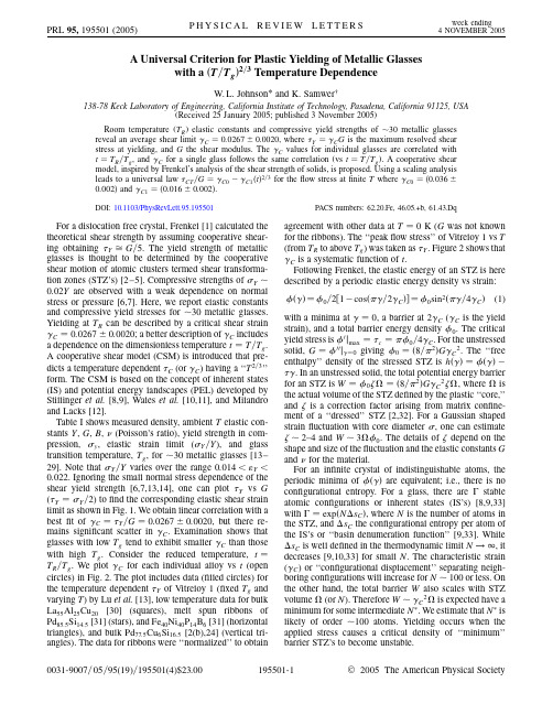
A Universal Criterion for Plastic Yielding of Metallic Glasseswith a T=T g 2=3Temperature DependenceW.L.Johnson*and K.Samwer†138-78Keck Laboratory of Engineering,California Institute of Technology,Pasadena,California91125,USA (Received25January2005;published3November2005)Room temperature(T R)elastic constants and compressive yield strengths of 30metallic glasses reveal an average shear limit C 0:0267 0:0020,where Y C G is the maximum resolved shear stress at yielding,and G the shear modulus.The C values for individual glasses are correlated with t T R=T g,and C for a single glass follows the same correlation(vs t T=T g).A cooperative shear model,inspired by Frenkel’s analysis of the shear strength of solids,is ing a scaling analysis leads to a universal law CT=G C0ÿ C1 t 2=3for theflow stress atfinite T where C0 0:036 0:002 and C1 0:016 0:002 .DOI:10.1103/PhysRevLett.95.195501PACS numbers:62.20.Fe,46.05.+b,61.43.DqFor a dislocation free crystal,Frenkel[1]calculated the theoretical shear strength by assuming cooperative shear-ing obtaining Y G=5.The yield strength of metallic glasses is thought to be determined by the cooperative shear motion of atomic clusters termed shear transforma-tion zones(STZ’s)[2–5].Compressive strengths of Y 0:02Y are observed with a weak dependence on normal stress or pressure[6,7].Here,we report elastic constants and compressive yield stresses for 30metallic glasses. Yielding at T R can be described by a critical shear strain C 0:0267 0:0020;a better description of C includes a dependence on the dimensionless temperature t T=T g.A cooperative shear model(CSM)is introduced that pre-dicts a temperature dependent C(or C)having a‘‘T2=3’’form.The CSM is based on the concept of inherent states (IS)and potential energy landscapes(PEL)developed by Stillinger et al.[8,9],Wales et al.[10,11],and Milandro and Lacks[12].Table I shows measured density,ambient T elastic con-stants Y,G,B, (Poisson’s ratio),yield strength in com-pression, y,elastic strain limit( Y=Y),and glass transition temperature,T g,for 30metallic glasses[13–29].Note that Y=Y varies over the range0:014<"Y< 0:022.Ignoring the small normal stress dependence of the shear yield strength[6,7,13,14],one can plot Y vs G ( Y Y=2)tofind the corresponding elastic shear strain limit as shown in Fig.1.We obtain linear correlation with a bestfit of C Y=G 0:0267 0:0020,but there re-mains significant scatter in C.Examination shows that glasses with low T g tend to exhibit smaller C than those with high T g.Consider the reduced temperature,t T R=T g.We plot C for each individual alloy vs t(open circles)in Fig.2.The plot includes data(filled circles)for the temperature dependent Y of Vitreloy1(fixed T g and varying T)by Lu et al.[13],low temperature data for bulk La55Al25Cu20[30](squares),melt spun ribbons of Pd85:5Si14:5[31](stars),and Fe40Ni40P14B6[31](horizontal triangles),and bulk Pd77:5Cu6Si16:5[2(b),24](vertical tri-angles).The data for ribbons were‘‘normalized’’to obtain agreement with other data at T 0K(G was not known for the ribbons).The‘‘peakflow stress’’of Vitreloy1vs T (from T R to above T g)was taken as Y.Figure2shows that C is a systematic function of t.Following Frenkel,the elastic energy of an STZ is here described by a periodic elastic energy density vs strain: 0=2 1ÿcos =2 C 0sin2 =4 C (1) with a minima at 0,a barrier at2 C( C is the yield strain),and a total barrier energy density 0.The critical yield stress is 0j max c 0=4 C.For the unstressed solid,G 00j 0giving 0 8= 2 G C2.The‘‘free enthalpy’’density of the stressed STZ is h ÿ .In an unstressed solid,the total potential energy barrier for an STZ is W 0 8= 2 G C2 ,where is the actual volume of the STZ defined by the plastic‘‘core,’’and is a correction factor arising from matrix confine-ment of a‘‘dressed’’STZ[2,32].For a Gaussian shaped strainfluctuation with core diameter ,one can estimate 2–4and W 3 0.The details of depend on the shape and size of thefluctuation and the elastic constants G and for the material.For an infinite crystal of indistinguishable atoms,the periodic minima of are equivalent;i.e.,there is no configurational entropy.For a glass,there areÿstable atomic configurations or inherent states(IS’s)[8,9,33] withÿ exp N s C ,where N is the number of atoms in the STZ,and s C the configurational entropy per atom of the IS’s or‘‘basin denumeration function’’[9,33].While s C is well defined in the thermodynamic limit N!1,it decreases[9,10,33]for small N.The characteristic strain ( C)or‘‘configurational displacement’’separating neigh-boring configurations will increase for N 100or less.On the other hand,the total barrier W also scales with STZ volume (or N).Therefore W C2 is expected have a minimum for some intermediate N .We estimate that N is likely of order 100atoms.Yielding occurs when the applied stress causes a critical density of‘‘minimum’’barrier STZ’s to become unstable.The barrier atfinite ,W ,approaches zero as ! C.It is easily shown that 0 (barrier energy density atfinite ! C)decreases as 0 Cÿ 3=2while the shear modulus(atfinite )G Cÿ 1=2.The strain differ-ence between the energy minimum and barrier configura-tion(saddle point)scales as Cÿ 1=2as ! C. Mechanical instability of the STZ at C takes the form of a ‘‘fold catastrophe’’[11,34].For ! C,the parameters W 0 , ,and G ,are related by the scaling law0 = G 2 R 1=4;so that W G C 2 ;(2)where R is the‘‘fold ratio.’’Wales et al.[11,34]have shown that,for binary Lennard Jones(LJ)glasses (256atoms)and liquid salt clusters(71atoms),this scaling relation holds on average,even far from C.For the Frenkel landscape of Eq.(1),R actually varies from1=4to 2=32as varies from C down to0.Analysis of simulation results[12]for shear induced destabilization of individual IS’s of a500atom LJ glass shows that Eq.(2) is obeyed(within10%)over0< < C.Assuming scal-ing holds on average:W W0 T Cÿ = C 3=2 0 Cÿ = C 3=2 4RG0TC2Cÿ = C 3=2 ;(3) where G0T is the shear modulus of the unstressed glass which includes a weak dependence on T(Debye-Gru¨neisen thermal expansion)for afixed glass configuration.The scaling law holds for any function for which d2 =d 2is analytic around the inflection point.At finite T and applied ,thermal strainfluctuations will carry the system over the barrier W .For plasticflow to occur on a given time scale(or strain rate_ ),the rate of barrier crossing must reach a critical value comparable to_ .UsingTABLE I.Summary of data on alloy compositions and properties used in this Letter.PropertyAlloy Y)G B y T g(g=cc)(GPa)(GPa)(GPa) (GPa)(K) y=Y Ref.1.Zr41:2Ti13:8Ni10Cu12:5Be22:5 5.99534.1114.10.352 1.866180.0196[13–15]97.235.9111.20.354 1.856130.01902.Zr48Nb8Ni12Cu14Be18 6.793.934.31180.367 1.956200.0208[15]3.Zr55Ti5Cu20Ni10Al10 6.6285311180.375 1.636250.0192[15]4.Zr57:5Nb5Cu15:4Ni12Al10 6.584.730.8117.60.379 1.586630.0187[15]5.Zr55Al19Co19Cu76.2101.737.6114.90.352 2.27330.0216[16]6.Pd40Cu30Ni10P209.289234.5151.80.399 1.725930.0187[17]7.Pd40Cu30Ni10P209.2892331460.394 1.725930.0187[18]8.Pd40Cu30Ni10P209.309235.8144.70.394 1.755950.0190[17]9.Pd60Cu20P209.789132.31670.409 1.706040.0187[15]10.Pd40Cu40P209.309333.21580.402 1.755480.0188[15]11.Ni45Ti20Zr25Al10 6.4109.340.2129.60.359 2.377910.0217[19]12.Ni40Ti17Zr28Al10Cu5 6.48127.647.3140.70.349 2.598620.0203[19]13.Ni60Nb35Sn58.64183.766.322670.385 3.858850.0210[20]14.Ni60Sn6 Nb0:8Ta0:2 349.24161.359.411890.357 3.508750.0217[16]15.Ni60Sn6 Nb0:6Ta0:4 349.80163.760.1197.60.361 3.588820.0219[16]16.Cu64Zr368.079234104.30.352 2.07870.0217[21]17.Cu46Zr547.6283.530.0128.50.391 1.406960.0168[22]18.Cu46Zr42Al7Y57.2384.631104.10.364 1.607130.0189[23]19.Pd77:5Cu6Si16:510.489.731.81660.409 1.55500.0167[24]20.Pt60Ni15P2515.796.133.82020.420 1.44880.0146[25]21.Pt57:5Cu14:7Ni5P22:815.295.733.4243.20.434 1.454900.0151[26]22.Pd64Ni16P2010.191.932.71660.405 1.554520.0169[24]23.MgGd10Cu25 4.0449.118.646.30.320.984280.020[16]55Al25Cu10Ni5Co5 6.041.915.644.20.3420.854300.0203[15]25.Ce70Al10Ni10Cu10 6.6730.311.5270.3130.653590.0215[27]26.Cu50Hf43Al711.011342132.80.358 2.27740.0195[16]27.Cu57:5Hf27:5Ti159.9110337.3117.50.356 1.947290.0188[16]28.Fe61Mn10Cr4Mo6Er1C15B6 6.89193751460.280 4.168700.0216[28]29.Fe53Cr15Mo14Er1C15B6 6.92195751800.32 4.28600.0215[28]30.Au49:5Ag5:5Pd2:3Cu26:9Si16:311.674.426.5132.30.406 1.204050.0141[29]31.Au55Cu25Si2012.269.824.6139.80.417 1.003480.0143[29]an attempt frequency !0requiresyielding rate !0exp ÿW =kT C _ ;(4)with C a dimensionless constant of order unity,and thus W =kT ÿln C _ =!0 f 4RG 0T C 2 C 0ÿ CT = C 3=2 g =kT:(5)Here, C 0is the yield stress at T 0,while CT is at finiteT .One obtainsCT C 0ÿ C 0 kT ln !0=C _= 4RG 0T C 2 2=3:(6)At T T g and 0,the barrier is W 0 T g4RG 0Tg C 2 .If T g itself is defined by a critical barrier crossing rate due to fluctuations,one obtains W 0 T g T g ,with constant.This yieldsW ;Tg T g C ÿ = C 3=2:(7)Equation (6)for the yield stress becomesCT C 0ÿ C 0 k= ln !0=C _G 0T =G 0Tg 2=3t 2=3;(8)where t T=T g .The factor (G 0T =G 0Tg )incorporates theweak dependence of G on the thermal expansion of a fixed glass configuration.G 0T has been experimentally deter-mined [15,18]to be a linear function of T .For Vitreloy 1[15],one finds dG 0T =dT 4 10ÿ3 GPa =K with G 0 37GPa at 0K.Since the thermal expansion coefficient will drop at very low T ,one obtains an upper bound for the fractional change in G 0T =G 0Tg from 0K to T g as max T g =G 0 dG 0T =dT 0:07.Similarly,we estimate max 0:11for Pd 40Ni 40P 20[18].The t dependence of G 0T =G 0Tg gives a maximum correction to the second term in Eq.(8)at t 1(near T g )of order 5%–7%.The logarithmic term in Eq.(8)involves !0and is estimated to be the frequency of shear phonon of nm wavelength ( 1013Hz ).With typical strain rates (in yielding experiments)of10ÿ2–10ÿ4s ÿ1,we have ln !0=C _30.An order of magnitude change in either !0or _changes the loga-rithmic term by 5%.The dependence of CT on T is thus dominated by the t 2=3term.The dotted curve in Fig.2was obtained using Eq.(8)(square bracket taken as a constant)to ‘‘fit’’the depen-dence of CT at T R (fixed T )and varying T g for the 30metallic glasses (open circles)and the t dependence of individual alloys (filled symbols).This fit gives Y =G C 0 C 1t m where C 0 0:036 0:002, C 1 0:016 0:002,and m 0:62 0:2.Equation (8)explains both the T dependence of Y for all individual amorphous alloys and the ‘‘T g dependence’’for 30glasses at fixed T R with an exponent ‘‘m ’’consistent (within error)with the predicted value ‘‘2=3.’’The coefficients C 0and C 1are approxi-mately universal constants.The present classical model is expected to break down at very low T .Low T data shown in the inset of Fig.2suggest ‘‘quantum effects’’on yielding when shear phonon modes ‘‘freeze out’’at very low T .For the CSM,the elastic response of an STZ is nonlinear as increases from 0to C .The actual critical strain at C is not CT =G (as in experiments),but rather CT =2G with the factor =2arising from nonlinear elasticity.The role of nonlinear elasticity and nonaffine atomic displace-ments in the shear response of an STZ has been recently discussed [35,36].In both the Frenkel model and simula-tions [35],the compliance at finite stress,G ÿ1,diverges at C .Experimentally,one measures yield stress,notstrain,FIG.2(color online).Experimental shear strain at yielding( Y =G )vs t T=T g .Small open circles show results at room temperature on 30alloys of varying T g .Solid symbols show the t dependence of Y =G for various individual alloys as indicated.The reader is referred to the text for references anddetails.FIG.1.Experimental shear stress at yielding, Y Y =2vs shear modulus G at room temperature for 30bulk metallic glasses.so the experimental C at yield underestimates the actual strain of the STZ.Further,the macroscopic material com-prises a statistical distribution of STZ’s with distributed values of G and C varying with location and orientation. Yielding is expected when a critical fraction of unstable STZ’s results in global instability.In conclusion,plastic yielding of metallic glasses at T R is roughly described by an average elastic shear limit criterion, Y C G,where G is the shear modulus of the unstressed glass,and C 0:0267 0:0020.Closer analysis reveals that C depends on t T=T g.A CSM inspired by Frenkel’s work and recent molecular dynamics simulations is developed to explain these empiricalfind-ings.Yielding is treated as a fold catastrophe obeying a scaling law W = G 2 R.Applied on average, this scaling law leads to a‘‘t2=3law,’’ CT=G C0ÿ C1 t 2=3,forflow stress of metallic glasses where C0and C1are weakly material dependent.Afit to all experimental data yields C0 0:036 0:002 , C1 0:016 0:002 ,and an exponent m 0:62 0:2.A similar derivation of the‘‘T2=3’’law has appeared in the literature on yielding in crystals[37].Gaunt also derived a similar law for thermally activated domain wall motion in disordered magnets[38].To the extent that plastic yielding in nonmetallic glasses(oxides,molecular glasses,etc.)is a fold catastrophe,one might expect Eq.(8) to be valid more generally although C0may vary.The present CSM model may establish a basis for a broader understanding of glass physics.W.L.J.acknowledges the Defence Advanced Re-search Projects Agency(DARPA-DSO),ARO Grant No.DAAD19-01-1-0525and the National Science Foundation for providing support under the Caltech MRSEC program.K.S.acknowledges the support of the DFG under Grant No.SFB602and the Leibniz Program.*Electronic address:wlj@†Permanent address:I.Physik Institute,University of Goettingen,Goettingen,Germany.[1]J.Frenkel,Z.Phys.37,572(1926);see also A.Kelly,Strong Solids(Clarendon Press,Oxford,1973),2nd ed.[2](a)A.S.Argon,Acta Metall.27,47(1979);(b)A.Argonand L.T.Shi,Acta Metall.31,499(1983).[3] F.Spaepen,Acta Metall.25,407(1977);see also P.S.Steif,F.Spaepen,and J.W.Hutchinson,Acta Metall.30, 447(1982).[4]M.L.Falk and nger,Phys.Rev.E57,7192(1998).[5]nger,Phys.Rev.E70,041502(2004).[6]See P.E.Donovan,Acta Metall.37,445(1989);J.J.Lewandowski and P.Lowhaphandu,Philos.Mag.A82, 3427(2002).[7]J.Lu and G.Ravichandran,J.Mater.Res.18,2039(2003).[8] F.H.Stillinger and T.A.Weber,J.Chem.Phys.88,7818(1988);Science267,1935(1995).[9]P.G.Debenedetti and F.H.Stillinger,Nature(London)410,259(2001).[10]J.P.K.Doye and D.J.Wales,J.Chem.Phys.116,3777(2002).[11] D.J.Wales,Science293,2067(2001).[12] D.L.Malandro and cks,J.Chem.Phys.110,4593(1999);also107,5804(1997).[13]J.Lu,G.Ravichandran,and W.L.Johnson,Acta Mater.51,3429(2003).[14]H.Bruck,T.Christman,A.J.Rosakis,and W.L.Johnson,Scr.Metall.Mater.30,429(1994);also F.Szuecs,C.P.Kim,and W.L.Johnson,Acta Mater.49,1507(2001).[15]Y.Zhang,D.Q.Zhao,R.J.Wang,and W.H.Wang,ActaMater.51,1971(2003);also W.H.Wang,C.Dong,andC.H.Shek,Mater.Sci.Eng.,R44,45(2004).[16]J.Kang,M.L.Lind,H.C.Yim,and W.L.Johnson(un-published).[17]U.Harms,O.Jin,and R.B.Schwarz,J.Non-Cryst.Solids317,200(2003).[18]N.Nishiyama,A.Inoue,and J.Z.Jiang,Appl.Phys.Lett.78,1985(2001).[19] D.H.Xu,G.Duan,and W.L.Johnson,Acta Mater.52,3493(2004).[20]H.Choi-Yim,D.H.Xu,and W.L.Johnson,Appl.Phys.Lett.82,1030(2003).[21] D.H.Xu, B.Lohwongwatana,G.Duan,and W.L.Johnson,Acta Mater.52,2621(2004).[22]G.Duan,D.H.Xu,and W.L.Johnson,Phys.Rev.B71,224208(2005).[23] D.H.Xu,G.Duan,and W.L.Johnson,Phys.Rev.Lett.92,245504(2004).[24] B.Golding,B.G.Bagley,and F.S.L.Hsu,Phys.Rev.Lett.29,68(1972).[25]H.S.Chen,J.T.Krause,and E.Coleman,J.Non-Cryst.Solids18,157(1975).[26]J.Schroers and W.L.Johnson,Appl.Phys.Lett.84,3666(2004);also Phys.Rev.Lett.93,255506(2004). [27] B.Zhang,M.X.Pan,Q.Zhao,and W.H.Wang,Appl.Phys.Lett.85,61(2004).[28]V.Ponnambalam,S.J.Poon,and G.J.Shiflet,J.Mater.Res.19,3046(2004);19,1320(2004);(private commu-nication).[29]J.Schroers, B.Lohwongwatana, A.Peker,and W.L.Johnson,Appl.Phys.Lett.87,061912(2005).[30]S.Takeuchi,T.Kakegawa,T.Hashimoto,A.-P.Tsai,andA.Inoue,Mater.Trans.,JIM41,1443(2000).[31]V.Z.Bengus,E.D.Tabachnikova,P.Duhaj,and V.Ocelik,Mater.Sci.Eng.A226–228,823(1997).[32]J.D.Eshelby,Proc.R.Soc.A241,376(1961).[33]M.S.Shell,P.G.Debenedetti,Nave,and F.Sciortino,J.Chem.Phys.118,8821(2003).[34]T.V.Bogdan and D.J.Wales,J.Chem.Phys.120,11090(2004).[35] C.Maloney and A.Lemaitre,Phys.Rev.Lett.93,195501(2004).[36] A.Tanguy,J.P.Wittmer,F.Leonforte,and J.L.Barrat,Phys.Rev.B66,174205(2002).[37]U.F.Kocks,A.S.Argon,and M.F.Ashby,Prog.Mater.Sci.19,1(1975).[38]P.Gaunt,Philos.Mag.B48,261(1983);Philos.Mag.34,775(1976).。
- 1、下载文档前请自行甄别文档内容的完整性,平台不提供额外的编辑、内容补充、找答案等附加服务。
- 2、"仅部分预览"的文档,不可在线预览部分如存在完整性等问题,可反馈申请退款(可完整预览的文档不适用该条件!)。
- 3、如文档侵犯您的权益,请联系客服反馈,我们会尽快为您处理(人工客服工作时间:9:00-18:30)。
a r X i v :0805.4685v 1 [n u c l -t h ] 30 M a y 2008Low-density limit as a test for the models of complicatedprocesses in the nucleiV.I.Nazaruk Institute for Nuclear Research of the Academy of Sciences of Russia,60th October Anniversary Prospect 7a,117312Moscow,Russia.*Abstract We propose to use the branching ratio of channels of free-space hadron-nucleon inter-action as a test in the construction and verification of the models of complicated processes in the nuclei.The particle self-energy and amplitudes of subprocesses are studied as well.PACS:24.10.-i,13.75.Cs Keywords:low-density limit,diagram technique,decay,self-energy*E-mail:nazaruk@inr.ruLet us consider a free-space decay a→π0¯n,for example,¯Λ→π0¯n.For a decay in the medium the annihilationa→π0+¯n→π0+M(1)and scatteringa→π0+¯n→π0+¯n(2)channels take place.Here M are the annihilation mesons,¯n→M and¯n→¯n imply the annihilation and scattering of¯n in the medium,respectively.In[1,2]it was shown that the phenomenoligical model based on optical potential does not describe the decay channel(1)as well as the total decay probability of the a-particle.It describes the channel(2)only.This is because the equation f=i|T fi|2≈2Im T ii cannot be used for the essentially non-unitary S-matrix.This is also true for the more complicated decays and reactions[2].In this connection we continue consideration of some aspects of unitary models of multistep processes in the nuclear matter.LetΓa,Γs andΓt be the widths of the decays(1),(2)and the total width of the decay a→π0¯n in the medium,respectively.(For a decay in nuclear matter Γs≈0since the¯n annihilates in a timeτa∼1/Γ,whereΓis the annihilation width of¯n in the medium.)We calculate theΓa,Γt and the branching ratio of channels.In the low-density approximation[3,4]the expressions for the branching ratio of channels and particle self-energy have a clear physical meaning(we emphasize this fact),which enables one to verify and correct the model.It is shown that the models of realistic processes in the nuclei should reproduce the branching ratio of channels of the corresponding free-space hadron-nucleon interactions. This can be considered as necessary condition for the correct model construction.The results obtained for the decay a→π0¯n are generalized to the decaya→b+c(3) and reactiona+N→b+c(4) followed by elastic and inelastic c-medium interactions.We focus on the intermediate-state interaction of the¯n(c-particle)and so theπ0-medium(b-medium)interaction is inessential for us.(In a recent paper[5],the similar program has been realized for the n¯n transitions[6-8]in the medium followed by annihilation:n→¯n→M.This is a simplest process involving the intermediate-state interaction since the n¯n transition vertex corresponds to2-tail diagram.In this paper the consideration is generalized to the processes(3)and(4).)We calculate the width of the decay(1).Our plan is as follows.1)First of all we construct and study the simplest process model sutable to the concrete calculations.2)In the framework of this model we calculate the values listed above.In order to construct the model correctly,we considerfirst the free-space¯n N annihilation (see Fig.1a)and the process on a free nucleona+N→π0+¯n+N→π0+M,(5)shown in Fig.1b(the free-space subprocess).The amplitude of free-space¯n N annihilation M a is defined as<M|T exp(−i dx H¯n N(x))−1|¯n N>=N a(2π)4δ4(p f−p i)M a.(6) Here H¯n N is the Hamiltonian of the¯n N interaction,N a includes the normalization factors of the wave functions.M a involves all the¯n N interactions followed by annihilation including the ¯n N rescattering in the initial state.Figure1:a Free-space¯n N annihilation.b Free-space reaction a+N→π0+¯n+N→π0+M.We write the formulas corresponding to Fig.1b.The interaction Hamiltonian isH I=H d+H¯n N,(7)H d=g¯Ψ¯nΦ∗Ψa+H.c.,(8) where H d is the Hamiltonian of the decay a→π0¯n.In the following the antineutron and a-particle are assumed non-relativistic and spinless.In the lowest order in H d the amplitude of the process(5)is given byM1b=gGM a,(9)1G=where p and q are the4-momenta of the a-particle andπ0,respectively,m is the antineutron mass,M a is given by(6).Since M a contains all the¯n N interactions followed by annihilation, the antineutron propagator G is bare.Consider now the decay(1)(see Fig.2a).The background a-particle potential is included in the wave function of a-particleΨa(x).The interaction Hamiltonian has the formH I=H d+H,(11)where H is the Hamiltonian of the¯n-medium interaction.In the lowest order in H d the amplitude of the process,M2a,is uniquely determined by the Hamiltonian(11):M2a=gGM m a.(12) The amplitude of the¯n-medium annihilation M m a is given by<f|T exp(−i dx H(x))−1|0¯n p−q>=N(2π)4δ4(p f−p i)M m a(13) (compare with(6)).Here|0¯n p−q>and<f|are the states of the medium containing the¯n with the4-momentum p−q and annihilation products,respectively;N includes the normalization factors of the wave functions.Figure2:a Decay a→π0+¯n→π0+M in nuclear matter.The antineutron annihilation is shown by a circle.b The same as a,but the antineutron propagator is dressed(see text).The definition of the annihilation amplitude M m a through Eqs.(13)is natural.If the number of particles of medium is equal to unity,Eq.(13)goes into(6).The antineutron annihilation widthΓis expressed through M m a(see Eq.(20)).M m a involves all the¯n-medium interactions followed by annihilation including the antineutron rescattering in the initial state.Due to this, the propagator G is bare.As in(9),the antineutron self-energyΣ=0since the interaction, which can generateΣ,is involved in M m a.If the Hamiltonian H is expressed through the¯n N-and NN-interactions,the amplitude M m a contains in medium¯n N-amplitudes and dressed propagators.In this case the following condition should be fulfilled:ifρ→0,the propagator is not dressed.However,our purpose is to study the general features of the simplest model suitable to the concrete calculations and not the medium effects.On this reason we consider the model(12)which contains the block M m a corresponding to the observable values.We would like to emphasize this paragraph.Our results(Eqs.(29)-(35))may not depend on the model of the block M m a.However,for the concrete calculations given in this paper,the fact that the propagator is bare is principal and so we study this point in ing the same Hamiltonian(11),we try to construct the model with the dressed propagator(see Fig.2b).Let U¯n be the optical potential of¯n.DenoteV=Re U¯n.(14)We recall the Hamiltonian H involves all the¯n-medium interactions.In the Hamiltonian H we separate out the real potential V:H=V¯Ψ¯nΨ¯n+H′(15)and include it in the antineutron Green function1G d=G+GV G+...=(The formal expression for the dressed propagator should contain the annihilation loops as well.In this case the statements given in pp.(1)and(2)are only enhanced.A particle self-energy should be considered in the context of the concrete problem.The dressed propagator arises naturally if V and H′are the principally different interactions and vertex function does not depend on V.In our problem one and the samefield generatesΣand M m a.)(4)Equations(16)and(17)mean that the annihilation is turned on upon forming of the self-energy partΣ=V(after multiple rescattering of¯n).This is counter-intuitive since at the low energies[9-11]σag2G2Γ,(20)2q0(2π)3whereΓis the annihilation rate of the¯n with the4-momentum p−q.The corresponding amplitude M m a is given by(13).Up to this point the low-density limit has been not used.The number of exchanges with the medium or particle,which appears in(16),is very important but unobservable value.In particular,it is responsible for the particle self-energy and process suppression by the potential V.The low-density approximation enables one to verify directly the condition(19).Indeed,in the low-density approximationΓ=vρσa andΓa= d q F1σa,(21)F1=g2G2vρ(2π)4giT02Im M3=Γt,(24)1Γt= dqF(q)σa(q)q0,(28) q20=q2+m2π.In the differential formdΓa/dqσt.(29) In a similar manner,one obtainsdΓs/dqσt.(30)We consider the free-space decay(3).Let for the decay in the medium the inelastica→b+c→b+x(31)and elastica→b+c→b+c(32)interactions of the c-particle take place.Here c→x and c→c imply the reaction induced by c-particle and scattering of c-particle in the medium,respectively.LetΓr andΓs be the widths of decays(31)and(32),respectively;Γt=Γr+Γs.With the replacementΓa→Γr and σa→σr,the relations(27)-(30)describe the decay channels(31)and(32).For the process(4)in the medium instead of(31)and(32)we consider the reactions on the nucleon of the medium:a+N→b+c→b+x(33)anda+N→b+c→b+c.(34)In this case the similar relations take place as well.The corresponding changes in F are minimum and non-principal.For example,for the channels(33)and(34)we getdσm r/dq,(35)σswhereσm r andσm s are the cross sections of the reactions(33)and(34),respectively.Relations(27)-(30)are directly connected with the experimental branching ratiosσa/σt and σs/σt(see(19)).The similar statements are also true for the decays like(31),(32)and reactions (33),(34)in the medium.The nuclear medium changes the amplitudes[12]and branching ratio of channels[13]in hadron-nucleon interactions.Besides,the strong antineutron absorption takes place.Due to this,at the nuclear densitiesΓa/Γt≈1.However,ifρ→0,the relations (27)-(30)should be reproduced.The definition of annihilation amplitude through Eqs.(6)and(13)is natural since it corresponds to the observable values.In that event the intermediate particle propagator is bare and relation(19)is reproduced.(This does not contradict to well-known results[14-18] becauseΣshould be considered in the context of the concrete problem.)Certainly,we do not argue that above-considered scheme is the only possible model.This is clear even from Eq.(18).Besides,the Hamiltonian H can be concretized.We argue only the following:once the amplitudes are defined by(6)and(13)(which is natural),the propagator is bare;the free-space processes shown in Fig.1and the experimental branching ratio of channels like(19)are reproduced.In fact,the relations like(29),(30)and(35)should be fulfilled for any process model and can be considered as necessary condition for the correct model construction.References[1]V.I.Nazaruk,Mod.Phys.Lett.A21(2006)2189;V.I.Nazaruk,Proceedings of the9thInternational Conference on Low Energy Antiproton Physics(LEAP’05),Bonn,Germany 2005,edited by D.Grzonka,R.Czyzykiewich,W.Oelert,T.Rozek,P.Winter,AIP Conf.Proc.796(2005)180.[2]V.I.Nazaruk,Eur.Phys.J.A.31(2007),177.[3]C.B.Dover,J.Hufner and R.H.Lemmer,Ann.Phys.66,248(1971).[4]J.Hufner,Phys.Rep.21,1(1975).[5]V.I.Nazaruk,Eur.Phys.J.C53,573(2008).[6]S.L.Glashow,preprint HUTP-79/A059(Harvard,1979).[7]R.N.Mohapatra and R.E.Marshak,Phys.Rev.Lett.44,1316(1980).[8]V.I.Nazaruk,Phys.Rev.C58,R1884(1998).[9]T.Kalogeropoulos and G.S.Tzanakos,Phys.Rev.D22,2585(1980).[10]G.S.Mutchler et al.,Phys.Rev.D38,742(1988).[11]W.Bruckner et al.,preprint CERN-EP/89-105(Geneve1989).[12]T.Ericson and W.Weise,Pions and Nuclei(Clarendon Press,Oxford,1988).[13]V.I.Nazaruk,Phys.Lett.B218,291(1989).[14]P.Fernandez de Cordona and E.Oset,Phys.Rev.C46,1697(1992).[15]L.Alvarez-Ruso,P.Fernandez de Cordoba and E.Oset,Nucl.Phys.A606,407(1996).[16]A.Bieniek et al.,Phys.Lett.B526,329(2002).[17]M.Benmerrouche et al.,Phys.Rev.C39,2339(1989).[18]V.K.Madas,L.Roka and E.Oset,Phys.Rev.C71,065202(2005).。