计量经济学实验报告英文版
EViews计量经济学实验报告-多重共线性的诊断与修正的讨论
实验题目 多重共线性的诊断与修正一、实验目的与要求:要求目的:1、对多元线性回归模型的多重共线性的诊断;2、对多元线性回归模型的多重共线性的修正。
二、实验内容根据书上第四章引子“农业的发展反而会减少财政收入”,1978-2007年的财政收入,农业增加值,工业增加值,建筑业增加值等数据,运用EV 软件,做回归分析,判断是否存在多重共线性,以及修正。
三、实验过程:(实践过程、实践所有参数与指标、理论依据说明等)(一)模型设定及其估计经分析,影响财政收入的主要因素,除了农业增加值,工业增加值,建筑业增加值以外,还可能与总人口等因素有关。
研究“农业的发展反而会减少财政收入”这个问题。
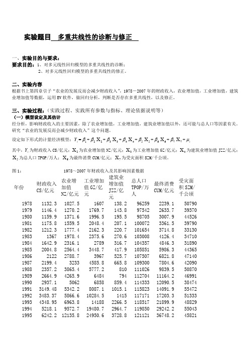
设定如下形式的计量经济模型:i Y =1β+2β2X +3β3X +4β4X +5β5X +6β6X +7β7X +i μ其中,i Y 为财政收入CS/亿元;2X 为农业增加值NZ/亿元;3X 为工业增加值GZ/亿元;4X 为建筑业增加值JZZ/亿元;5X 为总人口TPOP/万人;6X 为最终消费CUM/亿元;7X 为受灾面积SZM/千公顷。
图1: 1978~2007年财政收入及其影响因素数据年份财政收入CS/亿元 农业增加值NZ/亿元 工业增加值GZ/亿元 建筑业增加值JZZ/亿元总人口TPOP/万人最终消费CUM/亿元受灾面积SZM/千公顷 1978 1132.3 1027.5 1607 138.2 96259 2239.1 50790 1979 1146.4 1270.2 1769.7 143.8 97542 2633.7 39370 1980 1159.9 1371.6 1996.5 195.5 98705 3007.9 44526 1981 1175.8 1559.5 2048.4 207.1 100072 3361.5 39790 1982 1212.3 1777.4 2162.3 220.7 101654 3714.8 33130 1983 1367 1978.4 2375.6 270.6 103008 4126.4 34710 1984 1642.9 2316.1 2789 316.7 104357 4846.3 31890 1985 2004.8 2564.4 3448.7 417.9 105851 5986.3 44365 1986 2122 2788.7 3967 525.7 107507 6821.8 47140 1987 2199.4 3233 4585.8 665.8 109300 7804.6 42090 1988 2357.2 3865.4 5777.2 810 111026 9839.5 50870 1989 2664.9 4265.9 6484 794 112704 11164.2 46991 1990 2937.1 5062 6858 859.4 114333 12090.5 38474 1991 3149.48 5342.2 8087.1 1015.1 115823 14091.9 55472 1992 3483.37 5866.6 10284.5 1415 117171 17203.3 51333 1993 4348.95 6963.8 14188 2266.5 118517 21899.9 48829 1994 5218.1 9572.7 19480.7 2964.7 119850 29242.2 55043 19956242.2 12135.8 24950.6 3728.8 12112136748.2458211996 7407.99 14015.4 29447.6 4387.4 122389 43919.5 46989 1997 8651.14 14441.9 32921.4 4621.6 123626 48140.6 53429 1998 9875.95 14817.6 34018.4 4985.8 124761 51588.2 50145 1999 11444.08 14770 35861.5 5172.1 125786 55636.9 49981 2000 13395.23 14944.7 40036 5522.3 126743 61516 54688 2001 16386.04 15781.3 43580.6 5931.7 127627 66878.3 52215 2002 18903.64 16537 47431.3 6465.5 128453 71691.2 47119 2003 21715.25 17381.7 54945.5 7490.8 129227 77449.5 54506 2004 26396.47 21412.7 65210 8694.3 129988 87032.9 37106 2005 31649.29 22420 76912.9 10133.8 130756 96918.1 38818 2006 38760.2 24040 91310.9 11851.1 131448 110595.3 41091 2007 51321.78 28095 107367.2 14014.1 132129 128444.6 48992利用EV 软件,生成i Y 、2X 、3X 、4X 、5X 、6X 、7X 等数据,采用这些数据对模型进行OLS 回归。
《计量经济学》实训报告内容

进一步检查是否存在异方差,倘若存在,更改权重 (例如,残差项平方的倒数作为权重)
2019/2/14 4
第二次实训内容:对时间序列数据 进行线性回归
• 基本步骤
建立数据文件 Quick-Equation Estimation-输入计量模型
2019/2/14
5
• 如何防止多重共线性?
相关性分析(View-Covariance Analysis) 解决方法:排除变量法、差分法(在时间序列 数据、面板数据中使用)
2019/2/14
6
• 如何防止序列相关性?
在回归方程中加入ar(1)、ar(2)……,检验D.W. 值是否接近于2
2019/2/14
7
第三次实训内容:对面板数据进行 线性回归
• 基本步骤
建立数据文件
如何防止多重共线性?略。
一般不考虑异方差性和序列相关性。
2019/2/14
8
Estimate,在Specification中输入被解释变量 (加一个问号),在cross-section中选择 random;在Common coefficents中各自变 量(每个自变量后面加一个问号,并且用空格 隔开),点击确定。 固定效应和随机效应的选择:ViewFixed/Random Effect Testing-Correlated Random Effects-Hausman Test,倘若 Cross-section random的伴随概率小于0.1, 那么运用固定效应,否则运用随机效应。
实验报告计量经济学

计量经济学实验报告书实验二、实验开设对象本实验的开设对象为《计量经济学》课程的学习者,实验为必修内容、实验目的实验二、掌握计量经济学多元模型的建立,模型形式的设定,模型拟合度、t检验和F 检验判断过程;三、实验环境微型计算机(要求必须能够连接In ternet,且安装有Eviews6.0软件。
)四、实验成果根据所给定的范例数据和要求,利用Eviews6.0软件对其进行分析和处理,并撰写实验报告。
Workflle U*mTLEDViaw | Prc-c d Oku"^1 | P-ranl N HIWH rra«x«DW BL *▼ | I Sia-r^ Tranap-aiiB E-drlI3T ■3MB ■工:xi 沁4b3-¥ XtX2IP 阴rn 丁也电niSb0.6534101985175 479724.11729 0.057131inn. IH ^I I :史Nfl 昭却* n 1*寻 1SB7 壬 g B2S£I7-2-4.13-112 ” D 日皿N 10BS2J.17 3J9 0.74200<5 I 總HP 71. 1 HURT口 TTiflHR?23:7j2S3:21.7S-103 D.7487B6-IB9-I £55 5541 2a.344*ie 0.7300821R>Ri77nn )npeii in 口 口 丁7■口sji-4 鬧 13 S1437 D.76B2&71^94 3&3 E7&& 17-93 17^ 0 61320BTRiR ■刍Hon R,Df»ri in :1:7口□ 口 riAHH433 03:2H 1占:&也斗出-IBBT 4眄 44&Z is.33333 0.9171051DEII1SiD 1 HUA ia CHI 孑pp □ 071斗口 Tis.ess«e 1.006117ZDDD &丁口 48TS 1庁方"5昌 1.069^627DD1 & 1 U 74+4 13 U7Q3Q 1 了曰□斗12002 67& 4-3^2 Ifi 12>D€2 1.^845072QQ3 T33 0&54is1.5301963DD4"iiI 葩 I Grc-up: LflN RJ I LE J D WcdJil*: (JNTTTLE&rLinfcrtiaKT'. J |optic-rii Jupdata Ad-dTri^L ・・l <oraph: UMTTT L ED Wnrkfii ■:: <jNTin"LED::Urrtrt:l«d i,i PtCTc|obj«ct j|^!Print|HMnBCarjpK Opliion-Si—Grap*! typ«-OetalwiSrapH dat-a:Fit Ihnesi!Axi^i tKJV iJdrr :1^1^ ■|~s l li^«■C^K£i[U¥|X1O[k&*朗X21333137?D146 |23 -IBD-IS ft fii 122-41^3-4 1S6.773324 OB&^D0 *£^41Qi^as175.470724 317230EW134fosei laa.teaa24 2D&&1 C €441251537 206.SJ9724 13-112 G1>QS8226.273224 1734&G.742<XM1339 231 aes?22 3G7B40 73511-321>E190237.2836S1.751D30.74^76619912S5.!ifiJ12D 3G4-SB0.73OTB21992286.390613 9DB3D0 7707171393 32i 90531E 519BT0 TBAZUj?363.27C517.BB174 O.S132tlS1995390.SO9S-IE 32DDE.0W7M11995433.932515.BZ244Q WB Mfi19S7ilGgjdiSS15.233BE0/9171Miggg50 1.385 J15.DG7B90 97H4A1199953J.9-392 1 CMW1172000 575.-337915.3E55412001 fiig n7ddldi B7-D59 1 2W4152002 570.J12215.12953 1 ML4W72003 733.CJC5d!15.424BD% si^iggzog 4in* _ b回Groupi UrrrnLED Worwila UNrTTTLEDiiUrt4iecr>. . 5 X[vfcaw] [ Ptlnt] M«n・]rriMM_| [ifWi. F J [ WDrt[Tkiam口■■[lE曰5M(I IL'L;. Grnun: UNTril l O Warlcf ik< UNTITI. ri? IJnfcrilwiA,「召斫i凶。
eviews计量经济学实验报告

eviews计量经济学实验报告EViews计量经济学实验报告引言计量经济学是经济学领域中的一个重要分支,它运用数学、统计学和计量学的方法来分析经济现象。
EViews是一个常用的计量经济学软件,它提供了丰富的数据分析和模型建立工具,被广泛应用于学术研究和实际经济分析中。
本实验报告将利用EViews软件进行计量经济学实验,以探讨经济现象并得出相关结论。
实验目的本实验旨在利用EViews软件对某一经济现象进行实证分析,通过建立相应的计量经济模型,对经济现象进行量化分析,并得出相关结论。
实验步骤1. 数据收集:首先,我们需要收集与所研究经济现象相关的数据,包括时间序列数据和横截面数据等。
这些数据可以来自于官方统计机构、学术研究机构或者自行收集整理。
2. 数据预处理:接下来,我们需要对收集到的数据进行预处理,包括数据清洗、缺失值处理、异常值处理等,以确保数据的质量和完整性。
3. 模型建立:在数据预处理完成后,我们可以利用EViews软件建立计量经济模型,包括回归分析、时间序列分析、面板数据分析等,以探讨经济现象的内在规律和影响因素。
4. 模型估计:建立模型后,我们需要对模型进行参数估计,得到模型的具体参数估计值,并进行显著性检验和模型拟合度检验,以验证模型的可靠性和有效性。
5. 结果分析:最后,我们将对模型估计结果进行分析,得出与经济现象相关的结论,并对实证分析结果进行解释和讨论。
实验结论通过以上实验步骤,我们得出了关于某一经济现象的实证分析结果,并得出了相关的结论。
这些结论对于理解经济现象的内在规律和制定经济政策具有重要的参考价值。
总结EViews计量经济学实验报告通过利用EViews软件进行实证分析,对经济现象进行了深入探讨,并得出了相关结论。
这些结论对于经济学研究和实际经济分析具有重要的理论和实践意义,为我们深入理解经济现象和推动经济发展提供了重要的参考依据。
EViews软件的应用为我们提供了一个强大的工具,帮助我们更好地理解和分析经济现象,为经济学领域的研究和实践提供了重要的支持和帮助。
计量经济学实验报告

学生实验报告学生姓名学号组员:实验项目EVIEWS的使用√必修□选修√演示性实验√验证性实验□操作性实验□综合性实验实验地点管理模拟实验室实验仪器台号指导教师实验日期及节次一、实验目的及要求1、目的会使用EVIEWS对计量经济模型进行分析2、内容及要求(1)对经典线形回归模型进行参数估计、参数的检验与区间估计,对模型总体进行显著性检验;(2)异方差的检验及其处理;(3)自相关的检验及其处理;(4)多重共线性检验及其处理;二、仪器用具仪器名称规格/型号数量备注计算机 1 无网络环境Eviews 1三、实验方法与步骤(一)数据的输入、描述及其图形处理;(二)方程的估计;(三)参数的检验、违背经典假定的检验;(四)模型的处理与预测四、实验结果与数据处理实验名称:基于多线性回归模型四川农村居民收入增长分析<一>、建立模型被解释变量:纯收入(Y)解释变量:人均农林渔业产值X1、人均生产费用支出X2、工资收入X3、人均用电量X4、人均财政支农支出X5设四川农村居民纯收入函数为:㏑Y=β0+β1㏑X1+β2㏑X2+β3㏑X3+β4㏑X4+β5㏑X5+µ上式中,β0是常数,β1……β5是回归系数,µ是随机变量。
1992年到2007年的数据Y X1 X2 X3 X4 X5634.31 829.4 298.93 56.78 69.69 112.54698.27 967.97 328.82 63.5 69.85 120.24946.33 1364.49 482.24 78.87 85.67 161.671158.29 1631.12 599.75 89.61 99.36 208.321453.42 1863.78 733.98 93.75 109 298.621630.69 2038.73 794.53 99.93 129.29 365.211789.17 2122.69 783.67 107.21 140.3 446.351843.47 2109.01 688.59 115.02 156.21 530.321903.6 2168.1 708.83 121.01 126.94 596.491986.99 2252.39 760.1 131.34 118.19 651.652107.66 2429.83 811.54 136.83 132.3 711.312229.86 2649.89 860.29 148.35 120.7 765.642580.28 3371.17 1073.85 161.35 133.35 872.122802.78 3707.53 1255.73 170.33 189.41 954.393002.78 3911.93 1244.73 176.95 206.86 1218.573546.69 5048.79 1455.74 184.71 247.94 1438.39<二>、参数估计用EViews软件得出参数如下:Dependent Variable: LOG(Y)Method: Least SquaresDate: 04/25/11 Time: 20:46Sample: 1992 2007Included observations: 16Variable Coefficient Std. Error t-Statistic Prob.LOG(X1) -0.170924 0.192697 -0.887009 0.3959LOG(X2) 0.554034 0.124236 4.459522 0.0012LOG(X3) 0.017842 0.234456 0.076100 0.9408LOG(X4) 0.033855 0.087698 0.386041 0.7076LOG(X5) 0.408874 0.075968 5.382199 0.0003C 2.341876 0.334602 6.998986 0.0000R-squared 0.997711 Mean dependent var 7.442486Adjusted R-squared 0.996567 S.D. dependent var 0.498976S.E. of regression 0.029237 Akaike info criterion -3.946786Sum squared resid 0.008548 Schwarz criterion -3.657065Log likelihood 37.57428 F-statistic 871.8213Durbin-Watson stat 1.013533 Prob(F-statistic) 0.000000其方程为:∧Y=2.342-0.171㏑X1+0.554㏑X2+0.178㏑X3+0.339㏑X4+0.409㏑X5(6.99)(-0.887)(4.460)(0.076)(0.386)(5.382)_R^2=0.9977 R^2=0.9966 F=871.8213 D.W.=1.0135<三>、统计检验由于R^2较大且接近于1,而且F=871.8213﹥F0.05(5,10)=3.33,故认为四川农村居民纯收入与上述解释变量间总体线性关系显著,经查表得知t0.025(10)=2.2281,所以X1、X3、X4未通过检验,X1的经济意义也不合理,故认为解释变量间存在多重共线性。
计量经济学(英文版).

Xi’An Institute of Post & Telecommunication Dept of Economic & Management Prof. Long
Simple Linear Regression Model y t = b1 + b 2 x t + e t
b1 + b2 x t
Assumptions of the Simple Linear Regression Model yt = b1 + b2x t + e t 2. E(e t) = 0 <=> E(yt) = b1 + b2x t
1.
3. var(e t)
4.3
=
4.
5.
cov(e i,e j)
x t c for every observation
= cov(yi,yj)
s 2 = var(yt)
= 0
6.
e t~N(0,s 2) <=> yt~N(b1+ b2x t,
The population parameters b1 and b2 are unknown population constants.
4.2
yt = household weekly food expenditures
x t = household weekly income
For a given level of x t, the expected level of food expenditures will be: E(yt|x t) =
英文版greene 计量经济学Ch5
0⎤
2σ~
2
⎥ ⎥
n⎦
统计量:
LM = s'(θ~)Inf (θ~)s(θ~)
=
n
u~'
X
(
X ' X )−1 u~'u~
X
'u~
= nRu~2→X
特点:只需估计受约束方程。
等价表述:
LM = n(uˆ'uˆR − uˆ'uˆUR ) uˆ ' uˆ R
三个检验统计量之间的关系:
W ≥ LR ≥ LM
−
1 2σ 2
(Y
−
Xβ )' Ω −1(Y
−
Xβ )
解析式:
∂l ∂βˆ
=
0
∂l ∂σˆ 2
=
0
估计量:
βˆ = ( X ' Ω −1 X )−1 X ' Ω −1Y σˆ 2 = (Y − Xβˆ)' Ω −1(Y − Xβˆ) / n 4.2 GLS 估计 设非奇异矩阵:
P' P = Ω −1 PY = PXβ + Pu
5.2 2SLS 估计 解释变量对工具变量回归
Xˆ = Z (Z ' X )−1 Z ' X
Y 对 Xˆ 回归:
βˆ2SLS = βˆIV
5.3 IV 估计量与工具变量个数 工具变量个数增加,方差减小,偏误增大。
工具变量个数为 n 时, βˆIV = βˆOLS 。
5.4 线性约束检验
(1) Y 对 Xˆ 分别进行受约束和无约束回归 (2) 计算残差:
var(Pu) = E(Puu' P' ) = σ 2I GLS 估计量:
计量经济学实验作业模板

实验项目一Eviews使用1实验一 An Overview of Regression Analysis【实验目的】了解回归分析概述【实验原理】按步骤学会使用基本回归分析方法【实验内容】1. A simple example of regression analysis:1)Creating an EViews workfile2)Entering data into an EViews workfile3)Creating a group in EViews4)Graphing with EViews5)Generating new variables in EViews2. Exercises【实验步骤】详细步骤见附录1:Chapter 1: An Overview of Regression Analysis。
【实验结果分析】1、Exercises10:P171)实验结果Variable Coefficient Std. Error t-Statistic Prob.C 12927.98 2196.546 5.885596 0.0000GDP 17.08593 0.315860 54.09330 0.0000 R-squared 0.987846 Mean dependent var 113268.4Adjusted R-squared 0.987509 S.D. dependent var 64886.29S.E. of regression 7251.954 Akaike info criterion 20.66713Sum squared resid 1.89E+09 Schwarz criterion 20.75331Log likelihood -390.6754 Hannan-Quinn criter. 20.69779F-statistic 2926.085 Durbin-Watson stat 0.334658Prob(F-statistic) 0.000000PRICE = 12927.9811421 + 17.0859280802*GDP 单位:10亿美元2)实验结果分析A、详细说明估计参数的经济意义17.08表示美国的GDP每增加10亿美元,一栋独立住宅的名义中间价格就会平均上涨17.08美元。
计量经济学eviews实验报告

计量经济学eviews实验报告计量经济学Eviews实验报告引言:计量经济学是经济学中的一个重要分支,它通过运用统计学和数学方法来分析经济现象,并建立经济模型来预测和解释经济变量之间的关系。
Eviews是一种流行的计量经济学软件,它提供了丰富的数据分析和模型建立工具,被广泛应用于经济学研究和实证分析。
一、数据收集与处理在进行计量经济学实验之前,首先需要收集相关的经济数据。
这些数据可以来自于各种来源,如经济统计局、金融机构或者自行收集。
然后,我们需要对数据进行处理,包括数据清洗、转换和整理,以便于后续的分析和建模。
二、描述性统计分析描述性统计分析是计量经济学中的第一步,它通过计算数据的均值、方差、相关系数等统计量来描述数据的基本特征。
在Eviews中,我们可以使用各种命令和函数来进行描述性统计分析,比如mean、var、cor等。
通过描述性统计分析,我们可以对数据的分布和变化情况有一个初步的了解。
三、回归分析回归分析是计量经济学中最常用的方法之一,它用于研究一个或多个自变量对一个因变量的影响。
在Eviews中,我们可以使用OLS(Ordinary Least Squares)命令来进行回归分析。
首先,我们需要选择一个合适的回归模型,然后通过最小二乘法估计模型的参数。
通过回归分析,我们可以得到模型的拟合优度、参数估计值和统计显著性等信息,从而判断变量之间的关系和影响程度。
四、模型诊断与改进在进行回归分析之后,我们需要对模型进行诊断和改进。
模型诊断主要包括残差分析、异方差性检验和多重共线性检验等。
在Eviews中,我们可以使用DW (Durbin-Watson)统计量来检验残差的自相关性,使用Breusch-Godfrey检验来检验异方差性,使用VIF(Variance Inflation Factor)来检验多重共线性。
如果模型存在问题,我们可以通过引入其他变量、转换变量或者使用其他的回归方法来改进模型。
《计量经济学综合实验》实验报告

《计量经济学综合实验》实验报告2013-2014学年第一学期班级:姓名:学号:课程编码:0123100320课程类型:综合实训实验时间:第16周至第18周实验地点:实验目的和要求:熟悉eviews软件的基本功能,能运用eviews软件进行一元和多元模型的参数估计、统计检验和预测分析,能运用eviews软件进行异方差、自相关、多重共线性的检验和处理,并最终将操作结果进行分析。
能熟悉运用eviews软件对时间序列进行单位根、协整和格兰杰因果关系检验。
实验所用软件:e views实验内容和结论:见第2页—第39页计量经济学综合实验实验一第二章第6题Dependent Variable: Y Method: Least Squares Date: 12/17/13 Time: 09:13 Sample: 1985 1998 Included observations: 14Variable Coefficient Std. Error t-Statistic Prob. C 12596.27 1244.567 10.12101 0.0000 GDP26.954154.1203006.5417920.0000 R-squared0.781002 Mean dependent var 20168.57 Adjusted R-squared 0.762752 S.D. dependent var 3512.487 S.E. of regression 1710.865 Akaike info criterion 17.85895 Sum squared resid 35124719 Schwarz criterion 17.95024 Log likelihood -123.0126 F-statistic 42.79505 Durbin-Watson stat0.859998 Prob(F-statistic)0.000028(1)t t t e GDP Y ++=95.2627.12596 (10.12) (6.54) 78.02=R(2)95.261=β是样本回归方程的斜率,它表示GDP 每增加1亿元,货物运输量将增加26.95万吨,27.12596ˆ0=β是样本回归方程的截距,表示GDP 不变价时的货物运输量。
计量经济学实验报告-异方差问题white分析

4.运用对数方法,消除异方差问题。进行多元线性回归分析并呈现结果,并解释相关变量。
5.运用WLS方法,消除异方差问题。进行多元线性回归分析并呈现结果,并解释相关变量。
实验内容\步骤
1.打开eviews,点击Open a Foreign file,选择桌面上保存好的练习数据,点击选择Quick-Generate Series菜单命令,在弹出的对话框中输入e=resid,生成残差序列。然后选择Quick-Graph菜单命令,在弹出的对话框中输入变量名x e^2,得到散点图。
Std. Error
t-Statistic
Prob.
C
-15.32732
1.507305
-10.16869
0.0000
LOG(X)
2.224390
0.151781
14.65526
0.0000
R-squared
0.881039
Mean dependent var
6.740001
Adjusted R-squared
实验结果分析及讨论(续)
4.运用对数方法,消除异方差结果如下:
Dependent Variable: LOG(Y)
Method: Least Squares
Date: 10/12/21 Time: 20:18
Sample: 1 31
Included observations: 31
Variable
Coefficient
Dependent Variable: Y
Method: Least Squares
Date: 10/12/21 Time: 20:25
EViews计量经济学实验报告-简单线性回归模型分析
时间地点实验题目简单线性回归模型分析一、实验目的与要求:目的:影响财政收入的因素可能有很多,比如国内生产总值,经济增长,零售物价指数,居民收入,消费等。
为研究国内生产总值对财政收入是否有影响,二者有何关系。
要求:为研究国内生产总值变动与财政收入关系,需要做具体分析。
二、实验内容根据1978-1997年中国国内生产总值X和财政收入Y数据,运用EV软件,做简单线性回归分析,包括模型设定,估计参数,模型检验,模型应用,得出回归结果。
三、实验过程:(实践过程、实践所有参数与指标、理论依据说明等)简单线性回归分析,包括模型设定,估计参数,模型检验,模型应用。
(一)模型设定为研究中国国内生产总值对财政收入是否有影响,根据1978-1997年中国国内生产总值X 和财政收入Y,如图1:1978-1997年中国国内生产总值和财政收入(单位:亿元)根据以上数据,作财政收入Y 和国内生产总值X 的散点图,如图2:从散点图可以看出,财政收入Y 和国内生产总值X 大体呈现为线性关系,所以建立的计量经济模型为以下线性模型:01i i i Y X u ββ=++(二)估计参数1、双击“Eviews ”,进入主页。
输入数据:点击主菜单中的File/Open /EV Workfile —Excel —GDP.xls;2、在EV 主页界面点击“Quick ”菜单,点击“Estimate Equation ”,出现“Equation Specification ”对话框,选择OLS 估计,输入“y c x ”,点击“OK ”。
即出现回归结果图3:图3. 回归结果Dependent Variable: Y Method: Least Squares Date: 10/10/10 Time: 02:02 Sample: 1978 1997 Included observations: 20Variable Coefficient Std. Error t-Statistic Prob. C 857.8375 67.12578 12.77955 0.0000 X0.1000360.00217246.049100.0000R-squared 0.991583 Mean dependent var 3081.158 Adjusted R-squared 0.991115 S.D. dependent var 2212.591 S.E. of regression 208.5553 Akaike info criterion 13.61293 Sum squared resid 782915.7 Schwarz criterion 13.71250 Log likelihood -134.1293 F-statistic 2120.520 Durbin-Watson stat0.864032 Prob(F-statistic)0.000000参数估计结果为:i Y = 857.8375 + 0.100036i X(67.12578) (0.002172)t =(12.77955) (46.04910)2r =0.991583 F=2120.520 S.E.=208.5553 DW=0.8640323、在“Equation ”框中,点击“Resids ”,出现回归结果的图形(图4):剩余值(Residual )、实际值(Actual )、拟合值(Fitted ).(三)模型检验1、 经济意义检验回归模型为:Y = 857.8375 + 0.100036*X (其中Y 为财政收入,i X 为国内生产总值;)所估计的参数2ˆ =0.100036,说明国内生产总值每增加1亿元,财政收入平均增加0.100036亿元。
《计量经济学》课程实验报告

2.估计结果,解释参数的数量关系
数量关系: GDP每增加一万亿元,可导致全国财政收入增加0.0041212万亿元,农业总产值每增加一万亿元,可导致全国财政收入增加0.0489586万亿元,税收每增加一万亿元,可导致全国财政收入增加1.183604万亿元。
三、实证分析
1.描述性统计(数据的最大值最小值,平均值,方差等,定性分析,了解数据质量)
X1最大值: 101.6 最小值: 18.6 平均值: 57.375 标准差: 27.22657
X2最大值: 7.2 最小值:2 平均值: 4.45625标准差: 1.648016
X3最大值: 15.8 最小值:2.9 平均值: 9.9125 标准差: 4.480606
图示检验法:
由图可得:模型存在正的相关序列。
3.检验模型是否存在多重共线性
Variable | VIF 1/VIF
-------------+----------------------
x2 | 70.29 0.014226
x1 | 54.81 0.018246
x3 | 52.31 0.019117
x2 | 3.299357 .1326672 24.87 0.000 3.014814 3.5839
_cons | -3.04026 .6279573 -4.84 0.000 -4.387095 -1.693426
------------------------------------------------------------------------------
二、模型和变量解释
1.模型建立,写出方程,阐述设定模型的经济理论
计量经济学实验报告

实验报告一一.实验任务:线性回归二.实验目的:学习如何输入数据,学习如何做线性回归,并会分析结果。
三.操作步骤:1、建立工作文件启动Eviews6.exe ,点击File\New\Workfile ,在弹出的对话框中选择工作文件的结构类型(workfile structure type )2、输入数据在主菜单点击Quick\Empty Group ,录入收入(X )、消费(Y )的数据,在窗口中点击数据,修改数据列的名称。
3、回归分析做散点图在主菜单点击Quick\Graph ,在弹出的对话框中输入 x y ,点击OK 。
在弹出的对话框中,specipi 下选择Scatter 点击确定即可得到X-Y 散点图。
点此图上面的“Name ”为此图命名。
由得出的散点图可以看出,x y 存在近似的线性关系。
OLS 估计在主菜单点击Quick\Estimate Equation ,在弹出的对话框中输入“y c x ” 点击“OK ”既可。
得到各参数估计值。
四.结果分析样本回归方程为:X Y 509091.05455.244ˆ+=(64.138) (0.0357) ←-------各参数估计值对应的标准误(3.813) (14.243) ←-------各参数估计值对应的T 统计量9621.02=R 9573.02=R 868.202=F DW=2.68 n=10经济意义检验:根据经济理论,收入增加会带动消费增加,边际消费倾向的取值范围为0~1,回归方程中X 的系数表示边际消费倾向,回归结果为0.51,与经济理论相符。
常数项表示基础消费,基础消费应该大于零,回归结果与理论相符。
显著性检验:方法一:查表可知:05.0=α时,306.2)8(2=αt 32.5)8,1(=αF因为202.868>5.32 ,所以回归方程显著成立。
因为306.2813.3)ˆ(0>=βT 306.2243.14)ˆ(1>=βT 所以0ˆβ、1ˆβ显著不为零。
计量经济学-实验三

浙江财经大学实验(实训)报告项目名称logistic or probit model所属课程名称计量经济学项目类型验证性实验实验(实训)日期15年04月日班级学号姓名指导教师浙江财经大学教务处制实验三报告Logistic model,Probit model(验证性实验)实验类型:验证性实验实验目的:当被解释变量是虚拟变量时,学会用Logistic model或Probit model进行估计,掌握似然比(LR)检验,学会解释模型的估计值。
实验内容:Logistic model或Probit model的估计实验要求:掌握Logistic model或Probit model的估计,按具体的题目要求完成实验报告,并及时上传到给定的FTP!实验题目:[abstracted from << Introductory Economerics >>chapter17 C17.8]The file JTRAIN2.dta ontains data on a job training experimentfor a group of men. Men could enter the program starting in January 1976 up through about mid-1977.The program ended in December 1977.The idea is to test whether participation in the job training program had an effect on unemployment probabilities and earnings in 1978. 就业培训是否对失业率及收益有影响(i)The variable train is the job training indictor. How many men in the example participated in the job training program? What was the highest number of months a man actually participated in the program? (consider the variable mosinex).(ii)Run a linear regression of train on several demographic and pretraining variables:unem74,unem75,age,educ,black,hisp,and married. Are these variables jointly significant at the 5% level?(iii)Estimate a probit version of the linear model in part(ii).Compute the likelihood ratio test for joint significance of all variables .What do you conclude?(iv) Run a simple regression of unem78 on train and report the results in equation form. What is the estimated effect of participating in the job training program on the probability of being unemployed in 1978? Is it statistically significant?(v)Run a probit of unem78 on train .Does it make sense to compare the probit coefficient on train with the coefficient obtained from the linear model in part(v)? (vi)Find the fitted probabilities from parts(v) and (vi).Explain why they are identical. Which approach would you use to measure the effect and statistical significance of the job training program?(vii)Add all of the variables from part(ii) as additional controls to the models from parts(v) and (vi).Are the fitted probabilities now identical? What is the correlation between them?实验题目分析报告:(i)sum train if train==1445人中有185人参加就业培训计划sum mosinex实验中时间最长的为24个月(ii)reg train unem74 unem75 age educ black hisp marriedF(7,437)=1.43.p=0.1915,5%的置信水平上联合显著(iii)probit train unem74 unem75 age educ black hisp marriedP(train = 1|x)=Φ(β0+ β1unem74 + β2unem75 + β3age + β4educ + β5black + β6hisp + β7married)LR chi2(7)=10.18,p=0.1785,和第二题中LPM 获得的近似。
EViews计量经济学实验报告

EViews 计量经济学实验报告实验一 EViews软件的基本操作小组成员: 【实验目的】了解EViews软件的基本操作对象,掌握软件的基本操作。
【实验内容】数据的输入、编辑与序列生成;实验内容以表1-1所列出的消费支出和可支配收入的统计资料为例进行操作。
表1-1 中国内地各地区城镇居民家庭人均全年可支配收入与人均全年消费性支出单位:元地区消费支出Y 可分配收入 X 地区消费支出 Y 可支配收入 X北京 19977.52 14825.41 湖北 9802.65 7397.32天津 14283.09 10548.05 湖南 10504.67 8169.30河北 10304.56 7343.49 广东 16015.58 12432.22山西 10027.70 7170.94 广西 9898.75 6791.95 内蒙古 10357.99 7666.61 海南 9395.13 7126.78辽宁 10369.61 7987.49 重庆 11569.74 9398.69吉林 9775.07 7352.64 四川 9350.11 7524.81 黑龙江 9182.31 6655.43 贵州 9116.61 6848.39上海 20667.91 14761.75 云南 10069.89 7379.81江苏 14084.26 9628.59 西藏 8941.08 6192.57浙江 18265.10 13348.51 陕西 9267.70 7553.28安徽 9771.05 7294.73 甘肃 8920.59 6974.21福建 13753.28 9807.71 青海 9000.35 6530.11江西 9551.12 6645.54 宁夏 9177.26 7205.57山东 12192.24 8468.40 新疆 8871.27 6730.01河南 9810.26 6685.18资料来源:《中国统计年鉴》(2007)【实验步骤】一、创建工作文件启动EViews软件之后,进入EViews主窗口(如图1-1所示)。
- 1、下载文档前请自行甄别文档内容的完整性,平台不提供额外的编辑、内容补充、找答案等附加服务。
- 2、"仅部分预览"的文档,不可在线预览部分如存在完整性等问题,可反馈申请退款(可完整预览的文档不适用该条件!)。
- 3、如文档侵犯您的权益,请联系客服反馈,我们会尽快为您处理(人工客服工作时间:9:00-18:30)。
Econometrics reportClass number:No number:Eglish name:Chinese name:ContentsBackground andData Analysis 2-5 and modelT-test 6-8F-test 8-10Summary,and,suggestion 11BACKGROUND●The report below is about the food sales , I instance theresident population (10 000 ) , per capita income thefirst year , meat sales , egg sales , the fish sales .●In order to build mathematical models to understand therelationship of each variable and its food sales , and Itake statistics of Tianjin from 1994 to 2007 the demandfor foodAmongY X1 X2 X3 X4 X51 98.4500 153.2000 560.2000 6.5300 1.2300 1.89002 100.7000 190.0000 603.1100 9.1200 1.3000 2.03003 102.8000 240.3000 668.0500 8.1000 1.8000 2.71004 133.9500 301.1200 715.4700 10.1000 2.0900 3.00005 140.1300 361.0000 724.2700 10.9300 2.3900 3.29006 143.1100 420.0000 736.1300 11.8500 3.9000 5.24007 146.1500 491.7760 748.9100 12.2800 5.1300 6.83008 144.6000 501.0000 760.3200 13.5000 5.4700 8.36009 146.9400 529.2000 774.9200 15.2900 6.0900 10.070010 158.5500 552.7200 785.3000 18.1000 7.9700 12.570011 169.6800 771.7600 795.5000 19.6100 10.1800 15.120012 162.1400 811.8000 804.8000 17.2200 11.7900 18.250013 170.0900 988.4300 814.9400 18.6000 11.5400 20.590014 178.6900 1094.6500 828.7300 23.5300 11.6800 23.3700Based on the above data , the conclusions as followsThey are β value, stand error R2 freedom SST SSR-4.68859277 3.6364556 2.66771805 0.118961 0.077743 -0.16534 2.231226292 2.472067 1.26879898 0.059624 0.03818 30.26735 0.969804859 5.7740803 #N/A #N/A #N/A #N/A 51.38865853 8 #N/A #N/A #N/A #N/A 8566.490175 266.72002 #N/A #N/A #N/A #N/AWhere T statistics is-2.10135242 1.4710182 2.10255375 1.995178 2.036186 -0.00546The modelY=β0+β1X1+β2X2+β3X3+β4X4+β5X5+uY=-0.1653+0.0777X1+0.1190X2+2.6677X3+3.6365X4-4.6886X5+u (0,03818)(0.0596)(1.2688)(2.4721)(2.2312)N=14 R2=0.9698Y represents the model of food sales ( tons / year),X1 said the resident population (10 000 ) , The X2 per capita income the first year , X3:meat sales , X4:said egg sales , X5:said the fish sales .0.0777 means when resident population increase 1 point, the other factors remain unchanged, the food sales increase 0.777 point .0.1190 means when resident population increase 1 point, the other factors remain unchanged, the food sales increase 0.1190 point .2.6677 means when resident population increase 1 point, the other factors remain unchanged, the food sales increase2.6677 point .3.6365 means when resident population increase 1 point, the other factors remain unchanged, the food sales increase 3.6365 point .-4.6886 means when resident population increase 1 point, the other factors remain unchanged, the food sales decrease 4.6886 point .t-testFor example, for a 5% level test and with n-k-1=8 degrees of freedom, the critical value is c=1.860●Null hypothesis H0: β1=0 alternative hypothesis H1: β1>0 We have 8 degrees of freedom, we can use the standard normal critical values. The 5% critical value is 1.860. tβ1(hat)= 2.036186>C we reject H0. the t statistic for β1(hat) is statistically significant at the 5% level .●Null hypothesis H0: β2=0 alternative hypothesis H2: β2>0 We have 8 degrees of freedom, we can use the standard normal critical values. The 5% critical value is 1.860. tβ2(hat)= 1.995178>C we reject H0. the t statistic for β2(hat) is statistically significant at the 5% level .●Null hypothesis H0: β3=0 alternative hypothesis H3: β3>0 We have 8 degrees of freedom, we can use the standard normal critical values. The 5% critical value is 1.860. tβ3(hat)= 2.10255375>C we reject H0. the t statistic for β3(hat) is statistically significant at the 5% level .●Null hypothesis H0: β4=0 alternative hypothesis H4: β4>0 We have 8 degrees of freedom, we can use the standard normal critical values. The 5% critical value is 1.860.tβ4(hat)= 1.4710182<C we not reject H0. the t statistic for β4(hat) is statistically insignificant at the 5% level .Null hypothesis H0: β5=0 alternative hypothesis H5: β5<0 We have 8 degrees of freedom, we can use the standard normal critical values. The 5% critical value is 1.860. tβ5(hat)= -2.10135242<-C we reject H0. the t statistic for β5(hat) is statistically significant at the 5% level .F STATISTICBecause only X1 X2 X3 X5 statistically significant. so we imposed 1 exclusion restrictions in this model.Y X1 X2 X3 X41 98.45 153.2 560.2 6.53 1.892 100.7 190 603.11 9.12 2.033 102.8 240.3 668.05 8.1 2.714 133.95 301.12 715.47 10.1 35 140.13 361 724.27 10.93 3.296 143.11 420 736.13 11.85 5.247 146.15 491.776 748.91 12.28 6.838 144.6 501 760.32 13.5 8.369 146.94 529.2 774.92 15.29 10.0710 158.55 552.72 785.3 18.1 12.5711 169.68 771.76 795.5 19.61 15.1212 162.14 811.8 804.8 17.22 18.2513 170.09 988.43 814.94 18.6 20.5914 178.69 1094.65 828.73 23.53 23.37F =( 1- R2 ur )/(n-k-1)In this form ,the model change:β0= -21.6764 β1= 0.058715 β2= 0.164331 β3= 2.353292 β4=-2.1736y=-21.6764 +0.058715X1 +0.164331X2 +2.353292X3 -2.1736 X4(0.038175) (0.054226) (1.329076) (1.523517) WhereH0: β1=0 β2=0 β3=0F =( 1- R2 ur )/(n-k-1)F=( 0.961637-6.136089)*8/(1-6.136089)/1=8.059754416Through TABLI G.3 c=2.84Since this is well below the 5% critical value, we to reject H0.the variables are jointly significant. In other words the resident population per capita income the first year meat sales the fish sales are jointly significant in the food sales.SummaryIn above data, the meat sales and the resident population is much impact in the food sales, the fish sales is less impact in food sales, Even Negative impact on the food slaes.In addition to the above can affect food sales factors , including weather, food production . if the weather is good , the food sales of course will good , in opposite ,the bad weather , the food sales will poor . and if there are much food production , will much impact on the food sales ,in opposite , less impact.。