就业政策测试卷题目含标准答案(正式稿-占总分50%
The Generalization of Dirac’s Theorem for Hypergraphs
The Generalization of Dirac’s Theoremfor HypergraphsEndre Szemer´e di1,Andrzej Ruci´n ski2, ,and Vojtˇe ch R¨o dl3,1Rutgers University,New Brunswickszemered@2A.Mickiewicz University,Pozna´n,Polandrucinski@.pl3Emory University,Atlanta,GArodl@1Introduction and Main ResultA substantial amount of research in graph theory continues to concentrate on the existence of hamiltonian cycles and perfect matchings.A classic theorem of Dirac states that a sufficient condition for an n-vertex graph to be hamiltonian, and thus,for n even,to have a perfect matching,is that the minimum degree is at least n/2.Moreover,there are obvious counterexamples showing that this is best possible.The study of hamiltonian cycles in hypergraphs was initiated in[1]where, however,a different definition than the one considered here was introduced. Given an integer k≥2,a k-uniform hypergraph is a hypergraph(a set system) where every edge(set)is of size k.By a cycle we mean a k-uniform hypergraph whose vertices can be or-dered cyclically v1,...,v l in such a way that for each i=1,...,l,the set {v i,v i+1,...,v i+k−1}is an edge,where for h>l we set v h=v h−l.A hamil-tonian cycle in a k-uniform hypergraph H is a spanning cycle in H,that is,a sub-hypergraph of H which is a cycle and contains all vertices of H.A k-uniform hypergraph containing a hamiltonian cycle is called hamiltonian.This notion and its generalizations have a potential to be applicable in many contexts which still need to be explored.An application in the relational database theory can be found in[2].As observed in[5],the square of a(graph)hamiltonian cycle naturally coincides with a hamiltonian cycle in a hypergraph built on top of the triangles of the graph.More precisely,given a graph G,let T r(G)be the set of triangles in G.Define a hypergraph H T r(G)=(V(G),T r(G)).Then there is a one-to-one correspondence between hamiltonian cycles in H T r(G)and the squares of hamiltonian cycles in G.For results about the existence of squares of hamiltonian cycles see,e.g.,[6].As another potential application consider a seriously ill patient taking24 different pills on a daily basis,one at a time every hour.Certain combinations Research supported by KBN grant2P03A01523.Part of research performed at Emory University,Atlanta.Research supported by NSF grant DMS-0300529.J.J edrzejowicz and A.Szepietowski(Eds.):MFCS2004,LNCS3618,pp.52–56,2005.c Springer-Verlag Berlin Heidelberg2005The Generalization of Dirac’s Theorem for Hypergraphs 53of three pills can be deadly if taken within 2.5hour.Let D be the set of deadly triplets of pills.Then any safe schedule corresponds to a hamiltonian cycle in the hypergraph which is precisely the complement of D .A natural extension of Dirac’s theorem to k -graphs,k ≥2,has been con-jectured in [5],where as a sufficient condition one demands that every (k −1)-element set of vertices is contained in at least n/2 edges.The following con-struction of a k -uniform hypergraph H 0,also from [5],shows that the above conjecture,if true,is nearly best possible (best possible for k =3).Let V =V ∪{v },|V |=n .Split V =X ∪Y ,where,|X |= n −12 and |Y |= n −12 .The edges of H 0are all k -element subsets S of V such that |X ∩S |= k 2 or v ∈S .It is shown in [5]that H 0is not hamiltonian,while every (k −1)-element set of vertices belongs to at least n −k +12 edges.In [9]we proved an approximate version of the conjecture from [5]for k =3,and in [11]we give a generalization of that result to k -uniform hypergraphs for arbitrary k .Theorem 1([11]).Let k ≥3and γ>0.Then,for sufficiently large n ,every k -uniform hypergraph on n -vertices such that each (k −1)-element set of vertices is contained in at least (1/2+γ)n edges is hamiltonian.2The Idea of ProofThe idea of the proof is as follows.As a preliminary step,we find in H a powerful path A ,called absorbing which has the property that every not too large subset of vertices can be “absorbed”by that path.We also put aside a small subset of vertices R which preserves the degree properties of the entire hypergraph.On the sub-hypergraph H =H −(A ∪R )we find a collection of long,disjoint paths which cover almost all vertices of H .Then,using R we “glue”them and the absorbing path A together to form a long cycle in H .In the final step,the vertices which are not yet on the cycle are absorbed by A to form a hamiltonian cycle in H .The main tool allowing to cover almost all vertices by disjoint paths is a generalization of the regularity lemma from [12].Given a k -uniform hypergraph H and k non-empty,disjoint subsets A i ⊂V (H ),i =1,...,k ,we define e H (A 1,...,A k )to be the number of edges in H with one vertex in each A i ,and the density of H with respect to (A 1,...,A k )asd H (A 1,...,A k )=e H (A 1,...,A k )|A 1|···|A k |.A k -uniform hypergraph H is k -partite if there is a partition V (H )=V 1∪···∪V k such that every edge of H intersects each set V i in precisely one vertex.For a k -uniform,k -partite hypergraph H ,we will write d H for d H (V 1,...,V k )and call it the density of H .We say that a k -uniform,k -partite hypergraph H is -regular if for all A i ⊆V i with |A i |≥ |V i |,i =1,...,k ,we have|d H (A 1,...,A k )−d H |≤ .54 E.Szemer´e di,A.Ruci´n ski,and V.R ¨o dlThe following result,called weak regularity lemma as opposed to the stronger result in [4],is a straightforward generalization of the graph regularity lemma from [12].Lemma 1(Weak regularity lemma for hypergraphs).For all k ≥2,every >0and every integer t 0there exist T 0and n 0such that the following holds.For every k -uniform hypergraph H on n >n 0vertices there is,for some t 0≤t ≤T 0,a partition V (H )=V 1∪···∪V t such that |V 1|≤|V 2|≤···≤|V t |≤|V 1|+1and for all but at most t k sets of partition classes {V i 1,...,V i k },the induced k -uniform,k -partite sub-hypergraph H [V i 1,...,V i k ]of H is -regular.The above regularity lemma,combined with the fact that every dense -regular hypergraph contains an almost perfect path-cover,yields an almost per-fect path-cover of the entire hypergraph H .3Results for MatchingsA perfect matching in a k -uniform hypergraph on n vertices,n divisible by k ,is a set of n/k disjoint edges.Clearly,every hamiltonian,k -uniform hypergraph with the number of vertices n divisible by k contains a perfect matching.Given a k -uniform hypergraph H and a (k −1)-tuple of vertices v 1,...,v k −1,we denote by N H (v 1,...,v k −1)the set of vertices v ∈V (H )such that {v 1,...,v k −1,v }∈H .Let δk −1(H )=δk −1be the minimum of |N H (v 1,...,v k −1)|over all (k −1)-tuples of vertices in H .For all integer k ≥2and n divisible by k ,denote by t k (n )the smallest integer t such that every k -uniform hypergraph on n vertices and with δk −1≥t contains a perfect matching.For k =2,that is,in the case of graphs,we have t 2(n )=n/2.Indeed,the lower bound is delivered by the complete bipartite graph K n/2−1,n/2+1,while the upper bound is a trivial corollary of Dirac’s condition [3]for the existence of Hamilton cycles.In [10]we study t k for k ≥3.As a by-product of our result about hamiltonian cycles in [11](see Theorem 2above),it follows that t k (n )=n/2+o (n ).K ¨u hn and Osthus proved in [7]thatn 2−k +1≤t k (n )≤n 2+3k 2 n log n.The lower bound follows by a simple construction,which,in fact,for k odd yields t k (n )≥n/2−k +2.For instance,when k =3and n/2is an odd integer,split the vertex set into sets A and B of size n/2each,and take as edges all triples of vertices which are either disjoint from A or intersect A in precisely two elements.In [10]we improve the upper bound from [7].Theorem 2.For every integer k ≥3there exists a constant C >0such that for sufficiently large n ,t k (n )≤n 2+C log n.The Generalization of Dirac’s Theorem for Hypergraphs55 It is very likely that the true value of t k(n)is yet closer to n/2.Indeed,in[5]it is conjectured thatδk−1≥n/2is sufficient for the existence of a Hamilton cycle, and thus,when n is divisible by k,the existence of a perfect matching.Based on this conjecture and on the above mentioned construction from[7],we believe that t k(n)=n/2−O(1).In fact,for k=3,we conjecture that t3(n)= n/2 −1.Our belief that t k(n)=n/2−O(1)is supported by some partial results.For example,we are able to show that the threshold function t k(n)has a stability property,in the sense that hypergraphs that are“away”from the“extreme case”H0,described in Section1,contain a perfect matching even whenδk−1is smaller than but not too far from n/2.Interestingly,if we were satisfied with only a partial matching,covering all but a constant number of vertices,then this is guaranteed already with n/2+o(n) replaced by n/k,that is,whenδk−1≥n/k.We have also another related result,about the existence of a fractional perfect matching,which is a simple consequence of Farkas’Lemma(see,e.g.,[8]).A fractional perfect matching in a k-uniform hypergraph H=(V,E)is a function w:E→[0,1]such that for each v∈V we havew(e)=1.e vIn particular,it follows from our result that ifδk−1(H)≥n/k then H has a fractional perfect matching,so,again,the threshold is much lower than that for perfect matchings.References1.J.C.Bermond et al.,Hypergraphes hamiltoniens,b.Theorie GraphOrsay260(1976)39-43.2.J.Demetrovics,G.O.H.Katona and A.Sali,Design type problems motivated bydatabase theory,Journal of Statistical Planning and Inference72(1998)149-164.3.G.A.Dirac,Some theorems for abstract graphs,Proc.London Math.Soc.(3)2(1952)69-81.4.P.Frankl and V.R¨o dl,Extremal problems on set systems,Random Struct.Algo-rithms20,no.2,(2002)131-164.5.Gyula Y.Katona and H.A.Kierstead,Hamiltonian chains in hypergraphs,J.Graph Theory30(1999)205-212.6.J.Koml´o s,G.N.S´a rk¨o zy and E.Szemer´e di,On the P´o sa-Seymour conjecture,J.Graph Theory29(1998)167-176.7.D.Kuhn and D.Osthus,Matchings in hypergraphs of large minimum degree,sub-mited.8.L.Lov´a sz&M.D.Plummer,Matching theory.North-Holland Mathematics Studies121,Annals of Discrete Mathematics29,North-Holland Publishing Co.,Amster-dam;Akad´e miai Kiad´o,Budapest,19869.V.R¨o dl,A.Ruci´n ski and E.Szemer´e di,A Dirac-type theorem for3-uniform hy-pergraphs,Combinatorics,Probability and Computing,to appear.10.V.R¨o dl,A.Ruci´n ski and E.Szemer´e di,Perfect matchings in uniform hypergraphswith large minimum degree,submitted.56 E.Szemer´e di,A.Ruci´n ski,and V.R¨o dl11.V.R¨o dl,A.Ruci´n ski and E.Szemer´e di,An approximative Dirac-type theorem fork-uniform hypergraphs,submitted.12.E.Szemer´e di,Regular partitions of graphs.Problemes combinatoires et theorie desgraphes(RS,Univ.Orsay,Orsay,1976),pp.399–401,Colloq.RS,260,CNRS,Paris,1978.。
On identification in Z 2 using translates of given patterns
On Identification in Z Z 2Using Translates of Given PatternsIiro Honkala 1Department of MathematicsUniversity of Turku20014Turku,Finlande-mail:honkala@utu.fiAntoine LobsteinCNRS and ENST46,rue Barrault75634Paris Cedex 13,Francee-mail:lobstein@infres.enst.frAbstract:Given a finite set of patterns,i.e.,subsets of Z Z 2.What is the best way to place translates of them in such a way that every point belongs to at least one translate and no two points belong to the same set of translates?We give some general results,and investigate the particular case when there is only a single pattern and that pattern is a square or has size at most four.Key Words:Identifying code,square lattice,multiprocessor architectureCategory: E.41Introduction and basicsAssume that T is a set consisting of a finite number of finite,nonempty subsets of Z Z 2,which we call patterns .Definition 1.A setA ={(c j ,T j ):j ∈J }⊆Z Z 2×T(or the covering by A )is called T -identifying if for all x ∈Z Z 2,the setsI (x )={(c i ,T i )∈A :x ∈c i +T i }are nonempty,and moreover no two of them coincide.So we are covering all the vertices of Z Z 2using translates of the |T |given patterns,and the idea is that for every x ∈Z Z 2it is true that if we know which ones contain x ,then we know x ,i.e.,x is uniquely determined.We call the set I (x )in Definition 1the I -set of x (whether or not A is T -identifying).1Research supported by the Academy of Finland under grants 44002and 200213.Journal of Universal Computer Science, vol. 9, no. 10 (2003), 1204-1219submitted: 18/6/03, accepted: 23/9/03, appeared: 28/10/03 © J.UCSIt is natural to assume —and we do so from now on —thatc i +T i =c j +T j whenever i =j.Without loss of generality,we can assume that all the patterns contain the point (0,0).We often consider the case in which T consists of a single set T .In this case the identifying set is completely determined by the pattern T and the set C ={c 1,c 2,...,c |C |},and we call C a T -identifying code;its elements are called codewords.If T is a ball of a given radius,r ,in a graph with vertex set V =Z Z 2,i.e.,T is the set of all points within graphic distance r from a given x ∈Z Z 2,then C is called r -identifying.Such r -identifying codes have been studied in particular in the following four graphs:–the square grid,where the edge set isE S ={{u,v }:u −v ∈{(0,±1),(±1,0)}}(see,e.g.,[3],[5],[8],[9],[12],[14],[16],[17]);for instance,it is known that the density of any 1-identifying code is at least 15/43,and there is a construction with density 7/20;–the triangular grid,where the edge set isE T ={{u,v }:u −v ∈{(0,±1),(±1,0),(1,1),(−1,−1)}}(see,e.g.,[3],[5],[12],[17]);–the king grid,where the edge set isE K ={{u,v }:u −v ∈{(0,±1),(±1,0),(1,±1),(−1,±1)}}(see,e.g.,[4],[5],[11],[12],[15]);–the hexagonal mesh,where the edge set isE H ={{u =(i,j ),v }:u −v ∈{(0,(−1)i +j +1),(±1,0)}}(see,e.g.,[3],[5],[10],[12],[17]).Usually —unlike in this paper —a codeword is associated with the centre of the ball,i.e.,the pattern T is chosen to be the ball with centre (0,0).The problem of r -identifying codes originated (see [17])in fault diagnosis in multiprocessor systems:such a system can be modeled as a graph G =(V,E )where V is the set of processors and E the set of links between processors.Assume that at most one of the processors is malfunctioning and one wishes to test the system and locate the faulty processor.For this purpose,some processors (which constitute the code)will be selected and assigned the task of testing their 1205Honkala I., Lobstein A.: On Identification ...r-neighbourhoods(which are balls of radius r).Whenever a selected processor, i.e.,a codeword,detects a fault,it sends an alarm signal.The requirement is that when we know which codewords gave the alarm,this information alone is enough to locate the malfunctioning processor.The use of paths instead of balls is also suggested in[18].Our approach also provides useful infrastructure for identifying faulty edges as we shall see in Section4.For more on the technical background and edge identification,we refer to[2]and[18].We now give a definition intended to measure the performance of an identi-fying set.Denote by Q n the set of vertices(x,y)∈Z Z2with|x|≤n and|y|≤n. Definition2.Assume that A is as in Definition1.The density of(the coveringby)A isD(A)=lim supn→∞j∈J|(c j+T j)∩Q n||Q n|.The density of the underlying multiset C={c j:j∈J}isD(C)=lim supn→∞j∈J|{c j}∩Q n||Q n|.The density of A measures in how many sets c j+T j a point x∈Z Z2lies in average,and therefore D(A)≥1whenever A is T-identifying.It is a natural objective,given T,to try tofind a T-identifying set with as small density as possible.In view of the practical applications,it is also natural to try to minimize the density of the underlying multiset.We will be considering almost exclusively the case in which T consists of a single pattern T,and as shown in the next theorem,in this case these two objectives coincide.The definition of the density of a T-identifying code C(which is simply a set)reduces toD(C)=lim supn→∞|C∩Q n| |Q n|.Clearly,if T contains a singleton set,there is a T-identifying set A with density one.From now on,except in Theorem12,we therefore assume that T does not contain a singleton set.Then—as shown in Theorem4—the density of any T-identifying set A is strictly greater than one.The density of a T-identifying code C is closely related to the density of the corresponding set A as proved in the following simple theorem.Theorem3.Let A be a T-identifying set,with|T|=k for all T∈T,and C the underlying multiset.Then D(A)=k D(C).1206Honkala I., Lobstein A.: On Identification ...Proof.Take a >0such that T ⊆Q a for all T ∈T ,and assume that n >a .Thenj ∈J |(c j +T j )∩Q n +a |≥k j ∈J |{c j }∩Q n |≥ j ∈J|(c j +T j )∩Q n −a |.Dividing by |Q n |=(2n +1)2we get(2n +2a +1)2(2n +1)2 j ∈J |(c j +T j )∩Q n +a |(2n +2a +1)2≥k j ∈J |{c j }∩Q n ||Q n |≥(2n −2a +1)2(2n +1)2 j ∈J |(c j +T j )∩Q n −a |(2n −2a +1)2.The claim follows by letting n tend to infinity.Notice that the difference of the left-hand side and the quantity j ∈J |(c j +T j )∩Q n +a |/(2n +2a +1)2tends to zero;a similar remark applies to the right-hand side. Theorem 4.If |T |≥k for all T ∈T ,and A is T -identifying,thenD (A )≥2k k +1.Proof.Let A ={(c j ,T j ):j ∈J }.Choose an integer a >0such that ∪T ∈T T ⊆Q a .Assume that n >a ,and denote by F i the set of points x ∈Q n which are contained in exactly i of the sets c j +T j .By counting in two ways the pairs (x,c j +T j )such that x ∈Q n ,(c j ,T j )∈A and x ∈c j +T j we geti ≥1i |F i |= j ∈J|(c j +T j )∩Q n |.Moreover,because a set c j +T j can contain at most one point of F 1,and |T |≥k for all T ∈T ,corresponding to every such pair (x,c j +T j )with x ∈F 1∩Q n −a there are at least k −1such pairs (y,c j +T j )with y /∈F 1.Hencei>1i |F i |≥(k −1)|F 1∩Q n −a |.Consequently,j ∈J |(c j +T j )∩Q n |(2n +1)2=(2(n −a )+1)2(2n +1)2|F 1|+ i>1i |F i ||F 1∩Q n −a |+ i>1|F i ∩Q n −a |≥(2(n −a )+1)2(2n +1)2|F 1∩Q n −a |+ i>1i |F i ||F 1∩Q n −a |+ i>1|F i ∩Q n −a |1207Honkala I., Lobstein A.: On Identification ...s s s s s s s s sss s s s s s s s ss s s s s s s s ss s s s s s s s ss s s s s s s s ss s s s s s s s ss s s s s s s s ss s s s s s s s ss s s s s s s s Figure 1:An optimal solution using a pattern of size seven.≥(2(n −a )+1)2(2n +1)2|F 1∩Q n −a |+ i>1i |F i ||F 1∩Q n −a |+12i>1i |F i | =(2(n −a )+1)2(2n +1)22−|F 1∩Q n −a ||F 1∩Q n −a |+12 i>1i |F i | ≥(2(n −a )+1)2(2n +1)2 2−|F 1∩Q n −a ||F 1∩Q n −a |+12(k −1)|F 1∩Q n −a | =(2(n −a )+1)2(2n +1)2 2−2k +1 ,where in the last inequality we have assumed that |F 1∩Q n −a |>0(if not,then the conclusion trivially holds).The claim follows when we let n tend to infinity.The next theorem and the next example show that the lower bound of the previous theorem can be attained.Theorem 5.For all values of k there is a pattern T of cardinality k and a set A which is T -identifying and has density 2k/(k +1).If k =2s +1,we can take T ={(0,0),(0,1),...,(0,s ),(1,0),(2,0),...,(s,0)};if k =2s ,we can take T ={(0,0),(0,1),...,(0,s ),(1,0),(2,0),...,(s −1,0)}.Proof.The construction for k =2s +1=7is given in Figure 1.We have only drawn s +1=4diagonals;we repeat these s +1diagonals in both directions.Clearly the same construction works for all s .1208Honkala I., Lobstein A.: On Identification ...Figure 2:A T -identifying set:T ={{(0,0),(0,1),(0,2),(0,3),(0,4)},{(0,0),(1,0),(2,0),(3,0),(4,0)}}.The points c j ,j ∈J ,are in black.The points with dotted lines are the points which belong to only one translate.If k is even (k =2s ),we draw 2s +1diagonals at a time;first the s +1diagonals obtained from Figure 1by dropping out the lower right-hand corners of each translate of T ,and then taking all the translates obtained by shifting everything upwards by s (the new translates partly overlap the old ones). Example 1.If we take T ={T 1,T 2},where T 1={(0,0),(0,1),...,(0,k −1)}and T 2={(0,0),(1,0),...,(k −1,0)},then there is an optimal T -identifying set A with density 2k/(k +1).See Figure 2for k =5,from which it is easy to see the general construction,in which,in any set H j =(c j +T 1)∪{c j +(1,0)},j ∈J ,two points,c j +(0,1)and c j +(1,0),belong to one translate,and the remainingpoints belong to two translates.Since the sets H j ,j ∈J ,tile the whole space Z Z 2,the density is 2+2(k −1)k +1as claimed,and the density of the underlying multiset is 2/(k +1).Example 2.Assume that we want to use cycles of length 2k .Then we can take T 1={(0,0),(0,1),...,(0,k −1),(1,k −1),(1,k −2),...,(1,0)}and T 2={(0,0),(1,0),...,(k −1,0),(k −1,1),(k −2,1),...,(0,1)}.If we take the three translates (0,0)+T 2,(0,1)+T 2and (0,2)+T 2,we immediately see that if we know that a point is in their union,we know its y -coordinate.If we take C 2to consist of all the points (ik,4j ),(ik,4j +1),(ik,4j +2)where i,j ∈Z Z ,then the translates c +T 2,c ∈C 2,together cover all the points,and uniquely identify the y -coordinate of a point.If we similarly define C 1as the set of all points (x,y )1209Honkala I., Lobstein A.: On Identification ...for which (y,x )∈C 2,then the set A ={(c 1,T 1):c 1∈C 1}∪{(c 2,T 2):c 2∈C 2}is {T 1,T 2}-identifying and has density 3.2Using a square patternIn the king grid,two vertices in Z Z 2are connected by an edge if the Euclideandistance between them is at most √2.With respect to the graphic distance,a ball of radius r in the king grid is a square consisting of (2r +1)×(2r +1)vertices.It is known from [11],[5]and [4],that if we take T to be such a square,then the optimal density of a T -identifying code is 2/9if r =1and 1/(4r )for all r >1.We can ask what happens if,more generally,T is a square consisting of s ×s vertices,i.e.,s is allowed to be even.We first prove an easy lower bound,using a technique borrowed from [12].Theorem 6.Let T ={(a,b ):a,b ∈{0,1,...,s −1}}.If C is a T -identifying code,then its density is at least 1/(2s )for all s ≥1.Proof.Let us assume that C is a T -identifying code,and letL ={(0,0),(1,0),...,(n,0)}be a line segment in Z Z 2.We see thatR ={(i,j )∈Z Z 2:−s +1≤i ≤n,−s +1≤j ≤0}is a rectangle containing s (n +s )points and is the set of all points c such that c +T can cover at least one element of L .Now for all the n pairs ((u,0),(u +1,0)),u ∈{0,1,...,n −1},of consecutive points of L there has to be a separating codeword c such that c +T contains one point of the pair but not the other.Since for all codewords c ∈C ,c +T intersects L in a subsegment,a codeword can be separating for at most two pairs,and thereforen 2≤|C ∩R |.Finally,because we can tile Z Z 2using R ,we getD (C )≥n 2|R |=n 2s (n +s ).By letting n tend to infinity,we obtain D (C )≥1/(2s ).We can do better,by using a more sophisticated method from [4](which was used there for odd s ≥5).Theorem 7.Let T ={(a,b ):a,b ∈{0,1,...,s −1}}.If C is a T -identifying code,then its density is at least 1/(2s −2)for all s ≥4.1210Honkala I., Lobstein A.: On Identification ...Proof.(Sketch)The proof is essentially the same as the one used in [4]for the odd case,and works for all s ≥4.In the proof of [4],a square is referred to by its centre point (which is in Z Z 2).In the general proof (with our choice of T ),each codeword c ∈C corresponds to the square c +T ,i.e.,the codeword is the lower left-hand corner of the square.Nevertheless,by taking any four vertices (x,y ),(x,y +1),(x +1,y )and (x +1,y +1),and using the fact that every two of them,say p and q ,must be separated,i.e.,there is a codeword c such that c +T contains exactly one of p and q ,we obtain Lemmas 2and 3of [4]using the same argument.In the proof of Theorem 2of [4],the numerical calculations go through in a similar way,and by the assumption s ≥4,the sets K ,which are translates of the set {(0,0),(0,1),...,(0,s ),(1,s ),(2,s ),...,(s,s ),(s,s −1),(s,s −2),...,(s,0),(s −1,0),(s −2,0),...,(1,0)},have side length at least five,which guarantees that the key step (the marking process)goes throughsimilarly.Theorem 8.With T as in the previous theorem,there is a T -identifying codewith density s 2(s −1)2for all even s ≥4.Proof.Let S ={0,1,3,...,2i +1,...,s −3},C 0={(j (s −1),0):j ∈Z Z }andC =j ∈Z Z ,i ∈S C 0+(i +(s −1)j,i +(s −1)j )(see Figure 3for the case s =6).Clearly,C is doubly periodic with periods (0,s −1)and (s −1,0);and the set {(i,j ):0≤i ≤s −2,0≤j ≤s −2}containsexactly s/2codewords.Therefore,C has density s 2(s −1)2.We claim that C isT -identifying.First,we consider all the points (p,i ),i ∈Z Z ,lying on the same vertical line p ,and show that none of them can be covered in the same way (i.e.,have the same I -set)as a point on some other vertical line.Without loss of generality,we can assume that s −1≤p ≤2s −3.We distinguish between two cases.(i)p =s −1or p >s −1is even :Then any point (p,i )is contained in two sets,c 1+T and c 2+T ,where c 1and c 2are codewords belonging to the vertical lines p −(s −1)and p ,respectively.On the other hand,no point (q,j ),q <p ,belongs to c 2+T ,and no point (q,j ),q >p ,belongs to c 1+T .(ii)p >s −1is odd :Given (p,i ),it suffices to show by (i)that there is no (q,j ),q =p ,q odd,which has the same I -set as (p,i ).But this is clear,since (p,i )belongs to a set c +T ,where c is a codeword lying on the vertical line p −1,whereas there is no such codeword on the vertical line p +1.This uniquely identifies p .1211Honkala I., Lobstein A.: On Identification ...Figure3:A T-identifying code:the case s=6.Codewords are in black.Therefore we have just proved that all points in Z Z2are covered,and that two points lying on different vertical lines cannot be covered in the same way.For reasons of symmetry,the same is true with horizontal lines,which shows that C is T-identifying. Remark.In the odd case(see[4]),the construction is analogous to the above construction,the difference being that the set S is now{0,2,4,...,2i,...,s−3},and the density of the code is1/2(s−1),which meets the lower bound for s≥5. In the even case,s≥4,the best density of a T-identifying code lies betweens−1 2(s−1)2and s2(s−1)2.In the case s=2,the following theorem gives the exactvalue.Theorem9.Let T={(0,0),(0,1),(1,0),(1,1)}.The optimal density of a T-identifying code is2/5.Proof.The lower bound comes from Theorem4for k=4and Theorem3.The upper bound comes from the construction given in Figure4,which is easy to check.We call a point(x,y)∈Z Z2even,if x+y is even,and odd,otherwise.A code is called even,if all its codewords are even.The codes in the next theorem have slightly higher density than the ones in Theorem8,but they are even.Such codes are needed in thefinal section.1212Honkala I., Lobstein A.: On Identification ...Figure 4:An optimal T -identifying code:the case s =2.Theorem 10.Let T be as in Theorem 7.(i)If s =4t +2,t ≥1,then there is an even code which is T -identifying and has density 12s −4.(ii)If s =4t ,t ≥1,then there is an even code which is T -identifying andhas density s 2(s −2)2.Proof.We only give the constructions.The proofs are very similar to the proof of Theorem 8.In (i)we take S ={0,1,4,5,8,9,...,s −6,s −5},and in (ii)we take S ={0,1,4,5,8,9,...,s −4,s −3}.In both cases,we take C 0={(j (s −2),0):j ∈ZZ }and C =j ∈Z Z ,i ∈S(C 0+(i +(s −2)j,i +(s −2)j )).The code C is even and T -identifying.For s =4,the following theorem improves on the upper bound 2/9in Theo-rem 8,and the upper bound 1/2in Theorem 10.From Theorem 7we have the lower bound 1/6.Theorem 11.Let T be the 4×4square T ={(a,b ):a,b ∈{0,1,2,3}}.(i)There is a T -identifying code with density 2/11.(ii)There is an even T -identifying code with density 3/16.Proof.DenoteD k ={(i,i +k ):i ∈Z Z }.(i)We take C =∪D k where the union is taken over all indices k ≡0,4(mod 11).The density of the code is 2/11.The union of the squares c +T ,c ∈C ,is clearly the whole set Z Z 2.Assume that v ∈Z Z 2is an unknown point.Choose an index k such that v ∈(i,i +k )+T for some i ,and then take the largest i such that v ∈(i,i +k )+T .Because v /∈(i +1,i +1+k )+T ,we know that v ∈{(i,i +k ),(i,i +k +1),(i,i +1213Honkala I., Lobstein A.: On Identification ...k+2),(i,i+k+3),(i+1,i+k),(i+2,i+k),(i+3,i+k)}.By checking,whether or not v belongs to(i−3,i−3+k)+T,(i−2,i−2+k)+T,(i−1,i−1+k)+T, we can determine,which one of the sets{(i,i+k)},{(i,i+k+1),(i+1,i+k)}, {(i,i+k+2),(i+2,i+k)},{(i,i+k+3),(i+3,i+k)}contains v.Separation between the remaining at most two vertices is easy,because by definition,either all the vertices in D k−4are in the code and the squares c+T,c∈D k−4,contain all the vertices in D k−1∪D k−2∪D k−3but none in D k+1∪D k+2∪D k+3;or the other way round if all the vertices in D k+4are in the code.(ii)TakeE k={(i,i+k)∈D k:i≡0,2,5or7(mod8)},and define the code C as the union of all D8m,m∈Z Z,and E8m+4,m∈Z Z.The density of the code is3/16.Again the squares c+T,c∈C,together contain all the elements in Z Z2.Assume that v∈Z Z2is unknown.If v∈c+T,c∈D8m for some m,then we proceed in exactly the same way as in case(i),andfind which one of the sets{(i,i+8m)},{(i,i+8m+1),(i+1,i+ 8m)},{(i,i+8m+2),(i+2,i+8m)},{(i,i+8m+3),(i+3,i+8m)}contains v.Let us assume that we know that v∈{(i,i+8m+1),(i+1,i+8m)}.The other two cases can be treated similarly.To separate between the two remaining vertices,it is enough that at least one of the vertices(i−3,i+8m+1)∈D8m+4 and(i+1,i+8m−3)∈D8m−4is in the code,and this is true by the definition of the sets E k:either i−3≡0,2,5or7(mod8)or i+1≡0,2,5or7(mod8).Assume then that v/∈c+T for all m∈Z Z and c∈D8m.Then we know that v lies in one of the diagonals D8m+4—and if v∈c+T for some c∈D8m+4, then v∈D8m+4.The codewords in D8m+4(and the fact that we already know that v∈D8m+4)are now enough to determine v—in fact,in exactly the same way as in the proof of Theorem12(cf.Figure6). 3Connected patterns of size at most fourConsider the case T={T}when|T|≤4.Up to obvious symmetries,there are nine connected patterns of size at most four,see Figure5.For the patterns1,2, 3and5,which consist of rectangles of height one,we give a more general result from[1].Theorem12.[1]Let T={(0,0),(1,0),...,(s−1,0)}.The best density of a T-identifying code is1if s=1,2/3if s=2,and1/2if s>2.Proof.The case s=1is trivial.The lower bound for s=2is from Theorems4 and3.To prove that the density is at least half for all s>2,we show that for every(x,y)∈Z Z2at least half of the points in the set{(x,y),(x−1,y),...,(x−123478956Figure 5:All connected patterns of size at most four up to obvious symmetries.s=6Figure 6:Optimal T -identifying codes for rectangles of height one.2s +1,y )}are codewords.It suffices to prove that every pair {(i,y ),(i −s,y )}contains a codeword,and this follows,because if (i,y )is not a codeword,then the only codeword that can separate between (i,y )and (i −1,y )is (i −s,y ).The constructions from [1]are shown in Figure 6in the cases s =2,s >2odd,and s >2even (illustrated for s =6):in each case every horizontal line is treated as in the figure. For the pattern 4,the best density of a T -identifying code is 1/2by The-orem 5.The pattern 6was dealt with in Theorem 9(density 2/5).For the re-maining patterns,7,8and 9,a lower bound for the density is 2/5,given by Theorems 4and 3.The next theorem shows that the best density is exactly 2/5.Theorem 13.Let T ={(0,0),(1,0),(2,0),(1,1)},T ={(0,0),(1,0),(2,0),Pattern 7Pattern 8Pattern 9Figure7:Optimal T-identifying codes for patterns7,8and9.(2,1)}or T={(0,0),(1,0),(1,1),(2,1)}.The best density of a T-identifying code is2/5.Proof.All we need to prove is the upper bound.See Figure7.The following table summarizes the results obtained in this section,on the patterns1to9.pattern number123456789pattern size123344444best density D(C)12/31/21/21/22/52/52/52/5best density D(A)14/33/23/228/58/58/58/54An application:identifying an edgeConsider the following problem in the square grid.Each vertex contains a pro-cessor,and each edge represents a link between two processors.We assume that at most one of the links is malfunctioning—and that none of the processors is out of order—and wish to identify the malfunctioning link,if there is one. We use the following simple scheme.Some of the vertices v(marked as black squares in Figure8)are assigned the task of checking all the four edges starting from v.All those among the chosen vertices that have detected a problem senddd d d d d d d d d d d d d dd d d d d d d d d d ddddd dddd d d d d d d d d d d d d d d d d d d d d d dddd ddddd dd d d d d d d d d d d d d d d d d d d d d d d d d d d d d d d d d d d d d d d d d d d d d d d d d d d d d d d d d d d d d d d d d d d d d d d d d d d d d d d Figure 8:Identifying an edge in the square grid:an optimal solution when r =1.The chosen vertices are denoted by black squares.us an alarm signal,i.e.,just one bit of information telling us that among the four edges,one of them is malfunctioning.Based on the answers we would like to know exactly the location of the malfunctioning link,if there is one.What is the best way of choosing the processors that take care of the checking?As we have done in Figure 8,we can denote each edge by a circle located in the middle point of the edge,and the area checked by a processor is a 2×2square in the lattice formed by the circles.In terms of this new lattice,we take T to be a 2×2square,and from Theorem 4,we know that the best density of an identifying set A consisting of such squares is at least 8/5,and the best density of the code formed by the lower left-hand corners of the squares is at least 2/5.Notice that here our problem is not the same as in Theorem 9,though:we are only allowed to take translates that correspond to sets of four edges all having a common end point.In fact,the requirement is simply that the code in the new lattice should be even.It is easy to check that the construction of Figure 8gives an optimal solution to the problem.In terms of the original grid,we have chosen 4/5of the processors to do the checking.Given r >1,we can consider the same problem when each of the chosen processors v checks all the edges that belong to at least one path of length r starting from v .Figure 9illustrates the case r =4.Then each of the chosen processors (vertices)checks 2r ×2r edges,and again we have the extra conditiontt t t t t t t t t t t t t dd d d d d d d d d d ddddd dddd d t t t t t t t t t t t t t t t t t t t t dddd dd d d d d d d d d d d d d d d t t t t t t t t t t t d d d d t t t d d d d d d d d d d d d d d d d t d d d d d d d d d d d d d d d d d d d t t t t t t t t t t t t t t t Figure 9:The solid circles mark the edges,which are on a path of length at most r =4starting from the black square.that in the lattice formed by the edges (the circles in Figure 9),the code should be even.Acknowledgment:The first author would like to thank Tero Laihonen and Mark Karpovsky for many useful discussions.References1.N.Bertrand,I.Charon,O.Hudry and A.Lobstein,Identifying and locating-dominating codes on chains and cycles,submitted.2.K.Chakrabarty,M.G.Karpovsky and L.B.Levitin,Fault isolation and diagno-sis in multiprocessor systems with point-to-point connections,in Fault Tolerant Parallel and Distributed Systems ,Kluwer (1998),285–301.3.I.Charon,I.Honkala,O.Hudry and A.Lobstein,General bounds for identifying codes in some infinite regular graphs,bin.,8(1)(2001),R39.4.I.Charon,I.Honkala,O.Hudry and A.Lobstein,The minimum density of an identifying code in the king lattice,Discrete Math.,to appear.5.I.Charon,O.Hudry and A.Lobstein,Identifying codes with small radius in some infinite regular graphs,bin.9(1)(2002),R11.6.I.Charon,O.Hudry and A.Lobstein,Identifying and locating-dominating codes:NP-completeness results for directed graphs,IEEE rm.Th.48(2002),2192–2200.7.I.Charon,O.Hudry and A.Lobstein,Minimizing the size of an identifying or locating-dominating code in a graph is NP-hard,put.Sci.290(2003),2109–2120.8.G.Cohen,S.Gravier,I.Honkala,A.Lobstein,M.Mollard,C.Payan and G.Z´e mor,Improved identifying codes for the grid,bin.,Comments to6(1) (1999),R19.9.G.Cohen,I.Honkala,A.Lobstein and G.Z´e mor,New bounds for codes identifyingvertices in graphs,bin.6(1)(1999),R19.10.G.Cohen,I.Honkala,A.Lobstein and G.Z´e mor,Bounds for codes identifyingvertices in the hexagonal grid,SIAM J.Discrete Math.13(2000),492–504.11.G.Cohen,I.Honkala,A.Lobstein and G.Z´e mor,On codes identifying vertices inthe two-dimensional square lattice with diagonals,IEEE Trans.on Computers50 (2001),174–176.12.G.Cohen,I.Honkala,A.Lobstein and G.Z´e mor,On identifying codes,in Codesand Association Schemes(Proc.of the DIMACS Workshop on Codes and As-sociation Schemes1999),97–109,DIMACS Series in Discrete Mathematics and Theoretical Computer Science,Vol.56,2001.13.T.W.Haynes,S.T.Hedetniemi and P.J.Slater,Fundamentals of Domination inGraphs.Marcel Dekker,New York,1998.14.I.Honkala and ihonen,On the identification of sets of points in the squarelattice,Discrete Comput.Geom.29(2003),139–152.15.I.Honkala and ihonen,Codes for identification in the king lattice,GraphsCombin.,to appear.16.I.Honkala and A.Lobstein,On the density of identifying codes in the squarelattice,bin.Theory Ser.B85(2002),297–306.17.M.G.Karpovsky,K.Chakrabarty and L.B.Levitin,On a new class of codes foridentifying vertices in graphs,IEEE rm.Th.44(1998),599–611. 18.L.Zakrevski and M.G.Karpovsky,Fault-tolerant message routing for computernetworks,Proc.Int.Conf.on Parallel and Distributed Processing Techniques and Applications(1999),2279–2287.。
The Stability of the Adaptive Two-stage Extended Kalman Filter
International Conference on Control, Automation and Systems 2008 Oct. 14-17, 2008 in COEX, Seoul, Korea1. INTRODUCTIONThe well-known Kalman filtering has been widely used in many industrial areas. This Kalman filtering technique requires complete specifications of both dynamical and statistical model parameters of the system. However, in a number of practical situations, these models contain parameters that may deviate from their nominal values by unknown constant or unknown random (time varying) bias. These unknown biases may seriously degrade the performance of the filter or even cause the filter to diverse. To solve this problem, a new procedure for estimating the dynamic states of a linear stochastic system in the presence of unknown constant bias vector was suggested by Friedland [1]. This filter is called the two-stage Kalman filter (TKF). Many researchers have contributed to this problem. Recently, the TKF to consider not only a constant bias but also a random bias has been suggested in several papers [2,3] and several researchers extended the TKF to nonlinear systems [4~7]. Unknown random bias of a nonlinear system may cause a problem in the TEKF because in a number of practical situations, the information of unknown random bias is incomplete and the TEKF may diverge if the initial estimates are not sufficiently good. So the TEKF for a nonlinear system with a random bias has to assume that the dynamic equation and the noise covariance of unknown random bias are known. To solve these problems, the adaptive two-stage extended Kalman filter (ATEKF) for nonlinear stochastic systems with unknown constant bias or unknown random bias was proposed by Kim and coauthors [5~7]. This filter was applied for the INS-GPS loosely coupled navigation system with unknown fault bias. But the stability of the ATEKF has not analyzed yet. Thus the main topic of this paper is to analyze the stability of the ATEKF. The analysis result shows that the upper bound of the error covariance must be appropriately bounded for the filter stability.Section 2 introduces the ATEKF in brief. The detail information is available in [6,7]. Section 3 analyzes the stability of the ATEKF and derives the stability condition of the ATEKF. Section 4 shows the upper bounded condition of the error covariance for the filter stability obtained from the results of Section 3. Finally Section 5 summarizes and concludes.2. ADAPTIVE TWO-STAGEEXTENDED KALMAN FILTER Consider the following nonlinear discrete-time stochastic system represented by()1,xk k k k kx f x b w+=+(1a)1bk k k kb A b w+=+(1b)()11111,k k k k kz h x b v+++++=+(1c)where,kx is the 1n× state vector,kz is the 1m×measurement vector andkb is the 1p× bias vector with an unknown magnitude. All matrices have theappropriate dimensions. The noise sequences xkw, bkwandkv are zero mean uncorrelated Gaussian random sequences with000000Tx x xk j kb b bk j k kjk j kw w QE w w Qv v Rδ⎡⎤⎡⎤⎡⎤⎡⎤⎢⎥⎢⎥⎢⎥⎢⎥=⎢⎥⎢⎥⎢⎥⎢⎥⎢⎥⎢⎥⎢⎥⎢⎥⎣⎦⎣⎦⎣⎦⎢⎥⎣⎦(1d) where 0xkQ>, 0bkQ>, 0kR> andkjδ is theThe Stability of the Adaptive Two-stage Extended Kalman FilterKwang-Hoon Kim1 , Gyu-In Jee2, and Jong-Hwa Song31 Department of Electronic Engineering, Konkuk University, Seoul, Korea(Tel : +82-2-450-4131; E-mail: kwanghun@konkuk.ac.kr)2 Department of Electronic Engineering, Konkuk University, Seoul, Korea(Tel : +82-2-450-3070; E-mail: gijee@konkuk.ac.kr)3 Department of Electronic Engineering, Konkuk University, Seoul, Korea(Tel : +82-2-452-7407; E-mail: hwaya@konkuk.ac.kr)Abstract: The well-known conventional Kalman filter requires an accurate system model and exact stochastic information. But in a number of situations, the system model has unknown bias, which may degrade the performance of the Kalman filter or may cause the filter to diverge. The effect of unknown bias may be more pronounced on the Extended Kalman filter. The two-stage extended Kalman filter (TEKF) with respect to this problem has been receiving considerable attention for a long time. In the case of a random bias, the TEKF assumes that the information of a random bias is known. But the information of a random bias is unknown or partially known in general. To solve this problem, the adaptive two-stage extended Kalman filter (ATEKF) for nonlinear stochastic systems with unknown constant bias or unknown random bias was proposed by Kim and coauthors. This paper analyzes the stability of the ATEKF. To analyze the stability of the ATEKF, this paper shows that firstly the adaptive augmented state extended Kalman filter (ASEKF) is equivalent to the ATEKF and secondly the adaptive ASEKF is uniformly asymptotically stable. The analysis result shows that the upper bound of the error covariance must be appropriately bounded for the filter stability.Keywords: adaptive Kalman filtering, nonlinear filter, stability analysis1378Kronecker delta. The initial states 0x and 0b are assumed to be uncorrelated with the white noiseprocesses x k w , bk w and k v . Assume that 0x and 0bare Gaussian random variables with []*00E x x =,()()**00TxE x x xx P ⎡⎤−−=⎢⎥⎣⎦,()()**0TbE b b bb P ⎡⎤−−=⎢⎥⎣⎦, *00E b b =⎡⎤⎣⎦ and ()()**0000Txb E x x bb P ⎡⎤−−=⎢⎥⎣⎦.The function (),k k k f x b and (),k k k h x b can beexpanded by Taylor series expansion as()()()()()()()()()()()()()()()()(),,,,,,k k k k k k k k k k k k k k k k f k k k f x b f x b F x b x x B x b b b x x b ϕ=+++++−++++−++++(2a)()()()()()()()()()()()()()()()()(),,,,,,k k k k k k k k k k k k k k k k h k k k h x b h x b H x b x x D x b x x ϕ=−−+−−−−+−−−−+−−(2b)where ()k x ⋅and ()k b ⋅ are the state estimate and the bias estimate respectively and()(),k k k k x x b b f F x =+=+∂=∂ , ()(),k k k k x x b b f B b =+=+∂=∂()(),k k kk x x b b h H x=−=−∂=∂, ()(),k k k k x x b b h D b=−=−∂=∂.The variables f ϕ and h ϕ represent the higher order terms in the functions (),k k k f x b and (),k k k h x b , respectively. If the higher order terms can be neglected, then the nonlinear discrete-time system given by (1) can be represented as1x k k k k k k k x F x B b w C +=+++ (3a)bk k k k b A b w =+ (3b)k k k k k k k z H x D b v E =+++ (3c)where ()()()()(),k k k k k k k k C f x F x B =++−+−+and ()()()()(),k k k k k k k k E h x b H x D b =−−−−−−.An adaptive two-stage extended Kalman filter (A TEKF) yields a solution for nonlinear stochastic systems with a random bias based on the assumption that the stochastic information of the random bias is unknown or partially known. The A TEKF is defined in Definition 1. The concept and the derivation of the A TEKF are explained in [6,7]. So this section introduces the A TEKF in brief.Definition 1: A discrete-time adaptive two-stage extended Kalman filter (ATEKF) is given by the following coupled difference equations when the information of the nonlinear stochastic system given by (1) is partially known.()()()()()()11,k k k k k k x x U x b b −−−=−+++−(4a)()()()()()(),kkkkkkx x V x b b +=++−−+(4b)()()()()()()()()()*11**11,,b k k k kx x kkT kk k U x b P P P U x b −−−−⎡⎤++−⎢⎥−=−+⎢⎥++⎣⎦ (4c) ()()()()()()()()()***,,b k k kkx x kkT kk kV x b P P P V x b ⎡⎤−−+⎢⎥+=++⎢⎥−−⎣⎦(4d) where k A and b k Q are partially known. The A TEKF can be decomposed into two filters such as the modified bias free filter and the bias filter. The modified bias free filter, which is designed on the assumption that the biases are identically zero, gives the state estimate ()k x ⋅. On the other hand, the bias filter gives the bias estimate ()k b ⋅. Finally the corrected state estimate ()k x ⋅of the A TEKF is obtained from the estimates of two filters and the coupling equation k U and k V . The modified bias free filter is()()()()()111111,k k k k k k k x F x b x C u −−−−−−−=+++++(5a) ()()()()()()()()*1111*1111,,k k k k x x k kT x k k k k F x b P P F x b Q λ−−−−−−−−⎡⎤+++⎢⎥−=⎢⎥+++⎣⎦ (5b) ()()()()()()()()()()()()()()**1*,,,,x x T k k k k k k k x T k k k k k k k kK x b P H x b H x b P H x b R −−−=−−−⎡⎤−−−−−+⎣⎦(5c) ()()()()()()()()***,,x x x k k k k k k k k P I K x b H x b P ⎡⎤+=−−−−−−⎢⎥⎣⎦ (5d) ()()()(),x k k k k k k k z H x b x E η=−−−−−(5e)()()*x x k k k k x x K η+=−+ (5f)()()()()()()(),,x x T k k k k k k k k k C H x b P H x b R =−−−−−+ (5g)111kx x xT ki i i k M C M ηη=−+=−∑, x x x k k k C C λ= , 1x k λ≥ (5h) and the bias filter is()()11k k k b A b −−−=+ (6a)()()**1111b T bk k k k k k P A P A Q λ−−−−⎡⎤−=++⎣⎦ (6b)()()()()()()()()()()()()**1**,,,b b Tk k k k kx T kkkkk k k Tkk k k K x b P N H x b P H x b R N P N −−−=−⎡⎤−−−−−⎢⎥⎢⎥++−⎣⎦(6c)()()()()()***,b b b k k k k k k P I K x b N P ⎡⎤+=−−−−⎣⎦(6d)()x k k k k N b ηη=−− (6e)()()*b b k k k k b b K η+=−+ (6f) ()()()()()()()(),,x T k k k k k k k b k T k k k k H x b P H x b C R N P N ⎡⎤−−−−−⎢⎥=⎢⎥++−⎣⎦(6g) 1379111kb k i i i k M C M ηη=−+=−∑, b b k k k C C λ= , 1b k λ≥ (6h) with the coupling equations()()()()()()()()()11,,,k k k k k k k k k k H x b U x b N D x b −−⎡⎤−−++⎢⎥=⎢⎥+−−⎣⎦(7a) ()()()()1*111,b b k k k k k k k U x b U I Q P λ−−−−⎡⎤⎡⎤++=−−⎣⎦⎢⎥⎣⎦(7b) ()()()()()()()()()11111111111,,,k k k k k k k k k k k F x V x U A B x −−−−−−−−−−−⎡⎤++−−⎢⎥=⎢⎥+++⎣⎦(7c)()()()()()()()()()11*,,,k k k k k k x kk k k U x b V x b K x b N −−⎡⎤++⎢⎥−−=⎢⎥−−−⎣⎦ (7d) ()()()()()11,k k k k k k k u U U x b A b ++=−+++(7e)11x x b k k k k k Q Q U Q U ++=+ (7f)Here, the initial conditions are ()**0000x x V b +=−, ()*00b b +=, ()*00000x x b T P P V P V +=−and ()*00b b P P +=where ()1000xb bV P P −=.The proposed A TEKF has low sensitivity to the statistics of the initial state, noise and the system. Also the A TEKF has a strong tracking ability to the suddenly changing bias and has acceptable computational complexity. The proposed A TEKF was applied to the INS-GPS loosely coupled system with unknown fault bias [6,7].3. THE STABILITY ANALYSISOF THE ATEKFIn this section, the stability of the proposed A TEKF is analyzed. Firstly, Theorem 1 shows that the adaptive augmented state extended Kalman filter (ASEKF) of Definition 2 is equivalent to the A TEKF of Definition 1. Secondly, Theorem 2 shows that the adaptive ASEKF of Definition 2 is uniformly asymptotically stable.Definition 2: A discrete-time adaptive augmented state extended Kalman filter (ASEKF) is given by the following coupled difference equations when the information of nonlinear stochastic system given by (1) is partially known. Here, ()k x ⋅and ()k b ⋅ are augmented as the system state.()()111a a a a k k k k x F x C −−−−=++ (8a)()()**1111a a a a a T a kkk k k k PF PFQ−−−−⎡⎤−=Λ++⎣⎦ (8b)()()1***a a aT a a aTk k k k k k k K P H H P H R −⎡⎤=−−+⎣⎦ (8c)()()()***a a a a k k k k P I K H P +=−− (8d)()()()*a a a a a k k k k k k k x x K z H x E ⎡⎤+=−+−−−⎣⎦ (8e)where 1 , 1xb kkλλ≥≥, ()()()k a kk x x b ⎡⎤⋅⋅=⎢⎥⋅⎢⎥⎣⎦, ***x a k k b k K K K ⎡⎤=⎢⎥⎣⎦,k akC C ⎡⎤=⎢⎥Ο⎣⎦, x a k k b k Q Q Q ⎡⎤Ο=⎢⎥Ο⎣⎦, ()()1**xb b k k k U P P −⎡⎤≡−−⎣⎦ ()()()()()(),, k k k k k k ak k F x b B x b F A ⎡⎤++++⎢⎥=⎢⎥Ο⎣⎦, ()()()()()()*****x xb k k a Tk xb b k k P P P P P ⎡⎤⋅⋅⎢⎥⋅=⎢⎥⋅⋅⎣⎦, ()()()()()(),,a k k k k k k k H H x b D x b ⎡⎤=−−−−⎣⎦,()x x b k nkk k a kbk pI U I λλλλ⎡⎤−−⎢⎥Λ=⎢⎥Ο⎣⎦,()()()()()()()()()()(),,,k k k k k k k k k k k k f x b F x b x C B x b b ⎡⎤++−+++⎢⎥=⎢⎥−+++⎣⎦, ()()()()()()()()()()(),,,k k k k k k k k k k k k h x b H x b x E D x b b ⎡⎤−−−−−−⎢⎥=⎢⎥−−−−⎣⎦. We use the following two-stage U-V transformation [2].()()() aa k k k x T U x −=− (9a) ()()()a a k k k x T V x +=+ (9b)()()()()**a a T k k k k P T U P T U −=− (9c) ()()()()**a T k k k k P T V P T V +=+ (9d)()**a a k k k K T V K = (9e)where ()k x ⋅ and ()k b ⋅ represent the estimates of themodified bias free filter and the bias filter of the A TEKF of Definition 1, respectively and()()()k a k k x x ⎡⎤⋅⋅=⎢⎥⋅⎢⎥⎣⎦, ***x a k k b k K K K ⎡⎤=⎢⎥⎣⎦()()()()()()*****x xb k k Tk xb k k P P P P P ⎡⎤⋅⋅⎢⎥⋅=⎢⎥⋅⋅⎣⎦, ()I M T M I ⎡⎤=⎢⎥Ο⎣⎦ ()()()()11****xb b xb b k k k k k U P P P P −−⎡⎤⎡⎤≡−−=−−⎣⎦⎣⎦,()()1**xb b k k k V P P −⎡⎤≡++⎣⎦Theorem 1: The discrete-time adaptive augmented state extended Kalman filter (ASEKF) of Definition 2 is equivalent to the adaptive two-stage extended Kalman filter (A TEKF) of Definition 1.1380(Proof) This proof is based on appendix of [2]. From Eqs. (6b) and (7b), we obtain()()*111b b Tk k k k k k k U P U A P A λ+++⎡⎤−=+⎣⎦ (10)and from Eqs. (5c) and (6c), we obtain()()****x x T x b Tk k k k k k k k K M P H K N P N =−+− (11)()**b b Tk k k k K M P N =− (12)where ()()**x T b Tk k k k k k k k M H P H R N P N =−++−. From Eqs. (6d), (11) and (12),()()()****Tb x b x k k k k k k P N K K H P +=− (13)By inductive reasoning, assume that at time k()()k k x x −=− , ()()k k x x +=+(14a)()()k k b b −=−, ()()k k b b +=+ (14b)()()()***x x b Tk k k k k P P U P U −=−+− (14c)()()()***x x T k k k k k P P V P V +=+++ (14d)()()**xb b k k k P U P −=−, ()()**xb b k k k P V P +=+ (14e)()()**b kkPP −=−,()()**b kkPP +=+ (14f)Using Eqs. (4b), (5a), (7c), (7e), (8a), and (14a), we obtain()()()()()()11111 k k k k k kk k k k x F x B b C x U b x +++++−=++++=−+−=−(15) Using Eqs. (6a) , (8a), and (14b), we obtain()()()()11k k k k k k b A b A b b ++−=+=+=− (16) From Eq. (9c),()()()()()()()()()()()()()()()()**111111111 a a T k k k k x x b k n k k k bk p T xb Tx T xb T k k k k k k k k k b T xb T b T x k k k k k k k k k k Txb T b Tb Tb k k k k k k k k k k P T U P T U I U I F P A F P F B P F B P A F P B B P B Q A P F A P B A P A Q λλλλ+++++++++−=−⎡⎤−−⎢⎥=⎢⎥Ο⎣⎦⎡⎤⎡⎤⎡⎤++++⎢⎥⎢⎥⎢⎥⎢⎥⎢⎥++⎢⎥+++++⎣⎦⎣⎦⎢⎥⎢⎥+++++⎢⎥⎣⎦(17)From Eq. (17),()()()()()()()()()()*11111T x T xb T k k k k kk x x k k xb T b T x k kk k k k k Tx b xb T b T k k k k k k k k kF P F B P F P F P B B P B Q U A P F A P B λλλ+++++⎡⎤++++⎢⎥−=⎢⎥++++⎣⎦⎡⎤−−+++⎢⎥⎣⎦(18a) ()()()()()*11111 xb x xb T b Tk k k k k k k k x b b T bk k k k k kk P F P A B P A U A P A Q λλλ+++++⎡⎤−=+++⎣⎦⎡⎤−−++⎣⎦ (18b)()()()*1T Txb b xb T b T k k k k k k k k P F P A B P A λ+⎡⎤⎡⎤−=+++⎣⎦⎣⎦(18c) ()()*1b b b T bk k k k k k P A P A Q λ+⎡⎤−=++⎣⎦ (18d)From Eq. (18), we obtain Eqs. (19) ~ (22).()()()***1111x x b Tk k k k k P P U P U ++++−=−+− (19)()()**111xb k k k P U P+++−=− (20) ()()()**11b b b T b b k k k k k k k P A P A Q P λ++⎡⎤−=++=−⎣⎦ (21) ()()()***11111*1111**111x T b T x k k k k k a k k k Tb k k k P H U P N K K M P N K +++++−++++++⎡⎤⎡⎤−+−==⎢⎥⎢⎥−⎢⎥⎣⎦⎣⎦(22) From these equations, we obtain the following equation***1111x x b k k k k K K V K ++++=+ (23) ()**1*11111b b T b k k k k k K PN M K −+++++=−= (24) Next, show that Eq. (14) holds at time 1k +. Using Eqs.(7a), (15) and (16),()()1111111b k k k k k k k z H x N b E η+++++++=−−−−− (25) Using Eq. (8e),()()()()()()()()()111*11111111*11111111k ak k x k k k k k k k k b k k k k k k k k x x b x K z H x D b E b K z H x D b E +++++++++++++++++++⎡⎤++=⎢⎥+⎢⎥⎣⎦⎡⎤⎡⎤−+−−−−−⎣⎦⎢⎥=⎢⎥⎡⎤−+−−−−−⎣⎦⎣⎦(26)Using Eq. (26), we obtain()()()()()()()()()*111111111**11111111111 x k k k k k k k k k x b k k k k k k k k k k k x x K z H x D b E x U b K V K x V b x η++++++++++++++++++++⎡⎤+=−+−−−−−⎣⎦⎡⎤⎡⎤=−+−++⎣⎦⎣⎦=+++=+(27)()()()()()()111*111111*1111 k k k b k k k k k k b b k k k k z H x b b K N b E b K b η+++++++++++++⎡⎤−−+=−+⎢⎥−−−⎢⎥⎣⎦=−+=+ (28)By above equations, we obtain()()()***11111x x b T k k k k k P P V P V ++++++=+++ (29)()()**111xb k k k P V P++++=+ (30) ()()()****11111b b b k k k k k P I K N P P +++++⎡⎤+=−−=+⎣⎦ (31)Finally, we show that Eq. (14) holds at time 0k =.This can be verified by initial parameters in Definition 1. As a result, the adaptive ASEKF of Definition 2 is equivalent to the A TEKF of Definition 1.For convenience in the stability proof of the adaptive ASEKF, we consider one-step formulation in terms of the a priori variables. Consider the following nonlinear discrete-time stochastic system represented by()11,a a a a k kk k k x f x w +=+Δ+ (32a) ()a a kkkkz h x v=+ (32b)where all variables are defined like Eq. (1). Thevariables 1,k Δmeans the uncertainty term that is generated by unknown random bias. 1,k Δis independent of a k w , k v and k x . If the system information isperfectly known, 1,k Δis zero. Also Ta T Tk k k x x b ⎡⎤=⎣⎦,()(),a a k k k k k k k f x b f x A b ⎡⎤Ο=⎢⎥Ο⎣⎦ , ()(),a ak k k k k h x h x b =,1381x ak k b k w w w ⎡⎤=⎢⎥⎣⎦ , x a k k b k Q Q Q ⎡⎤Ο=⎢⎥Ο⎣⎦ and k x is the 1n × state vector, k z is the 1m × measurement vector andk b is the 1p × bias vector. The function ()a a k k f x and ()a a k k h x can be expanded by Taylor series expansion as()()()(),a a a a a a a a a ak k k k k k k f k k f x f x F x x x x ϕ=+−+ (33a)()()()(),a a a a a a a a a ak k k k k k k h k k h x h x H x x x x ϕ=+−+ (33b)where ()(),,a ka k k k k k k ak k x x k F x b B x b f F x A =⎡⎤∂⎢⎥==∂⎢⎥Ο⎣⎦ ()(),,a kaa k kk k k k k k x x h H H x b D x b x=∂⎡⎤==⎣⎦∂And a f ϕ and ah ϕ mean the higher order terms in thefunction ()a a k k f x and ()a a k k h x .Definition 3: A discrete-time adaptive augmented state extended Kalman filter (ASEKF) is given by the following coupled difference equations when the information of nonlinear stochastic system (32) is partially known. (one-step formulation in terms of the a priori variables).()()*1a a a a a k k k k k k k x f x K z h x +⎡⎤=+−⎣⎦(34)****11a aa a aT a a a a aT k k k k k k k k k k P F P F Q K H P F ++⎡⎤=Λ+−⎣⎦ (35)1***a a a a T a a aT k k k k k k k kk KF P H H P H R −⎡⎤=Λ+⎣⎦ (36)where 1 , 1x bk k λλ≥≥ , *** , x k a a k k k b k k x K x K b K ⎡⎤⎡⎤==⎢⎥⎢⎥⎣⎦⎣⎦,()1**x x b xb b k nk k k k ak b k pI P P I λλλλ−⎡⎤⎡⎤−−⎣⎦⎢⎥Λ=⎢⎥Ο⎣⎦and ()*****x xb k k a Tk xb b k k P P P P P ⎡⎤⎢⎥=⎢⎥⎣⎦.We define the estimation error by a a a k k k x x ς=−. From Eqs. (32), (33) and (34), we obtain()()()()()()()()()()()111*1,1,*1,, , a a a k k k a aa a a a a a kkk kkk k k k k a a a a a a a aa k k k k k f k k k k a a a a aa a k k k k k k k k a a a a a a a k k k f k k k k x x f x w f x K z h x f x F x x x x w f x K h x v h x F x x x x w ςϕϕ+++=−⎡⎤⎡⎤⎡⎤=+Δ+−+−⎢⎥⎣⎦⎣⎦⎣⎦⎡⎤=+−++Δ+⎣⎦⎡⎤⎡⎤−++−⎢⎥⎣⎦⎣⎦⎡⎤=−++Δ+⎣⎦−()()()()()()()()*1,*,, ,a a a a a a a a a a a k k k k k k h k k k k k a a a a a a a k k k f k k k k a a a a a a ak k k k hk k k K h x H x x x x v h x F x x x x w K H x x x x v ϕϕϕ⎡⎤⎡⎤+−++−⎢⎥⎣⎦⎣⎦⎡⎤=−++Δ+⎣⎦⎡⎤⎡⎤−−++⎢⎥⎣⎦⎣⎦()()()()()***1,*,, a a a aa a a a a a a a a k k k kk f k k k h k k ka k k ka a a a k k k k k k kF K H x x x x K x x w K v F K H r s u ϕϕς=−−+−+−+Δ=−+++ (37)where 1,k k u =Δ,()()*,,a a a a aa ak fk k k h k k r x x K x x ϕϕ=− and*aa k k k k s w K v =−.For Lemma 1 ~ 3 and Theorem 2, the following condition is assumed.Condition 1: Let the following assumptions hold.1) There are positive real numbers ,,,,0a c p p q r >such that the following bounds on various matrices hold for every 0k ≥:, a a k k F a H c ≤≤ (38a)* , , a a n p k n p n p k m k pI P pI qI Q rI R +++≤≤≤≤ (38b)2) a k F is nonsingular for every 0k ≥.3) There are positive real numbers ,,,0f h f h ϕϕϕϕκκεε>such that the nonlinear functions f ϕ and h ϕ in Eqs. (33a) and (33b) are bounded via()2,a a a aa f k k fk k x x x x ϕϕκ≤− (39) ()2,a aa a a hkkh k k x x x x ϕϕκ≤− (40)for a a kk f x x ϕε−≤ and a a k k h x x ϕε−≤ . 4) There is a positive real number 10κΔ> such thatuncertainty term 1,k Δ is bounded via1,1k κΔΔ≤ (41)To derive the Theorem 2, the following Lemmas are needed. Lemma 1 ~ 3 are similar to Lemmas of [8]. Hence the proofs are omitted. Additionally, there exist aconstant k λ such that *a a a ak k k k k P P P λ=Λ≤.Lemma 1: Under Condition 1, there is a real number01χ<< suchthat *1a k k P −Π= satisfies the inequality ()()()**11Ta a aa a a k k k k k k k k F K H F K H χ+−Π−≤−Π (42)where 0k ≥, ()2qp a kcq χ=⎡⎤++⎢⎥⎣⎦and k k apck rλα=Lemma 2: Under Condition 1, let *1a k k P −Π=, and ,k k K r be given by Eqs. (36) and (37). Then there arepositive real numbers ,,0high unknown ϕεκκ> such that()()()()*32T a a a a a k k k k k k k k k k aa high k k unknownr u F K H x x r u x x κκ⎡⎤+Π−−++⎣⎦≤−+(43) 1382holds for aa k k x x ϕε−≤ , where f h ϕϕϕκκκ=+()2high a kc p ϕϕϕκκκε⎡⎤=++⎣⎦, 12k κκκΔΔΔ=+()222unknown a kc p ϕϕϕκκκεεκΔΔ⎡⎤=+++⎣⎦.Lemma 3: Under Condition 1, let *1a k k P −Π=, and ,k k K s be given by Eqs. (36) and (37). The covariance matrices of the noise terms are bounded via , k n k m Q qI R rI ≤≤. Then there is a positive real number0noise κ> independent of δ, such that1Tk k k noise E s s κδ+⎡⎤Π≤⎣⎦ (44)holds, where 2noise n p k mpκ++=.Theorem 2: Consider nonlinear stochastic system given by Eq. (32) and an adaptive augmented state extended Kalman filter (ASEKF) defined in Definition 3. Let Condition 1 hold. Then the estimation error k ς is exponentially bounded in mean square and bounded with probability one, provided that the initial estimation error satisfies0ςε≤ (45), k n k m Q qI R rI ≤≤ (46)where 0ε>, ()2high a kc p ϕϕϕκκκε⎡⎤=++⎣⎦ andmin ,2high p ϕχεεκ⎛⎞=⎜⎟⎜⎟⎝⎠.(Proof ) The proof procedure is similar to Theorem 3.1 of [8]. By the proof procedure of Theorem 3.1 of [8], we conclude that the estimation error remains bounded if Condition 1 is satisfied and the initial error and the noise terms are bounded by Eqs. (45) and (46).4. THE UPPER BOUNDED CONDITION OF COV ARIANCE FOR THE STABILITYThe upper bound p of the error covariance is an important parameter to be related the filter stability. The upper bounded condition of the error covariance for the stability can be obtained from Theorem 2.Firstly, the initial estimation error 0ς must satisfy0ςε≤ for the filter stability by Theorem 2 where ()min ,high p ϕεεχκ=. From this fact, we can knowthat if the upper bound p of the error covariance is increased by a forgetting factor, the upper bound ε ofthe initial estimation error 0ς isdecreased. This means that the A TEKF may be even diverged in the small initial estimation error. As a result, the upper bound pmust be bounded for the stability. Secondly, we can obtain the bounded value of the estimation error from Theorem 2 [7]()220212kunknown noise k p p E E p κκδχςςχ+⎛⎞⎡⎤⎡⎤≤−+⎜⎟⎣⎦⎣⎦⎝⎠ (47) where there is a real number 01χ<<. The bounded value of (47) is increased by the increase of the upper bound p . As a result, the magnitude of the upper bound p must be appropriately bounded for the small estimation error. These bounded condition of the upper bound p depends on nonlinear stochastic system to be considered.5. CONCLUSIONThis paper analyzes the stability of the A TEKF. These analysis results show that the estimation error remains bounded if Condition 1 holds and the initial error and the noise terms are bounded by Eqs. (45) and (46). Secondly, this paper shows the upper bounded condition of error covariance for stability. For the stability of the A TEKF, the upper bound of error covariance must be appropriately bounded.REFERENCES[1] B. Friedland, “Treatment of bias in recursivefiltering,” IEEE Transaction on Automatic Control , AC-14, pp. 359-367, 1969.[2] C. S. Hsieh and F. C. Chen, “Optimal solution ofthe two-stage Kalman estimator,” IEEE Transaction on Automatic Control , AC-44, pp. 194–199, 1999.[3] M. N. Ignagni, “Optimal and suboptimalseparate-bias Kalman estimator for a stochastic bias,” IEEE Transaction on Automatic Control , AC-45, pp. 547–551, 2000.[4] A. K. Caglayan and R. E. Lancraft, “A separatedbias identification and state estimation algorithm for nonlinear systems,” Automatica , vol. 19, no. 5, pp. 561–570, 1983.[5] Kwang Hoon Kim, Jang Gyu Lee and Chan GookPark, “Adaptive Two-Stage EKF for INS-GPS Loosely Coupled System with Unknown Fault Bias,” International Symposium on GPS/GNSS 2005, December 2005.[6] Kwang Hoon Kim, Jang Gyu Lee, and Chan GookPark, “Adaptive Two-stage Extended Kalman Filter for a Fault Tolerant INS-GPS Loosely Coupled System,” IEEE Transactions on Aerospace and Electronic Systems , Accepted.[7] Kwang Hoon Kim, “An Adaptive Filter Design fora Fault Tolerant Navigation System,” Ph.D Dissertation, Seoul National University, 2006.[8] K. Reif, S. Gunther, E. Yaz and R. Unbehauen,“Stochastic stability of the discrete-time extended Kalman filter,” IEEE Transactions on Automatic Control , V ol. 44, No. 4, pp. 714-728, 19991383。
键盘码对照
在操作API的时候很多时候需要用到我们键盘上的按键,这里是对照的常数名称十六进制值十进制值对应按键VK_LBUTTON 01 1 鼠标的左键VK_RBUTTON 02 2 鼠标的右键VK-CANCEL 03 3 Ctrl+Break(通常不需要处理)VK_MBUTTON 04 4 鼠标的中键(三按键鼠标)VK_BACK 08 8 Backspace键VK_TAB 09 9 Tab键VK_CLEAR 0C 12 Clear键(Num Lock关闭时的数字键盘5)VK_RETURN 0D 13 Enter键VK_SHIFT 10 16 Shift键VK_CONTROL 11 17 Ctrl键VK_MENU 12 18 Alt键VK_PAUSE 13 19 Pause键VK_CAPITAL 14 20 Caps Lock键VK_ESCAPE 1B 27 Ese键VK_SPACE 20 32 Spacebar键VK_PRIOR 21 33 Page Up键VK_NEXT 22 34 Page Domw键VK_END 23 35 End键VK_HOME 24 36 Home键VK_LEFT 25 37 LEFT ARROW 键(←)VK_UP 26 38 UP ARROW键(↑)VK_RIGHT 27 39 RIGHT ARROW键(→)VK_DOWN 28 40 DOWN ARROW键(↓)VK_Select 29 41 Select键VK_PRINT 2A 42VK_EXECUTE 2B 43 EXECUTE键VK_SNAPSHOT 2C 44 Print Screen键(抓屏)VK_Insert 2D 45 Ins键(Num Lock关闭时的数字键盘0) VK_Delete 2E 46 Del键(Num Lock关闭时的数字键盘.) VK_HELP 2F 47 Help键VK_0 30 48 0键VK_1 31 49 1键VK_2 32 50 2键VK_3 33 51 3键VK_4 34 52 4键VK_5 35 53 5键VK_6 36 54 6键VK_7 37 55 7键VK_8 38 56 8键VK_A 41 65 A键VK_B 42 66 B键VK_C 43 67 C键VK_D 44 68 D键VK_E 45 69 E键VK_F 46 70 F键VK_G 47 71 G键VK_H 48 72 H键VK_I 49 73 I键VK_J 4A 74 J键VK_K 4B 75 K键VK_L 4C 76 L键VK_M 4D 77 M键VK_N 4E 78 N键VK_O 4F 79 O键VK_P 50 80 P键VK_Q 51 81 Q键VK_R 52 82 R键VK_S 53 83 S键VK_T 54 84 T键VK_U 55 85 U键VK_V 56 86 V键VK_W 57 87 W键VK_X 58 88 X键VK_Y 59 89 Y键VK_Z 5A 90 Z键VK_NUMPAD0 60 96 数字键0键VK_NUMPAD1 61 97 数字键1键VK_NUMPAD2 62 98 数字键2键VK_NUMPAD3 62 99 数字键3键VK_NUMPAD4 64 100 数字键4键VK_NUMPAD5 65 101 数字键5键VK_NUMPAD6 66 102 数字键6键VK_NUMPAD7 67 103 数字键7键VK_NUMPAD8 68 104 数字键8键VK_NUMPAD9 69 105 数字键9键VK_MULTIPLY 6A 106 数字键盘上的*键VK_ADD 6B 107 数字键盘上的+键VK_SEPARATOR 6C 108 Separator键VK_SUBTRACT 6D 109 数字键盘上的-键VK_DECIMAL 6E 110 数字键盘上的.键VK_DIVIDE 6F 111 数字键盘上的/键VK_F1 70 112 F1键VK_F3 72 114 F3键VK_F4 73 115 F4键VK_F5 74 116 F5键VK_F6 75 117 F6键VK_F7 76 118 F7键VK_F8 77 119 F8键VK_F9 78 120 F9键VK_F10 79 121 F10键VK_F11 7A 122 F11键VK_F12 7B 123 F12键VK_NUMLOCK 90 144 Num Lock 键VK_SCROLL 91 145 Scroll Lock键上面没有提到的:(都在大键盘)VK_LWIN 91 左win键VK_RWIN 92 右win键VK_APPS 93 右Ctrl左边键,点击相当于点击鼠标右键,会弹出快捷菜单186 ;(分号)187 =键188 ,键(逗号)189 -键(减号)190 .键(句号)191 /键192 `键(Esc下面)219 [键220 \键221 ]键222 ‘键(引号)delphi虚拟键码对应关键VK_LBUTTON鼠标左键VK_RBUTTON鼠标右键VK_CANCEL控制+休息VK_MBUTTON鼠标中键VK_BACK Backspace键VK_TAB Tab键VK_CLEAR清除主要VK_RETURN Enter键VK_SHIFT Shift键VK_CONTROL Ctrl键VK_MENU Alt键VK_PAUSE暂停关键VK_CAPITAL Caps Lock键VK_KANA可与输入法VK_HANGUL可与输入法VK_JUNJA可与输入法VK_FINAL可与输入法VK_HANJA可与输入法VK_KANJI可与输入法VK_CONVERT可与输入法VK_NONCONVERT可与输入法VK_ACCEPT可与输入法VK_MODECHANGE可与输入法VK_ESCAPE Esc键VK_SPACE空间酒吧VK_PRIOR页键VK_NEXT下一页关键VK_END END键VK_HOME主页关键VK_LEFT左箭头键VK_UP向上键VK_RIGHT右箭头键VK_DOWN下箭头键VK_SELECT选择关键VK_PRINT打印键(键盘的具体)VK_EXECUTE执行关键VK_SNAPSHOT Print Screen键VK_INSERT插入关键VK_DELETE Delete键VK_HELP帮助关键VK_LWIN左Windows键(微软键盘)VK_RWIN右Windows键(微软键盘)VK_APPS应用关键(微软键盘)VK_NUMPAD0 0键(数字键盘)VK_NUMPAD1 1键(数字键盘)VK_NUMPAD2 2键(数字键盘)VK_NUMPAD3 3键(数字键盘)VK_NUMPAD4 4键(数字键盘)VK_NUMPAD5 5键(数字键盘)VK_NUMPAD6 6键(数字键盘)VK_NUMPAD7 7键(数字键盘)VK_NUMPAD8 8键(数字键盘)VK_NUMPAD9 9键(数字键盘)VK_MULTIPLY多键(数字键盘)VK_ADD添加键(数字键盘)VK_SEPARATOR分离键(数字键盘)VK_SUBTRACT减去键(数字键盘)VK_DECIMAL小数点键(数字键盘)VK_DIVIDE鸿沟键(数字键盘)VK_F1 F1键VK_F2 F2键VK_F3 F3的关键VK_F4 F4键VK_F5 F5键VK_F6 F6键VK_F7 F7键VK_F8 F8键VK_F9 F9键VK_F10 F10键关键VK_F11 F11键VK_F12 F12键VK_F13 F13键VK_F14 F14键VK_F15 F15键VK_F16 F16键VK_F17 F17键VK_F18 F18键VK_F19 F19键VK_F20 F20键VK_F21 F21键VK_F22 F22键VK_F23 F23键VK_F24 F24键VK_NUMLOCK数Lock键VK_SCROLL滚动Lock键VK_LSHIFT左Shift键(仅用于GetAsyncKeyState和GetKeyState )VK_RSHIFT右Shift键(仅用于GetAsyncKeyState和GetKeyState )VK_LCONTROL左Ctrl键(仅用于GetAsyncKeyState和GetKeyState )VK_RCONTROL右Ctrl键(仅用于GetAsyncKeyState和GetKeyState )VK_LMENU左Alt键(仅用于GetAsyncKeyState和GetKeyState )VK_RMENU右Alt键(仅用于GetAsyncKeyState和GetKeyState )VK_PROCESSKEY工艺关键VK_ATTN经办关键VK_CRSEL CrSel关键VK_EXSEL ExSel关键VK_EREOF擦除EOF分析关键VK_PLAY发挥关键VK_ZOOM变焦关键VK_NONAME保留以供将来使用VK_PA1 PA1关键VK_OEM_CLEAR清除主要标签数: 1 “ F14键VK_F15 F15键VK_F16 F16键VK_F17 F17键VK_F18 F18键VK_F19 F19键VK_F20 F20键VK_F21 F21键VK_F22 F22键VK_F23 F23键VK_F24 F24键VK_NUMLOCK数Lock键VK_SCROLL滚动Lock键VK_LSHIFT左Shift键(仅用于GetAsyncKeyState和GetKeyState )VK_RSHIFT右Shift键(仅用于GetAsyncKeyState和GetKeyState )VK_LCONTROL左Ctrl键(仅用于GetAsyncKeyState和GetKeyState )VK_RCONTROL右Ctrl键(仅用于GetAsyncKeyState和GetKeyState )VK_LMENU左Alt键(仅用于GetAsyncKeyState和GetKeyState )VK_RMENU右Alt键(仅用于GetAsyncKeyState和GetKeyState )VK_PROCESSKEY工艺关键VK_ATTN经办关键VK_CRSEL CrSel关键VK_EXSEL ExSel关键VK_EREOF擦除EOF分析关键VK_PLAY发挥关键VK_ZOOM变焦关键VK_NONAME保留以供将来使用VK_PA1 PA1关键VK_OEM_CLEAR清除主要原创文章如转载,请注明:转载自心动吧DELPHI网络书[ /delphi/ ]本文链接地址:/delphi/abcxddelphi/DELPHIAPI/jianpanshubiaoduiyingmabiao-delphijianzhi.htmlTags: delphi键值。
四年级数学第二学期期末测试题

﹛﹛㊣?>﹛﹛?步﹛﹛&?步步步步步步步步步步步步步步步步步步步步步步步步步步步步步步步步步步步步步步步步步步步步步步步步步步步步步步步步步步步步步步步步步步步步步步步步步步步步步步步步步步步步步步步步步步步步步步步步步步步步步步步步步步步步步步步步步步步步步步步步步步步步步步步步步步步步步步步步步步步步步步步步步步步步步步步步步步步步步步步步步步步步步步步步步步步步步步步步步步步步步步步步步步步步步步步步步步步步步步步步步步步步步步步步步步步步步步步步步步步步步步步步步步步步步步步步步步步步步步步步步步步步步步步步步步步步步步步步步步步步步步步步步步步步步步步步步步步步步步步步步步步步步步步步步步步步步步步步步步步步步步步步步步步步步步步步步步步步步步步步步步步步步步步步步步步步步步步步步步步步步步步步步步步步步步步步步步步步步步步步步步步步步步步步步步步步步步步步步步步步步步步步步步步步步步步步步步步步步步步步步步步步步步步步步步步步步步步步步步步步步步步步步步步步步步步步步步步?步步步?步步步﹛﹛﹛﹛_x0012_?- !"#$%?步步步?步步步()?步步步步步步步步步步步步步步步步步步步步步步步步步步步步步步步步步步步步步步步步步步步步步步步步步步步步步步步步步步步步步步步步步步步步步步步步步步步步步步步步步步步步步步步步步步步步步步步步步步步步步步步步步步步步步步步步步步步步步步步步步步步步步步步步步步步步步步步步步步步步步步步步步步步步步步步步步步步步步步步步步步步步步步步步步步步步步步步步步步步步步步步步步步步步步步步步步步步步步步步步步步步步步步步步步步步步步步步步步步步步步步步步步步步步步步步步步步步步步步步步步步步步步步步步步步步步步步步步步步步步步步步步步步步步步步步步步步步步步步步步步步步步步步步步步步步步步步步步步步步步步步步步步步步步步步步步步步步步步步步步步步步步步步步步步步步步步步步步步步步步步步步步步步步Root﹛﹛Entry步步步步步步步步@?C^?[?'﹛﹛WPSDoc﹛﹛[1]步步步步[1]步步步步[1](FWpsSectionInfo?步步步步步步步步﹛﹛@?C^?[?@?C^?[?WpsPlusExt[1]步步步步步步步步步步步步b﹛﹛?步WPS2002? for Windows Kingsoft? 2002 ﹛﹛ C?﹛﹛﹛﹛?C ?)^?[?﹛﹛D[1] F[1]﹛﹛[StyleSheet]步步b﹛﹛CStyle_Text﹛﹛?∩?車﹛﹛?貝芋?貝?℅?﹛﹛芋F步F步﹛﹛(貝?)﹛﹛(貝?)﹛﹛(貝?)﹛﹛?貝芋?貝?℅? 3∩?車﹛﹛?貝芋?貝?℅?﹛﹛芋F步F步 ??芋?1 P﹛﹛貝?^﹛﹛?每PFQ?RF§SQ?RF邦S[1]Q?RFSQ?RFSQ?RFSQ?RFSQ?RFSQ?RFSQ?RFSQ?RFSQ?RFSQ?RFSQ?RFSQ?RFSQ?RFSQ?RFSQ?RFSQ?R FSQ?RFSQ?RFSQ?RFS[1]?[1]F﹛﹛?[1]F2 ?[1]F$芋F[1]芋﹛﹛Arial﹛﹛芋﹛﹛芋?1P﹛﹛貝? 芋?㊣芋`P﹛﹛貝?.﹛﹛?[1]Fd﹛﹛?[1]Fd ?[1]F[1]2芋[1]F?芋F[1][1]芋﹛﹛Arial﹛﹛芋﹛﹛`芋?㊣芋P﹛﹛貝?﹛﹛貝芋℅邦㊣芋0P﹛﹛貝?<[1]?[1]F﹛﹛?[1]Fd﹛﹛?[1]Fd ?[1]F[1]$芋F[1][1]芋﹛﹛Arial﹛﹛芋﹛﹛0﹛﹛貝芋℅邦㊣芋1﹛﹛貝芋㊣芋€﹛﹛貝芋㊣芋1P﹛﹛貝?<[1]?[1]F﹛﹛?[1]F2﹛﹛?[1]F2 ?[1]F[1]﹛﹛芋F0﹛﹛貝芋℅邦㊣芋@?芋㊣芋€?芋㊣芋@P ﹛﹛貝?<[1]?[1]F﹛﹛?[1]F2﹛﹛?[1]F2 ?[1]F[1]$芋F[1]芋﹛﹛Arial﹛﹛芋﹛﹛1﹛﹛貝芋㊣芋A㊣芋 ㊣芋AP﹛﹛貝? [1]?[1]F﹛﹛?[1]F[1]$芋F[1]芋﹛Times New Roman @?芋㊣芋B㊣芋 ㊣芋BP﹛﹛貝?*[1]?[1]F﹛﹛?[1]F2﹛﹛?[1]F2﹛﹛芋﹛﹛A㊣芋P﹛﹛貝?﹛﹛貝?P?﹛﹛?每PFQ?RF§SQ?RFSQ?RFSQ?RFSQ?RFSQ?RFSQ?RFSQ?RFSQ?RFSQ?RFSQ?RFSQ?RFSQ?RFSQ?RFSQ?RFSQ?RFSQ?RFSQ ?RFSQ?RFSQ?RFSQ?RFS﹛﹛?F?F[1]?[1]F﹛﹛?[1]F﹛﹛?[1]F﹛﹛?F﹛﹛B㊣芋P﹛﹛貝? ??芋?3"P﹛﹛貝?>﹛﹛?每PFQ?RF§SQ?RF邦S[1]Q?RFSQ?RFSQ?RFSQ?RFSQ?RFSQ?RFSQ?RFSQ?RFSQ?RFSQ?RFSQ?RFSQ?RFSQ?RFSQ?RFSQ?RFSQ?R FSQ?RFSQ?RFSQ?RFS﹛﹛?[1]F2!芋?2P﹛﹛貝? ??芋?2!P﹛﹛貝?L﹛﹛?每PFQ?RF§SQ?RF邦S[1]Q?RFSQ?RFSQ?RFSQ?RFSQ?RFSQ?RFSQ?RFSQ?RFSQ?RFSQ?RFSQ?RFSQ?RFSQ?RFSQ?RFSQ?RFSQ?R FSQ?RFSQ?RFSQ?RFS[1]?[1]F﹛?[1]F2﹛﹛芋?1P﹛﹛貝? ??芋?4#P﹛﹛貝?L﹛﹛?每PFQ?RF§SQ?RF邦S[1]Q?RFSQ?RFSQ?RFSQ?RFSQ?RFSQ?RFSQ?RFSQ?RFSQ?RFSQ?RFSQ?RFSQ?RFSQ?RFSQ?RFSQ?RFSQ?R FSQ?RFSQ?RFSQ?RFS[1]?[1]F﹛﹛?[1]F2"芋?3P﹛﹛貝?﹛﹛0'<49 8?[DocInfo]dd[1]邦﹛﹛(﹛﹛`﹛﹛每?每?222步步﹛﹛CFrameText每d?﹛﹛每@﹛﹛[1]﹛﹛步步步﹛ & [1]﹛﹛∟[1][1]$﹛﹛[1] A﹛﹛步步步步P 谷﹛﹛ 每*﹛﹛?﹛﹛?﹛﹛@﹛﹛[1]﹛﹛步步步﹛ & [1]﹛﹛∟[1]﹛﹛$ [1] A﹛﹛步步步步P 谷﹛﹛ 每d?﹛﹛每@﹛﹛[1]﹛﹛步步步﹛ & [1] ﹛∟[1] ﹛﹛$ [1] A﹛﹛步步步步P 谷﹛﹛ 每*﹛﹛?﹛﹛?﹛﹛@﹛﹛[1]﹛﹛步步步﹛ & [1] ﹛∟[1]$ [1]﹛﹛A﹛﹛步步步步P 谷﹛﹛步步步步步步步[1]?步步CUserDKmanUnknown步• [1] ﹛﹛[1]﹛﹛ ?[WPSText][1]A<﹛﹛[1]步步步步迂Vt^∫~pef[,{?Nf[-g-g+gKm﹛﹛步步步步﹛﹛t^∫~: ﹛﹛﹛﹛﹛﹛﹛ * ﹛﹛﹛﹛﹛﹛﹛﹛﹛﹛﹛﹛﹛﹛﹛﹛﹛﹛車Y ﹛﹛T : ﹛﹛﹛﹛﹛﹛﹛﹛﹛﹛﹛﹛﹛﹛﹛﹛﹛﹛﹛﹛﹛〞_R :﹛﹛[1]步步步步N0 ﹛﹛迂Q﹛﹛Nb〞?v\pe步步6R﹛﹛步﹛﹛步步步步m 105.105迂?\O﹛﹛迂?\O ﹛﹛﹛﹛﹛﹛﹛﹛﹛﹛﹛﹛﹛﹛﹛﹛﹛﹛﹛迂?\O﹛﹛[1]步步步步_x0012_?N0 ﹛﹛?Q?Q﹛﹛Nb〞?vpe﹛﹛步步3R﹛步﹛﹛步步步步j 迂V?N?每mQ~vN?Q\O﹛﹛步﹛﹛﹛﹛﹛﹛﹛﹛N~v﹛﹛NN?N?每§N?Q\O ﹛﹛﹛﹛﹛﹛﹛﹛﹛﹛﹛﹛﹛﹛﹛﹛步﹛﹛步步步步/ ?每1p?每]NkQ?Q\O﹛﹛[1]0﹛﹛步步步步﹛ N0 ﹛﹛kXzz步步16R 步﹛﹛步步步步u 100.9?&﹛﹛g﹛﹛步0.07?&b〞﹛g﹛﹛步4*N步﹛﹛步*N0.1?T步﹛﹛步*N0.01?~b?v[1]0\pe1p車S1?,{NMO/f步00﹛﹛步MO﹛﹛步,{﹛﹛NMO/f步0 ﹛0﹛﹛步MO[1]0﹛﹛步步步步F20﹛﹛N?㏑?v#Q?㏑?T步步﹛﹛﹛﹛﹛﹛ 0﹛﹛步﹛﹛步hT?㏑步步﹛0﹛步s^?㏑步步0﹛﹛步身v?㏑[1]0﹛﹛步步步步?30步﹛﹛步?Ss^L?迂V1?b_[1]0 步﹛﹛﹛﹛﹛﹛﹛﹛﹛﹛﹛﹛﹛﹛﹛﹛﹛﹛﹛﹛﹛﹛﹛﹛﹛﹛﹛﹛步?S?hb_[1]0﹛﹛步步步步C40504?Ss=步﹛﹛步s﹛﹛0.06 s^1eCSs=步﹛﹛﹛﹛﹛﹛﹛步lQw?﹛﹛步步步步O501.2s=步﹛﹛步s步﹛﹛步Rs.﹛﹛8.04(T=步﹛﹛﹛﹛﹛﹛步(T步﹛﹛步CSKQ[1]0﹛﹛步步步步?601u30*N109*N0.105*N0.0104*N0.001?~b?v\pe/f步﹛﹛步*N\pe迂?\O步﹛﹛步[1]0?S*Npe?v<Ope﹛﹛步?Y?g?OYuNMO\pe﹛﹛步R|~I{’N步﹛﹛﹛﹛﹛﹛﹛﹛步[1]0?Y?g?OYu?NMO\pe﹛﹛步R|~I{’N步﹛﹛﹛﹛﹛﹛﹛步[1]0﹛﹛[1]步步步步迂V0(W步﹛步?&kX﹛﹛N ?步 = 步步6R﹛步﹛﹛ 1.23s^1es?%132s^1eRs ﹛﹛﹛﹛﹛﹛﹛﹛﹛0.6?%0.60 ﹛﹛﹛﹛﹛﹛﹛﹛﹛﹛﹛4.3(T?%4(T30CSKQ﹛﹛步步步步40.28CSKQ?%284KQ﹛﹛3.61s?%3s6Rs﹛﹛步步步步§N0﹛﹛?c?Q?Q﹛﹛Nb〞﹛﹛T?v〞_pe[1]0步6R﹛步﹛﹛步步步步I0.33℅1000﹛﹛12.5℅1000 ﹛﹛﹛﹛﹛﹛﹛﹛﹛﹛ 3.7¯100 ﹛﹛步步步步M2¯100﹛﹛0.148¯100 ﹛﹛﹛﹛﹛﹛﹛﹛﹛﹛ 12.5℅1000 ﹛﹛步步步步mQ0﹛﹛?b﹛﹛Nb〞\pe迂V﹛﹛?§NeQ[1]0步4R﹛步﹛﹛步步步步4步1﹛﹛步?nx0RAS﹛﹛步步步步4步2 步?nx0R~v﹛﹛步步步步-﹛﹛N0 ﹛﹛(u {?O1e?l〞{?Q﹛﹛Nb〞﹛﹛T[1]0步?Q?Q言?﹛﹛z 步步12R﹛步﹛﹛步0.1 ﹛﹛﹛﹛﹛﹛312℅6﹛﹛步188℅6 ﹛﹛﹛﹛﹛﹛﹛25℅33℅4 ﹛﹛步步步步﹛﹛步步步步[1]﹛﹛步步步步﹛﹛步步步步kQ0﹛﹛〞{﹛﹛Nb〞﹛﹛T[1]0步12R﹛﹛步?kekNR﹛步﹛﹛步4.8)﹛﹛步5.369 ﹛﹛﹛﹛﹛﹛﹛﹛﹛37℅128 ﹛﹛步268¯67 ﹛﹛﹛﹛﹛﹛﹛﹛﹛ (100 ﹛﹛步1456¯26)℅78﹛﹛步步步步T 10CSKQ﹛﹛步4CSKQ800KQ﹛﹛4s35?Ss﹛﹛步5s70?Ss ﹛﹛﹛﹛﹛﹛﹛﹛﹛﹛﹛﹛6(T﹛﹛步2(T960CSKQ﹛﹛步步步步﹛﹛步步步步[1]﹛﹛步步步步﹛﹛[1]步步步步 _x0012_ ]N0 ﹛﹛R_〞{[1]0步8R﹛步﹛﹛步步步步F10750 R﹛﹛N45XN?N24?v?〞_?v?T“Q?Q?S274 [1]0 ﹛﹛﹛﹛﹛﹛﹛﹛ 20貝N2000d每?N16?vFU?&?Q?S14﹛﹛步步步步s ﹛貝]/fY\﹛﹛N7 ﹛?v?y﹛﹛步貝]/fY\-步﹛﹛步步步步﹛﹛步步步步﹛﹛步步步步﹛﹛[1]步步步步 AS0 ﹛﹛§^(u步步1 3﹛﹛步4R步4 6 步5R ﹛﹛步步步步 10(W﹛N?㏑-N﹛﹛步?]?w "1=125[1]00 "2=35[1]0 Bl "3?v|^pe[1]0﹛﹛步步步步﹛﹛步步步步[1]﹛﹛步步步步<20?gv每¯t?S?Nt^N0?Ng?N?v∫N<PN/f420NCQ ﹛﹛步 N0迂Vg?Ns^GW?kg?v∫N<P/f310NCQ﹛﹛步*Nv每¯t?S迂V*Ng∫N<PN/fY\-步﹛﹛步步步步[1]﹛﹛步步步步﹛﹛步步步步*303aSf?﹛﹛步2!k4l?l30(T﹛﹛步gq7h〞{﹛﹛步150(T4l?l(u6aSf?﹛﹛步Y\!k?[-步﹛﹛步步步步﹛﹛步步步步[1]﹛﹛步步步步﹛﹛步步步步/40N*Nf?身?﹛ g20 ﹛﹛T?]?N﹛﹛步5g?NMR9)Y﹛﹛步 R?]?每?N14400*N﹛﹛步s^GW?k?N?k)Y R?]?每?NY\*N-步﹛﹛步步步步﹛﹛步步步步[1]﹛﹛步步步步﹛﹛步步步步E 50?g!h?R?]?S?St^?S_x0012_Rs^GW?kg-u∫N?ewQ?v3190*N﹛﹛步?[E每-u∫N11*Ng1\?[b?NhQt^?v_x0012_R迂N?R[1]0?[E每身k?S_x0012_Rs^GW?kgY-u ∫NY\*N?ewQ?v-步﹛﹛步步步步[1]﹛﹛步步步步﹛﹛步步步步7 ﹛60%f?&﹛﹛步\﹛﹛f6e18CQ?S?\㊣§﹛﹛步\⊿~6e?v㊣§/f\﹛﹛f?v2﹛﹛PY5CQ﹛﹛步\NS身k\⊿~\6e9CQ ﹛﹛步\NS6eY\?S?\㊣§-步﹛﹛步步步步P﹛﹛[1] _x0012_[1]?[1]芋F P ﹛﹛芋F﹛﹛芋F﹛﹛芋F P﹛﹛[1]?[1]﹛﹛P P﹛﹛[1]?[1]﹛﹛P P P﹛﹛[1]?[1]P ﹛﹛P P P P P P ﹛﹛[1]?[1] ﹛﹛P P P ﹛﹛[1]?[1]P ﹛﹛P P ﹛﹛[1]?[1]P ﹛﹛P P ﹛﹛[1]?[1]P ﹛﹛P P P P ﹛﹛[1]?[1]P ﹛﹛[1]?[1]F ﹛﹛P﹛﹛[1]?[1]F﹛﹛P P P P﹛﹛[1]?[1]P﹛﹛P P P P P﹛﹛[1]?[1]P﹛﹛P P P P P P P P P P P P P P P P P P A﹛﹛步步步步P [Footnote]﹛﹛;?[PageInfo] C[1]0﹛﹛[1] w?﹛﹛步步步步[BookMark]?5∩?[1]FootnotePrefixandSuffix8 ﹛﹛FNPrefix﹛﹛FNSuffix﹛﹛ENPrefix﹛﹛ENSuffix[1]﹛﹛CommentMan<CommentNumCurUserIDCMFrame_BuffSize[1]﹛﹛TextRenderRule?4HP?⊿?㏒?∟?㊣?3?米?﹞?1㏒?㏒?㏒?㏒?㏒?㏒?㏒?㏒?㏒? TP?~?2?∩㏒?㏒迂㏒迂﹛﹛CP﹛﹛GBEC﹛﹛WWE﹛﹛WWF﹛﹛WWN[1]﹛﹛KCDefPropYYAppendedData2222A[1]TOP_TOC8TOP_TOC_BuffSize﹛﹛-TOP_TOC_BUFFER步步步步∩步• [1] [1]﹛﹛﹛﹛?步步步步步步步步步步步步步步步步步步步步步步步步步步步步步步步步步步步步步步步步步步步步步步步步步步步步步步步步步步步步步步步步步步步步步步步步步步步步步步步步步步步步步步步步步步步步步步步步步步步步步步步步步步步步步步步步步步步步步步步步步步步步步步步步步步步步步步步步步步步步步步步步步步步步步步步步步步步步步步步步步步步步步步步步步步步步步步步步步步步步步步步步步步步步步步步步步步步步步步步步步步步步步步步步步步步步步步步步步步步步步步步步步步步步步步步步步步步步步步步步步步步步步步步步步步步步步步步步步步步步步步步步步步步步步步步步步步步步步步步步步步步步步步步步步步步步步步步步步步步步步步步步步步步步步步步步步步步步步步步步步步步步步步步步步步步步步步步步步步步步步步步步步步步步步步步步步步步步步步步步步步步步步步步步步步步步步步步步步步步步步步步步步步步步步步步步步步步步步步步步步步步步步步步步步步步步步步步步步步步步步步步步步步步步步步步步步步步步步步步步步步步每d?﹛﹛每@﹛﹛[1]﹛﹛步步步﹛ & [1]﹛﹛∟[1][1]$﹛﹛[1] A﹛﹛步步步步P 谷﹛﹛每d?﹛﹛每@﹛﹛[1]﹛﹛步步步﹛ & [1] ﹛∟[1]﹛﹛$ [1] A﹛﹛步步步步P 谷﹛﹛每*﹛?﹛﹛?﹛﹛@﹛﹛[1]﹛﹛步步步﹛ & [1]﹛﹛∟[1]﹛﹛$ [1] A﹛﹛步步步步P 谷﹛﹛每*﹛?﹛﹛?﹛﹛@﹛﹛[1]﹛﹛步步步﹛ & [1] ﹛∟[1]$ [1]﹛﹛A﹛﹛步步步步P 谷﹛﹛[1]步 ??步步步步步步步步[1]Add22[1] ﹛﹛邦(﹛﹛`﹛﹛?每?每步步步步步步步步步步步步步步步步。
VK之意义_键盘
VK之意义_键盘VK_CANCEL Ctrl+BreakVK_TAB TabVK_RETURN EnterVK_SHIFT ShiftVK_CONTROL CtrlVK_MENU AltVK_LBUTTON 01 ⿏标左键VK_RBUTTON 02 ⿏标右键VK_CANCEL 03 ⽤于执⾏Ctrl+C或Ctrl+BreakVK_MBUTTON 04 ⿏标中键VK_BACK 08 Backspace键VK_TAB 09 Tab键VK_CLEAR 0C Clear键VK_RETURN 0D Enter键VK_SHIFT 10 Shift键VK_CONTROL 11 Ctrl键VK_MENU 12 Alt键VK_PAUSE 13 Pause键VK_CAPITAL 14 Capslock键VK_ESCAPE 1B Ese键VK_SPACE 20 SpaceBar键VK_PRIOR 21 PgUp键VK_NEXT 22 PgDn键VK_END 23 End键VK_HOME 24 Home键VK_LEFT 25 Left Arrow键VK_UP 26 Up Arrow键VK_RIGHT 27 Right Arrow键VK_DOWN 28 Down Arrow键VK_SELECT 29 Select键VK_EXECUTE 2B Execute键VK_SNAPSHOT 2C PrintScreen键VK_INSERT 2D Ins键VK_DELECT 2E Del键VK_HELP 2F Help键VK_0 30 0键… … …VK_9 39 9键VK_A 41 A键… … …VK_Z 5A Z键VK_NUMAPD0 60 数字板0键… … …VK_NUMAPD9 69 数字板9键VK_MULTIPY 6A 乘号键VK_ADD 6B 加号键VK_SEPARATOR 6C Separator键VK_SUBSTRACT 6D 减号键VK_DECIMAL 6E ⼩数点键VK_DIVIDE 6F 除号键VK_F1 70 F1键… … …VK_F24 87 F24键VK_NUMLOCK 90 NumLock键VK_SCROLL 91 ScrollLock键VK_CAPITAL Caps LockVK_ESCAPE EscVK_SPACE SpaceVK_PRIOR Page UpVK_NEXT Page DownVK_END EndVK_HOME HomeVK_LEFT 向左⽅向键VK_UPVK_RIGHTVK_DOWNVK_DELETE DeleteVK_INSERT InserVK_NUMPAD0~VK_NUMPAD9 ⼩键盘上的0-9键VK_F1-VK_f12 F1-F12键GLUT⾥⾯有两个⽤于键盘控制的函数:glutkeyboardfunc、glutSpecialFunc --glutSpecialFuncF1~F12⼗⼆个功能键四个⽅向键五个控制键(Insert Home End PageUp PageDown)剩下的都是glutkeyboardfunc的--glutkeyboardfuncA~ zA~Z1~9这些也可以⽤ascii码F1~F12 对应为 0x70(112)~0x7B(123)A~Z 对应为 0x41(65)~0x5A(90)0~9 对应为 0x30(48)~0x39(57)键⼗六进位⼗进位说明----------------------------------------------------------------------vk_LButton 0x01 1 滑⿏左钮vk_RButton 0x02 2 滑⿏右钮vk_Cancel 0x03 3 Control-Break 执⾏vk_MButton 0x04 4 滑⿏中钮05-07 5-7 { NOT contiguous with L & RBUTTON }vk_Back 0x08 8 BackSpace 键vk_Tab 0x09 9 AB键0A-0B 10-11 未定义vk_Clear 0x0C 12 Clearvk_Return 0x0D 13 Enter0E-0F 14-15 未定义vk_Shift 0x10 16 Shiftvk_Control 0x11 17 Ctrlvk_Menu 0x12 18 Altvk_Pause 0x13 19 Pausevk_Capital 0x14 20 Caps Lock15-19 21-25 保留给Kanji使⽤1A 26 未定义vk_Escape 0x1B 27 Esc1C-1F 29-31 保留给Kanji使⽤vk_Space 0x20 32 SpaceBarvk_Prior 0x21 33 Page Upvk_Next 0x22 34 Page Downvk_End 0x23 35 Endvk_Home 0x24 36 Homevk_Left 0x25 37 Left Arrowvk_Up 0x26 38 Up Arrowvk_Right 0x27 39 Right Arrowvk_Down 0x28 40 Down Arrowvk_Select 0x29 41 Selectvk_Print 0x2A 42 OEM⾃订使⽤vk_Execute 0x2B 43 Executevk_SnapShot 0x2C 44 Print Screen{ vk_Copy 0x2C not used by keyboards }vk_Insert 0x2D 45 Insvk_Delete 0x2E 46 Delvk_Help 0x2F 47 Help{ vk_0 thru vk_9 are the same as their ascii equivalents:'0' thru '9'}vk_0 0x30 48 0键vk_1 31 49 1键vk_2 32 50 2键vk_3 33 51 3键vk_4 34 52 4键vk_5 35 53 5键vk_6 36 54 6键vk_7 37 55 7键vk_8 38 56 8键vk_9 39 57 9键3A-40 58-64 未定义{ vk_A thru vk_Z are the same as their ASCII equivalents:'A' thru 'Z'}vk_A 0x41 65 A键vk_B 0x42 66 B键vk_C 0x43 67 C键vk_D 0x44 68 D键vk_E 0x45 69 E键vk_F 0x46 70 F键vk_G 0x47 71 G键vk_H 0x48 72 H键vk_I 0x49 73 I键vk_J 0x4A 74 J键vk_K 0x4B 75 K键vk_L 0x4C 76 L键vk_M 0x4D 77 M键vk_N 0x4E 78 N键vk_O 0x4F 79 O键vk_P 0x50 80 P键vk_Q 0x51 81 Q键vk_R 0x52 82 R键vk_S 0x53 83 S键vk_T 0x54 84 T键vk_U 0x55 85 U键vk_V 0x56 86 V键vk_W 0x57 87 W键vk_X 0x58 88 X键vk_Y 0x59 89 Y键vk_Z 0x5A 90 Z键5B-5C 91-95 未定义vk_NumPad0 0x60 96 数字键vk_NumPad1 0x61 97 数字键vk_NumPad2 0x62 98 数字键vk_NumPad3 0x63 99 数字键vk_NumPad4 0x64 100 数字键vk_NumPad5 0x65 101 数字键vk_NumPad6 0x66 102 数字键vk_NumPad7 0x67 103 数字键vk_NumPad8 0x68 104 数字键vk_NumPad9 0x69 105 数字键vk_Multiply 0x6A 106 * 键vk_Add 0x6B 107 + 键vk_Separator 0x6C 108 Separator 键vk_Subtract 0x6D 109 -- 键vk_Decimal 0x6E 110 . 键vk_Divide 0x6F 111 / 键vk_F1 0x70 112 F1键vk_F2 0x71 113 F2键vk_F3 0x72 114 F3键vk_F4 0x73 115 F4键vk_F5 0x74 116 F5键vk_F6 0x75 117 F6键vk_F7 0x76 118 F7键vk_F8 0x77 119 F8键vk_F9 0x78 120 F9键vk_F10 0x79 121 F10键vk_F11 0x7A 122 F11键vk_F12 0x7B 123 F12键vk_F13 0x7C 124 F13键vk_F14 0x7D 125 F14键vk_F15 0x7E 126 F15键vk_F16 0x7F 127 F16键vk_F17 0x80 128 F17键vk_F18 0x81 129 F18键vk_F19 0x82 130 F19键vk_F20 0x83 131 F20键vk_F21 0x84 132 F21键vk_F22 0x85 133 F22键vk_F23 0x86 134 F23键vk_F24 0x87 135 F24键88-8F 136-143 未指定vk_NumLock 0x90 144 Num Lockvk_Scroll 0x91 145 Scroll Lock92-B9 146-185 未指定BA-C0 186-192 OEM⾃订C1-DA 193-218 未指定DB-E4 219-228 OEM⾃订E5 229 未指定E6 230 OEM⾃订E7-E8 231-232 未指定E9-F5 233-245 OEM⾃订F6-FE 246-254 未指定。
One-Particle Excitation of the Two-Dimensional Hubbard Model

The nature of the low-energy excitation of the two-dimensional system is of great interest recently. The Fermi-liquid picture was considered to be valid from diagramatic studies,1) while it was suggested by Anderson that the anomalous behavior of the forward scattering phase shift leads to the renormalization factor Z = 0, i.e., the breakdown of the Fermi-liquid.2, 3) This remarkable suggestion has attracted much interest,4, 5) and several calculations of the self-energy of the twodimensional Hubbard model have been carried out based on the t-matrix approximation,6, 7, 8, 9) in which the self-energy is approximated by the summation of ladder diagrams of the particleparticle process. In these calculations, however, only the imaginary part of the self-energy has been considered, and the real part has not been studied in detail. In this paper, we will calculate explicitly the real part of the self-energy of the two-dimensional Hubbard model by the t-matrix approximation, and show that the singularity of the t-matrix in the forward scattering region gives rise to an anomalous term to the real part of the self-energy, which leads to the renormalization factor Z = 0. This result is in accordance with the claim by Anderson.
汉语拼音音节卡片

拼
y+
yao
两
拼
y+
you
整 体y认
攵
yue
两
拼
w+
wai
两
拼
w+
wei
两 拼b+
ban
两 拼b+
)
ben
b母
)
bin
b+
)
bang
两 拼b母
)
beng
两 拼b+
)
bin g
两
拼
丄
pan
两 拼
p
pen
P+
pin
p+
pang
两 拼P+
peng
两 拼P+
丄pin g
两
拼
m+
man
两 拼m+
)
men
m+
两 拼
9声
r+
I韵
)
rui
两
拼
r+
rao
两 拼r+
)
rou
两 拼z+
)
zai
两 拼z+
)
?
zei
两
拼
声r+
厶韵
)
zui
两
拼
声r+
厶韵
)
zao
两
拼
z+
zou
两 拼
(
c+
)
cai
两
拼
c+
)
cui
两 拼c+
)
?
虚拟键码VK值大全(Virtual-Key_Codes)
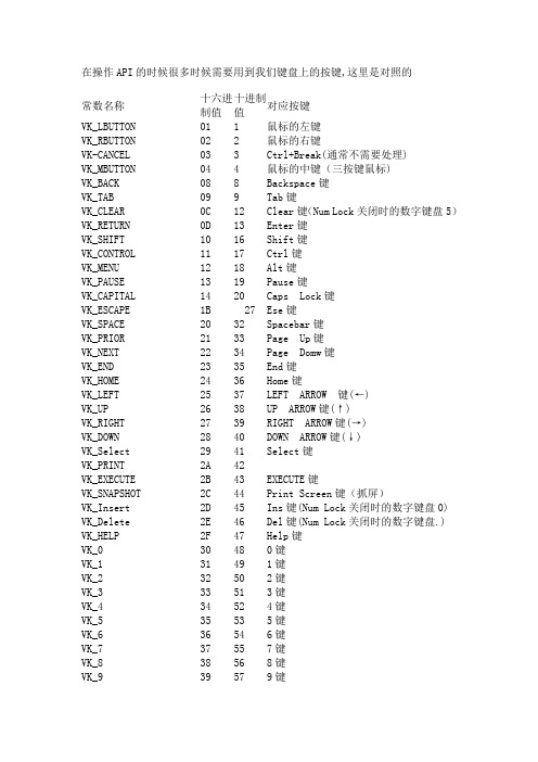
适用于:桌面应用程序
下表显示了符号常量的名称,十六进制值,鼠标或键盘等值的系统所使用的虚拟键码。按数字顺序列出的代码。
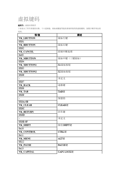
恒/值
描述
VK_LBUTTON
鼠标左键
0X01
VK_RBUTTON
鼠标右键
0X02
VK_CANCEL
控制中断处理
0x03
VK_MBUTTON
鼠标中键(三键鼠标)
0X04
VK_XBUTTON1
VK_MEDIA_PLAY_PAUSE
播放/暂停媒体键
0xB3
VK_LAUNCH_MAIL
启动邮件键
0xB4
VK_LAUNCH_MEDIA_SELECT
选择媒体键
0xB5
VK_LAUNCH_APP1
1键启动应用程序
0xB6
VK_LAUNCH_APP2
2键启动应用程序
0xB7
-
保留的
0XB8-B9
VK_OEM_1
0xBE
VK_OEM_2
用于其他字符,它可以通过键盘的不同而有所差异。
0xBF
对于美国标准键盘的“/?” 关键
VK_OEM_3
用于其他字符,它可以通过键盘的不同而有所差异。
0XC0
美国标准键盘,`〜“键
-
保留的
0xC1-D7
-
未分配
0xD8-DA
VK_OEM_4
用于其他字符,它可以通过键盘的不同而有所差异。
0xDB
美国标准键盘,“[{'键
VK_OEM_5
用于其他字符,它可以通过键盘的不同而有所差异。
0xDC
美国标准键盘的“\ |”键
VK_OEM_6
Time splitting for the Liouville equation in a random medium

with X fixed. The question is then how one should optimally choose the time step Θε = Tn+1 − Tn provided that the correlation length ε of the underlying Hamiltonian is known. It is a classical result [19] that the accuracy (in the strong L2 sense for instance) of the time splitting scheme is governed by Θε [A, Bε ] = Θε ABε − Bε A = O(Θε ε−3/2 ), where · is the L2 norm. The constraint Θε ε3/2 is necessary to fully resolve the solution of the Liouville equation, with an accuracy (in the strong L2 sense) of order Θε ε−3/2 . Instead of the classical time splitting scheme mentioned above, we could use the more accurate Strang time 2
∗
1
solution of the underlying wave equation in the high frequency limit [9, 16]. The parameter ε 1 measures the correlation length and time of the random medium relative to the overall propagation distance and time, respectively. It is small in the applications we have in mind. The strength of the potential is scaled in such a way that the above equation admits a physically interesting limit as ε → 0: see Section 2. We consider a time discretization of the above equation by a time splitting method [19]. Our analysis follows the method of study of the time splitting algorithm of a parabolic wave equation that we have used in [3]. Let us denote by 1 A = k · ∇x , Bε = − √ ∇x V ε t x , ε ε · ∇k
微专题 水溶液中的三大守恒和浓度大小比较(解析版)--高考化学微专题

水溶液中的三大守恒和浓度大小比较01考情分析02真题精研03规律·方法·技巧04经典变式练05核心知识精炼06基础测评07能力提升考情分析判断电解质溶液中粒子浓度的关系是高考常考题型,一般从单一溶液、混合溶液和不同溶液三个角度进行考查,其中反应过程中不同阶段粒子浓度关系的判断是近几年高考的热点和难点。
电离理论和水解理论是比较电解质溶液中粒子浓度大小关系的重要依据;电荷守恒、物料守恒和质子守恒是判断电解质溶液中粒子浓度等量关系的重要依据。
该类题目的解题关键是正确判断溶液中溶质成分及其量的关系,以及离子的电离程度和水解程度的大小。
真题精研1.(2024·湖南·高考真题)常温下K a HCOOH =1.8×10⁻⁴,向20mL0.10mol ⋅L -1NaOH 溶液中缓慢滴入相同浓度的HCOOH 溶液,混合溶液中某两种离子的浓度随加入HCOOH 溶液体积的变化关系如图所示,下列说法错误的是A.水的电离程度:M <NB.M 点:2c OH - =c Na + +c H +C.当V HCOOH =10mL 时,c OH - =c H + +2c HCOOH +c HCOO -D.N 点:c Na + >c HCOO - >c OH - >c H + >c HCOOH【答案】D【分析】结合起点和终点,向20mL0.10mol ⋅L -1NaOH 溶液中滴入相同浓度的HCOOH 溶液,发生浓度改变的微粒是Na +、OH -、H +和HCOO -;当V HCOOH =0mL ,溶液中存在Na +、H +和OH -,c OH - =c Na + =0.10mol ⋅L -1,随着加入HCOOH 溶液,c Na + 减少但不会降到0,当V HCOOH =20mL ,c Na + =0.05mol ⋅L -1,随着加入HCOOH 溶液,c OH - 会与HCOOH 反应而减少,当V HCOOH =20mL ,溶质为HCOONa ,n HCOONa =0.05mol ⋅L -1Kh =Kw Ka =10-141.8×10-4=c OH - c HCOOH c HCOO - =c OH - 2c HCOO - ⇒c OH -=10-10×0.05=1×10⁻⁵mol ⋅L -1c OH -很少,接近于0,则斜率为负的曲线代表c OH - ;当V HCOOH =0mL 时,0.10mol ⋅L -1NaOH 中c H + =10×10-13mol ⋅L -1,很小,随着加入HCOOH 溶液,溶质由NaOH 变为NaOH 和HCOONa 混物,最终为HCOONa ,c H + 增加的很少,而c HCOO - 增加的多,当V HCOOH =20mL ,溶质为HCOONa ,HCOO -少部分水解,n HCOO - <0.05mol ⋅L -1,斜率为正的曲线代表c HCOO - ,即经过M 点在下降的曲线表示的是OH -浓度的改变,经过M 点、N 点的在上升的曲线表示的是HCOO -浓度的改变。
小学语文-论语拼音版(五)
小学语文-论语拼音版(五)公(gōng)冶(yě)长(chng)篇(piān)第(dì)五(wǔ)子(zǐ)谓(wi)公(gōng)冶(yě)长(chng):可(kě)妻(qī)也(yě)。
虽(suī)在(zài)缧(li)绁(xi)之(zhī)中(zhōng),非(fēi)其(q)罪(zuì)也(yě)。
以(yǐ)其(q)子(zǐ)妻(qī)之(zhī)。
子(zǐ)谓(wi)南(nn)容(róng):邦(bāng)有(yǒu)道(dào),不(b)废(fi);邦(bāng)无(w)道(dào),免(miǎn)於(yū)刑(xng)戮(l)。
以(yǐ)其(q)兄(xiōng)之(zhī)子(zǐ)妻(qī)之(zhī)。
子(zǐ)谓(wi)子(zǐ)贱(jiàn):君(jūn)子(zǐ)哉(zāi)若(ruò)人(rn)!鲁(lǔ)无(w)君(jūn)子(zǐ)者(zhě),斯(sī)焉(yān)取(qǔ)斯(sī)?子(zǐ)贡(gòng)问(wn)曰(yuē):赐(cì)也(yě)何(h)如(r)?子(zǐ)曰(yuē):女(nǚ),器(qì)也(yě)。
曰(yuē):何(h)器(qì)也(yě)?曰(yuē):瑚(h)琏(liǎn)也(yě)。
或(huò)曰(yuē):雍(yōng)也(yě)仁(rn)而(r)不(b)佞(nìng)。
子(zǐ)曰(yuē):焉(yān)用(yòng)佞(nìng)?御(y)人(rn)以(yǐ)口(kǒu)给(gěi),屡(lǚ)憎(zēng)於(yū)人(rn)。
- 1、下载文档前请自行甄别文档内容的完整性,平台不提供额外的编辑、内容补充、找答案等附加服务。
- 2、"仅部分预览"的文档,不可在线预览部分如存在完整性等问题,可反馈申请退款(可完整预览的文档不适用该条件!)。
- 3、如文档侵犯您的权益,请联系客服反馈,我们会尽快为您处理(人工客服工作时间:9:00-18:30)。
广州大学毕业生就业政策知识测验
(附参考答案)
不定项选择题:(答案一个或多个,50题,2分/题,共100分)
1. 劳动合同期限三个月以上不满一年的,试用期不得超过个月;劳动合同期限一年以上不满三年的,试用期不得超过个月;三年以上固定期限和无固定期限的劳动合同,试用期不得超过个月。
A.一,三,六B.一,二,三 C.一,二,六 D.二,三,六
2. 关于试用期表述正确的是
A.同一用人单位与同一劳动者只能约定一次试用期。
B.以完成一定工作任务为期限的劳动合同或者劳动合同期限不满三个月的,不得约定试用期。
C.试用期不包含在劳动合同期限内。
D. 劳动合同仅约定试用期的,试用期不成立,该期限为劳动合同期限。
3. 劳动者在试用期的工资不得低于本单位相同岗位最低档工资或者劳动合同约定工资的百分之,并不得低于用人单位所在地的最低工资标准。
A.60% B.70% C.80% D.90%
4. 对“五险一金”理解正确的是
A.“五险”是指五种保险,包括养老保险、医疗保险、失业保险、工伤保险和生育保险,“一金”是指住房公积金。
B. “五险”均是由企业和个人共同缴纳的保费。
C. 单位录用职工的,应当自录用之日起30日内到住房公积金管理中心办理缴存登记。
D. 住房公积金全部由单位缴存。
5. 对《毕业生就业协议书》相关问题理解正确的是
A.《协议书》必须学生本人和用人单位及学校就业主管部门三方签署才有效。
B. 《协议书》只要学生本人和用人单位双方签署即有效。
C. 《协议书》每个学生只有一份。
D. 已经签约后又悔约的同学,在跟用人单位达成一致的解约意见前可先申请第二份《协议书》。
6. 对“生源地”理解正确的是
A. 生源地对大部分学生来说是指高考时候的户口所在地。
B. 对高考借考的同学来说,生源地就是指借考地。
C.生源地不同于籍贯和出生地。
D. 专插本的同学,其生源地是指就读专科前的常住户口所在地,如果是职中考进高职院校的,其生源地就应该以考入职中前户口所在地为准。
7. 学生张某,高考时户口所在地为广东梅州五华,且在五华参加高考,升大学时将户口迁至学校,在张某读大二的时候,父母由于工作调动原因将户口迁移到深圳,张某同学的生源地为。
A.梅州五华 B.学校户口所在地 C.深圳市 D.以上选项都不对
8.以下对与《报到证》相关问题表述正确的是
A. 学生遗失《报到证》不论多久均可申请补办。
B. 未取得毕业资格的毕业生一般没有报到证,待获得毕业证书后三个月内必须向学校就业中心申请办理《报到证》,超过三个月后申请的将不再受理。
C.在大学生就业在线网上申请了不就业并经审核后的升学的同学没有《报到证》。
D.按照民族生和定向生的相关规定,其《报到证》派遣回到生源地主管部门。
9.本科生李某,毕业前夕考研成功,顺利拿到了上海交大的研究生录取通知书,李某也在大学生就业在线申请了升学不参加就业,学校也审核通过了,李某就读研究生后不到2个月又找到了一个理想的单位,这时候李某能否重新申请派遣办理《报到证》?
A. 可以
B. 不可以
10. 对“改派”理解正确的是
A. 毕业生申请改派必须是在毕业后一年之内进行
B.暂缓就业一年后取消的也可以申请改派
C.申请改派的学生要提供的材料一般有原单位退函,新单位正式接受函,原《报到证》。
D. 已落实就业单位的毕业生不能随便申请办理改派。
11. 广州生源毕业生陈某,在毕业的时候没有落实就业单位,被派遣回生源地就业主管部门报到(即报到证抬头为广州市人力资源和社会保障局,报到部门是广州市高校毕业生就业指导中心),3个月后,陈某被广州市自来水公司正式录用,并签了三方协议,这时候陈某可去那个部门重新办理派遣手续?
A. 广州市高校毕业生就业指导中心B.学校就业指导中心
C. 一定要到广东省高校毕业生就业指导中心D. 不需要办理任何手续
12对暂缓就业理解正确的是
A.毕业当年超过6月10日后不能再申请办理暂缓就业。
B. 暂缓就业可以保留毕业生应届生的身份。
C.不能正常毕业的同学也可以申请办理暂缓就业。
D. 毕业前申请了升学的学生不能办理申请暂缓就业。