Hierarchical Latent Class Models and Statistical Foundation for Traditional Chinese Medicin

合集下载

latent-diffiusion预训练模型介绍

latent-diffiusion预训练模型介绍Latent Diffusion is a pre-training method that aims to improve the performance of various natural language processing (NLP) tasks. It leverages the principle of diffusion processes to learn better representations of text.The pre-training process of Latent Diffusion involves training a diffusion model on a large corpus of text. This diffusion model is trained to generate text in an autoregressive manner, where each token is generated conditioned on the previous tokens. The training objective is to minimize the reconstruction error of the generated text compared to the original text.During pre-training, the diffusion model learns to capture the underlying statistical structure of the text corpus, which enables it to generate coherent and meaningful text. The model learns to encode the semantics and syntax of the text into distributed representations, which can be used for downstream NLP tasks.The Latent Diffusion model can be fine-tuned on specific NLP tasks by adding task-specific layers on top of the pre-trained encoder. This allows the model to leverage the pre-trained representations for better performance on tasks like text classification, named entity recognition, machine translation, and more.Latent Diffusion has been shown to achieve state-of-the-art performance on various NLP benchmarks, demonstrating its effectiveness in learning high-quality text representations. Its pre-training process is unsupervised, making it scalable and adaptableto different domains and languages.In summary, Latent Diffusion is a pre-training method that utilizes diffusion processes to learn high-quality text representations. It can be fine-tuned for various NLP tasks and has demonstrated impressive performance on multiple benchmarks.。

AI术语

人工智能专业重要词汇表1、A开头的词汇：Artificial General Intelligence/AGI通用人工智能Artificial Intelligence/AI人工智能Association analysis关联分析Attention mechanism注意力机制Attribute conditional independence assumption属性条件独立性假设Attribute space属性空间Attribute value属性值Autoencoder自编码器Automatic speech recognition自动语音识别Automatic summarization自动摘要Average gradient平均梯度Average-Pooling平均池化Accumulated error backpropagation累积误差逆传播Activation Function激活函数Adaptive Resonance Theory/ART自适应谐振理论Addictive model加性学习Adversarial Networks对抗网络Affine Layer仿射层Affinity matrix亲和矩阵Agent代理/ 智能体Algorithm算法Alpha-beta pruningα-β剪枝Anomaly detection异常检测Approximation近似Area Under ROC Curve／AUC R oc 曲线下面积2、B开头的词汇Backpropagation Through Time通过时间的反向传播Backpropagation/BP反向传播Base learner基学习器Base learning algorithm基学习算法Batch Normalization/BN批量归一化Bayes decision rule贝叶斯判定准则Bayes Model Averaging／BMA贝叶斯模型平均Bayes optimal classifier贝叶斯最优分类器Bayesian decision theory贝叶斯决策论Bayesian network贝叶斯网络Between-class scatter matrix类间散度矩阵Bias偏置/ 偏差Bias-variance decomposition偏差-方差分解Bias-Variance Dilemma偏差–方差困境Bi-directional Long-Short Term Memory/Bi-LSTM双向长短期记忆Binary classification二分类Binomial test二项检验Bi-partition二分法Boltzmann machine玻尔兹曼机Bootstrap sampling自助采样法／可重复采样／有放回采样Bootstrapping自助法Break-Event Point／BEP平衡点3、C开头的词汇Calibration校准Cascade-Correlation级联相关Categorical attribute离散属性Class-conditional probability类条件概率Classification and regression tree/CART分类与回归树Classifier分类器Class-imbalance类别不平衡Closed -form闭式Cluster簇/类/集群Cluster analysis聚类分析Clustering聚类Clustering ensemble聚类集成Co-adapting共适应Coding matrix编码矩阵COLT国际学习理论会议Committee-based learning基于委员会的学习Competitive learning竞争型学习Component learner组件学习器Comprehensibility可解释性Computation Cost计算成本Computational Linguistics计算语言学Computer vision计算机视觉Concept drift概念漂移Concept Learning System /CLS概念学习系统Conditional entropy条件熵Conditional mutual information条件互信息Conditional Probability Table／CPT条件概率表Conditional random field/CRF条件随机场Conditional risk条件风险Confidence置信度Confusion matrix混淆矩阵Connection weight连接权Connectionism连结主义Consistency一致性／相合性Contingency table列联表Continuous attribute连续属性Convergence收敛Conversational agent会话智能体Convex quadratic programming凸二次规划Convexity凸性Convolutional neural network/CNN卷积神经网络Co-occurrence同现Correlation coefficient相关系数Cosine similarity余弦相似度Cost curve成本曲线Cost Function成本函数Cost matrix成本矩阵Cost-sensitive成本敏感Cross entropy交叉熵Cross validation交叉验证Crowdsourcing众包Curse of dimensionality维数灾难Cut point截断点Cutting plane algorithm割平面法4、D开头的词汇Data mining数据挖掘Data set数据集Decision Boundary决策边界Decision stump决策树桩Decision tree决策树／判定树Deduction演绎Deep Belief Network深度信念网络Deep Convolutional Generative Adversarial Network/DCGAN深度卷积生成对抗网络Deep learning深度学习Deep neural network/DNN深度神经网络Deep Q-Learning深度Q 学习Deep Q-Network深度Q 网络Density estimation密度估计Density-based clustering密度聚类Differentiable neural computer可微分神经计算机Dimensionality reduction algorithm降维算法Directed edge有向边Disagreement measure不合度量Discriminative model判别模型Discriminator判别器Distance measure距离度量Distance metric learning距离度量学习Distribution分布Divergence散度Diversity measure多样性度量／差异性度量Domain adaption领域自适应Downsampling下采样D-separation （Directed separation）有向分离Dual problem对偶问题Dummy node哑结点Dynamic Fusion动态融合Dynamic programming动态规划5、E开头的词汇Eigenvalue decomposition特征值分解Embedding嵌入Emotional analysis情绪分析Empirical conditional entropy经验条件熵Empirical entropy经验熵Empirical error经验误差Empirical risk经验风险End-to-End端到端Energy-based model基于能量的模型Ensemble learning集成学习Ensemble pruning集成修剪Error Correcting Output Codes／ECOC纠错输出码Error rate错误率Error-ambiguity decomposition误差-分歧分解Euclidean distance欧氏距离Evolutionary computation演化计算Expectation-Maximization期望最大化Expected loss期望损失Exploding Gradient Problem梯度爆炸问题Exponential loss function指数损失函数Extreme Learning Machine/ELM超限学习机6、F开头的词汇Factorization因子分解False negative假负类False positive假正类False Positive Rate/FPR假正例率Feature engineering特征工程Feature selection特征选择Feature vector特征向量Featured Learning特征学习Feedforward Neural Networks/FNN前馈神经网络Fine-tuning微调Flipping output翻转法Fluctuation震荡Forward stagewise algorithm前向分步算法Frequentist频率主义学派Full-rank matrix满秩矩阵Functional neuron功能神经元7、G开头的词汇Gain ratio增益率Game theory博弈论Gaussian kernel function高斯核函数Gaussian Mixture Model高斯混合模型General Problem Solving通用问题求解Generalization泛化Generalization error泛化误差Generalization error bound泛化误差上界Generalized Lagrange function广义拉格朗日函数Generalized linear model广义线性模型Generalized Rayleigh quotient广义瑞利商Generative Adversarial Networks/GAN生成对抗网络Generative Model生成模型Generator生成器Genetic Algorithm/GA遗传算法Gibbs sampling吉布斯采样Gini index基尼指数Global minimum全局最小Global Optimization全局优化Gradient boosting梯度提升Gradient Descent梯度下降Graph theory图论Ground-truth真相／真实8、H开头的词汇Hard margin硬间隔Hard voting硬投票Harmonic mean调和平均Hesse matrix海塞矩阵Hidden dynamic model隐动态模型Hidden layer隐藏层Hidden Markov Model/HMM隐马尔可夫模型Hierarchical clustering层次聚类Hilbert space希尔伯特空间Hinge loss function合页损失函数Hold-out留出法Homogeneous同质Hybrid computing混合计算Hyperparameter超参数Hypothesis假设Hypothesis test假设验证9、I开头的词汇ICML国际机器学习会议Improved iterative scaling/IIS改进的迭代尺度法Incremental learning增量学习Independent and identically distributed/i.i.d.独立同分布Independent Component Analysis/ICA独立成分分析Indicator function指示函数Individual learner个体学习器Induction归纳Inductive bias归纳偏好Inductive learning归纳学习Inductive Logic Programming／ILP归纳逻辑程序设计Information entropy信息熵Information gain信息增益Input layer输入层Insensitive loss不敏感损失Inter-cluster similarity簇间相似度International Conference for Machine Learning/ICML国际机器学习大会Intra-cluster similarity簇内相似度Intrinsic value固有值Isometric Mapping/Isomap等度量映射Isotonic regression等分回归Iterative Dichotomiser迭代二分器10、K开头的词汇Kernel method核方法Kernel trick核技巧Kernelized Linear Discriminant Analysis／KLDA核线性判别分析K-fold cross validation k 折交叉验证／k 倍交叉验证K-Means Clustering K –均值聚类K-Nearest Neighbours Algorithm/KNN K近邻算法Knowledge base知识库Knowledge Representation知识表征11、L开头的词汇Label space标记空间Lagrange duality拉格朗日对偶性Lagrange multiplier拉格朗日乘子Laplace smoothing拉普拉斯平滑Laplacian correction拉普拉斯修正Latent Dirichlet Allocation隐狄利克雷分布Latent semantic analysis潜在语义分析Latent variable隐变量Lazy learning懒惰学习Learner学习器Learning by analogy类比学习Learning rate学习率Learning Vector Quantization/LVQ学习向量量化Least squares regression tree最小二乘回归树Leave-One-Out/LOO留一法linear chain conditional random field线性链条件随机场Linear Discriminant Analysis／LDA线性判别分析Linear model线性模型Linear Regression线性回归Link function联系函数Local Markov property局部马尔可夫性Local minimum局部最小Log likelihood对数似然Log odds／logit对数几率Logistic Regression Logistic 回归Log-likelihood对数似然Log-linear regression对数线性回归Long-Short Term Memory/LSTM长短期记忆Loss function损失函数12、M开头的词汇Machine translation/MT机器翻译Macron-P宏查准率Macron-R宏查全率Majority voting绝对多数投票法Manifold assumption流形假设Manifold learning流形学习Margin theory间隔理论Marginal distribution边际分布Marginal independence边际独立性Marginalization边际化Markov Chain Monte Carlo/MCMC马尔可夫链蒙特卡罗方法Markov Random Field马尔可夫随机场Maximal clique最大团Maximum Likelihood Estimation/MLE极大似然估计／极大似然法Maximum margin最大间隔Maximum weighted spanning tree最大带权生成树Max-Pooling最大池化Mean squared error均方误差Meta-learner元学习器Metric learning度量学习Micro-P微查准率Micro-R微查全率Minimal Description Length/MDL最小描述长度Minimax game极小极大博弈Misclassification cost误分类成本Mixture of experts混合专家Momentum动量Moral graph道德图／端正图Multi-class classification多分类Multi-document summarization多文档摘要Multi-layer feedforward neural networks多层前馈神经网络Multilayer Perceptron/MLP多层感知器Multimodal learning多模态学习Multiple Dimensional Scaling多维缩放Multiple linear regression多元线性回归Multi-response Linear Regression ／MLR多响应线性回归Mutual information互信息13、N开头的词汇Naive bayes朴素贝叶斯Naive Bayes Classifier朴素贝叶斯分类器Named entity recognition命名实体识别Nash equilibrium纳什均衡Natural language generation/NLG自然语言生成Natural language processing自然语言处理Negative class负类Negative correlation负相关法Negative Log Likelihood负对数似然Neighbourhood Component Analysis/NCA近邻成分分析Neural Machine Translation神经机器翻译Neural Turing Machine神经图灵机Newton method牛顿法NIPS国际神经信息处理系统会议No Free Lunch Theorem／NFL没有免费的午餐定理Noise-contrastive estimation噪音对比估计Nominal attribute列名属性Non-convex optimization非凸优化Nonlinear model非线性模型Non-metric distance非度量距离Non-negative matrix factorization非负矩阵分解Non-ordinal attribute无序属性Non-Saturating Game非饱和博弈Norm范数Normalization归一化Nuclear norm核范数Numerical attribute数值属性14、O开头的词汇Objective function目标函数Oblique decision tree斜决策树Occam’s razor奥卡姆剃刀Odds几率Off-Policy离策略One shot learning一次性学习One-Dependent Estimator／ODE独依赖估计On-Policy在策略Ordinal attribute有序属性Out-of-bag estimate包外估计Output layer输出层Output smearing输出调制法Overfitting过拟合／过配Oversampling过采样15、P开头的词汇Paired t-test成对t 检验Pairwise成对型Pairwise Markov property成对马尔可夫性Parameter参数Parameter estimation参数估计Parameter tuning调参Parse tree解析树Particle Swarm Optimization/PSO粒子群优化算法Part-of-speech tagging词性标注Perceptron感知机Performance measure性能度量Plug and Play Generative Network即插即用生成网络Plurality voting相对多数投票法Polarity detection极性检测Polynomial kernel function多项式核函数Pooling池化Positive class正类Positive definite matrix正定矩阵Post-hoc test后续检验Post-pruning后剪枝potential function势函数Precision查准率／准确率Prepruning预剪枝Principal component analysis/PCA主成分分析Principle of multiple explanations多释原则Prior先验Probability Graphical Model概率图模型Proximal Gradient Descent/PGD近端梯度下降Pruning剪枝Pseudo-label伪标记16、Q开头的词汇Quantized Neural Network量子化神经网络Quantum computer量子计算机Quantum Computing量子计算Quasi Newton method拟牛顿法17、R开头的词汇Radial Basis Function／RBF径向基函数Random Forest Algorithm随机森林算法Random walk随机漫步Recall查全率／召回率Receiver Operating Characteristic/ROC受试者工作特征Rectified Linear Unit/ReLU线性修正单元Recurrent Neural Network循环神经网络Recursive neural network递归神经网络Reference model参考模型Regression回归Regularization正则化Reinforcement learning/RL强化学习Representation learning表征学习Representer theorem表示定理reproducing kernel Hilbert space/RKHS再生核希尔伯特空间Re-sampling重采样法Rescaling再缩放Residual Mapping残差映射Residual Network残差网络Restricted Boltzmann Machine/RBM受限玻尔兹曼机Restricted Isometry Property/RIP限定等距性Re-weighting重赋权法Robustness稳健性/鲁棒性Root node根结点Rule Engine规则引擎Rule learning规则学习18、S开头的词汇Saddle point鞍点Sample space样本空间Sampling采样Score function评分函数Self-Driving自动驾驶Self-Organizing Map／SOM自组织映射Semi-naive Bayes classifiers半朴素贝叶斯分类器Semi-Supervised Learning半监督学习semi-Supervised Support Vector Machine半监督支持向量机Sentiment analysis情感分析Separating hyperplane分离超平面Sigmoid function Sigmoid 函数Similarity measure相似度度量Simulated annealing模拟退火Simultaneous localization and mapping同步定位与地图构建Singular Value Decomposition奇异值分解Slack variables松弛变量Smoothing平滑Soft margin软间隔Soft margin maximization软间隔最大化Soft voting软投票Sparse representation稀疏表征Sparsity稀疏性Specialization特化Spectral Clustering谱聚类Speech Recognition语音识别Splitting variable切分变量Squashing function挤压函数Stability-plasticity dilemma可塑性-稳定性困境Statistical learning统计学习Status feature function状态特征函Stochastic gradient descent随机梯度下降Stratified sampling分层采样Structural risk结构风险Structural risk minimization/SRM结构风险最小化Subspace子空间Supervised learning监督学习／有导师学习support vector expansion支持向量展式Support Vector Machine/SVM支持向量机Surrogat loss替代损失Surrogate function替代函数Symbolic learning符号学习Symbolism符号主义Synset同义词集19、T开头的词汇T-Distribution Stochastic Neighbour Embedding/t-SNE T–分布随机近邻嵌入Tensor张量Tensor Processing Units/TPU张量处理单元The least square method最小二乘法Threshold阈值Threshold logic unit阈值逻辑单元Threshold-moving阈值移动Time Step时间步骤Tokenization标记化Training error训练误差Training instance训练示例／训练例Transductive learning直推学习Transfer learning迁移学习Treebank树库Tria-by-error试错法True negative真负类True positive真正类True Positive Rate/TPR真正例率Turing Machine图灵机Twice-learning二次学习20、U开头的词汇Underfitting欠拟合／欠配Undersampling欠采样Understandability可理解性Unequal cost非均等代价Unit-step function单位阶跃函数Univariate decision tree单变量决策树Unsupervised learning无监督学习／无导师学习Unsupervised layer-wise training无监督逐层训练Upsampling上采样21、V开头的词汇Vanishing Gradient Problem梯度消失问题Variational inference变分推断VC Theory VC维理论Version space版本空间Viterbi algorithm维特比算法Von Neumann architecture冯·诺伊曼架构22、W开头的词汇Wasserstein GAN/WGAN Wasserstein生成对抗网络Weak learner弱学习器Weight权重Weight sharing权共享Weighted voting加权投票法Within-class scatter matrix类内散度矩阵Word embedding词嵌入Word sense disambiguation词义消歧23、Z开头的词汇Zero-data learning零数据学习Zero-shot learning零次学习。

[电脑基础知识]spss多水平模型简介

Harvey Goldstein, UK, University of London, Institute of Education
《Multilevel Models in Educational and Social Research》1987
Anthony Bryk, University of Chicago Stephen Raudenbush, Michigan State University , Department of Educational Psychology
进一步，如数据具三个水平的层次结构，如医院、医生和患者三个水平，则将有两个这样的相关系数，即反映医院之间方差比例的医院内相关，反映医生之间方差比例的医生内相关。
随机系数模型
(Random Coefficient Model)
随机系数模型是指协变量的系数估计不是固定的而是随机的，即协变量对反应变量的效应在不同的水平 2 单位间是不同的。
Va(u r0j)
2 u0
对患者水平残差的假定与传统模型一致
E(e0ij) 0， Va(er0ij)e20
水平 1 上的残差与水平 2 上的残差相互独立
Co(uv0j,e0ij)0
y i j 0 1 x i j u 0 j e 0 i j
反应变量可表达为固定部分 01xij 与随机部分 u0j e0ij 之和。模型具有两个残差项，
斜率估计，表明协变量 x ij 对反应变量的效应
在各个医院间是不同的。
0 j 的假定及其含义与方差成份模型一
致。现 1 j 为随机变量，假定：
E(1j )1 Va(r1j)u21
1 j 表示第 j 个医院的 y 随 x 变化的斜

HierarchicalModels：分层模型

transformation from simpler ones!
12
Derive Equation
• Now, light source at origin
y
light source
x
y -yl = yp
a point on object
(x, y, z)
x
(xp, yp, zp) xp
shadow
21
Hierarchical Models
• Many graphical objects are structured
• Exploit structure for
– Efficient rendering – Example: bounding
boxes (later in course) – Concise specification of
24
Sample Instance Transformation
glMatrixMode(GL_MODELVIEW); glLoadIdentity(); glTranslatef(...); glRotatef(...); glScalef(...); gluCylinder(...);
25
Display Lists
• Sharing display commands • Display lists are stored on the GPU • May contain drawing commands and transfns. • Initialization:
GLuint torus = glGenLists(1); glNewList(torus, GL_COMPILE);
glTranslatef(xl, yl, zl); /* translate back */

Structural EM for Hierarchical Latent Class Models

Structural EM for Hierarchical Latent ClassModelsTechnical Report HKUST-CS03-06Nevin L.ZhangDepartment of Computer ScienceHong Kong University of Science&Technology,Chinalzhang@t.hkAbstractHierarchical latent class(HLC)models are tree-structured Bayesian networks where leaf nodes are observed while internal nodes are not.This paper is concerned with the problem of learning HLC models from data.We apply the idea of structural EM to a hill-climbing algorithm for this task described in an accompanying paper(Zhang et al.2003)and show empirically that the improved algorithm can learn HLC models that are large enough to be of practical interest.1INTRODUCTIONHierarchical latent class(HLC)models(Zhang2002)are tree-structured Bayesian networks(BNs)where leaf nodes are observed while internal nodes are not.They generalize latent class(LC)models(Lazarsfeld and Henry 1968)and were identiﬁed as a potentially useful class of Bayesian networks by Pearl(1988).This paper is con-cerned with the problem of learning HLC models from data.The problem is interesting for three reasons.First, HLC models represent complex dependencies among observed variables and yet are computationally simple to work with.Second,the endeavor of learning HLC models can reveal latent causal structures.Researchers have already been inferring latent causal structures from observed data.One example is the reconstruction of phylo-genetic trees(Durbin et al.1998),which can be viewed as special HLC models.Third,HLC models alleviate disadvantages of LC models as models for cluster analysis.This in fact was the motivation for the introduction of HLC models.When learning BNs with latent variables,one needs to determine not only model structures,i.e.connections among variables,but also cardinalities of latent variables,i.e.the numbers of values they can take.Although not using the terminology of HLC models,Connolly(1993)proposed theﬁrst,somewhat ad hoc,algorithm for learning HLC models.A more principled algorithm was proposed by Zhang(2002).This algorithm hill-climbs in the space HLC model structures.For each model structure,a separate hill-climbing routine is called to optimize the cardinalities of its latent variables.Hence we refer to the algorithm as the double hill-climbing(DHC)algorithm. Another hill-climbing algorithm is described in Zhang et al.(2003).This algorithm optimizes model structures and cardinalities of latent variables at the same time and hence does not need a separate routine for the latter. Consequently,it is called the single hill-climbing(SHC)algorithm.SHC is signiﬁcantly more efﬁcient than DHC. In this paper,a followup of Zhang et al.(2003),we further speed up SHC by applying the idea of structural EM (Friedman1997).Structural EM was introduced for the task of learning Bayesian networks from data with missing values.It assumes that there is aﬁxed and known set of variables.One knows not only what the variables are,but also what possible values each variable can take.All candidate models encountered during hill-climbing involve exactly those variables.This assumption is not true when learning HLC models.We do not know what the latent variables are.We do not even know how many latent variables there should be and how many values each latent variable should take.This is the main technical issue that we need to address.We start in the next section with a brief review the necessary background.In Section3,we present our method for applying the idea of structural EM to SHC.Empirical results are reported in Section4and conclusions provided in Section5.2HLC MODELS AND THE SHC ALGORITHMThis section gives a brief review of HLC models and the SHC algorithm.Readers are referred to Zhang(2002) and Zhang et al.(2003)for details.2.1HLC MODELSA hierarchical latent class(HLC)model is a Bayesian network where(1)the network structure is a rooted tree and(2)the variables at the leaf nodes are observed and all the other variables are not.An example HLC model is shown in Figure1(on the left).In this paper,we use the terms“node”and“variable”interchangeably.The observed variables are referred to as manifest variables and all the other variables as latent variables.A latent class(LC)model is an HLC model where there is only one latent node.We usually write an HLC model as a pair,where is the collection of parameters.Theﬁrst component consists of the model structure and cardinalities of the variables.We will sometimes refer to also as an HLC model.When it is necessary to distinguish between and the pair,we call an unparameterized HLC model and the pair a parameterized HLC model.Two parameterized HLC models and are marginally equivalent if they share the same manifest variables,,...,and(1)X2Y5Y6Y7X3X1Y4Y1Y2Y3Figure1:An example HLC model and the corresponding unrooted HLC model.The’s are latent variables and the’s are manifest variables.An unparameterized HLC models includes another if for any parameterization of,there exists param-eterization of such that and are marginally equivalent,i.e.if can represent any distributions over the manifest variables that can.If includes and vice versa,we say that and are marginally equivalent.Marginally equivalent(parameterized or unparameterized)models are equivalent if they have the same number of independent parameters.One cannot distinguish between equivalent models using penalized likelihood scores(Green1998).Let be the root of an HLC model.Suppose is a child of and it is a latent node.Deﬁne another HLC model by reversing the arrow.In,is the root.The operation is hence called root walking; the root has walked from to.Root walking leads to equivalent models(Zhang2002).This implies that it is impossible to determine edge orientation from data.We can learn only unrooted HLC models,which are HLC models with all directions on the edges dropped.Figure1also shows an example unrooted HLC model. An unrooted HLC model represents a class of HLC models.Members of the class are obtained by rooting the model at various nodes and by directing the edges away from the root.Semantically it is a Markov randomﬁeld on an undirected tree.The leaf nodes are observed while the interior nodes are latent.The concepts of marginal equivalence and equivalence can be deﬁned for unrooted HLC models in the same way as for rooted models. From now on when we speak of HLC models we always mean unrooted HLC models unless it is explicitly stated otherwise.Let stand for the cardinality of a variable.For a latent variable in an HLC model,enumerate its neighbors as,,...,.An HLC model is regular if for any latent variable,(3)Note that this deﬁnition applies to parameterized as well as to unparameterized models.Given an irregular parameterized model,there exists,a regular model that is marginally equivalent to and has fewer independent parameters(Zhang2002).Such a regular model can be obtained from by deleting,one by one,nodes that violate Condition(3)and reducing the cardinality of each node that violates Condition(2)to the quantity on the right hand side.The second step needs to be repeated until cardinalities of latent variables can no longer be reduced.We refer to the process as regularization.It is evident that if penalized likelihood is used for model selection,the regularized model is always preferred over itself.2.2THE SHC ALGORITHMAssume that there is a collection of i.i.d samples on a number of manifest variables generated by an unknown regular HLC model.SHC aims at reconstructing the regular unrooted HLC models that corresponds to the gener-ative model.It does so by hill-climbing in the space of all unrooted regular HLC models for the given manifest variables.For this paper,we assume that the BIC score is used to guide the search.The BIC score of a model isX Y6Y5Y4XX1m1m2X1m3Y3Y2Y1XY4Y5Y6Y3Y2Y1Y6Y5Y4Y3Y2Y1Figure2:Illustration of Node Introduction and Node Relocation.The overall strategy of SHC is similar to that of greedy equivalence search(GES),an algorithm for learning Bayesian network structures in the case when all variables are observed(Meek1997).It begins with the simplest HLC model and works in two phases.In Phase I,SHC expands models by introducing new latent nodes and additional states for existing nodes.The aim is to improve the likelihood term of the BIC score.In Phase II,SHC retracts models by deleting latent nodes or states of latent nodes.The aim is to reduce the penalty term of the BIC score,while keeping the likelihood term more or less the same.If model quality is improved in Phase II,SHC goes back to Phase I and the process repeats itself.Search operators:SHC hill-climbs usingﬁve search operators,namely State Introduction,Node Introduction, Node Relocation,State Deletion,and Node Deletion.Theﬁrst three operators are used in Phase I and the rest are used in Phase II.Given an HLC model and a latent variable in the model,State Introduction(SI)creates a new model by adding a state to the state space of the variable.The opposite of SI is State Deletion(SD),which creates a new model by deleting a state from the state space of a variable.Node Introduction(NI)involves one latent node in an HLC model and two of its neighbors.It creates a new model by introducing a new latent node to mediate and the two neighbors.The new node has the same cardinality as.Consider the HLC model in Figure2.Applying the NI operator to the latent Node and its neighbors and results in the model.The new node has the same state space as.The opposite of NIis Node Deletion(ND).It involves two neighboring latent nodes and.It creates a new model by deleting and making all neighbors of other than neighbors of.Called Node Relocation(NR),the next operator re-arranges connections among existing nodes.It involves a latent node and two of its neighbors and,where must also be a latent node.It creates a new model by relocating to,i.e.removing the link between and and adding a link between and.Consider the HLC model in Figure2.Relocating from to results in model.There is a variant to NR that we call Accommodating Node Relocation(ANR).It is the same as NR except that,after relocating a node,it adds one state to its new neighbor.All of theﬁve operators might lead to the violation of the regularity constraints.We therefore follow each operator immediately with a regularization step.Model selection:At each step of search,SHC generates a number of candidate models by applying the search operators to the current model.It then selects one of the candidate models and moves to the next step.As argued in Zhang et al.(2003),the strategy of simply choosing the one with the highest score does not work.Let be the current model and be a candidate model.Deﬁne the unit improvement of over given to beModel selection in Phase II is straightforward and is based on model score.Pseudo code:We now give the pseudo code for the SHC algorithm.The input to the algorithm is a data set on a list of manifest variables.Records in do not necessarily contain values for all the manifest variables.The output is an unrooted HLC model.Model parameters are optimized using the EM algorithm.Given a model, the collections of candidate models the search operators produce will be respectively denoted by,, ,,,and.Let be the LC model with a binary latent node.Repeat until termination:.If,return.Else..If,return.Else.Repeat until termination:Remove from and all modelss.t.,If there is s.t.and continue.Find inthat maximizes.If,return m.Else.Repeat until termination:Find the model inthat maximizes.If,return m.Else.3THE HEURISTIC SHC ALGORITHMAt each step of search,SHC generates a set of candidate models,evaluates each of them,and selects the best one.Before a model can be evaluated,its parameters must be optimized.Due to the presence of latent variables, parameters are optimized using the EM algorithm.EM is known to be computationally expensive.SHC runs EM on each candidate model and is hence inefﬁcient(Zhang et al.2003).The same problem confronts hill-climbing algorithms for learning general Bayesian networks from data with missing values.There,structural EM was proposed to reduce the number of calls to EM(Friedman1997).The idea is to complete the data,orﬁll in the missing values,using the current model and then evaluate the candidate models based on the completed data.Parameter optimization based on the completed data does not require EM at all.EM is called only once at the end of each iteration to optimize the parameters of the best candidate model.In this section,we apply the idea of structural EM to SHC.The main technical issue that we need to address is that the variables in the candidate models can differ slightly different from those in the current model.Hence there might be a slight mismatch between the completed data and the candidate models.In a candidate model generated by the NI operator,for instance,there is one new variable that does not appear in the current model.The completed data contain no values for the new variable.How should we evaluate a candidate model based on a slightly mismatched data set?The answer depends how the candidate model is generated,i.e.by which operator.We divide all the candidate models into several groups, with one group for each operator.Models in a group are compared with each other based on the completed data and the best one is selected.Thereafter a second model selection process is invoked to choose one from the best models of the groups.This second process is the same as the model selection process in SHC,except that there is only one candidate model for each operator.In this phase,parameters of models are optimized using EM.3.1MODEL SELECTION IN PHASE IIn the next3subsections,we discuss how to select among candidate models generated by each of the search operators used in Phase I.Here are some notations that we will use.We use to denote the current model andto denote the ML estimate of the parameters of based on the data set.The estimate was computed using EM at the end of the previous step.Let be the joint probability represented by the parameterized model.Completing the data set using the parameterized model,we get a data set that contain values for all variables in.Denote the completed data set by.Let the set of variables in.induces an empirical distribution over,which we denote by.In the following,we will need to refer to the quantities of and ,where and are subsets of variables.Such quantities are computed from the parameterized model and the original data set.They are not obtained from the completed data set.In fact,we never explicitly compute the completed data set.It is introduced only for conceptual clarity.3.2SELECTING AMONG MODELS GENERATED BY NIConsider a candidate model in.Suppose it is obtained from by introducing a latent variable to mediate the interactions between a node and two of its neighbors and.Deﬁne(5)This is the criterion that we use to select among models in;We select the one that maximizes the quantity.The criterion is intuitively appealing.Consider the term on the numerator of the expression on the right hand side of(5).Except for a constant factor of2,it is the G-squared statistic,based on,for testing the hypothesis that and are conditionally independent given.The larger the term,the further away and are from being independent given,and the more improvement in model quality the NI operation would bring about.So selecting the candidate model in that maximizes amounts to choosing the way to apply NI operator that would result in the largest increase in model quality per complexity unit.The criterion not only is intuitively appealing,but also follows from the cost-effectiveness principle.We explain why in the rest of this subsection.The cost-effectiveness principle states that we should choose the model in that maximizes:where stands for the set of parents of in.The challenge is to compute term.Let be the ML estimate of the parameters of based on .Use to denote the joint probability represented by parameterized model.Consider a variable in that is not,,or.The parents of in are the same as those in.Moreover,the variable and it parents are observed in the data set.Hence we have Consequently, is given bywhere One can estimate the conditional probability distribu-tions,,and from.But this requires running EM because does not contain values for.Not wanting to run EM,we seek an approximation for the second term on the right hand side of the above equation.We choose to approximate it with the maximum value possible,i.e.. This leads to the following approximation of(9) Let the set of variables in.It is the same as the set of variables in except for.Let be the ML estimate of parameters of based e to denote the joint probability distributions represented by the parameterized model.For technical convenience,root at node and at node.Then is given byTo obtain,one needs to run EM.Not wanting to run EM,we approximate it using the same joint probability in the parameterized model.The above two approximations lead to the following approximation of:(10) Substituting this for in(9),simplifying the resulting expression,and removing terms that does not depend on,we obtain the right hand side of(7).3.4SELECTING AMONG MODELS GENERATED BY NR AND ANRConsider a candidate model in.Suppose it is obtained from by relocating a neighbor of a node to another neighbor of.For technical convenience,assume is rooted at.Thenis given by(11)Among all models in,we choose the one for which this difference is the largest.Consider a candidate model in that is obtained from byﬁrst relocating a neighbor of a node to another neighbor of and then increasing the cardinality of by one.Let be the same as except that the cardinality of is not increased.Let be the data set obtained from by deleting values of.We view ANR as a combination of NR and SI and hence evaluate candidate models in using the following criterion:(12) where is computed using(11)and the second term is approximated using a formula similar to(8).It is possible that might be the same as.In that case,we set the denominator to a small number(0.01in experiments reported in this paper).3.5MODEL SELECTION IN PHASE IIConsider a candidate model in.Suppose it is obtained from by deleting a latent node.Suppose the neighbors of in are,,...,and suppose the’s are made neighbors of.For technical convenience, assume is rooted at.Then is given byM1M3M5Figure3:Test Models:Manifest nodes are labelled with their names.All manifest variables tent nodes are labelled with their cardinalities.3.7LOCAL EMBy applying the idea of structural EM,we have substantially reduced the number of calls to EM.Nonetheless westill need to run EM on a number of models at each step of search.Within the top-scheme,we need to run EM on models for each of the operators except for SD.For SD,we need to run EM on models,where is thenumber of latent nodes in the current model.To achieve further speedup,we replace all those calls to EM withcalls to a more efﬁcient procedure that we refer to as local EM.Parameters of the current model were estimated at the end of the previous search step.Each candidatemodel generated at the current search step differs from only slightly.The idea of local EM is to optimize the conditional probability distributions(CPDs)of only a few variables in,while keeping those of other variablesthe same as in.If is obtained from by adding a state to or deleting a state from a variable,then only theCPD’s that involve are optimized.If is obtained from by introducing a latent node to separate a node from two of its neighbors,then only the CPD’s that involve and are optimized.If is obtained from by relocating a node from to,then only the CPD’s that involve and are optimized.Finally,if isobtained from by deleting a node and making all neighbors except for one,which we denote by,neighbors of,then only the CPD’s that involve are optimized.Obviously,model parameters provided by local EM deviate from those provided by EM.To avoid accumulationof deviations,we run EM once at the end of each search step on the model that is selected as the best at that step. 4EMPIRICAL RESULTSThis section reports experiments designed to determine whether the heuristic SHC(HSHC)algorithm can learnmodels of good quality and how efﬁcient it is.In all the experiments,EM and local EM were conﬁgured asfollows.To estimate all/some of the parameters for a given unparameterized/partially parameterized model,we ﬁrst randomly generated64sets of parameters for the model,resulting in64initial fully parameterized models1. One EM/local EM iteration was run on all models and afterwards the worst32models were discarded.Then two EM/local EM iterations were run on the remaining32models and afterwards the worst16models were discarded. This process was continued until there was only one model.On this model,EM/local EM were terminated either if the increase in loglikelihood fell below0.01or the total number of iterations exceeded500.Our experiments were based on synthetic data.We used5generative models that consist of6,9,12,15,and18manifest variables respectively.The total numbers of variables in the models are9,13,19,23,and28respectively.Three of the models are shown in Figure3.Parameters were randomly generated except that we ensured that each0.010.1810121416182022242628E m p i r i c a l K L Problem Size shc hshc3hshc2hshc1Figure 4:Empirical KL divergences of learned models from the generative models.223a b c 2e 3d 23g h i 3j k l 23m n o 2p q rFigure 5:The unrooted HLC model reconstructed by HSHC3for test model M5.conditional distribution has a component with mass larger than 0.8.We also ensured that,in every conditional probability table,that the large components of different rows are not all at the same column.A data set of 10,000records were sampled for each model.We then ran SHC and HSHC to reconstruct the generative models from the data sets.HSHC was tested on all the 5data sets,while SHC was tested on only 3,i.e.those sampled from the 3simplest generative models.For HSHC,the top-scheme was used,with running from 1to 3.So we in fact tested three versions of the algorithm.We will refer to them using HSHC1,HSHC2,and HSHC3.The algorithms were implemented in Java and all experiments were run on a Pentium 4PC with a clock rate of 2.26GHz.To measure the quality of the learned models,a testing set of 5,000records were sampled from each generative model.The log score of each learned model and the log score of the corresponding original model were computed.Letbe the number records in in general.Note that as goes to inﬁnity the average log score difference tends to ,the KL divergence of the probability distribution of manifest variables in the learned model from that of manifest variables in the original model.We hence refer to it as empirical KL divergence .It is a good measure of the quality of the learned model.The emprical divergences between the learned models and the original models are shown in 4.We see that some of the models reconstructed by HSHC1are of poor quality in two of the ﬁve cases.However,all the models reconstructed by HSHC2and HSHC3match the generative models extremely well in terms of distribution over the manifest variables.The structures of these models are either identical or very similar to the structures of the generative models.The structure of the model produced by HSHC3for M5is shown in Figure 5.It is very close to the structure of M5.Time statistics are shown in Figure (6).We see that HSHC is much more efﬁciently than SHC and it scales up fairly well.HLC models were motivated by an application in traditional Chinese medicine (Zhang 2002).HSHC is efﬁcient enough for us to induce interesting models for that application.5CONCLUSIONSIt is interesting to learn HLC models because,as models for cluster analysis,they relax the often untrue conditional independence assumption of LC models and hence suit more applications.They also facilitate the discovery of latent causal structures and the induction of probabilistic models that capture complex correlations and yet have low inferential complexity.050000100000150000200000250000300000810121416182022242628T i m e (s e c o n d s )Problem Size shc hshc3hshc2hshc1Figure 6:Time statistics.In this paper,we apply the idea of structural EM to a previous algorithm for learning HLC models.Called HSHC,the improved algorithm has been empirically shown to be capable of inducing HLC models that are large enough to be of practical interest.AcknowledgementsI thank Tomas Kocka,Finn V .Jensen,and Gytis Karciauskas for valuable discussions.Research was partially supported Hong Kong Research Grants Council under grant HKUST6088/01E.References[1]Connolly,D.(1993).Constructing hidden variables in Bayesian networks via conceptual learning.ICML-93,65-72.[2]Durbin,R.,Eddy,S.,Krogh,A.,and Mitchison,G.(1998).Biological sequence analysis:probabilistic models of proteinsand nucleic acids .Cambridge University Press.[3]Friedman,N.(1997).Learning belief networks in the presence of missing values and hidden variables.ICML-97,125-133.[4]Green,P.(1998).Penalized likelihood.In Encyclopedia of Statistical Sciences ,Update V olume 2.John Wiley &Sons.[5]Lazarsfeld,P.F.,and Henry,N.W.(1968).Latent structure analysis .Boston:Houghton Mifﬂin.[6]Meek,C.(1997).Graphical models:Selection causal and statistical models.Ph.D.Thesis,Carnegie Mellon University.[7]Pearl,J.(1988).Probabilistic Reasoning in Intelligent Systems:Networks of Plausible Inference Morgan Kaufmann Pub-lishers,Palo Alto.[8]Schwarz,G.(1978).Estimating the dimension of a model.Annals of Statistics ,6(2),461-464.[9]Zhang,N.L.(2002).Hierarchical latent class models for cluster analysis.AAAI-02,230-237.[10]Zhang,N.L.,Kocka,T.,Karciauskas,G.,and Jensen,F.V .(2003).Learning hierarchical latent class models,UAI-2003,submitted.。

lcra包v1.1.2商品说明书

Package‘lcra’October13,2022Version1.1.2Title Bayesian Joint Latent Class and Regression ModelsType PackageDescription Forﬁtting Bayesian joint latent class and regression models using Gibbs sampling.See the documentation for the model.The technical details of the model implemented here are described in Elliott,Michael R.,Zhao,Zhangchen,Mukherjee,Bhramar,Kanaya,Alka,Needham,Belinda L.,``Methods to account for uncertainty in latent class assignments when using latent classes as predictors in regression models,with application toacculturation strategy measures''(2020)In press at Epidemiology<doi:10.1097/EDE.0000000000001139>.License GPL-2Encoding UTF-8LazyData trueBiarch trueDepends R(>=3.4.0)Imports rlang,coda,rjagsSuggests R2WinBUGS,gtoolsSystemRequirements JAGS4.x.y or WinBUGS1.4URL https:///umich-biostatistics/lcraBugReports https:///umich-biostatistics/lcra/issues RoxygenNote7.1.1NeedsCompilation noAuthor Michael Elliot[aut],Zhangchen Zhao[aut],Michael Kleinsasser[aut,cre]Maintainer Michael Kleinsasser<******************>Repository CRANDate/Publication2020-08-0713:50:11UTC12express R topics documented:express (2)latent3 (3)latent3_binary (4)lcra (5)paper_sim (10)paper_sim_binary (11)Index13 express Small simulated data setDescriptionSimulated data set with continuous regression outcome.The data set contains150observations of 8variables,which include5manifest variables,and two regressors.UsageexpressFormatAn object of class data.frame with150rows and8columns.Details•y Discrete regression outcome of interest•Z1Categorical manifest variable1•Z2Categorical manifest variable2•Z3Categorical manifest variable3•Z4Categorical manifest variable4•Z5Categorical manifest variable5•x1Continuous predictor variable•x2Continuous predictor variablelatent33 latent3Simulated data set number2(continuous regression outcome)DescriptionSimulated data set with continuous regression outcome.The data set contains350observations of 16variables,which include12manifest variables,and four regressors.Usagelatent3FormatAn object of class data.frame with350rows and17columns.Details•y Discrete regression outcome of interest•Z1Categorical manifest variable1•Z2Categorical manifest variable2•Z3Categorical manifest variable3•Z4Categorical manifest variable4•Z5Categorical manifest variable5•Z6Categorical manifest variable6•Z7Categorical manifest variable7•Z8Categorical manifest variable8•Z9Categorical manifest variable9•Z10Categorical manifest variable10•Z11Categorical manifest variable11•Z12Categorical manifest variable12•x1Continuous predictor variable•x2Continuous predictor variable•x3Continuous predictor variable•x4Continuous predictor variable4latent3_binary latent3_binary Simulated data set number2(discrete regression outcome)DescriptionSimulated data set with discrete regression outcome.The data set contains350observations of16 variables,which include12manifest variables,and four regressors.Usagelatent3_binaryFormatAn object of class data.frame with350rows and17columns.Details•y Discrete regression outcome of interest•Z1Categorical manifest variable1•Z2Categorical manifest variable2•Z3Categorical manifest variable3•Z4Categorical manifest variable4•Z5Categorical manifest variable5•Z6Categorical manifest variable6•Z7Categorical manifest variable7•Z8Categorical manifest variable8•Z9Categorical manifest variable9•Z10Categorical manifest variable10•Z11Categorical manifest variable11•Z12Categorical manifest variable12•x1Continuous predictor variable•x2Continuous predictor variable•x3Continuous predictor variable•x4Continuous predictor variablelcra5 lcra Joint Bayesian Latent Class and Regression AnalysisDescriptionGiven a set of categorical manifest outcomes,identify unmeasured class membership among sub-jects,and use latent class membership to predict regression outcome jointly with a set of regressors. Usagelcra(formula,data,family,nclasses,manifest,sampler="JAGS",inits=NULL,dir,n.chains=3,n.iter=2000,n.burnin=n.iter/2,n.thin=1,n.adapt=1000,useWINE=FALSE,WINE,debug=FALSE,...)Argumentsformula If formula=NULL,LCA without regression model isﬁtted.If a regression model is to beﬁtted,specify a formula using R standard syntax,e.g.,Y~age+sex+trt.Do not include manifest variables in the regression model speciﬁcation.These will be appended internally as latent classes.data data.frame with the column names speciﬁed in the regression formula and the manifest argument.The columns used in the regression formula can be of anytype and will be dealt with using normal R behaviour.The manifest variablecolumns,however,must be coded as numeric using positive integers.For ex-ample,if one of the manifest outcomes takes on values’Dislike’,’Neutral’,and’like’,then code them as1,2,and3.family a description of the error distribution to be used in the model.Currently the options are c("gaussian")with identity link and c("binomial")which uses a logitlink.nclasses numeric,number of latent classes6lcramanifest character vector containing the names of each manifest variable,e.g.,manifest =c("Z1","med_3","X5").The values of the manifest columns must be nu-merically coded with levels1through n_levels,where n_levels is the number oflevels for the ith manifest variable.The function will throw an error message ifthey are not coded properly.sampler which MCMC sampler to use?lcra relies on Gibbs sampling,where the options are"WinBUGS"or"JAGS".sampler="JAGS"is the default,and is recom-mendedinits list of initial values.Defaults will be set if nothing is speciﬁed.Inits must bea list with n.chains elements;each element of the list is itself a list of startingvalues for the model.dir Specify full path to the directory where you want to store the modelﬁle.n.chains number of Markov chains.n.iter number of total iterations per chain including burn-in.n.burnin length of burn-in,i.e.,number of iterations to discard at the beginning.Default is n.iter/2.n.thin thinning rate.Must be a positive integer.Set n.thin>1to save memory and computing time if n.iter is large.n.adapt number of adaptive samples to take when using JAGS.See the JAGS documen-tation for more information.useWINE logical,attempt to use the Wine emulator to run WinBUGS,defaults to FALSE on Windows and TRUE otherwise.WINE character,path to WINE binaryﬁle.If not provided,the program will attempt toﬁnd the WINE installation on your machine.debug logical,keep WinBUGS open debug,inspect chains and summary....other arguments to bugs().Run?bugs to see list of possible arguments to pass into bugs.Detailslcra allows for two different Gibbs samplers to be used.The options are WinBUGS or JAGS.If you are not on a Windows system,WinBUGS can be very difﬁcult to get working.For this reason, JAGS is the default.For further instructions on using WinBUGS,read this:•Microsoft Windows:no problems or additional set-up required•Linux,Mac OS X,Unix:possible with the Wine emulator via useWine=TRUE.Wine is a standalone program needed to emulate a Windows system on non-Windows machines.The manifest variable columns in data must be coded as numeric with positive numbers.For example,if one of the manifest outcomes takes on values’Dislike’,’Neutral’,and’like’,then code them as1,2,and3.Model DeﬁnitionThe LCRA model is as follows:lcra7The following priors are the default and cannot be altered by the user:Please note also that the reference category for latent classes in the outcome model output is always the Jth latent class in the output,and the bugs output is deﬁned by the Latin equivalent of the model parameters(beta,alpha,tau,pi,theta).Also,the bugs output includes the variable true,which corresponds to the MCMC draws of C_i,i=1,...,n,as well as the MCMC draws of the deviance (DIC)statistic.Finally the bugs output for pi is stored in a three dimensional array corresponding to(class,variable,category),where category is indexed by1through maximum K_l;for variables where the number of categories is less than maximum K_l,these cells will be set to NA.The parameters outputted by the lcra function currently are not user deﬁnable.ValueReturn type depends on the sampler chosen.If sampler="WinBUGS",then the return object is:WinBUGS object and lists of draws and eﬁt$to browse options.If sampler="JAGS",then the return object is:An MCMC list of class mcmc.list,which can be analyzed with the coda package.Each column is a parameter and each row is a draw.You can extract a parameter by name,e.g.,ﬁt[,"beta[1]"].For a list of all parameter names from theﬁt,call colnames(as.matrix(ﬁt)),which returns a character vector with the names.References"Methods to account for uncertainty in latent class assignments when using latent classes as pre-dictors in regression models,with application to acculturation strategy measures"(2020)In press at Epidemiology.doi:10.1097/EDE.0000000000001139Examplesif(requireNamespace("rjags")){#quick exampleinits=list(list(theta=c(0.33,0.33,0.34),beta=rep(0,length=3),alpha=rep(0,length=2),tau=0.5,true=rep(1,length=nrow(express)))) fit=lcra(formula=y~x1+x2,family="gaussian",data=express,nclasses=3,inits=inits,manifest=paste0("Z",1:5),n.chains=1,n.iter=50)8lcradata( paper_sim )#Set initial valuesinits=list(list(theta=c(0.33,0.33,0.34),beta=rep(0,length=3),alpha=rep(0,length=2),tau=0.5,true=rep(1,length=100)), list(theta=c(0.33,0.33,0.34),beta=rep(0,length=3),alpha=rep(0,length=2),tau=0.5,true=rep(1,length=100)), list(theta=c(0.33,0.33,0.34),beta=rep(0,length=3),alpha=rep(0,length=2),tau=0.5,true=rep(1,length=100)) )#Fit model1fit.gaus_paper=lcra(formula=Y~X1+X2,family="gaussian",data=paper_sim,nclasses=3,manifest=paste0("Z",1:10),inits=inits,n.chains=3,n.iter=5000)#Model1resultslibrary(coda)summary(fit.gaus_paper)plot(fit.gaus_paper)#simulated exampleslibrary(gtools)#for Dirichel distribution#with binary responsen<-500X1<-runif(n,2,8)X2<-rbinom(n,1,.5)Cstar<-rnorm(n,.25*X1-.75*X2,1)C<-1*(Cstar<=.8)+2*((Cstar>.8)&(Cstar<=1.6))+3*(Cstar>1.6)pi1<-rdirichlet(10,c(5,4,3,2,1))pi2<-rdirichlet(10,c(1,3,5,3,1))pi3<-rdirichlet(10,c(1,2,3,4,5))Z1<-(C==1)*t(rmultinom(n,1,pi1[1,]))%*%c(1:5)+(C==2)*t(rmultinom(n,1,pi2[1,]))%*%c(1:5)+(C==3)*t(rmultinom(n,1,pi3[1,]))%*%c(1:5)Z2<-(C==1)*t(rmultinom(n,1,pi1[2,]))%*%c(1:5)+(C==2)*t(rmultinom(n,1,pi2[2,]))%*%c(1:5)+(C==3)*t(rmultinom(n,1,pi3[2,]))%*%c(1:5)Z3<-(C==1)*t(rmultinom(n,1,pi1[3,]))%*%c(1:5)+(C==2)*t(rmultinom(n,1,pi2[3,]))%*%c(1:5)+(C==3)*t(rmultinom(n,1,pi3[3,]))%*%c(1:5)Z4<-(C==1)*t(rmultinom(n,1,pi1[4,]))%*%c(1:5)+(C==2)*t(rmultinom(n,1,pi2[4,]))%*%c(1:5)+(C==3)*t(rmultinom(n,1,pi3[4,]))%*%c(1:5)Z5<-(C==1)*t(rmultinom(n,1,pi1[5,]))%*%c(1:5)+(C==2)*t(rmultinom(n,1,pi2[5,]))%*%c(1:5)+(C==3)*t(rmultinom(n,1,pi3[5,]))%*%c(1:5)lcra9 Z6<-(C==1)*t(rmultinom(n,1,pi1[6,]))%*%c(1:5)+(C==2)*t(rmultinom(n,1,pi2[6,]))%*%c(1:5)+(C==3)*t(rmultinom(n,1,pi3[6,]))%*%c(1:5)Z7<-(C==1)*t(rmultinom(n,1,pi1[7,]))%*%c(1:5)+(C==2)*t(rmultinom(n,1,pi2[7,]))%*%c(1:5)+(C==3)*t(rmultinom(n,1,pi3[7,]))%*%c(1:5)Z8<-(C==1)*t(rmultinom(n,1,pi1[8,]))%*%c(1:5)+(C==2)*t(rmultinom(n,1,pi2[8,]))%*%c(1:5)+(C==3)*t(rmultinom(n,1,pi3[8,]))%*%c(1:5)Z9<-(C==1)*t(rmultinom(n,1,pi1[9,]))%*%c(1:5)+(C==2)*t(rmultinom(n,1,pi2[9,]))%*%c(1:5)+(C==3)*t(rmultinom(n,1,pi3[9,]))%*%c(1:5)Z10<-(C==1)*t(rmultinom(n,1,pi1[10,]))%*%c(1:5)+(C==2)*t(rmultinom(n,1,pi2[10,]))%*%c(1:5)+(C==3)*t(rmultinom(n,1,pi3[10,]))%*%c(1:5)Z<-cbind(Z1,Z2,Z3,Z4,Z5,Z6,Z7,Z8,Z9,Z10)Y<-rbinom(n,1,exp(-1-.1*X1+X2+2*(C==1)+1*(C==2))/(1+exp(1-.1*X1+X2+2*(C==1)+1*(C==2))))mydata=data.frame(Y,X1,X2,Z1,Z2,Z3,Z4,Z5,Z6,Z7,Z8,Z9,Z10)inits=list(list(theta=c(0.33,0.33,0.34),beta=rep(0,length=3),alpha=rep(0,length=2),true=rep(1,length=nrow(mydata))))fit=lcra(formula=Y~X1+X2,family="binomial",data=mydata,nclasses=3,inits=inits,manifest=paste0("Z",1:10),n.chains=1,n.iter=1000)summary(fit)plot(fit)#with continuous responsen<-500X1<-runif(n,2,8)X2<-rbinom(n,1,.5)Cstar<-rnorm(n,.25*X1-.75*X2,1)C<-1*(Cstar<=.8)+2*((Cstar>.8)&(Cstar<=1.6))+3*(Cstar>1.6)pi1<-rdirichlet(10,c(5,4,3,2,1))pi2<-rdirichlet(10,c(1,3,5,3,1))pi3<-rdirichlet(10,c(1,2,3,4,5))pi4<-rdirichlet(10,c(1,1,1,1,1))Z1<-(C==1)*t(rmultinom(n,1,pi1[1,]))%*%c(1:5)+(C==2)*t(rmultinom(n,1,pi2[1,]))%*%c(1:5)+(C==3)*t(rmultinom(n,1,pi3[1,]))%*%c(1:5)+(C==4)*t(rmultinom(n,1,pi4[1,]))%*%c(1:5)Z2<-(C==1)*t(rmultinom(n,1,pi1[2,]))%*%c(1:5)+(C==2)*t(rmultinom(n,1,pi2[2,]))%*%c(1:5)+(C==3)*t(rmultinom(n,1,pi3[2,]))%*%c(1:5)+(C==4)*t(rmultinom(n,1,pi4[2,]))%*%c(1:5)Z3<-(C==1)*t(rmultinom(n,1,pi1[3,]))%*%c(1:5)+(C==2)*t(rmultinom(n,1,pi2[3,]))%*%c(1:5)+(C==3)*t(rmultinom(n,1,pi3[3,]))%*%c(1:5)+(C==4)*t(rmultinom(n,1,pi4[3,]))%*%c(1:5)Z4<-(C==1)*t(rmultinom(n,1,pi1[4,]))%*%c(1:5)+(C==2)*t(rmultinom(n,1,pi2[4,]))%*%c(1:5)+(C==3)*10paper_sim t(rmultinom(n,1,pi3[4,]))%*%c(1:5)+(C==4)*t(rmultinom(n,1,pi4[4,]))%*%c(1:5)Z5<-(C==1)*t(rmultinom(n,1,pi1[5,]))%*%c(1:5)+(C==2)*t(rmultinom(n,1,pi2[5,]))%*%c(1:5)+(C==3)*t(rmultinom(n,1,pi3[5,]))%*%c(1:5)+(C==4)*t(rmultinom(n,1,pi4[5,]))%*%c(1:5)Z6<-(C==1)*t(rmultinom(n,1,pi1[6,]))%*%c(1:5)+(C==2)*t(rmultinom(n,1,pi2[6,]))%*%c(1:5)+(C==3)*t(rmultinom(n,1,pi3[6,]))%*%c(1:5)+(C==4)*t(rmultinom(n,1,pi4[6,]))%*%c(1:5)Z7<-(C==1)*t(rmultinom(n,1,pi1[7,]))%*%c(1:5)+(C==2)*t(rmultinom(n,1,pi2[7,]))%*%c(1:5)+(C==3)*t(rmultinom(n,1,pi3[7,]))%*%c(1:5)+(C==4)*t(rmultinom(n,1,pi4[7,]))%*%c(1:5)Z8<-(C==1)*t(rmultinom(n,1,pi1[8,]))%*%c(1:5)+(C==2)*t(rmultinom(n,1,pi2[8,]))%*%c(1:5)+(C==3)*t(rmultinom(n,1,pi3[8,]))%*%c(1:5)+(C==4)*t(rmultinom(n,1,pi4[8,]))%*%c(1:5)Z9<-(C==1)*t(rmultinom(n,1,pi1[9,]))%*%c(1:5)+(C==2)*t(rmultinom(n,1,pi2[9,]))%*%c(1:5)+(C==3)*t(rmultinom(n,1,pi3[9,]))%*%c(1:5)+(C==4)*t(rmultinom(n,1,pi4[9,]))%*%c(1:5)Z10<-(C==1)*t(rmultinom(n,1,pi1[10,]))%*%c(1:5)+(C==2)*t(rmultinom(n,1,pi2[10,]))%*%c(1:5)+(C==3)*t(rmultinom(n,1,pi3[10,]))%*%c(1:5)+(C==4)*t(rmultinom(n,1,pi4[10,]))%*%c(1:5)Z<-cbind(Z1,Z2,Z3,Z4,Z5,Z6,Z7,Z8,Z9,Z10)Y<-rnorm(n,10-.5*X1+2*X2+2*(C==1)+1*(C==2),1)mydata=data.frame(Y,X1,X2,Z1,Z2,Z3,Z4,Z5,Z6,Z7,Z8,Z9,Z10)inits=list(list(theta=c(0.33,0.33,0.34),beta=rep(0,length=3),alpha=rep(0,length=2),true=rep(1,length=nrow(mydata)),tau=0.5))fit=lcra(formula=Y~X1+X2,family="gaussian",data=mydata,nclasses=3,inits=inits,manifest=paste0("Z",1:10),n.chains=1,n.iter=1000)summary(fit)plot(fit)}paper_sim Simulated data set(continuous regression outcome)DescriptionSimulated data set with continuous regression outcome.The data set contains100observations of 13variables,which include10manifest variables,and two regressors-one continuous and one dummy.Usagepaper_simFormatAn object of class data.frame with100rows and13columns.Details•Y Continuous regression outcome of interest•Z1Categorical manifest variable1•Z2Categorical manifest variable2•Z3Categorical manifest variable3•Z4Categorical manifest variable4•Z5Categorical manifest variable5•Z6Categorical manifest variable6•Z7Categorical manifest variable7•Z8Categorical manifest variable8•Z9Categorical manifest variable9•Z10Categorical manifest variable10•X1Continuous predictor variable•X2Categorical variable with values1,0paper_sim_binary Simulated data set(discrete regression outcome)DescriptionSimulated data set with discrete regression outcome.The data set contains100observations of 13variables,which include10manifest variables,and two regressors-one continuous and one dummy.Usagepaper_sim_binaryFormatAn object of class data.frame with100rows and13columns.Details•Y Discrete regression outcome of interest•Z1Categorical manifest variable1•Z2Categorical manifest variable2•Z3Categorical manifest variable3•Z4Categorical manifest variable4•Z5Categorical manifest variable5•Z6Categorical manifest variable6•Z7Categorical manifest variable7•Z8Categorical manifest variable8•Z9Categorical manifest variable9•Z10Categorical manifest variable10•X1Continuous predictor variable•X2Categorical variable with values1,0Index∗datasetsexpress,2latent3,3latent3_binary,4paper_sim,10paper_sim_binary,11express,2latent3,3latent3_binary,4lcra,5paper_sim,10paper_sim_binary,1113。

A High Robustness and Low Cost Model for Cascading Failures

a r X i v :0704.0345v 1 [p h y s i c s .s o c -p h ] 3 A p r 2007epl draftThe network robustness has been one of the most central topics in the complex network research [1].In scale-free networks,the existence of hub vertices with high degrees has been shown to yield fragility to intentional attacks,while at the same time the network becomes robust to random failures due to the heterogeneous degree distribu-tion [2–5].On the other hand,for the description of dy-namic processes on top of networks,it has been suggested that the information ﬂow across the network is one of the key issues,which can be captured well by the betweenness centrality or the load [6].Cascading failures can happen in many infrastructure networks,including the electrical power grid,Internet,road systems,and so on.At each vertex of the power grid,the electric power is either produced or transferred to other vertices,and it is possible that from some reasons a vertex is overloaded beyond the given capacity,which is the maximum electric power the vertex can handle.The breakdown of the heavily loaded single vertex will cause the redistribution of loads over the remaining vertices,which can trigger breakdowns of newly overloaded ver-tices.This process will go on until all the loads of the remaining vertices are below their capacities.For some real networks,the breakdown of a single vertex is suﬃ-cient to collapse the entire system,which is exactly what happened on August 14,2003when an initial minor distur-bance in Ohio triggered the largest blackout in the history of United States in which millions of people suﬀered with-out electricity for as long as 15hours [7].A number of as-pects of cascading failures in complex networks have been discussed in the literature [8–16],including the model for describing cascade phenomena [8],the control and defense strategy against cascading failures [9,10],the analytical calculation of capacity parameter [11],and the modelling of the real-world data [12].In a recent paper [16],the cas-cade process in scale-free networks with community struc-ture has been investigated,and it has been found that a smaller modularity is easier to trigger cascade,which implies the importance of the modularity and community structure in cascading failures.In the research of the cascading failures,the following two issues are closely related to each other and of signif-icant interests:One is how to improve the network ro-bustness to cascading failures,and the other particularly important issue is how to design manmade networks with a less cost.In most circumstances,a high robustness and a low cost are diﬃcult to achieve simultaneously.For exam-ple,while a network with more edges are more robust to failures,in practice,the number of edges is often limited by the cost to construct them.In brevity,it costs much to build a robust network.Very recently,Sch¨a fer et.al.pro-posed a new proactive measure to increase the robustness of heterogeneous loaded networks to cascades.By deﬁn-ing the load dependent weights,the network turns to be more homogeneous and the total load is decreased,which means the investment cost is also reduced [15].In the present Letter,for simplicity,we try to ﬁnd a possible way of protecting networks based on the ﬂow along shortest-,(3)Nwhich we call the robustness from now on.For networks of homogeneous load distributions,the cascade does not happen and g≈1has been observed[8].Also for net-works of scale-free load distributions,one can have g≈1 if randomly chosen vertices,instead of vertices with high loads,are destroyed at the initial stage[8].In general,one can split,at least conceptually,the to-tal cost for the networks into two diﬀerent types:On the one hand,there should be the initial construction cost to build a network structure,which may include e.g.,the cost for the power transmission lines in power grids,and the cost proportional to the length of road in road networks. Another type of the cost is required to make the given network functioning,which can be an increasing function of the amount ofﬂow and can be named as the running cost.For example,we need to spend more to have big-ger memory sizes and faster network card and so on for the computer server which delivers more data packets.In the present Letter,we assume that the network structure is given,(accordingly the construction cost isﬁxed),and focus only on the running cost which should be spent in addition to the initial construction cost.Without consideration of the cost to protect vertices, the cascading failure can be made never to happen by assigning extremely high values to capacities.However, in practice,the capacity is severely limited by cost.We expect the cost to protect the vertex v should be an in-creasing function of c v,and for convenience deﬁne the cost e ase= N v=1 λ(l v)−1 /N.(4)It is to be noted that for a given value ofα,the original Motter-Lai(ML)capacity model in Ref.[8]has always a higher value of the cost than our model(see Fig.1).Al-though e=0atβ=1,it should not be interpreted as a costfree situation;we have deﬁned e only as a relative measure in comparison to the case ofλ(l)=1for all ver-tices.For a given network structure,the key quantities to be measured are g(α,β)and e(α,β),and we aim to in-crease g and decrease e,which will eventually provide us。

latent diffusion models讲解

Latent Diffusion ModelsIntroductionLatent diffusion models are a class of probabilistic models used in machine learning and natural language processing (NLP). These models are particularly useful for tasks such as image generation, language modeling, and representation learning. In this article, we will provide a comprehensive overview of latent diffusion models, explaining their concept, applications, and training techniques.What are Latent Diffusion Models?Latent diffusion models are generative models that learn the underlying probability distribution of a set of data points. They aim to model the data points as a series of transformations from a simple initial distribution to the target distribution. These transformations are controlled by a series of diffusion steps, each step introducing a certain amount of noise into the data. The main idea behind latent diffusion models is to iteratively apply these diffusion steps and learn the parameters that govern the transformation process.Applications of Latent Diffusion ModelsLatent diffusion models have found applications in various fields, including:1.Image Generation: Latent diffusion models can learn thedistribution of images and generate new samples by transformingnoise vectors. By iteratively applying diffusion steps, thesemodels can produce visually appealing and realistic images.nguage Modeling: Latent diffusion models can also be used tomodel the distribution of text data. By learning the underlyingstructure of the text, these models can generate coherent andcontextually relevant sentences.3.Representation Learning: Latent diffusion models can learnmeaningful representations of data, enabling downstream tasks such as image classification or text generation. By capturing theinherent structure of the data, these models can extract usefulfeatures that support various applications.Training Latent Diffusion ModelsTraining latent diffusion models involves estimating the model parameters and learning the transformation process. The training process typically consists of the following steps:1.Initialization: The model is initialized with a simple priordistribution, often a Gaussian or uniform distribution.2.Diffusion Steps: The diffusion steps are performed iteratively byapplying a series of transformation functions to the data. Thesetransformations introduce gradually increasing levels of noiseinto the data, allowing the model to learn the target distribution.3.Loss Function Optimization: The model is trained by optimizing aloss function that measures the discrepancy between the generated samples and the real data. Popular loss functions include themaximum likelihood estimation (MLE) and variational lower bounds.4.Parameter Updates: The model parameters, including the parametersof the transformation functions, are updated using gradient-based optimization algorithms such as stochastic gradient descent (SGD) or Adam.By iteratively repeating these steps, the model gradually improves its ability to generate realistic samples and capture the underlying distribution.Advantages of Latent Diffusion ModelsLatent diffusion models offer several advantages over other generative models:1.Flexibility: Latent diffusion models can handle a wide range ofdata types, such as images, text, and audio. Their flexible natureallows them to adapt to different types of data distributions and generate high-quality samples.2.Interpretability: Latent diffusion models provide interpretablelatent spaces, meaning that the learned representations can beeasily understood and analyzed. This can be useful for tasks such as feature visualization and understanding the relationshipbetween different data points.3.Scalability: Latent diffusion models can scale to large datasetsand high-dimensional data without compromising performance. Their iterative training procedure allows for efficient parameterupdates and scalability to handle complex data distributions.SummaryLatent diffusion models are powerful generative models that learn the underlying probability distribution of data. They have been successfully applied to various tasks, including image generation, language modeling, and representation learning. By iteratively applying diffusion steps and optimizing model parameters, latent diffusion models can capture the intricate structure of data and generate high-quality samples. Withtheir flexibility, interpretability, and scalability, these models hold great potential for further advancements in the field of machine learning and NLP.。

卷积神经网络机器学习外文文献翻译中英文2020

卷积神经网络机器学习相关外文翻译中英文2020英文Prediction of composite microstructure stress-strain curves usingconvolutional neural networksCharles Yang，Youngsoo Kim，Seunghwa Ryu，Grace GuAbstractStress-strain curves are an important representation of a material's mechanical properties, from which important properties such as elastic modulus, strength, and toughness, are defined. However, generating stress-strain curves from numerical methods such as finite element method (FEM) is computationally intensive, especially when considering the entire failure path for a material. As a result, it is difficult to perform high throughput computational design of materials with large design spaces, especially when considering mechanical responses beyond the elastic limit. In this work, a combination of principal component analysis (PCA) and convolutional neural networks (CNN) are used to predict the entire stress-strain behavior of binary composites evaluated over the entire failure path, motivated by the significantly faster inference speed of empirical models. We show that PCA transforms the stress-strain curves into an effective latent space by visualizing the eigenbasis of PCA. Despite having a dataset of only 10-27% of possible microstructure configurations, the mean absolute error of the prediction is <10% of therange of values in the dataset, when measuring model performance based on derived material descriptors, such as modulus, strength, and toughness. Our study demonstrates the potential to use machine learning to accelerate material design, characterization, and optimization.Keywords：Machine learning，Convolutional neural networks，Mechanical properties，Microstructure，Computational mechanics IntroductionUnderstanding the relationship between structure and property for materials is a seminal problem in material science, with significant applications for designing next-generation materials. A primary motivating example is designing composite microstructures for load-bearing applications, as composites offer advantageously high specific strength and specific toughness. Recent advancements in additive manufacturing have facilitated the fabrication of complex composite structures, and as a result, a variety of complex designs have been fabricated and tested via 3D-printing methods. While more advanced manufacturing techniques are opening up unprecedented opportunities for advanced materials and novel functionalities, identifying microstructures with desirable properties is a difficult optimization problem.One method of identifying optimal composite designs is by constructing analytical theories. For conventional particulate/fiber-reinforced composites, a variety of homogenizationtheories have been developed to predict the mechanical properties of composites as a function of volume fraction, aspect ratio, and orientation distribution of reinforcements. Because many natural composites, synthesized via self-assembly processes, have relatively periodic and regular structures, their mechanical properties can be predicted if the load transfer mechanism of a representative unit cell and the role of the self-similar hierarchical structure are understood. However, the applicability of analytical theories is limited in quantitatively predicting composite properties beyond the elastic limit in the presence of defects, because such theories rely on the concept of representative volume element (RVE), a statistical representation of material properties, whereas the strength and failure is determined by the weakest defect in the entire sample domain. Numerical modeling based on finite element methods (FEM) can complement analytical methods for predicting inelastic properties such as strength and toughness modulus (referred to as toughness, hereafter) which can only be obtained from full stress-strain curves.However, numerical schemes capable of modeling the initiation and propagation of the curvilinear cracks, such as the crack phase field model, are computationally expensive and time-consuming because a very fine mesh is required to accommodate highly concentrated stress field near crack tip and the rapid variation of damage parameter near diffusive cracksurface. Meanwhile, analytical models require significant human effort and domain expertise and fail to generalize to similar domain problems. In order to identify high-performing composites in the midst of large design spaces within realistic time-frames, we need models that can rapidly describe the mechanical properties of complex systems and be generalized easily to analogous systems. Machine learning offers the benefit of extremely fast inference times and requires only training data to learn relationships between inputs and outputs e.g., composite microstructures and their mechanical properties. Machine learning has already been applied to speed up the optimization of several different physical systems, including graphene kirigami cuts, fine-tuning spin qubit parameters, and probe microscopy tuning. Such models do not require significant human intervention or knowledge, learn relationships efficiently relative to the input design space, and can be generalized to different systems.In this paper, we utilize a combination of principal component analysis (PCA) and convolutional neural networks (CNN) to predict the entire stress-strain curve of composite failures beyond the elastic limit. Stress-strain curves are chosen as the model's target because they are difficult to predict given their high dimensionality. In addition, stress-strain curves are used to derive important material descriptors such as modulus, strength, and toughness. In this sense, predicting stress-straincurves is a more general description of composites properties than any combination of scaler material descriptors. A dataset of 100,000 different composite microstructures and their corresponding stress-strain curves are used to train and evaluate model performance. Due to the high dimensionality of the stress-strain dataset, several dimensionality reduction methods are used, including PCA, featuring a blend of domain understanding and traditional machine learning, to simplify the problem without loss of generality for the model.We will first describe our modeling methodology and the parameters of our finite-element method (FEM) used to generate data. Visualizations of the learned PCA latent space are then presented, along with model performance results.CNN implementation and trainingA convolutional neural network was trained to predict this lower dimensional representation of the stress vector. The input to the CNN was a binary matrix representing the composite design, with 0's corresponding to soft blocks and 1's corresponding to stiff blocks. PCA was implemented with the open-source Python package scikit-learn, using the default hyperparameters. CNN was implemented using Keras with a TensorFlow backend. The batch size for all experiments was set to 16 and the number of epochs to 30; the Adam optimizer was used to update the CNN weights during backpropagation.A train/test split ratio of 95:5 is used –we justify using a smaller ratio than the standard 80:20 because of a relatively large dataset. With a ratio of 95:5 and a dataset with 100,000 instances, the test set size still has enough data points, roughly several thousands, for its results to generalize. Each column of the target PCA-representation was normalized to have a mean of 0 and a standard deviation of 1 to prevent instable training.Finite element method data generationFEM was used to generate training data for the CNN model. Although initially obtained training data is compute-intensive, it takes much less time to train the CNN model and even less time to make high-throughput inferences over thousands of new, randomly generated composites. The crack phase field solver was based on the hybrid formulation for the quasi-static fracture of elastic solids and implemented in the commercial FEM software ABAQUS with a user-element subroutine (UEL).Visualizing PCAIn order to better understand the role PCA plays in effectively capturing the information contained in stress-strain curves, the principal component representation of stress-strain curves is plotted in 3 dimensions. Specifically, we take the first three principal components, which have a cumulative explained variance ~85%, and plot stress-strain curves in that basis and provide several different angles from which toview the 3D plot. Each point represents a stress-strain curve in the PCA latent space and is colored based on the associated modulus value. it seems that the PCA is able to spread out the curves in the latent space based on modulus values, which suggests that this is a useful latent space for CNN to make predictions in.CNN model design and performanceOur CNN was a fully convolutional neural network i.e. the only dense layer was the output layer. All convolution layers used 16 filters with a stride of 1, with a LeakyReLU activation followed by BatchNormalization. The first 3 Conv blocks did not have 2D MaxPooling, followed by 9 conv blocks which did have a 2D MaxPooling layer, placed after the BatchNormalization layer. A GlobalAveragePooling was used to reduce the dimensionality of the output tensor from the sequential convolution blocks and the final output layer was a Dense layer with 15 nodes, where each node corresponded to a principal component. In total, our model had 26,319 trainable weights.Our architecture was motivated by the recent development and convergence onto fully-convolutional architectures for traditional computer vision applications, where convolutions are empirically observed to be more efficient and stable for learning as opposed to dense layers. In addition, in our previous work, we had shown that CNN's werea capable architecture for learning to predict mechanical properties of 2D composites [30]. The convolution operation is an intuitively good fit for predicting crack propagation because it is a local operation, allowing it to implicitly featurize and learn the local spatial effects of crack propagation.After applying PCA transformation to reduce the dimensionality of the target variable, CNN is used to predict the PCA representation of the stress-strain curve of a given binary composite design. After training the CNN on a training set, its ability to generalize to composite designs it has not seen is evaluated by comparing its predictions on an unseen test set. However, a natural question that emerges is how to evaluate a model's performance at predicting stress-strain curves in a real-world engineering context. While simple scaler metrics such as mean squared error (MSE) and mean absolute error (MAE) generalize easily to vector targets, it is not clear how to interpret these aggregate summaries of performance. It is difficult to use such metrics to ask questions such as “Is this model good enough to use in the real world” and “On average, how poorly will a given prediction be incorrect relative to so me given specification”. Although being able to predict stress-strain curves is an important application of FEM and a highly desirable property for any machine learning model to learn, it does not easily lend itself to interpretation. Specifically, there is no simple quantitative way to define whether twostress-strain curves are “close” or “similar” with real-world units.Given that stress-strain curves are oftentimes intermediary representations of a composite property that are used to derive more meaningful descriptors such as modulus, strength, and toughness, we decided to evaluate the model in an analogous fashion. The CNN prediction in the PCA latent space representation is transformed back to a stress-strain curve using PCA, and used to derive the predicted modulus, strength, and toughness of the composite. The predicted material descriptors are then compared with the actual material descriptors. In this way, MSE and MAE now have clearly interpretable units and meanings. The average performance of the model with respect to the error between the actual and predicted material descriptor values derived from stress-strain curves are presented in Table. The MAE for material descriptors provides an easily interpretable metric of model performance and can easily be used in any design specification to provide confidence estimates of a model prediction. When comparing the mean absolute error (MAE) to the range of values taken on by the distribution of material descriptors, we can see that the MAE is relatively small compared to the range. The MAE compared to the range is <10% for all material descriptors. Relatively tight confidence intervals on the error indicate that this model architecture is stable, the model performance is not heavily dependent on initialization, and that our results are robust to differenttrain-test splits of the data.Future workFuture work includes combining empirical models with optimization algorithms, such as gradient-based methods, to identify composite designs that yield complementary mechanical properties. The ability of a trained empirical model to make high-throughput predictions over designs it has never seen before allows for large parameter space optimization that would be computationally infeasible for FEM. In addition, we plan to explore different visualizations of empirical models in an effort to “open up the black-box” of such models. Applying machine learning to finite-element methods is a rapidly growing field with the potential to discover novel next-generation materials tailored for a variety of applications. We also note that the proposed method can be readily applied to predict other physical properties represented in a similar vectorized format, such as electron/phonon density of states, and sound/light absorption spectrum.ConclusionIn conclusion, we applied PCA and CNN to rapidly and accurately predict the stress-strain curves of composites beyond the elastic limit. In doing so, several novel methodological approaches were developed, including using the derived material descriptors from the stress-strain curves as interpretable metrics for model performance and dimensionalityreduction techniques to stress-strain curves. This method has the potential to enable composite design with respect to mechanical response beyond the elastic limit, which was previously computationally infeasible, and can generalize easily to related problems outside of microstructural design for enhancing mechanical properties.中文基于卷积神经网络的复合材料微结构应力-应变曲线预测查尔斯，吉姆，瑞恩，格瑞斯摘要应力-应变曲线是材料机械性能的重要代表，从中可以定义重要的性能，例如弹性模量，强度和韧性。

基于组轨迹模型及其研究进展

基于组轨迹模型及其研究进展*张晨旭1谢峰0林振1贺佳1金志超'△【提要】在医学研究中存在许多随时间推移动态变化的变量。

传统数据处理方法通常取变量在某时点的值或某段时间的均值进行研究和比较,但是这种做法存在一些不足，如数据信息利用不充分、结果难以反映动态过程。

基于组轨迹模型是近年来提岀的研究变量随时间变化的发展轨迹的一种方法,它在处理纵向数据中具有一些独特优势。

本文阐述了基于组轨迹模型的基本原理及其具体形式，并介绍了模型的最新进展及其在应用中的一些误区,在此基础上对模型的研究趋势进行探讨。

【关键词】基于组轨迹模型发展轨迹进展【中图分类号】R195.1 【文献标识码】A DOI 10. 3969/j. issn. 1002 -3674. 2020.06.039在医学研究领域，有许多随时间变化的变量，它们遵循不同变化过程。

发展轨迹(developmentaltrajectory )可描述变量随时间的变化,动态反映变量特征。

传统分析发展轨迹的典型方法有分层建模(hierarchical modeling )及潜在曲线分析(latent curveanalysis )，它们通过连续分布函数对发展轨迹进行建模,得到变量的总体平均轨迹并揭示预测因素与个体关于平均轨迹的变化之间的联系，但它们对总体内包含不同发展轨迹的情形难以处理，而基于组轨迹模型 (group-based trajectory model , GBTM )能够识别总体中不同的发展轨迹，研究轨迹与预测因素或结果间的联系。

基于组轨迹模型最早出现于犯罪学领域。

Nagin ［1］等应用非参混合泊松模型对犯罪生涯进行建模。

他们随后对模型进行了改进，包括扩展可用数据类型、将变量与组成员概率关联及提出确定最优组数量的方法，得到半参基于组的模型［0］。

模型假定总体内存在一些遵循相似发展轨迹的成员集群，即“组”，用不同“组”的分布集合近似总体分布，进而用“组”间差异来反映成员特征的差异。

cluster

s a presence-absence matrix object by calculating an MDS from the distances, and applying maximum likelihood Gaussian mixtures clustering to the MDS points. Package MFDA implements model-based functional data analysis. Package GLDEX fits mixtures of generalized lambda distributions and for grouped conditional data package mixdist can be used. Package mixRasch estimates mixture Rasch models, including the dichotomous Rasch model, the rating scale model, and the partial credit model with joint maximum likelihood estimation. Bayesian estimation: Bayesian estimation of finite mixtures of multivariate Gaussians is possible using package bayesm. The package provides functionality for sampling from such a mixture as well as estimating the model using Gibbs sampling. Additional functionality for analyzing the MCMC chains is available for averaging the moments over MCMC draws, for determining the marginal densities, for clustering observations and for plotting the uni- and bivariate marginal densities. Package bayesmix provides Bayesian estimation using JAGS. Package Bmix provides Bayesian Sampling for stick-breaking mixtures. Package bclust allows Bayesian clustering using a spike-and-slab hierarchical model and is suitable for clustering high-dimensional data. Package mixAK contains a mixture of statistical methods including the MCMC methods to analyze normal mixtures with possibly censored data. Package EMCC provides evolutionary Monte Carlo (EMC) methods for clustering. Package GSM fits mixtures of gamma distributions. Package mcclust implements methods for processing a sample of (hard) clusterings, e.g. the MCMC output of a Bayesian clustering model. Among them are methods that find a single best clustering to represent the sample, which are based on the posterior similarity matrix or a relabelling algorithm. Package rjags provides an interface to the JAGS MCMC library which includes a module for mixture modelling. Other estimation methods: Package AdMit allows to fit an adaptive mixture of Student-t distributions to approximate a target density through its kernel function. Robust estimation using Weighted Likelihood can be done with package wle. Package pendensity estimates densities with a penalized mixture approach. Other Cluster Algorithms: Package amap provides alternative implementations of k-means and agglomerative hierarchical clustering. Package biclust provides several algorithms to find biclusters in two-dimensional data. Package cba implements clustering techniques for business analytics like "rock" and "proximus". Package CHsharp clusters 3-dimensional data into their local modes based on a convergent form of Choi and Hall's (1999) data sharpening method. Package clue implements ensemble methods for both hierarchical and partitioning cluster methods. Fuzzy clustering and bagged clustering are available in package e1071. Package compHclust provides complimentary hierarchical clustering which was especially designed for microarray data to uncover structures present in the data that arise from 'weak' genes. Package FactoClass performs a combination of factorial methods and cluster analysis. The hopach algorithm is a hybrid between hierarchical methods and PAM and builds a tree by recursively partitioning a data set. For graphs and networks model-based clustering approaches are implemented in packages latentnet and mixer. Package nnclust allows fast clustering of large data sets by constructing a minimum

Latent Class Model

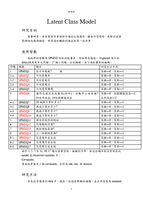
Classification log-likelihood AWE
Clusters 0.0002 0.9941 0.9899 0.9940
-48.3373 401.9457
Classification Table Probabilistic Cluster1 Cluster2 Total
Modal Cluster1 125.9795
Model2 - L?= 93.5765
2-Cluster Model
Number of cases Number of parameters (Npar)
Random Seed Best Start Seed
129 24 28856 676575
Chi-squared Statistics
Degrees of freedom (df)
答錯—0，答對—1
4-4 SPMSQ10 再減 3 等於多少?
答錯—0，答對—1
5 SPMSQ11 請告訴我你的地址。
答錯—0，答對—1
6
SPMSQ12 您母親姓什麼?
答錯—0，答對—1
7
SPMSQ13 現任總統是誰?
答錯—0，答對—1
8
SPMSQ14 上一任總統是誰?
答錯—0，答對—1
9-1 SPMSQ15 您是幾年出生的
AIC (based on L?
-53.3272
AIC3 (based on L?
-172.3272
CAIC (based on L?
-512.6449
Dissimilarity Index
0.1701
因此把它們全部歸類為只有一個 cluster 顯然不是很好。
2
林柏佐

潜类别模型（LatentClassModeling）

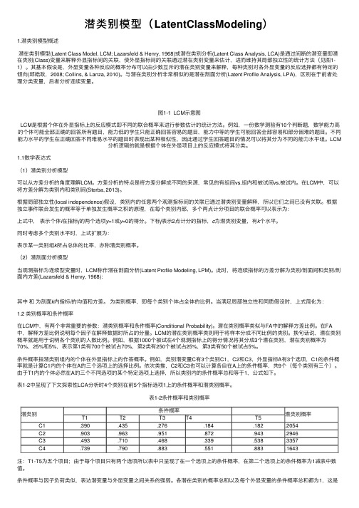
潜类别模型（LatentClassModeling）1.潜类别模型概述潜在类别模型(Latent Class Model, LCM; Lazarsfeld & Henry, 1968)或潜在类别分析(Latent Class Analysis, LCA)是通过间断的潜变量即潜在类别(Class)变量来解释外显指标间的关联，使外显指标间的关联通过潜在类别变量来估计，进⽽维持其局部独⽴性的统计⽅法（见图1-1）。

其基本假设是，外显变量各种反应的概率分布可以由少数互斥的潜在类别变量来解释，每种类别对各外显变量的反应选择都有特定的倾向(邱皓政，2008; Collins, & Lanza, 2010)。

与潜在类别分析⾮常相似的是潜在剖⾯分析(Latent Profile Analysis, LPA)，区别在于前者处理分类变量，后者分析连续变量。

图1-1 LCM⽰意图LCM是根据个体在外显指标上的反应模式即不同的联合概率来进⾏参数估计的统计⽅法。

例如，⼀份数学测验有10个判断题，数学能⼒⾼的个体可能全部正确的回答所有题⽬，能⼒低的学⽣只能正确回答容易的题⽬，能⼒中等的学⽣可能回答全部容易和部分困难的题⽬。

不同能⼒⽔平的学⽣在正确回答不同难易⽔平的题⽬时表现出某种相似性，因此通过学⽣回答题⽬的情况可以将其分为不同的能⼒⽔平组。

LCM分析逻辑的就是根据个体在外显项⽬上的反应模式将其分类。

1.1数学表达式（1）潜类别分析模型可以从⽅差分析的⾓度理解LCM。

⽅差分析的特点是将⽅差分解成不同的来源，常见的有组间vs.组内和被试间vs.被试内。

在LCM中，可以将⽅差分解为类别内和类别间(Sterba, 2013)。

根据局部独⽴性(local independence)假设，类别内的任意两个观测指标间的关联已通过潜类别变量解释，所以它们之间已没有关联。

根据独⽴事件联合发⽣的概率等于单独发⽣概率之积的原理，在每个类别内部，多个两点计分项⽬的联合概率可以表⽰为：上式中，表⽰个体i在指标j的两个选项y=1或y=0的得分。

Sociology专业英语单词

Sociology专业英语ABBehaviorism 行为主义Biculturalism 双重文化主义Bureaucracy 官僚体系Bureaucratization 科层制Bourgeoisie 资产阶级Breaching experiments 破坏性实验Because motives 原因动机Behavioral illness 行为缺陷Behavioral oganism 行为有机体Behavioral role 行为角色Bilateral descent 双边继嗣Behavioral genetics 行为遗传Born criminals 与生俱来的罪犯Baby boom 婴儿潮Class divisions 阶级分化Clinical—activist model 临床行为者模式Community control 社区控制Comparative analysis 比较分析Conspicuous consumption 炫耀性消费Crude birth rate 粗出生率Crude death rate 粗死亡率Cultural diffusion 文化传播Cultural integration 文化整合Cultural lag 文化堕距Cultural pluralism 文化多元论Conversation of gesture 姿势对话Constuctivist perspective 建构观点Collective conscience 集体意识Cultural capital 文化资本Culture of poverty 贫穷文化Action 行动Adaptation 适应Agency 能动力Alienation 异化Anomie 失范Authoritarianism 权威主义Ageism 歧视Assessment 评估Animism 泛灵论Accounting practices 项目过程的实践Affectivity affective neutrality 情感中立Achieved status 自治地位Acting crowd 行动群体Actual social identity 社会认同Affectual action 情感性活动Age norms 年龄规范Age structure 年龄结构Anticipatory socialization 预期社会化Ascription—achievement 先赋成就Autopoietic system 自我再生系统Authority bureaucratic 个体权威Authority charismatic 魅力感召性权威Authority dual 双重性权威CCapitalist 资本家Capitalism 资本主义Census 人口普查Charisma 魅力Code 符号Communism 共产主义Consummation 完成Conflict perspective 冲突论视角Conformity 遵从Correlation 相关Crowd 集群Cult 宗派Counterculture 反文化Case study 个案研究Caste system 种性制Civic privatism 公民个人主义DEEcology 生态学Ecosystem 生态系统Emigration 处境移民Endogamy 内婚制Ethnocentrism 种族中心主义Ethnomethodology 本土方法论Exogainy 外婚制Exploitation 剥削Expulsion 驱逐Ecological segregation 生态隔离Economic capitovl 经济资本Economic concentration 经济集中Egalitarion family 平权家庭Empirical method 经验性方法Estate system 等级制Ethnic group 民族群体Exchange relationship 交换关系Extended family 拓展家庭Formal organization 正式组织Formal structure 正式结构Functionalist perspective 功能主义视角Front stage 前台Functional differentiation 功能式分化Deinstitutionalization 去机制化Democracy 民主政体Demography 人口统计学Denomination 宗派Depersonalization 去个人化Deliance 越轨行为Deviant 越轨Discrimination 歧视Dogma 教义教条Dualism 二元论Dyad 对偶组二人群体Dysfunction 反功能Discourses 话语演讲Developmental questions 依赖比率Dual—earner families 拟剧论Dramaturgical perspective 双职工家庭Disaster behavior 灾后行为Deviant subculture 越轨亚文化Disciplinary society 训规社会Derian career 越轨生涯Descriptive studies 描述性研究Dependent variable 因变量Dependency theory 依赖理论Dependent chains 依赖链Democratic socialism 民主社会主义Demographic transition 人口转型Definition of the situation 情境定义FFed 时尚Fecundity 繁衍能力Fertility 生育率Field 场域理论Fieldwork 田野调查Figuration 构形Forms 形式Folkways 社会习俗Fordism 福特主义False consciousness 虚假意识Family of orientation 出身家庭Family of procreation 生育家庭Feminist theory 女性主义理论Flexible—system production 弹性生产制度GIIdeology 意识形态Incest 乱伦Impulse 冲动Industrialization 工业化Ingroups 内群体Instincts 本能Integration 整合Internalization 内化Invasion 侵入Ideal type 理想类型Illegitimate power 非法动机Impression management 印象管理Incest taboo 乱伦禁忌Independent variable 自变量In—order—to motive 企图的动机Individual culture 个人文化Infant mortality rate 婴儿死亡率Informal structure 非正式结构Institutional racism 制度化种族主义Interactionist perspective 理解/理解社会学Interest group 利益群体JJuvenile 青少年Juvenile delinquency 青少年犯罪Job enlargement 扩展工作KKinship 亲属关系NNative 本国的Negotiation 协商谈判Networks 网络Nonfunctions 非功能Normalization 正常化标准化Neonatal mortality rate 新生婴儿死亡率Nonmaterial culture 非物质遗产Nonverbal communicate 非语言沟通 Nuclear family 核心家庭Gang 帮派Gay 男同性恋Gemeinschaft 公社Gender 性别Genocide 灭绝Gerontology 老年学Governmentalities 治理性Generalized other 一般他人Generation gap 代沟Genetic structuralism 本源结构主义Group consciousness 群体意识HHomogamy 同类婚Hypothesis 假设Hysteresis 滞后Homaphobia 同性恋恐婚症Health care system 医疗保健系统Hawthorne effect 霍桑效应Hierarchical observation 阶层式监视HLV 人体免疫缺陷病毒Horizontal mobility 水平/横向流动Horizontal stratification 水平分化LLatency 潜在功能Lobbying 院外活动Labeling theory 标签理论Labor theory of value 劳动价值理论Latent functions 潜功能/隐功能Latent interests 隐形利益Legal-rational authority 法理性权威Legitimate power 合法权益Levels of functional 功能分析层次Life expectancy 预期寿命Life span 生命跨度Looking-glass self 镜中自我MMe 客我Megalopolis 大都会带Migration 移民Methodology 方法论Mob 暴民Monogamy 一夫一妻制PParticipant observation 参与观察Partition 政治区化Patriarchy 父权体系Personality 人格Politics 政体Polyandry 一夫一妻制Polygyny 一夫多妻制Post-fordism 后福特主义Predictability 可预测性Prejudice 偏见Prestige 声望Profane 世俗Proletariat 无产阶级Patriarchal family 父权家庭Patrilineal descent 父系祭祀Patrilocal residence 从夫居Pattern maintenance 模式维持/维护Peer group 同辈群体Personality system 人格体系Planned economy 计划经济Play stage 扮演期Political party 政党Population projections 人口投影法Poverty level 贫困线Postindustrial sociology 后现代社会学Postindustrial society 后工业社会Primary group 初级群体Primary socialization 初级社会化Public opinion 公众舆论Population forecast 人口预测Rumor 谣言Random sampling 随机抽样Rational-legal 法理性权威Reference group 参照群体Resource mobilization 资源动员Revolutionary movement 革命运动Rove conflict 角色冲突Role set 角色集Role performance 角色扮演Role taking 角色置换Moralize 道德论Modernization 现代化Male dominance 男性装扮Manifest function 显功能Manifest interests 显现利益Market socialism 市场社会主义Marriage gradient 婚姻倾度Mass behavior 大众行为Mass ulture 物质文化Materical social facts 物质性社会事实Matriarchal family 母家庭Matrilineal descent 母亲祭祀Matrilocal residence 从妻居Mechanical solidarity 机械团结Means-ends rational action 目标手段理性行为Migration rate 年移民率Minority group 少数名族群体Mixed economy 混合经济Multicariate analysis 多变量分析OObjective culture 客观文化Oligarchy 寡头政治Outgroup 外群体Overurbanization 过度城市化Opportunity costs 机会成本Organic solidarity 有机团结QQualitative methods 定性方法Quantitative methods 定量方法RRacism 种族主义Rationalization 理性化Reflxicity 反身性Reliability 信度Religiosity 宗教虔诚Resocialization 再社会化Role expectation 角色期待Riot 骚乱Ritual 仪式STTheism 有神话Totalitarianism 集权主义Totem 图腾Totemism 图腾崇拜Triad 三人群体Technocratic thinking 技术专家思维Theories of everyday life 日常生活理论Traditional action 传统型行为Traditional authority 传统型权威UUrbanism 城市生活方式Urbanization 城市化Utilities 效益Utopianism 乌托邦思想Urban ecologist 城市生态学家VValidity 效度Value-rational action 价值理性行动Variables 变量Verstehen 理解Vertical mobility 垂直流动Vertical stratification 垂直分层Vital statistics 动态流计Victimless crime 无受害人犯罪Voluntary association 志愿者协会WWorld association 世界体系Working class 工人阶级Succession 演替Self-segregation 自我隔离Stereotype 刻板印象Standpoint 立场Secularization 世俗化Superstructure 制约Segregation 上层建筑Self 自我Sparatism 分离主义Sexism 性别主义/歧视Stigma 污名Sect 教派Subculture 亚文化SactionSelf-control theory 自我控制Sex ratio 性别比Social deviance 社会越轨Social disorganization 社会解组Social interaction 社会互动Social control theory 社会控制理论Social mobility 社会流动Social movement 社会运动Social network 社会网络Social stratification 社会分层Social structure 社会结构Sociocultural evolution 社会文化进化论Socioeconomic status 社会经济地位Sociological imagination 社会学想象力Structural mobility 结构性流动Symbolic interactionism 符号互动论。

latent class model

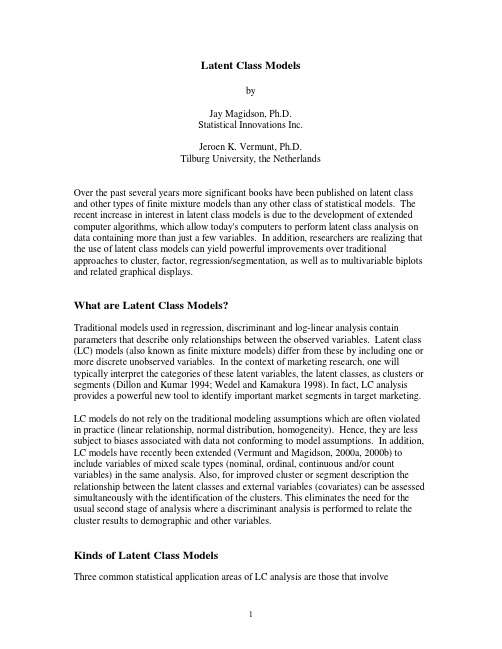
Latent Class ModelsbyJay Magidson, Ph.D.Statistical Innovations Inc.Jeroen K. Vermunt, Ph.D.Tilburg University, the NetherlandsOver the past several years more significant books have been published on latent class and other types of finite mixture models than any other class of statistical models. The recent increase in interest in latent class models is due to the development of extended computer algorithms, which allow today's computers to perform latent class analysis on data containing more than just a few variables. In addition, researchers are realizing that the use of latent class models can yield powerful improvements over traditional approaches to cluster, factor, regression/segmentation, as well as to multivariable biplots and related graphical displays.What are Latent Class Models?Traditional models used in regression, discriminant and log-linear analysis contain parameters that describe only relationships between the observed variables. Latent class (LC) models (also known as finite mixture models) differ from these by including one or more discrete unobserved variables. In the context of marketing research, one will typically interpret the categories of these latent variables, the latent classes, as clusters or segments (Dillon and Kumar 1994; Wedel and Kamakura 1998). In fact, LC analysis provides a powerful new tool to identify important market segments in target marketing. LC models do not rely on the traditional modeling assumptions which are often violated in practice (linear relationship, normal distribution, homogeneity). Hence, they are less subject to biases associated with data not conforming to model assumptions. In addition, LC models have recently been extended (Vermunt and Magidson, 2000a, 2000b) to include variables of mixed scale types (nominal, ordinal, continuous and/or count variables) in the same analysis. Also, for improved cluster or segment description the relationship between the latent classes and external variables (covariates) can be assessed simultaneously with the identification of the clusters. This eliminates the need for the usual second stage of analysis where a discriminant analysis is performed to relate the cluster results to demographic and other variables.Kinds of Latent Class ModelsThree common statistical application areas of LC analysis are those that involve1)clustering of cases,2)variable reduction and scale construction, and3)prediction.This paper introduces the three major kinds of LC models:•LC Cluster Models,•LC Factor Models,•LC Regression Models.Our illustrative examples make use of the new computer program (Vermunt and Magidson, 2000b) called Latent GOLD®.LC Cluster ModelsThe LC Cluster model:•identifies clusters which group together persons (cases) who share similar interests/values/characteristics/behavior,•includes a K-category latent variable, each category representing a cluster. Advantages over traditional types of cluster analysis include:•probability-based classification: Cases are classified into clusters based upon membership probabilities estimated directly from the model,•variables may be continuous, categorical (nominal or ordinal), or counts or any combination of these,•demographics and other covariates can be used for cluster description.Typical marketing applications include:•exploratory data analysis,•development of a behavioral based and other segmentations of customers and prospects.Traditional clustering approaches utilize unsupervised classification algorithms that group cases together that are "near" each other according to some ad hoc definition of "distance". In the last decade interest has shifted towards model-based approaches which use estimated membership probabilities to classify cases into the appropriate cluster. The most popular model-based approach is known as mixture-model clustering, where each latent class represents a hidden cluster (McLachlan and Basford, 1988). Within the marketing research field, this method is sometimes referred to as “latent discriminant analysis” (Dillon and Mulani, 1999). Today's high-speed computers make these computationally intensive methods practical.For the general finite mixture model, not only continuous variables, but also variables that are ordinal, nominal or counts, or any combination of these can be included. Also, covariates can be included for improved cluster description.As an example, we used the LC cluster model to develop a segmentation of current bank customers based upon the types of accounts they have. Separate models were developed specifying different numbers of clusters and the model selected was the one that had the lowest BIC statistic.This criteria resulted in 4 segments which were named:1)Value Seekers (15% of customers),2)Conservative Savers (35% of customers),3)Mainstreamers (40% of customers),4)Investors (10% of customers).For each customer, the model gave estimated membership probabilities for each segment based on their account mix. The resulting segments were verified to be very homogeneous and to differ substantially from each other not only with respect to their mix of accounts, but also with respect to demographics, and profitability. In addition, examination of survey data among the sample of customers for which customer satisfaction data were obtained found some important attitudinal and satisfaction differences between the segments as well. Value seekers were youngest and a high percentage were new customers. Basic savers were oldest.Investors were the most profitable customer segment by far. Although only 10% of all customers, they accounted for over 30% of the bank’s deposits. Survey data pinpointed the areas of the bank with which this segment was least satisfied and a LC regression model (see below) on follow-up data related their dissatisfaction to attrition. The primary uses of the survey data was to identify reasons for low satisfaction and to develop strategies of improving satisfaction in the manner that increased retention.This methodology of segmenting based on behavioral information available on all customers offers many advantages over the common practice of developing segments from survey data and then attempting to allocate all customers to the different clusters. Advantages of developing a segmentation based on behavioral data include:•past behavior is known to be the best predictor of future behavior,•all customers can be assigned to a segment directly, not just the sample for which survey data is available,•improved reliability over segmentations based on attitudes, demographics, purchase intent and other survey variables (when segment membership is based on survey data,a large amount of classification error is almost always present for non-surveyedcustomers) .LC Factor ModelsThe LC Factor model:•identifies factors which group together variables sharing a common source of variation,•can include several ordinal latent variables, each of which contains 2 or more levels,•is similar to maximum likelihood factor analysis in that its use may be exploratory or confirmatory and factors may be assumed to be correlated or uncorrelated(orthogonal).Advantages over traditional factor analysis are:•factors need not be rotated to be interpretable,•factor scores are obtained directly from the model without imposing additional assumptions,•variables may be continuous, categorical (nominal or ordinal), or counts or any combination of these,•extended factor models can be estimated that include covariates and correlated residuals.Typical marketing applications include:•development of composite variables from attitudinal survey items,•development of perceptual maps and other kinds of biplots which relate product and brand usage to behavioral and attitudinal measures and to demographics,•estimation of factor scores,•direct conversion from factors to segments.The conversion of ordinal factors to segments is straightforward. For example, consider a model containing 2 dichotomous factors. In this case, the LC factor model provides membership classification probabilities directly for 4 clusters (segments) based on the classification of cases as high vs. low on each factor: segment 1 = (low, low); segment 2 = (low, high); segment 3 = (high, low) and segment 4 = (high, high). Magidson and Vermunt (2000) found that LC factor models specifying uncorrelated factors often fit data better than comparable cluster models (i.e., cluster models containing the same number of parameters).Figure 1 provides a bi-plot in 2-factor space of lifestyle interests where the horizontal axis represents the probability of being high on factor 1 and the vertical axis the probability of being high on factor 2. The variable AGE was included directly in the LC Factor model as a covariate and therefore shows up in the bi-plot to assist in understanding the meaning of the factors. For example, we see that persons aged 65+ are most likely to be in the (low, high) segment, as are persons expressing an interest in sewing. As a group, their (mean) factor scores are (Factor 1, Factor 2) = (.06, .67).Since these factor scores have a distinct probabilistic interpretation, this bi-plot represents an improvement over traditional biplots and perceptual maps (see Magidson and Vermunt 2000). Individual cases can also be plotted based on their factor scores.Figure 1: Bi-plot for life-style dataThe factor model can also be used to deal with measurement and classification errors in categorical variables. It is actually equivalent to a latent trait (IRT) model without the requirement that the traits be normally distributed.LC Regression ModelsThe LC Regression model, also known as the LC Segmentation model:• is used to predict a dependent variable as a function of predictors,• includes an R-category latent variable, each category representing a homogeneous population (class, segment),• different regressions are estimated for each population (for each latent segment),• classifies cases into segments and develops regression models simultaneously.Advantages over traditional regression models include:• relaxing the traditional assumption that the same model holds for all cases (R=1)allows the development of separate regressions to be used to target each segment,• diagnostic statistics are available to determine the value for R,Factor10.00.20.40.60.8 1.0Factor21.00.80.60.40.20.0AGECAMPINGHUNTINGFISHINGWINESKNITTINGSEWINGFITNESSTENNISGOLFSKIBIKINGBOATINGGARDENTRAVEL 18-2425-3435-4445-5455-6465+camp huntfish wines knit sew fitness tennis golf ski bikeboat gardentravel•for R > 1, covariates can be included in the model to improve classification of each case into the most likely segment.Typical marketing applications include:•customer satisfaction studies: identify particular determinants of customer satisfaction that are appropriate for each customer segment,•conjoint studies: identify the mix of product attributes that appeal to different market segments,•more generally: identify segments that differ from each other with respect to some dependent variable criterion.Like traditional regression modeling, LC regression requires a computer program. As LC regression modeling is relatively new, very few programs currently exist. Our comparisons between LC regression and traditional linear regression are based on the particular forms of LC regression that are implemented in the Latent GOLD® program. For other software see Wedel and DeSarbo (1994) and Wedel and Kamakura (1998). Typical regression programs utilize ordinary least squares estimation in conjunction with a linear model. In particular, such programs are based on two restrictive assumptions about data that are often violated in practice:1)the dependent variable is continuous with prediction error normally distributed,2)the population is homogeneous - one model holds for all cases.LC regression as implemented in the Latent GOLD® program relaxes these assumptions: 1) it accommodates dependent variables that are continuous, categorical (binary, polytomous nominal or ordinal), binomial counts, or Poisson counts,2) the population needs not be homogeneous (i.e., there may be multiple populations as determined by the BIC statistic).One potential drawback for LC models is that there is no guarantee that the solution will be the maximum likelihood solution. LC computer programs typically employ the EM or Newton Raphson algorithm which may converge to a local as opposed to a global maximum. Some programs provide randomized starting values to allow users to increase the likelihood of converging to a global solution by starting the algorithm at different randomly generated starting places. An additional approach is to use Bayesian prior information in conjunction with randomized starting values which eliminates the possibility of obtaining boundary (extreme) solutions and reduces the chance of obtaining local solutions. Generally speaking, we have achieved good results using 10 randomized starting values and small Bayes constants (the default option in the Latent GOLD program).In addition to using predictors to estimate separate regression model for each class, covariates can be specified to refine class descriptions and improve classification of cases into the appropriate latent classes. In this case, LC regression analysis consists of 3 simultaneous steps:1)identify latent classes or hidden segments2)use demographic and other covariates to predict class membership, and3)classify cases into the appropriate classes/segmentsDependent variables may also include repeated/correlated observations of the kind often collected in conjoint marketing studies where persons are asked to rate different product profiles. Below is an example of a full factorial conjoint study designed to assist in the determination of the mix of product attributes for a new product.Conjoint Case StudyIn this example, 400 persons were asked to rate each of 8 different attribute combinations regarding their likelihood to purchase. Hence, there are 8 records per case; one record for each cell in this 2x2x2 conjoint design based on the following attributes:•FASHION (1 = Traditional; 2 = Modern),•QUALITY (1 = Low; 2 = High),•PRICE (1 = Lower; 2 = Higher) .The dependent variable (RATING) is the rating of purchase intent on a five-point scale. The three attributes listed above are used as predictor variables in the model and the following demographic variables are used as covariates:•SEX (1 = Male; 2 = Female),•AGE (1 = 16-24; 2 = 25-39; 3 = 40+).The goal of a traditional conjoint study of this kind is to determine the relative effects of each attribute in influencing one’s purchase decision; a goal attained by estimating regression (or logit) coefficients for these attributes. When the LC regression model is used with the same data, a more general goal is attained. First, it is determined whether the population is homogeneous or whether there exists two or more distinct populations (latent segments) which differ with respect to the relative importance placed on each of the three attributes. If multiple segments are found, separate regression models are estimated simultaneously for each. For example, for one segment, price may be found to influence the purchase decision, while a second segment may be price insensitive, but influenced by quality and modern appearance.We will treat RATING as an ordinal dependent variable and estimate several different models to determine the number of segments (latent classes). We will then show how this methodology can be used to describe the demographic differences between these segments and to classify each respondent into the segment which is most appropriate. We estimated one- to four-class models with and without covariates. Table 1 reports the obtained test results. The BIC values indicate that the three-class model is the best model (BIC is lowest for this model) and that the inclusion of covariates significantly improves the model.Table 1: Test results for regression models for conjoint dataModelLog-likelihood BIC-valueNumber ofparametersWithout covariatesOne segment-440288467Two segments-4141831915Three segments-4087831223Four segments-4080834631With covariatesTwo segments-4088828418Three segments-4036824629Four segments-4026829340The parameter estimates of the three-class model with covariates are reported in Tables 2 and 3 and 4. As can be seen from the first row of Table 2, segment 1 contains about 50% of the subjects, segment 2 contains about 25% and segment 3 contains the remaining 25%. Examination of class-specific probabilities shows that overall, segment 1 is least likely to buy (only 5% are Very Likely to buy) and segment 3 is most likely (21% are Very Likely to buy).♦Table 2: Profile outputClass 1Class 2Class 3Segment Size0.490.260.25RatingVery Unlikely0.210.100.05Not Very Likely0.430.200.12Neutral0.200.370.20Somewhat Likely0.100.210.43Very Likely0.050.110.21♦Table 3: Beta's or parameters of model for dependent variableClass 1Class 2Class 3Wald p-value Wald(=)p-value Fashion 1.97 1.140.04440.19 4.4e-95191.21 3.0e-42Quality0.040.85 2.06176.00 6.5e-38132.33 1.8e-29Price-1.04-0.99-0.94496.38 2.9e-1070.760.68The beta parameter for each predictor is a measure of the influence of that predictor on RATING. The beta effect estimates under the column labeled Class 1 suggest that segment 1 is influenced in a positive way by products for which FASHION = Modern (beta = 1.97) and in negative way by PRICE = Higher (beta = -1.04), but not by QUALITY (beta is approximately 0). We also see that segment 2 is influenced by all 3 attributes, having a preference for those product choices that are modern (beta = 1.14), high quality (beta = .85) and lower priced (beta = -0.99). Members of segment 3 preferhigh quality (beta = 2.06) and the lower (beta = -.94) product choices, but are not influenced by FASHION.Note that PRICE has more or less the same influence on all three segments. The Wald (=) statistic indicates that the differences in these beta effects across classes are not significant (the p-value = .68 which is much higher than .05, the standard level for assessing statistical significance). This means that all 3 segments exhibit price sensitivity to the same degree. This is confirmed when we estimate a model in which this effect is specified to be class-independent. The p-value for the Wald statistic for PRICE is2.9x10-107 indicating that the amount of price sensitivity is highly significant.With respect to the effect of the other two attributes we find large between-segment differences. The predictor FASHION has a strong influence on segment 1, a less strong effect on segment 2, and virtually no effect on segment 3. QUALITY has a strong effect on segment 3, a less strong effect on segment 2, and virtually no effect on segment 1. The fact that the influence of FASHION and QUALITY differs significantly between the 3 segments is confirmed by the significant p-values associated with the Wald(=) statistics for these attributes. For example, for FASHION, the p-value = 3.0x10-42.The beta parameters of the regression model can be used to name the latent segments. Segment 1 could be named the “Fashion-Oriented” segment, segment 3 the “Quality-Oriented” segment, and segment 2 is the segment that takes into account all 3 attributes in their purchase decision.♦Table 4: Gamma's: parameters of model for latent distributionClass 1Class 2Class 3Wald p-valueSexMale-0.560.71-0.1524.47 4.9e-6Female0.56-0.710.15Age16-250.84-0.59-0.2453.098.1e-1126-40-0.320.59-0.2740+-0.520.010.51The parameters of the (multinomial logit) model for the latent distribution appear in Table 4. These show that females have a higher probability of belonging to the “Fashion-oriented” segment (segment 1), while males more often belong to segment 2. The Age effects show that the youngest age group is over-represented in the “Fashion-oriented”segment, while the oldest age group is over-represented in the “Quality oriented”Segment.ConclusionsWe introduced three kinds of LC models and described applications of each that are of interest in marketing research, survey analysis and related fields. It was shown that LC analysis can be used as a replacement for traditional cluster analysis techniques, as a factor analytic tool for reducing dimensionality, and as a tool for estimating separate regression models for each segment. In particular, these models offer powerful new approaches for identifying market segments.BIOSJay Magidson is founder and president of Statistical Innovations, a Boston based consulting, training and software development firm specializing in segmentation modeling. His clients have included A.C. Nielsen, Household Finance, and National Geographic Society. He is widely published on the theory and applications of multivariate statistical methods, and was awarded a patent for a new innovative graphical approach for analysis of categorical data. He taught statistics at Tufts and Boston University, and is chair of the Statistical Modeling Week workshop series. Dr. Magidson designed the SPSS CHAID™ and GOLDMineR® programs, and is the co-developer (with Jeroen Vermunt) of Latent GOLD®.Jeroen Vermunt is Assistant Professor in the Methodology Department of the Faculty of Social and Behavioral Sciences, and Research Associate at the Work and Organization Research Center at Tilburg University in the Netherlands. He has taught a variety of courses and seminars on log-linear analysis, latent class analysis, item response models, models for non-response, and event history analysisall over the world, as well as published extensively on these subjects. Professor Vermunt is developer of the LEM program and co-developer (with Jay Magidson) of Latent GOLD® .ReferencesDillon, W.R., and Kumar, A. (1994). Latent structure and other mixture models in marketing: An integrative survey and overview. R.P. Bagozzi (ed.), Advanced methods of Marketing Research, 352-388,Cambridge: Blackwell Publishers.Dillon, W.R.. and Mulani, N. (1989) LADI: A latent discriminant model for analyzing marketing research data. Journal of Marketing Research, 26, 15-29.Magidson J., and Vermunt, J.K. (2000), Latent Class Factor and Cluster Models, Bi-plots and Related Graphical Displays. Submitted for publication.McLachlan, G.J., and Basford, K.E. (1988). Mixture models: inference and application to clustering. New York: Marcel Dekker.Vermunt, J.K. & Magidson, J. (2000a). “Latent Class Cluster Analysis”, chapter 3 in J.A. Hagenaars and A.L. McCutcheon (eds.), Advances in Latent Class Analysis. Cambridge University Press.Vermunt, J.K. & Magidson, J. (2000b). Latent GOLD 2.0 User's Guide. Belmont, MA: Statistical Innovations Inc.Wedel, M., and DeSarbo, W.S (1994). A review of recent developments in latent class regression models. R.P. Bagozzi (ed.), Advanced methods of Marketing Research, 352-388, Cambridge: Blackwell Publishers. Wedel, M., and Kamakura, W.A. (1998). Market segmentation: Concepts and methodological foundations. Boston: Kluwer Academic Publishers.。

LDA模型简介

This code base is for people interested in trying out various nonparametric Bayesian models on some simple data sets.It is implemented in MATLAB so by definition cannot be very efficient. This is because it is for people to muck around with and experiment.That said, the code is reasonably efficient. I have run it on document corpora of half a million to a million words.The code is reasonably modular and documented by README files in each section. As I get time I will release more documentation (just little technical notes) and more code.I have implemented LDA, HDP mixtures, and DP mixtures, using a varietyof sampling schemes, including Chinese restaurant process/franchise, Beta auxiliary variable method (both in HDP tech report), and a range limiting blocked Gibbs sampler (not yet published) especially for multinomials (to take advantage of vectorization in matlab).Each mixture model can use a variety of types of components. CurrentlyI only have Gaussians and multinomials, both with conjugate priors.Stay tuned.Implementations===============hdpmix Hierarchical Dirichlet process mixtures.Uses CRF, beta auxiliary variables, and range limitingblocked Gibbs (only for multinomials)lda Latent Dirichlet allocation.Uses CRP, beta auxiliary variables, and blocked Gibbs(only for multinomials).dpmix Dirichlet process mixtures.Uses CRP, beta auxiliary variables, and k-means.Pre-made Mixtures=================dpGaussianWishartDP mixture of Gaussians with Gaussian-Wishart prior.hdpMultinoimalHDP mixture of multinomials with Dirichlet prior.ldaMultinomialLDA.Tests/Demos===========testbarsDemonstrates HDP mixture and LDA trained on bars problem.testdpmixGaussianWishartDemonstrates DP mixture trained on an actual mixture of Gaussians.testpredictTests the estimated predictive likelihood given by HDP/LDA.testrandconparamTests the update scheme for the concentration parameters.=========================================================================== (C) Copyright 2004, Yee Whye Teh (ywteh -at- eecs -dot- berkeley -dot- edu)/~ywtehPermission is granted for anyone to copy, use, or modify theseprograms and accompanying documents for purposes of research oreducation, provided this copyright notice is retained, and note ismade of any changes that have been made.These programs and documents are distributed without any warranty,express or implied. As the programs were written for researchpurposes only, they have not been tested to the degree that would be advisable in any important application. All use of these programs is entirely at the user's own risk.Some simple data sets to play with.datass = gengaussian(numdim,numgroup,nummu,numdata,alpha,musigma,sigma);Generates multiple groups of data items, each group being a mixtureof Gaussians. The Gaussians are shared across groups, with eachgroup having different mixing proportions. Spherical Gaussianseach of same standard deviation.numdim dimensionality of the data.numgroup number of groups.nummu number of Gaussians.numdata number of data items per group.alpha concentration parameter for the mixing proportions of each group. musigma standard deviation of the mean of the Gaussians.sigma standard deviation of each Gaussian.datass = genbars(imsize,noiselevel,numbarpermix,numgroup,numdata);Generate bars. Each group can be seen as an image with multiplebars in it (either horizontal or vertical), with the pixel valueof each pixel being the number of data items with that value.imsize size of image.noiselevel amount of noise (noiselevel/(1+noiselvel) is actualproportion of noise).numbarpermix probabilities of generating a particular number of bars. numgroup number of groups (images).numdata number of data items drawn from each group.Dirichlet Process mixture modelling.Three implementations: chinese restaurant process, auxiliary variable method with beta variables, and k-means (always pick highest prob class).The Lexicon===========ss Sufficient statisticscc The class indexnd Number of data itemsa,b Shape and inverse scale of a gamma distribution.DP specific structures======================% numbersdp.numdata Number of data items.dp.numclass Number of classes.% data specificdp.datass(:,i) Statistics of data i.dp.datacc(1,i) Class to which data i belongs to.% class specificdp.classqq(:,k) Statistics for data and prior assigned to class k.dp.classnd(1,k) # data items in mixture j associated with class k.dp.beta(k) The beta weight associated with class k.dp.type The type of sampling scheme used: 'beta','crf','kmeans', or 'all' if all data structures are present.Parameters of the HDP=====================dp.alpha concentration parameter at bottom.dp.alphaa,alphab parameters of gamma prior on alpha.dp.qq0 A component with no data associated with it.Methods=======dp = dp_init(datass,alphaa,alphab,qq0,inittype)Constructs a representation of a DP mixture.inittype can be '1perdata', #classes (data items assigned randomly), or datacc itself.dp = dp_standardize(dp)Returns a standard representation (I use beta).dp = dp_specialize(dp,dptype)Specialize to particular sampling scheme (beta,crp,kmeans).dp = dp_iterate(dp,numiter,totiter)Runs dp for numiter iterations. If totiter is given it is usedas the total number of iterations to be run, of which this call to hdp_iterate is part of. This is just used to estimate total run time required.dp = dp_iterate(dp,numiter,totiter)Same as dp_iterate, but includes updates to the concentrationparameter.[postsample,dp] = dp_posterior(dp,numburnin,numsample,numspace);Runs dp for numburnin iterations, the collects numsample sampleswith numspace iterations in between. Returns dp at end of run,and classqq, classnd and alpha.lik = dp_predict(qq0,alldatass,postsample)Computes the predictive log likelihood of each data item inalldatass, given posterior samples. qq0 gives type of distribution.lik = dp_samplepred(qq0,alldatass,postsample,numburnin,numsample) Computes the predictive log likelihood of each data item inalldatass, given posterior samples. qq0 gives type of distribution.Uses Kass Raftery estimation.dp_crpOne iteration of Gibbs sampling in chinese restaurant process scheme.dp_betaOne iteration of Gibbs sampling with direct beta weight representation (auxiliary variables) .dp_kmeansOne iteration of k-means, assigning each data item to its highest prob class.Temporary variables===================jj index of current mixtureii index of current data item in mixture.ss Statistics of current data items.oldcc index of class of current data item (to be replaced with new sample). newcc the new sampled value for class of current data item.Unrepresented classes=====================Classes of index greater than numclass are "unrepresented classes".Beta weights can be associated with these unrepresented classes.Variables used==============dp_beta dp_crf dp_kmeansconcentration params alpha alpha alphaClass membership datacc datacc dataccclass statistics numclass numclass numclassbeta betaclassnd classnd classndclassqq classqq classqqstd->crp,kmeans: delete betacrp,kmeans->std: create beta。

latent diffusion text-to-image原理

latent diffusion text-to-image原理英文版The Principles of Latent Diffusion Text-to-ImageLatent Diffusion Text-to-Image is a cutting-edge technology that revolutionizes the field of artificial intelligence and computer vision. It combines the power of natural language processing with the capabilities of image generation, allowing users to create images from mere textual descriptions. In this article, we delve into the principles and working mechanisms behind this remarkable technology.1. Understanding the Latent SpaceLatent Diffusion Text-to-Image operates within a latent space, which is a high-dimensional vector representation of data. This space captures the underlying structure and patterns of images, allowing for efficient manipulation and generation. The latent space is learned through training a deep neural network on a large dataset of images.2. Text EncodingThe textual description provided by the user is first encoded into a fixed-size vector representation. This encoding captures the meaning and context of the text, enabling the system to understand the intent and details of the desired image. Modern natural language processing techniques, such as transformer models, are typically used for this task.3. Diffusion ProcessThe encoded text vector is then combined with a random vector from the latent space. This combination serves as the starting point for a diffusion process, which gradually transforms the random vector into an image representation. The diffusion process involves multiple steps, each refining the image based on the encoded text information.4. Image GenerationOnce the diffusion process is complete, the resulting vector is decoded into an actual image. This decoding step involves converting the high-dimensional vector back into a visualrepresentation. Modern generative models, such as convolutional neural networks (CNNs) or generative adversarial networks (GANs), are used for this purpose.5. Iterative Feedback and OptimizationThe generated image is then compared to the original textual description, and any discrepancies are fed back into the system. This feedback loop allows for iterative refinement, optimizing the generated image to better align with the user's intent.In conclusion, Latent Diffusion Text-to-Image is a powerful technology that leverages the latent space, text encoding, diffusion process, image generation, and iterative feedback to create images from textual descriptions. Its ability to bridge the gap between text and images represents a significant milestone in the field of artificial intelligence and computer vision.中文版潜在扩散文本到图像的原理潜在扩散文本到图像是一项前沿技术，彻底改变了人工智能和计算机视觉领域。

HLSM模型软件包说明书

Package‘HLSM’October12,2022Type PackageTitle Hierarchical Latent Space Network ModelVersion0.9.0Date2021-11-30Author Samrachana Adhikari,Brian Junker,Tracy Sweet,Andrew C.ThomasMaintainer Tracy Sweet<**************>Description Implements Hierarchical Latent Space Network Model(HLSM)for ensemble of net-works as described in Sweet,Thomas&Junker(2013).<DOI:10.3102/1076998612458702>. Depends R(>=4.1.0)ByteCompile TRUELicense GPL(>3)Imports MASS,coda,igraph,grDevices,graphics,methods,abind,statsLazyData yesNeedsCompilation yesRepository CRANDate/Publication2021-12-0613:00:02UTCR topics documented:HLSMcovplots (2)HLSMdiag (3)HLSMrandomEF (4)schoolsAdviceData (7)Index912HLSMcovplots HLSMcovplots Plotting functions for HLSM objectsDescriptionFunctions for plotting HLSM/LSM modelﬁts of class’HLSM’.HSLMcovplots is the most re-cent function to plot posterior distribution summaries.HLSMplotLikelihood()plots the likelihood, HLSMcovplots()summarizes posterior draws of the parameters from MCMC sample,and HLSM-plot.ﬁt.LS()is for plotting the mean latent position estimates.UsageHLSMplotLikelihood(object,burnin=0,thin=1)HLSMcovplots(fitted.model,burnin=0,thin=1)Argumentsobject object of class’HLSM’obtained as an output from LSM,HLSMrandomEF()or HLSMfixedEF()fitted.model modelﬁt from LSM(),HLSMrandomEF()or HLSMﬁxedEF()burnin numeric value to burn the chain for plotting the results from the’HLSM’object thin a numeric thinning valueValuereturns plot objects.Author(s)Sam Adhikari&Tracy SweetExamples#using advice seeking network of teachers in15schools#to fit the data#Random effect model#priors=NULLtune=NULLinitialVals=NULLniter=10random.fit=HLSMrandomEF(Y=ps.advice.mat,FullX=ps.edge.vars.mat,initialVals=initialVals,priors=priors,tune=tune,tuneIn=FALSE,dd=2,niter=niter)HLSMcovplots(random.fit)HLSMdiag3HLSMdiag Function to conduct diagnostics the MCMC chain from a random ef-fect HLSM(and HLSMﬁxedEF forﬁxed effects model)DescriptionFunction to compute and report diagnostic plots and statistics for a single or multiple HLSM objects.UsageHLSMdiag(object,burnin=0,diags=c( psrf , raftery , traceplot , autocorr ),col=1:6,lty=1)Argumentsobject object or list of objects of class’HLSM’returned by HLSMrandomEf()or HLSMfixedEF() burnin numeric value to burn the chain while extracting results from the’HLSM’object.Default is burnin=0.diags a character vector that is a subset of c( psrf , raftery , traceplot ,autocorr ).Default returns all diagnostics.If only a single chain is suppliedin object, psrf throws a warning if explicitly requested by user.col a character or integer vector specifying the colors for the traceplot and autocorrplotlty a character or integer vector specifying the linetype for the traceplot and autocorrplotValueReturns an object of class"HLSMdiag".It is a list that contains variable-level diagnostic tablesfrom either or both of the raftery diagnostic and psrf diagnostic.When returned to the console,asummary table of the diagnostics will be printed instead of the list representation of the object.call the matched call.raftery list of matrices of suggested niters,burnin,and thinning for each chain.psrf list containing psrf,a matrix of psrf estimates and upper limits for variable,andmpsrf the multivariate psrf estimate.Author(s)Christian MeyerHLSMrandomEF Function to run the MCMC sampler in random effects latent spacemodel,HLSMﬁxedEF forﬁxed effects model,or LSM for single net-work latent space model)DescriptionFunction to run the MCMC sampler to draw from the posterior distribution of intercept,slopes,and latent positions.HLSMrandomEF()ﬁts random effects model;HLSMﬁxedEF()ﬁtsﬁxed effects model;LSM()ﬁts single network model.UsageHLSMrandomEF(Y,edgeCov=NULL,receiverCov=NULL,senderCov=NULL,FullX=NULL,initialVals=NULL,priors=NULL,tune=NULL,tuneIn=TRUE,dd=2,niter)HLSMfixedEF(Y,edgeCov=NULL,receiverCov=NULL,senderCov=NULL,FullX=NULL,initialVals=NULL,priors=NULL,tune=NULL,tuneIn=TRUE,dd=2,niter)LSM(Y,edgeCov=NULL,receiverCov=NULL,senderCov=NULL,FullX=NULL,initialVals=NULL,priors=NULL,tune=NULL,tuneIn=TRUE,dd=2,estimate.intercept=FALSE,niter)getBeta(object,burnin=0,thin=1)getIntercept(object,burnin=0,thin=1)getLS(object,burnin=0,thin=1)getLikelihood(object,burnin=0,thin=1)ArgumentsY input outcome for different networks.Y can either be(i).list of sociomatrices for K different networks(Y[[i]]must be a matrix withnamed rows and columns)(ii).list of data frame with columns Sender,Receiver and Outcome for K dif-ferent networks(iii).a dataframe with columns named as follows:id to identify network,Receiver for receiver nodes,Sender for sender nodes andﬁnally,Outcome forthe edge outcome.edgeCov data frame to specify edge level covariates with(i).a column for network id named id,(ii).a column for sender node named Sender,(iii).a column for receiver nodes named Receiver,and(iv).columns for values of each edge level covariates.receiverCov a data frame to specify nodal covariates as edge receivers with(i.)a column for network id named id,(ii.)a column Node for node names,and(iii).the rest for respective node level covariates.senderCov a data frame to specify nodal covariates as edge senders with(i).a column for network id named id,(ii).a column Node for node names,and(iii).the rest for respective node level covariates.FullX list of numeric arrays of dimension n by n by p of covariates for K different networks.When FullX is provided to the function,edgeCov,receiverCov andsenderCov must be speciﬁed as NULL.initialVals an optional list of values to initialize the chain.If NULL default initialization is used,else initialVals=list(ZZ,beta,intercept,alpha).Forﬁxed effect model beta is a vector of length p and intercept is a vector oflength1.For random effect model beta is an array of dimension K by p,and interceptis a vector of length K,where p is the number of covariates and K is the numberof network.ZZ is an array of dimension NN by dd,where NN is the sum of nodes in all Knetworks.priors an optional list to specify the hyper-parameters for the prior distribution of the paramters.If priors=NULL,default value is used.Else,priors=list(MuBeta,VarBeta,MuZ,VarZ,PriorA,PriorB)MuBeta is a numeric vector of length PP+1specifying the mean of prior distri-bution for coefﬁcients and interceptVarBeta is a numeric vector for the variance of the prior distribution of coefﬁ-cients and intercept.Its length is same as that of MuBeta.MuZ is a numeric vector of length same as the dimension of the latent space,specifying the prior mean of the latent positions.VarZ is a numeric vector of length same as the dimension of the latent space,specifying diagonal of the variance covariance matrix of the prior of latent posi-tions.PriorA,PriorB is a numeric variable to indicate the rate and scale parametersfor the inverse gamma prior distribution of the hyper parameter of variance ofslope and intercepttune an optional list of tuning parameters for tuning the chain.If tune=NULL,default tuning is done.Else,tune=list(tuneBeta,tuneInt,tuneZ).tuneBeta and tuneInt have the same structure as beta and intercept ininitialVals.ZZ is a vector of length NN.tuneIn a logical to indicate whether tuning is needed in the MCMC sampling.Default is FALSE.dd dimension of latent space.estimate.interceptWhen TRUE,the intercept will be estimated.If the variance of the latent posi-tions are of interest,intercept=FALSE will allow users to obtain a unique vari-ance.The intercept can also be inputed by the user.niter number of iterations for the MCMC chain.object object of class’HLSM’returned by HLSM()or HLSMfixedEF()burnin numeric value to burn the chain while extracting results from the’HLSM’object.Default is burnin=0.thin numeric value by which the chain is to be thinned while extracting results from the’HLSM’object.Default is thin=1.DetailsThe HLSMfixedEF and HLSMrandomEF functions will not automatically assess thinning and burn-in.To ensure appropriate inference,see HLSMdiag.See also LSM forﬁtting network data from a single network.ValueReturns an object of class"HLSM".It is a list with following components:draws list of posterior draws for each parameters.acc list of acceptance rates of the parameters.call the matched call.tuneﬁnal tuning valuesAuthor(s)Sam Adhikari&Tracy SweetReferencesTracy M.Sweet,Andrew C.Thomas and Brian W.Junker(2013),"Hierarchical Network Models for Education Research:Hierarchical Latent Space Models",Journal of Educational and Behavorial Statistics.Exampleslibrary(HLSM)#Set values for the inputs of the functionpriors=NULLtune=NULLinitialVals=NULLniter=10#Fixed effect HLSM on Pitt and Spillane datafixed.fit=HLSMfixedEF(Y=ps.advice.mat,senderCov=ps.node.df,initialVals=initialVals,priors=priors,tune=tune,tuneIn=FALSE,dd=2,niter=niter)summary(fixed.fit)lsm.fit=LSM(Y=School9Network,edgeCov=School9EdgeCov,senderCov=School9NodeCov,receiverCov=School9NodeCov,niter=niter)names(lsm.fit)schoolsAdviceData HLSM:Included Data SetsDescriptionData set included with the HLSM package:network variables from Pitts and Spillane(2009). Usageps.advice.matps.advice.dfps.all.vars.matps.edge.vars.matps.edge.dfps.school.vars.matps.teacher.vars.matps.node.dfSchool9NetworkSchool9NodeCovSchool9EdgeCovFormatps.advice.mat:a list of15sociomatrices of advice seeking network,one for each school.ps.advice.df:a data frame of all ties.ps.all.vars.mat:a list of15arrays of all the covariates,one for each school.edge.vars.mat:a list of edge level covariates for15different school.ps.edge.df:a dataframe of all edge covariates.ps.school.vars.mat:a list of school level covariates for all15schools.ps.teacher.vars.mat:a list of node level covariates for all15schools.ps.node.df:a dataframe of all node covariates.ps.all.vars.mat:a single list of length15containing the covariates mentioned above.School9Network:a single adjacency matrix from School9.School9NodeCov:a dataframe with node covariatesSchool9EdgeCov:a dataframe with dyad-level covariates.Author(s)Sam AdhikariReferencesPitts,V.,&Spillane,J.(2009)."Using social network methods to study school leadership".International Journal of Research&Method in Education,32,185-207Sweet,T.M.,Thomas,A.C.,and Junker,B.W.(2012)."Hierarchical Network Models for Education Research:Hierarchical Latent Space Models".Journal of Educational and Behavorial Statistics.Index∗datasetsschoolsAdviceData,7getBeta(HLSMrandomEF),4getIntercept(HLSMrandomEF),4 getLikelihood(HLSMrandomEF),4getLS(HLSMrandomEF),4 HLSMcovplots,2HLSMdiag,3HLSMfixedEF(HLSMrandomEF),4 HLSMplot.fit.LS(HLSMcovplots),2 HLSMplot.fixed.fit(HLSMcovplots),2 HLSMplot.random.fit(HLSMcovplots),2 HLSMplotLikelihood(HLSMcovplots),2 HLSMrandomEF,4LSM(HLSMrandomEF),4print.HLSM(HLSMrandomEF),4print.summary.HLSM(HLSMrandomEF),4ps.advice.df(schoolsAdviceData),7ps.advice.mat(schoolsAdviceData),7ps.all.vars.mat(schoolsAdviceData),7ps.edge.df(schoolsAdviceData),7ps.edge.vars.mat(schoolsAdviceData),7 ps.node.df(schoolsAdviceData),7ps.school.vars.mat(schoolsAdviceData),7ps.teacher.vars.mat(schoolsAdviceData),7School9EdgeCov(schoolsAdviceData),7 School9Network(schoolsAdviceData),7 School9NodeCov(schoolsAdviceData),7 schoolsAdviceData,7summary.HLSM(HLSMrandomEF),49。

teacher latents logits 模型蒸馏

teacher latents logits 模型蒸馏模型蒸馏（model distillation）是一种用于改善深度神经网络模型性能和压缩模型大小的技术。

它通过从一个大型教师模型中抽取知识，并将其传递给一个小型学生模型来实现。

在模型蒸馏中，教师模型是一个复杂而准确的模型，通常具有大量的参数。

相比之下，学生模型则是一个简化的模型，通常具有较少的参数。

教师模型的复杂性使之能够更好地捕捉输入数据的细节和复杂性，而学生模型则可以通过从教师模型中传递的知识来学习到更多的信息，从而提高性能。

在模型蒸馏过程中，有三个重要的概念：Teacher（教师模型）、Latents（潜在变量）和Logits（输出）。

首先是教师模型（Teacher），它是一个复杂而准确的模型，通常是已经训练好的深度神经网络。

教师模型在输入数据上生成预测结果，并将这些结果作为知识传递给学生模型。

教师模型可以是一个分类模型，也可以是一个回归模型，取决于具体的任务需求。

其次是潜在变量（Latents），它是教师模型中的中间层输出。

在模型蒸馏中，教师模型的中间层输出用于传递知识给学生模型。

通常情况下，潜在变量具有较低的维度和较少的信息量，但仍然保留了原始输入数据的重要特征。

学生模型通过学习教师模型的潜在变量，可以更好地拟合输入数据。

最后是输出（Logits），它是模型在分类任务中的输出层。

在模型蒸馏中，教师模型的输出作为学生模型的目标标签。

具体来说，教师模型的输出用作学生模型损失函数的一部分，使得学生模型能够根据教师模型的预测结果来进行训练。

通过利用教师模型的输出，学生模型可以更好地拟合训练数据，并最大限度地提高性能。

模型蒸馏的优势在于它能够在性能和模型大小之间找到一个平衡点。

通过从教师模型中抽取知识，并将其传递给学生模型，学生模型可以在减少参数数量的同时保持较高的性能。

这使得学生模型更适合在资源受限的环境中部署，例如移动设备或嵌入式系统。

总结起来，teacher latents logits 模型蒸馏是一种通过从一个复杂而准确的教师模型中抽取知识，并将其传递给一个简化的学生模型来提高模型性能和压缩模型大小的技术。

1、下载文档前请自行甄别文档内容的完整性，平台不提供额外的编辑、内容补充、找答案等附加服务。
2、"仅部分预览"的文档,不可在线预览部分如存在完整性等问题,可反馈申请退款(可完整预览的文档不适用该条件!)。
3、如文档侵犯您的权益，请联系客服反馈,我们会尽快为您处理(人工客服工作时间：9:00-18:30)。

Hierarchical Latent Class Models and Statistical Foundation for TraditionalChinese MedicineNevin L.Zhang1,Shihong Yuan2,Tao Chen1,and Yi Wang1 1Hong Kong University of Science and Technology,Hong Kong,China{lzhang,csct,wangyi}@t.hk,2Beijing University of Traditional Chinese Medicine,Beijing,Chinayuanshih@Abstract.The theories of traditional Chinese medicine(TCM)origi-nated from experiences doctors had with patients in ancient times.Weask the question whether aspects of TCM theories can be reconstructedthrough modern day data analysis.We have recently analyzed a TCMdata set using a machine learning method and found that the resultingstatistical model matches the relevant TCM theory well.This is an ex-citing discovery because it shows that,contrary to common perception,there are scientiﬁc truths in TCM theories.It also suggests the possibil-ity of laying a statistical foundation for TCM through data analysis andthereby turning it into a modern science.1IntroductionIn TCM Diagnosis,patient information is collected through an overall observa-tion of symptoms and signs rather than micro-level laboratory tests.The conclu-sion of TCM diagnosis is called syndrome and the process of reaching a diagnostic conclusion from symptoms is called syndrome diﬀerentiation.There are several syndrome diﬀerentiation systems,each focusing on a diﬀerent perspective of the human body and with its own theory.The theories describe relationships be-tween syndrome factors and symptoms,as illustrated by this excerpt: Kidney yang3(Yang et al.1998)is the basis of all yang in the body.When kidney yang is in deﬁciency,it cannot warm the body and the patient feels cold,resulting in intolerance to cold,cold limbs,and cold lumbus and back.Deﬁciency of kidney yang also leads to spleen dis-orders,resulting in loose stools and indigested grain in the stool.Here syndrome factors such as kidney yang failing to warm the body and spleen disorders due to kidney yang deficiency are not directly observed.They are similar in nature to concepts such as‘intelligence’and are indirectly measured through their manifestations.Hence we call them latentvariables.In contrast,symptom variables such as‘cold limbs’and‘loose stools’are directly observed and we call them manifest variables.TCM theories involve a large number of latent and manifest variables.Abstractly speaking,they describe relationships among latent variables,and between latent variables and manifest variables.Hence they can be viewed as latent structure models speciﬁed in natural language.TCM is an important avenue for disease prevention and treatment for ethnic Chinese and is gaining popularity among others.However,it suﬀers a serious credibility problem especially in the west.One reason is the lack of rigorous randomized trials in support for the eﬃcacy of TCM herb treatments(Normile 2003).Another equally important reason,on which this paper focuses,is the lack of scientiﬁc validations for TCM theories.Researchers in China have been searching for such validations in the form of laboratory tests for more than half a century,but there has been little success.We propose and investigate a statistical approach.In the next three paragraphs,we explain the premise and the main idea of the approach.We human beings often invoke latent variables to explain regularities that we observe.Here is an experience that many might share.I(theﬁrst author) was looking at some apartment buildings nearby one night.I noticed that,for a period of time,the lighting from several apartments was changing in brightness and color at the same times and in perfect synchrony.This caught my attention and my brain immediately concluded that there must be a common cause that was responsible for changes.My brain did so without knowing what the common cause was.So,a latent variable was introduced to explain the regularity that I observed.What I tried to do next was toﬁnd the identity of the latent variable.We conjecture that,in a similar vein,latent syndrome variables in TCM were introduced to explain observed regularities about the occurrence of symptoms. Take the concept kidney yang failing to warm the body as an example. We believe that in ancient times it wasﬁrst observed that symptoms such as intolerance to cold,cold limbs,and cold lumbus and back often occur together in patients,and then,to explain the phenomenon,the latent variable kidney yang failing to warm the body was created.When explaining the phenomenon of synchronous change in lighting,I re-sorted to my knowledge about the world and concluded that the common cause must be that residents in those apartments were watching the same TV channel. Similarly,when explaining patterns about the occurrence of symptoms,ancient Chinese resorted to their understanding of the world and the human body.This explains why concepts from ancient Chinese philosophy such as yin and yang are prevalent in TCM theories.Words such as kidney and spleen also appear in TCM theories because there was primitive anatomy in ancient times.However, the functions that TCM associates with kidney and spleen are understandably diﬀerent from the functions of kidney and spleen in modern western medicine.Thus,the premise of our work is that TCM theories originated from reg-ularities ancient Chinese doctors observed in their experiences with patients. The main idea of our approach,called the latent structure approach,is to collectpatient symptom data systematically,analyze the data based on statistical prin-ciples,and thereby obtain mathematical latent structure models.If the math-ematical latent structure models match the relevant aspects of TCM theories, then we would have validated those aspects of TCM theories statistically.A case study has been conducted to test the idea.In the following,we describe the case study and report theﬁndings.2Data and Data AnalysisThe data set used in the case study involves35symptom variables,which are considered important when deciding whether a patient suﬀers from the so-called kidney deficiency syndrome,and if so,which subtype.Each variable has four possible values:none,light,medium,and severe.The data were collected from senior citizen communities,where the kidney deficiency syndrome frequently occurs.There are totally2,600records.Each record consists of values for the35 symptom variables,but there is no information about syndrome types.We refer the relevant TCM theory that explains the occurrence of the35 symptoms as the TCM kidney theory.As mentioned earlier,this is a latent structure model speciﬁed in natural language.The objective of the case study is to induce a mathematical latent structure model from the data based on statistical principles and compare it with the TCM kidney theory to see whether and how well they match.The statistical models used in the case study are called hierarchical latent class(HLC)models(Zhang2004),which were developed speciﬁcally for latent structure discovery.An HLC model is a rooted tree where each node represents a random variable.The leaf nodes represent manifest variables,while the internal nodes represent latent variables.Quantitative information includes a marginal probability distribution for the root variable and,for each of the other variables,a conditional probability distribution for the variable given its parent.The quality of an HLC model with respect to a data set is determined by the Bayesian information criterion(BIC)(Schwarz1978).According to this widely used model selection principle,a good model shouldﬁt the data well,that is,explain the regularities well,and should be as simple as possible.Toﬁnd a model with a high BIC score,one can search in the space of all possible HLC models.The current state-of-the-art is an algorithm known as HSHC(Zhang and Kocka2004).The kidney data were analyzed using the HSHC algorithm.The best model that we obtained is denoted by M.Its BIC score is-73,860and its structure is shown in Fig.1.In the model,Y0to Y34are the manifest variables that appear in the data,while X0to X13are the latent variables introduced in the process data analysis.3Latent VariablesWe now set out to compare the structure of model M with the TCM kidney theory.According to the semantics of HLC models,the left most part of modelX0(5) X1(5)X2(3)Y 0 :loosestools Y1:indigestedgraininthestoolY2:intolerancetocoldY3:coldlumbusandbackY4:coldlimbsX3(4)Y5:edemainlegsY6:facialedemaX4(4)Y7:urineleakageafterurinationY8:frequentnocturnalurinationX5(3)Y9:urinaryincontinenceY10:nocturnalenuresisY11:frequenturinationX6(3)Y12:sorelumbusandkneesY13:lumbagoX7(3)Y14:weakcubitpulseY15:weakpulseY16:lassitudeY17:prolongedillnessY18:coughwithdyspneaX8(4)Y19:lossofhairandteethX9(4)Y20:poorhearingY21:tinnitusY22:dementia Y23:weaklegsY24:poormemoryX10(5)X11(3)Y25:palpitationX12(3)Y26:HSFCVY27:tidalfeverY28:threadyandrapidpulseY29:insomnia Y30:vertigoX13(4)Y31:drytongueY32:thirstY33:yellowurineY34:oliguresisFig.1.The structure of the best model M found for kidney data.The abbreviation HSFCV stands for Hot Sensation in Five Centers with Vexation,where theﬁve centers refer to the centers of two palms,the centers of two feet,and the heart.The integer next to a latent variable is the number of possible states of the variable.M states that there is a latent variable X1that is(1)directly related to the symptoms intolerance to cold(Y2),cold lumbus and back(Y3),and cold limbs (Y4);and(2)through another latent variable X2indirectly related to loose stools (Y0)and indigested grain in the stool(Y1).On the other hand,the TCM kidney theory asserts that when kidney yang is in deﬁciency,it cannot warm the body and the patient feels cold,resulting in manifestations such as cold lumbus and back,intolerance to cold,and cold limbs.Deﬁciency of kidney yang also leads to spleen disorders,resulting in symptoms such as loose stools and indigested grain in the stool.Here,we have a good match between model M and the TCM kidney theory.The latent variable X1can be interpreted as kidney yang failing to warm the body,while X2can be interpreted as spleen disorders due to kidney yang deficiency(kyd).According to the TCM kidney theory,clinical manifestations of the kidney essence insufficiency syndrome includes premature baldness,tinnitus,deaf-ness,poor memory,trance,declination of intelligence,fatigue,weakness,and so on.Those match the symptom variables in model M that are located under X8 fairly well and hence X8can be interpreted as kidney essence insufficiency. The clinical manifestations of the kidney yin deficiency syndrome includes dry throat,tidal fever or hectic fever,ﬁdgeting,hot sensation in theﬁve cen-ters,insomnia,yellow urine,rapid and thready pulse,and so on.Those match the symptom variables under X10fairly well and hence X10can be interpreted as kidney yin deficiency.Similarly,X3can be interpreted edema due to kyd and X4can be interpreted as kidney failing to control ub,where ub stands for the urinary bladder.It is very interesting that some of the latent variables in model M correspond to syndrome factors such as kidney yang failing to warm the body,spleen disorders due to kyd,edema due to kyd,kidney failing to control ub,kidney essence deficiency,and kidney yin deficiency,as each of them is associated with only a subset of the symptom variables in the TCM kidney theory.As the latent variables were introduced by data analysis based on a statistical principle,the case study had provided statistical validation for the introduction of those syndrome factors to the TCM kidney theory and for what are asserted about their relationships with symptom variables.4Latent ClassesBy analyzing the kidney data using HLC models,we have not only obtained a latent structure,but also clustered the data in multiple ways.For example,the latent variable X1has5states.This means that the data has in one way been grouped into5clusters,with one cluster corresponding to each state of X1.We have examined the meaning of those latent classes and found that they,like the latent variables,provide statistical validations for aspects of the TCM kidney theory.The reader is referred to a longer version of the paper for the details. 5ConclusionThe TCM kidney theory was formed in ancient times,while model M was obtained through modern day data analysis.It is very interesting that they match each other well.This shows that,contrary to popular perception,there are scientiﬁc truths in TCM theories.It also suggests the possibility of laying a statistical foundation for TCM through data analysis.AcknowledgementResearch on this work was supported by Hong Kong Grants Council Grant #622105and The National Basic Research Program(aka the973Program) under project No.2003CB517106.References1.Normile,D.(2003).The new face of traditional Chinese Medicine.Science299:188-190.2.Yang,W.,F.Meng and Y.Jiang(1998).Diagnostics of Traditional Chinese Medi-cine.Academy Press,Beijing.3.Schwarz,G.Estimating the dimension of a model,Annals of Statistics,6(2):461-464,1978.4.Zhang,N.L.(2004)Hierarchical latent class models for cluster analysis,Journal ofMachine Learning Research,5(6):697–723.5.Zhang,N.L.and T.Kocka(2004).Eﬃcient Learning of Hierarchical Latent ClassModels.Proc.of the16th IEEE International Conference on Tools with Artiﬁcial Intelligence,Boca Raton,Florida.。